Self-reinforcing directionality generates truncated Lévy walks without the power-law assumption
Abstract
We introduce a persistent random walk model with finite velocity and self-reinforcing directionality, which explains how exponentially distributed runs self-organize into truncated Lévy walks observed in active intracellular transport by Chen et. al. [Nat. mat., 2015]. We derive the non-homogeneous in space and time, hyperbolic PDE for the probability density function (PDF) of particle position. This PDF exhibits a bimodal density (aggregation phenomena) in the superdiffusive regime, which is not observed in classical linear hyperbolic and Lévy walk models. We find the exact solutions for the first and second moments and criteria for the transition to superdiffusion.
Introduction. Transport in biology is crucial on multiple scales to maintain life and deviations from normal movement are hallmarks of disease and ageing Murray (2007); *murray2001mathematical; Okubo and Levin (2013). From organisms to sub-cellular molecules, their motion is usually described by persistent random walks with finite velocities (run and tumble models) Othmer et al. (1988); Hillen (2002); Tailleur and Cates (2008); Thompson et al. (2011); Mendez et al. (2010). The preference for these velocity jump models over space jump random walks arise due to the physical constraints of organisms not instantaneously jumping in space and an inertial resistance to changes in direction. In recent years, Lévy walks Zaburdaev et al. (2015) attracted attention in modelling movement patterns of living things Reynolds (2018), from sub-cellular Chen et al. (2015); Song et al. (2018); Fedotov et al. (2018); *korabel2018non to organism Raichlen et al. (2014); Ariel et al. (2015); Huda et al. (2018) scales. Until now, Lévy walks have been mostly described by coupled continuous time random walks (CTRW) Zaburdaev et al. (2015), various fractional PDEs Compte and Metzler (1997); Sokolov and Metzler (2003); Meerschaert et al. (2002); Baeumer et al. (2005); Becker-Kern et al. (2004); Uchaikin and Sibatov (2011); Magdziarz et al. (2015) and integro-differential equations Fedotov (2016); Taylor-King et al. (2016). These approaches require power-law distributed running times with divergent first and second moments as an ab initio assumption. However, in many cases this assumption is difficult to justify, leading to ongoing discussions about the origin of power-law distributed runs, the Levy walk observed in nature Jansen et al. (2012); *wosniack2017evolutionary; Reynolds (2018) and Lévy foraging hypothesis Viswanathan et al. (1999); Tejedor et al. (2012).
Experiments exhibiting Lévy-like motion cannot be modeled with pure power-law jump or running time distributions due to finite limits in physical systems Reynolds (2012). So theoretically, power-law distributions are often truncated Mantegna and Stanley (1994) or exponentially tempered Cartea and del Castillo-Negrete (2007); *sabzikar2015tempered. Specifically for active cargo transport in cells, it was discovered that the motion is composed of multiple short runs that self-organize into longer, truncated power-law distributed, uni-directional flights (truncated Lévy walks) Chen et al. (2015). Explanations for this phenomenon have been attempted in terms of self-reinforcing directionality generated by co-operative motor protein transport Chen et al. (2015). Yet, the question remains, can a persistent random walk model generate superdiffusion without power-law distributed runs through the self-organization of exponentially distributed runs?
In this Letter, we propose a new, spatially and temporally inhomogeneous persistent random walk model that generates exponentially truncated Lévy walks through self-reinforced directionality. This exponential truncation is not directly introduced but rather arises naturally from the same microscopic mechanism that generates the power-law distribution of flights. Our model differs from the traditional Lévy walk model because superdiffusion is generated by self-reinforcing directionality rather than the assumption of power-law flight distribution with infinite second moment. Simulated densities of uni-directional flight lengths from this model show excellent agreement with truncated power-law distributions observed in experiments Chen et al. (2015). It is worth noting that there are a few examples where the power-law assumption has not been used as a starting point: superdiffusion of ultracold atoms Kessler and Barkai (2012); *barkai2014area and a random walk driven by an ergodic Markov process with switching Fedotov et al. (2007).
Self-reinforcing directionality. Consider a particle moving to the right and left in 1D with constant speed and exponentially distributed running time with rate . In the standard alternating case, the particle would change directions with probability . To consider the instance when there is a probability that the particle continues in the same direction as the previous run, we introduce the transition probability matrix Cox and Miller (1965):
| (1) |
where is the conditional transition probability that the particle will continue in the positive direction given it was moving in the positive direction before. Similarly, corresponds to the particle moving in the negative direction. The standard alternating case corresponds to .
In order to model self-reinforcing directionality using the matrix , we introduce relative times, and , that the particle moves in the positive and negative direction during time . The key point is to define the probabilities in (1) as
| (2) |
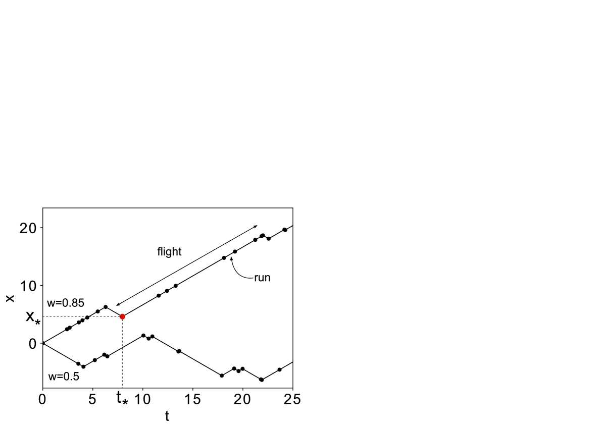
Here we introduce the persistence probability, , which parameterizes the extent that changes of direction are affected by relative times. If then the transition probabilities in both directions are the same: . If then the matrix has repetition compulsion properties: the longer a particle spends moving in the one direction, the greater the probability to maintain directionality. Figure 1 illustrates self-organization of individual runs into long uni-directional flights.
Let us show that the conditional transition probabilities (2) can be expressed in terms of particle position . Since , the relative times can be written as
| (3) |
Then substituting (3) into (2), we find that the probabilities and depend on and ,
| (4) |
Since our random walker is moving with finite speed , the relation must hold. Once again, the formula (4) shows self-reinforcing directionality since if () then the transition probability is an increasing function of particle position and the opposite for .
The equations for probability density functions (PDFs) of particles moving right () and left (), , can be written in terms of transition matrix as
| (5) |
Rearranging and taking the limit , we can write the equations for as
| (6) |
Note these equations (6) can be rewritten in terms of space and time dependent switching rates
| (7) |
These switching rates will be used to show how the exponentially truncated power-law distribution of flights arise from exponentially distributed runs. Using standard methods Mendez et al. (2010); Schnitzer (1993); Thompson et al. (2011) and equation (4), we can obtain the partial differential equations (PDEs) for total density and flux : and (See Supp. Mat.). The initial conditions are
| (8) |
where is the probability that the intial velocity is . Finally, we can find the hyperbolic PDE with a non-homogeneous in space and time advection term
| (9) |
The advection term of Eq. (9) is unconventional because it depends on the initial position . Furthermore, if the initial conditions are symmetric, (see (8)), then the average drift is zero. Clearly, (9) is a modification of the classical telegraph or Cattaneo equation Kac (1974); Schnitzer (1993); Mendez et al. (2010), with a time and space dependent advection term. In what follows, we will show that this additional term generates superdiffusion. In fact, a generalized Cattaneo equation generating superdiffusion has been formulated using the Riemann-Liouville fractional derivative Compte and Metzler (1997). The advantage of Eq. (9) over fractional PDEs is that it is far simpler and does not require integral operators in time. To the authors’ knowledge, the hyperbolic PDE (9) is the first formulation of truncated Lévy walks without integral operators Fedotov (2016). In the diffusive limit, when and such that is a constant, (9) becomes the governing advection-diffusion equation for the continuous approximation of the elephant random walk Schütz and Trimper (2004); *paraan2006exact; *da2013non; *da2020non. Note that the system of equations (6) with transition rates (4) can also be mapped to the hyperbolic model for chemotaxis Hillen and Stevens (2000); *stevens1997aggregation with an unorthodox external stimulus (see Supp. Mat.)
Moment analysis. Now, we show that the variance for the underlying random process, , exhibits superdiffusive behavior: with . The moments of random walk position, , can be found from (9) as
| (10) |
Taking the Laplace transform and solving the resulting differential equations for the first and second moments using the initial conditions, , , we can obtain and (for details see Supp. Mat.). The inverse Laplace transform gives and , where is the Kummer confluent hypergeometric function. In the long time limit (), we obtain
| (11) |
and
| (12) |
Clearly, the random walk exhibits superdiffusive behavior for . The variance, , is
| (13) |
where . Results of Monte Carlo simulations are in perfect agreement with the analytical solution of the second moment (see Supp. Mat.).
Truncated Lévy walk. In what follows, we show analytically how self-reinforcing directionality generates a truncated Lévy walk with exponentially tempered power-law distributed flights. Let us find the conditional distribution of flights given the particle changes direction at the position and time (illustrated in Fig. 1 where the particle changes velocity from to ). First, we calculate the conditional survival function, , for flights moving in the positive () and negative () direction. This function gives us the probability that the random duration of a flight, , is greater than . The rates, (7) define the conditional switching rate along the particle trajectory starting at position and time as . If we rearrange using , then
| (14) |
where . Using this, we can find the conditional survival function by . Then, we can see that the constant term in (14) produces an exponential tempering factor and the term inversely proportional to the running time, , generates a power-law with exponent . Explicitly, we can write
| (15) |
The conditional distribution of flight lengths is given by: . Each uni-directional flight is drawn from a truncated power-law distribution dependent on the position and time , where the particle changes direction. Clearly, this demonstrates the difference between our new model and the traditional Lévy walk model where the power-law distribution of flights is an a priori requirement and not dependent on and . Furthermore, our new model is able to generate superdiffusion (12) without an infinite second moment of flight times (15) through self-reinforcing directionality, unlike traditional Lévy walk models.
In addition, exponential truncation (tempering) is usually introduced by simply multiplying the power-law jump or waiting time densities by an exponential factor with an additional parameter, leading to tempered fractional calculus Cartea and del Castillo-Negrete (2007); *sabzikar2015tempered. The advantage of our model is that both exponential tempering and power-law flight distribution are generated through a single microscopic mechanism involving self-reinforced directionality and the subsequent analysis of (9) is more convenient than tempered fractional calculus. An interesting feature of our model is that despite the exponential truncation of flights, the variance (13) still exhibits superdiffusive behavior for (). Numerical simulations confirm exponentially truncated power-law conditional survival function (15) for flight times (see Supp. Mat.).
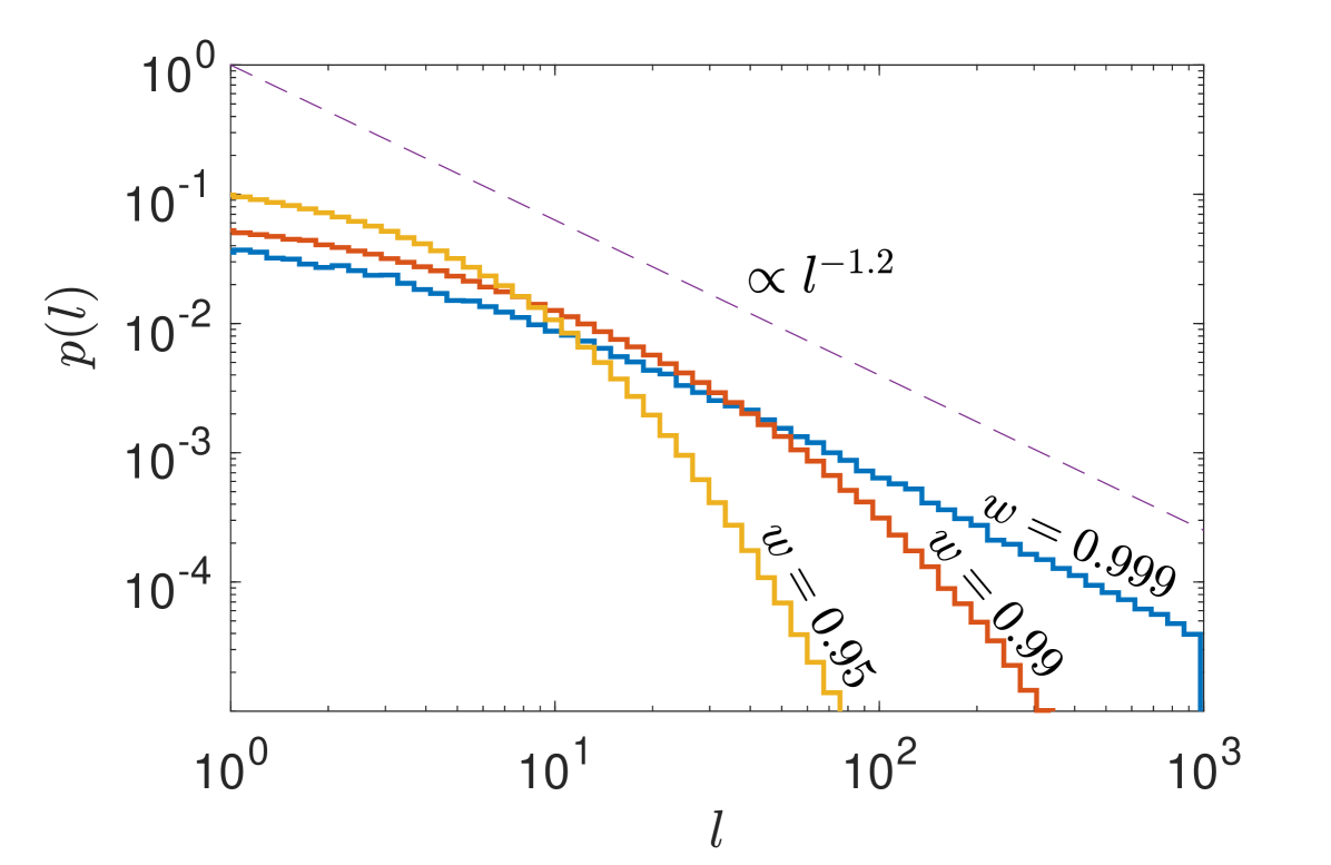
Finally, we can obtain numerically the PDF, , of flight length, , without the condition that flights begin at and . In the case of strong directionality as , should approach a pure power-law since the truncation length . Figure 2 confirms this and shows that, when , a power-law density is recovered for more than two orders of magnitude. Next, we provide evidence that the truncated power-law PDF shows excellent correspondence to published data on uni-directional endosome flights.
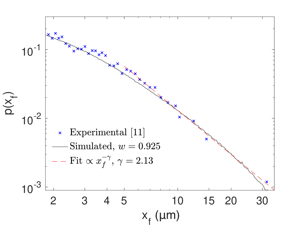
Experimental data and numerical simulations. Truncated Lévy walk behavior is observed experimentally in intracellular transport Chen et al. (2015), which arises from the self-organization of exponentially distributed runs, , into uni-directional flights, Chen et al. (2015). Here, we switch from to to avoid confusion between theoretical and experimental flights. Until now, there had been no governing PDE like (9) and an underlying persistent random walk model to describe this phenomenon. Experimentally, the authors Chen et al. (2015) report power-law tails in the flight-length density, . Figure 3 demonstrates that numerical simulations of our model are able to generate the power-law tails for flight length density and emulate the experimental data on the whole scale using reasonable parameters. Furthermore, the parameters of our new model, such as persistence probability or , rate and speed can be easily found by comparing the exact analytical formula of second moment with experimental mean squared displacements.
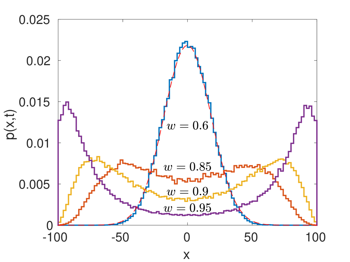
Bimodal densities and transition from diffusive to superdiffusive regime. Surprisingly, our truncated Lévy walk model in the long time limit leads to bimodal densities in the superdiffusive regime (). This phenomenon does not exist for classical superdiffusive Lévy walks. Bimodal densities (Lamperti distributions) only appear in the ballistic regime for Lévy walks with a divergent first moment for running times Uchaikin and Sibatov (2009); Klafter and Sokolov (2011); Uchaikin and Sibatov (2011); Zaburdaev et al. (2015); Froemberg et al. (2015). In the superdiffusive case, the density for Lévy walks is Gaussian in the central part with power-law tails Klafter and Sokolov (2011). This is completely different to densities for (9) (see Fig. 4). Density peaks for in (9) occur at . Figure 4 shows the emergence of a bimodal density for and , where . The density exhibits two distinct long time behaviors: it is Gaussian for () and bimodal for (). The form of the PDF also shows a non-equilibrium phase transition (see Supp. Mat.). Note that similar bimodal densities are observed in velocity random walks with interacting particles Lutscher et al. (2002); *fetecau2010investigation; *carrillo2014non; Fedotov and Korabel (2017).
For (), the variance (13) corresponds to the diffusive regime with the effective diffusion coefficient . For alternating velocity random walks, the conventional diffusion coefficient would be . As , the effective diffusion coefficient tends to infinity and this indicates the transition from the diffusive to superdiffusive regime. For the long time limit of (9) in the diffusive regime when becomes negligible, the solution is Gaussian: where . Figure 4 shows the excellent agreement between numerical simulations and the Gaussian solution for .
Self-reinforced directionality in endosome movement. Now, the question remains: what is the underlying biological mechanism explaining self-reinforced directionality in intracellular transport? To answer this question, we suggest a simple illustration of the possible origin for self-reinforced directionality. Let us consider endosomal motility, which is governed by the adaptor complexes on its membranes, the most notable being Rab GTPases Stenmark (2009). These adaptors facilitate attachment to dynein and kinesin motors Urnavicius et al. (2018) and, therefore, dictate the positioning and motility of endosomes in the cell Stenmark (2009); Gindhart and Weber (2009). To simplify this vastly complex process, consider that the endosome contains a number, , of adaptor proteins that attach to kinesin leading to transport towards the cell periphery. Similarly, is the number of adaptor proteins that attach to dynein and facilitate transport towards the cell nucleus. Then, when an endosome happens to attach to a microtubule, the simplest assumption about probabilities and in (1) would be and . However, due to the complexity of endosomal transport we can introduce a weight, , such that
From the very beginning of endocytosis until degradation, endosomes undergo a maturation process, including the association of proteins, such as Rab5 and PI(3)K Huotari and Helenius (2011). Recent work has show that effectors of Rab5 display distinct spatial densities Villaseñor et al. (2016) suggesting that and are functions of the time spent running towards, , or away, , from the cell center. So, we assume that with being some constant rate. The more an endosome moves in towards the nucleus, the more increases and vice versa. This reinforcement rule is similar to that of discrete reinforced random walks Davis (1990); Stevens and Othmer (1997). Neglecting , this formulation is exactly what leads to the repetition compulsion property in (2), since then and .
Summary. In this Letter, we developed a persistent random walk model with finite velocity that generates superdiffusion without the ab initio assumption of power-law distributed run times with infinite second moment. Our model shows that truncated power-law distributed flights can be generated from exponentially distributed runs through self-reinforcing directionality. A governing hyperbolic PDE (9) for particle probability density was derived along with exact solutions for the first and second moments. The theory is able to explain the experimentally observed self-organization of exponentially distributed runs into unidirectional flights leading to exponentially truncated Lévy walks Chen et al. (2015). We showed excellent agreement between the density of flight lengths from numerical simulations and in vivo cargo transport experiments. In the superdiffusive regime, numerical simulations of particle densities show bimodal densities (aggregation), which is a new phenomenon not seen in the classical linear hyperbolic or Lévy walk models. We believe that our methodology can be used to model migrating cancer cells Mierke et al. (2011); *mierke2013integrin; Huda et al. (2018), T-cell motility Harris et al. (2012), human foraging Raichlen et al. (2014), front propagation phenomena Méndez et al. (2004); *fedotov2015persistent, first passage time problems Redner (2001); Condamin et al. (2007); *angelani2014firstand viruses mobility inside cells Lagache and Holcman (2008); *greber2006superhighway; *dodding2011coupling.
Acknowledgements.
The authors acknowledge financial support from FAPESP/SPRINT Grant No. 15308-4 , EPSRC Grant No. EP/J019526/1 and the Wellcome Trust Grant No. 215189/Z/19/Z. We thank S. Granick for sharing experimental data; V. J. Allan, T. A. Waigh and P. Woodman for discussion.References
- Murray (2007) J. Murray, Mathematical biology: I. An introduction, vol. 17 (Springer Science & Business Media, 2007).
- Murray (2001) J. Murray, Mathematical biology II: spatial models and biomedical applications (Springer New York, 2001).
- Okubo and Levin (2013) A. Okubo and S. A. Levin, Diffusion and ecological problems: modern perspectives, vol. 14 (Springer Science & Business Media, 2013).
- Othmer et al. (1988) H. G. Othmer, S. R. Dunbar, and W. Alt, Journal of Mathematical Biology 26, 263 (1988).
- Hillen (2002) T. Hillen, Mathematical Models and Methods in Applied Sciences 12, 1007 (2002).
- Tailleur and Cates (2008) J. Tailleur and M. Cates, Physical Review Letters 100, 218103 (2008).
- Thompson et al. (2011) A. G. Thompson, J. Tailleur, M. E. Cates, and R. A. Blythe, Journal of Statistical Mechanics: Theory and Experiment 2011, P02029 (2011).
- Mendez et al. (2010) V. Mendez, S. Fedotov, and W. Horsthemke, Reaction-transport systems: mesoscopic foundations, fronts, and spatial instabilities (Springer Science & Business Media, 2010).
- Zaburdaev et al. (2015) V. Zaburdaev, S. Denisov, and J. Klafter, Reviews of Modern Physics 87, 483 (2015).
- Reynolds (2018) A. M. Reynolds, Biology Open 7, bio030106 (2018).
- Chen et al. (2015) K. Chen, B. Wang, and S. Granick, Nature Materials 14, 589 (2015).
- Song et al. (2018) M. S. Song, H. C. Moon, J.-H. Jeon, and H. Y. Park, Nature Communications 9, 1 (2018).
- Fedotov et al. (2018) S. Fedotov, N. Korabel, T. A. Waigh, D. Han, and V. J. Allan, Physical Review E 98, 042136 (2018).
- Korabel et al. (2018) N. Korabel, T. A. Waigh, S. Fedotov, and V. J. Allan, PloS One 13 (2018).
- Raichlen et al. (2014) D. A. Raichlen, B. M. Wood, A. D. Gordon, A. Z. Mabulla, F. W. Marlowe, and H. Pontzer, Proceedings of the National Academy of Sciences 111, 728 (2014).
- Ariel et al. (2015) G. Ariel, A. Rabani, S. Benisty, J. D. Partridge, R. M. Harshey, and A. Be’er, Nature Communications 6, 8396 (2015).
- Huda et al. (2018) S. Huda, B. Weigelin, K. Wolf, K. V. Tretiakov, K. Polev, G. Wilk, M. Iwasa, F. S. Emami, J. W. Narojczyk, M. Banaszak, et al., Nature communications 9, 1 (2018).
- Compte and Metzler (1997) A. Compte and R. Metzler, Journal of Physics A: Mathematical and General 30, 7277 (1997).
- Sokolov and Metzler (2003) I. M. Sokolov and R. Metzler, Physical Review E 67, 010101 (2003).
- Meerschaert et al. (2002) M. M. Meerschaert, D. A. Benson, H.-P. Scheffler, and P. Becker-Kern, Physical Review E 66, 060102 (2002).
- Baeumer et al. (2005) B. Baeumer, M. Meerschaert, and J. Mortensen, Proceedings of the American Mathematical Society 133, 2273 (2005).
- Becker-Kern et al. (2004) P. Becker-Kern, M. M. Meerschaert, H.-P. Scheffler, et al., The Annals of Probability 32, 730 (2004).
- Uchaikin and Sibatov (2011) V. Uchaikin and R. Sibatov, Journal of Physics A: Mathematical and Theoretical 44, 145501 (2011).
- Magdziarz et al. (2015) M. Magdziarz, H.-P. Scheffler, P. Straka, and P. Zebrowski, Stochastic Processes and their Applications 125, 4021 (2015).
- Fedotov (2016) S. Fedotov, Physical Review E 93, 020101 (2016).
- Taylor-King et al. (2016) J. P. Taylor-King, R. Klages, S. Fedotov, and R. A. Van Gorder, Physical Review E 94, 012104 (2016).
- Jansen et al. (2012) V. A. Jansen, A. Mashanova, and S. Petrovskii, Science 335, 918 (2012).
- Wosniack et al. (2017) M. E. Wosniack, M. C. Santos, E. P. Raposo, G. M. Viswanathan, and M. G. da Luz, PLoS Computational Biology 13, e1005774 (2017).
- Viswanathan et al. (1999) G. M. Viswanathan, S. V. Buldyrev, S. Havlin, M. Da Luz, E. Raposo, and H. E. Stanley, Nature 401, 911 (1999).
- Tejedor et al. (2012) V. Tejedor, R. Voituriez, and O. Bénichou, Physical Review Letters 108, 088103 (2012).
- Reynolds (2012) A. Reynolds, Journal of the Royal Society Interface 9, 528 (2012).
- Mantegna and Stanley (1994) R. N. Mantegna and H. E. Stanley, Physical Review Letters 73, 2946 (1994).
- Cartea and del Castillo-Negrete (2007) Á. Cartea and D. del Castillo-Negrete, Physical Review E 76, 041105 (2007).
- Sabzikar et al. (2015) F. Sabzikar, M. M. Meerschaert, and J. Chen, Journal of Computational Physics 293, 14 (2015).
- Kessler and Barkai (2012) D. A. Kessler and E. Barkai, Physical Review Letters 108, 230602 (2012).
- Barkai et al. (2014) E. Barkai, E. Aghion, and D. Kessler, Physical Review X 4, 021036 (2014).
- Fedotov et al. (2007) S. Fedotov, G. Milstein, and M. Tretyakov, Journal of Physics A: Mathematical and Theoretical 40, 5769 (2007).
- Cox and Miller (1965) D. R. Cox and H. D. Miller, The theory of stochastic processes (Chapman and Hall, 1965).
- Schnitzer (1993) M. J. Schnitzer, Physical Review E 48, 2553 (1993).
- Kac (1974) M. Kac, The Rocky Mountain Journal of Mathematics 4, 497 (1974).
- Schütz and Trimper (2004) G. M. Schütz and S. Trimper, Physical Review E 70, 045101 (2004).
- Paraan and Esguerra (2006) F. N. Paraan and J. Esguerra, Physical Review E 74, 032101 (2006).
- Da Silva et al. (2013) M. Da Silva, J. C. Cressoni, G. M. Schütz, G. Viswanathan, and S. Trimper, Physical Review E 88, 022115 (2013).
- da Silva et al. (2020) M. da Silva, E. Rocha, J. Cressoni, L. da Silva, and G. Viswanathan, Physica A: Statistical Mechanics and its Applications 538, 122793 (2020).
- Hillen and Stevens (2000) T. Hillen and A. Stevens, Nonlinear Analysis: Real World Applications 1, 409 (2000).
- Stevens and Othmer (1997) A. Stevens and H. G. Othmer, SIAM Journal on Applied Mathematics 57, 1044 (1997).
- Uchaikin and Sibatov (2009) V. Uchaikin and R. Sibatov, Journal of Experimental and Theoretical Physics 109, 537 (2009).
- Klafter and Sokolov (2011) J. Klafter and I. M. Sokolov, First steps in random walks: from tools to applications (Oxford University Press, 2011).
- Froemberg et al. (2015) D. Froemberg, M. Schmiedeberg, E. Barkai, and V. Zaburdaev, Physical Review E 91, 022131 (2015).
- Lutscher et al. (2002) F. Lutscher, A. Stevens, et al., Journal of Nonlinear Science 12, 619 (2002).
- Fetecau and Eftimie (2010) R. C. Fetecau and R. Eftimie, Journal of mathematical biology 61, 545 (2010).
- Carrillo et al. (2015) J. A. Carrillo, R. Eftimie, and F. K. Hoffmann, Kinetic & Related Models 8, 413 (2015).
- Fedotov and Korabel (2017) S. Fedotov and N. Korabel, Physical Review E 95, 030107 (2017).
- Stenmark (2009) H. Stenmark, Nat. Rev. Mol. Cell Biol. 10, 513 (2009).
- Urnavicius et al. (2018) L. Urnavicius, C. K. Lau, M. M. Elshenawy, E. Morales-Rios, C. Motz, A. Yildiz, and A. P. Carter, Nature 554, 202 (2018).
- Gindhart and Weber (2009) J. Gindhart and K. Weber (2009).
- Huotari and Helenius (2011) J. Huotari and A. Helenius, The EMBO Journal 30, 3481 (2011).
- Villaseñor et al. (2016) R. Villaseñor, Y. Kalaidzidis, and M. Zerial, Current Opinion in Cell Biology 39, 53 (2016).
- Davis (1990) B. Davis, Probability Theory and Related Fields 84, 203 (1990).
- Mierke et al. (2011) C. T. Mierke, B. Frey, M. Fellner, M. Herrmann, and B. Fabry, Journal of Cell Science 124, 369 (2011).
- Mierke (2013) C. T. Mierke, New Journal of Physics 15, 015003 (2013).
- Harris et al. (2012) T. H. Harris, E. J. Banigan, D. A. Christian, C. Konradt, E. D. T. Wojno, K. Norose, E. H. Wilson, B. John, W. Weninger, A. D. Luster, et al., Nature 486, 545 (2012).
- Méndez et al. (2004) V. Méndez, D. Campos, and S. Fedotov, Physical Review E 70, 036121 (2004).
- Fedotov et al. (2015) S. Fedotov, A. Tan, and A. Zubarev, Physical Review E 91, 042124 (2015).
- Redner (2001) S. Redner, A guide to first-passage processes (Cambridge University Press, 2001).
- Condamin et al. (2007) S. Condamin, O. Bénichou, V. Tejedor, R. Voituriez, and J. Klafter, Nature 450, 77 (2007).
- Angelani et al. (2014) L. Angelani, R. Di Leonardo, and M. Paoluzzi, The European Physical Journal E 37, 59 (2014).
- Lagache and Holcman (2008) T. Lagache and D. Holcman, SIAM Journal on Applied Mathematics 68, 1146 (2008).
- Greber and Way (2006) U. F. Greber and M. Way, Cell 124, 741 (2006).
- Dodding and Way (2011) M. P. Dodding and M. Way, The EMBO Journal 30, 3527 (2011).
Supplementary Material
.1 Derivation of the hyperbolic PDE
From (6), we can add and subtract the equations to obtain
| (S.16) |
and
| (S.17) |
Then using definitions of the total probability , the flux and conditional transition probabilities , we can write
| (S.18) |
and
| (S.19) |
Then by differentiation, (S.18) and (S.19) become,
| (S.20) |
and
| (S.21) |
Then combining (S.20) and (S.21), we obtain the hyperbolic PDE (9).
I Simulations
The simulations of our correlated random walk is as follows:
-
1.
Set initial conditions and . For initial velocity draw a uniformly distributed random number , if then and otherwise .
-
2.
Generate an exponentially distributed random time where is a uniformly distributed random number in .
-
3.
Update position and time to , respectively. For updating velocity, draw a uniformly distributed random number , then
-
(a)
If and then .
-
(b)
If and then .
-
(a)
-
4.
Repeat steps 2 and 3 until reaches the end of the simulation time .
II Moment calculations
We take the Laplace transform of (S.22) and (S.23), which gives us differential equations for , for
| (S.24) |
and
| (S.25) |
Then, solving (S.24) and (S.25) with initial conditions we obtain the analytical solutions for the first and second moments in the Letter.
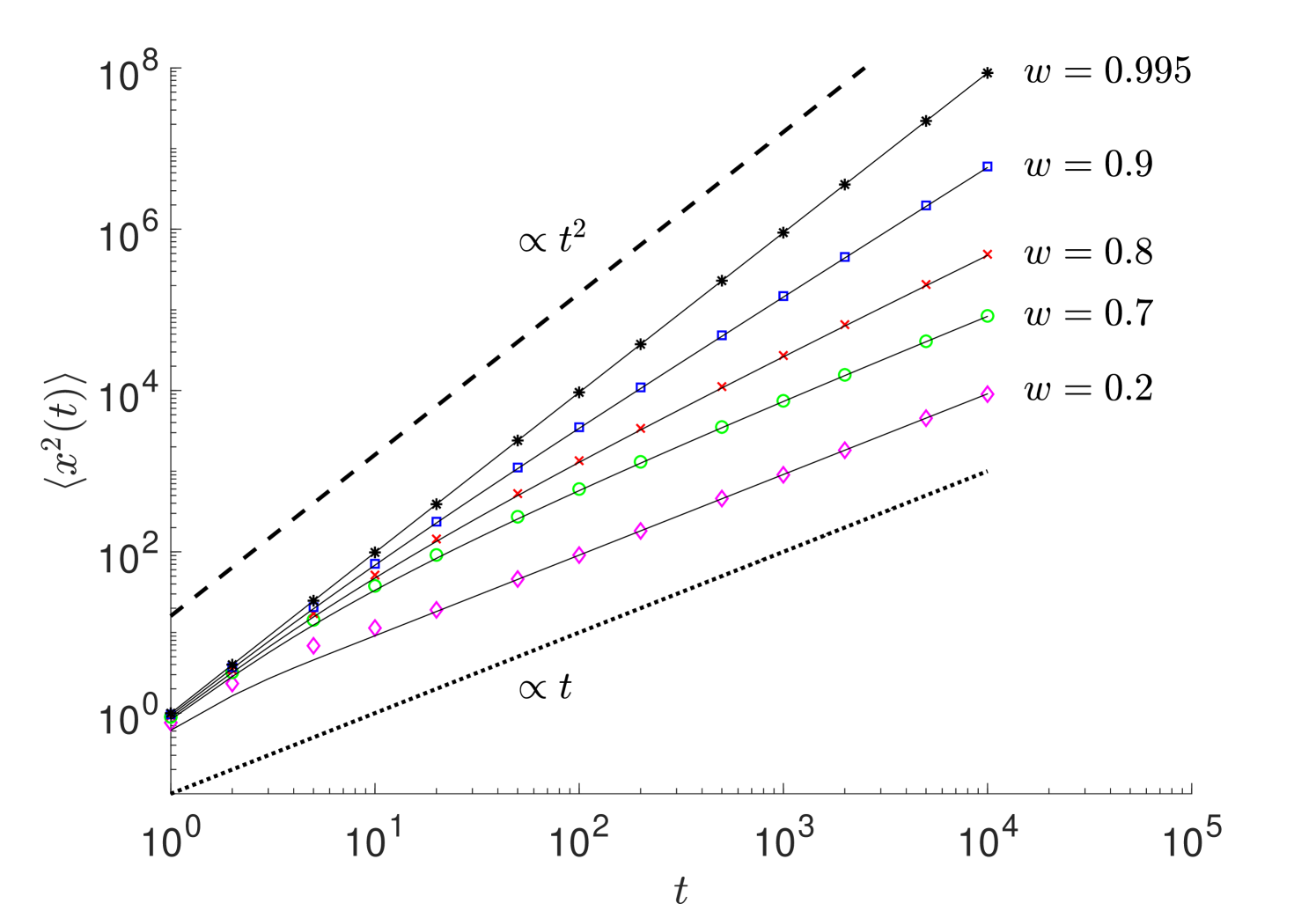
To verify our analytical results for and , we performed simulations of random walks governed by (9). From these simulations, we can measure the ensemble average mean squared displacement . Figure S5 shows excellent agreement between the analytical solutions and numerical simulations. This clearly demonstrates the emergence of superdiffusion since for (), , whereas for ().
III Link with Chemotaxis
It is interesting to note that the system of equations (6) with transition rates (4) can be mapped to the hyperbolic model for chemotaxis with an unorthodox external stimulus obeying the Hamilton-Jacobi equation for a free particle. In terms of effective turning rates, introduced in (7), that depend on the gradient of external stimulus: , with . Then the Hamilton-Jacobi equation for the external stimulus is . This provides insight into how the external stimulus, , generates superdiffusion rather than the conventional ballistic motion in chemotaxis.
IV Truncated power law flight simulations
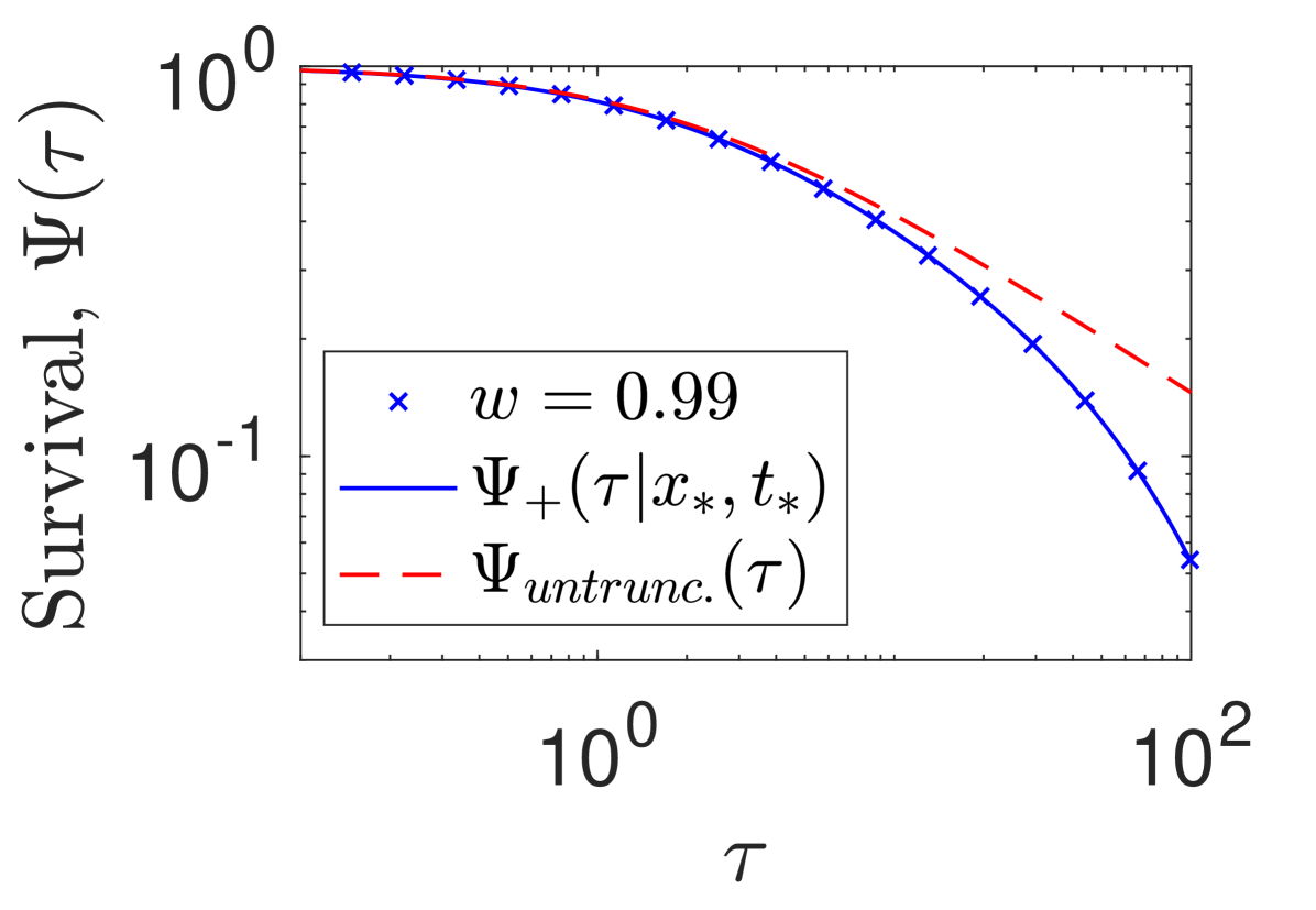
Fig. S6 shows the evidence of exponentially truncated power-law conditional survival functions and the comparison between numerical simulations and the analytical formula (20). In addition, we compare the truncated power-law survival function, from (20), to its untruncated power-law form:
| (S.26) |
V Decaying fronts at the propagation limit
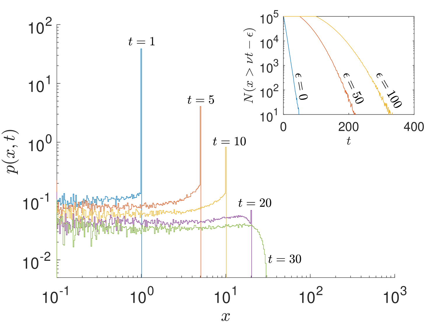
The bimodal distribution of in Fig. 4 with peaks close to the maximum position is reminiscent of the delta function horns at (‘chubchiks’) in Lévy walks [38]. They too vary similarly with the parameter , which determines the run time PDF, . For Lévy walks in the superdiffusive case (), the region near the initial position is Gaussian with the tails of the distribution having the distribution . Although our correlated random walk has similarities to Lévy walks, the major difference in the asymptotic density is the continuous distribution of the bimodal peaks at positions instead of the chubchiks seen in Lévy walks at .
In essence, the chubchiks of Lévy walks appear due to the group of particles that have been moving at the propagation velocity for the entire time and thus form a propagating front. Intriguingly, these fronts also appear for our correlated random walk but at very short times shown by Fig. S7. However, these propagating fronts decay exponentially with time whereas for Lévy walks they decay as (). By , the propagating front has completely ‘evaporated’ and the tail is now exponential with no trace of the original front. This phenomenon is intuitive since particles performing our correlated random walk take exponentially distributed runs, abeit in a persistent manner, but Lévy walks take power-law distributed runs. Exponential decay of the fronts can be seen in the inset of Fig. S7 where the number of particles with position is plotted as a function of time .
The evaporation of the propagating front demonstrates a non-equilibrium phase transition since the PDF shows chubchiks for short times that decay into exponential tails for long times. This shows the non-stationary nature of the random walk generated by (9) and the transition from Lévy walk like behavior at short times to a completely novel distribution for long times.