Self-similarity of temporal interaction networks arises from
hyperbolic geometry with time-varying curvature
Abstract
The self-similarity of complex systems has been studied intensely across different domains [1, 2, 3, 4, 5, 6] due to its potential applications in system modeling, complexity analysis, etc., as well as for deep theoretical interest. Existing studies rely on scale transformations conceptualized over either a definite geometric structure of the system [6, 7, 8, 9] (very often realized as length-scale transformations) or purely temporal scale transformations [10, 3]. However, many physical and social systems are observed as temporal interactions among agents without any definitive geometry. Yet, one can imagine the existence of an underlying notion of distance as the interactions are mostly localized. Analysing only the time-scale transformations over such systems would uncover only a limited aspect of the complexity. In this work, we propose a novel technique of scale transformation that dissects temporal interaction networks under spatio-temporal scales, namely, flow scales. Upon experimenting with multiple social and biological interaction networks, we find that many of them possess a finite fractal dimension under flow-scale transformation. Finally, we relate the emergence of flow-scale self-similarity to the latent geometry of such networks. We observe strong evidence that justifies the assumption of an underlying, variable-curvature hyperbolic geometry that induces self-similarity of temporal interaction networks. Our work bears implications for modeling temporal interaction networks at different scales and uncovering their latent geometric structures.
I Introduction
Scale invariance is defined as the characteristic of a dynamical system when its topological/dynamic properties remain the same at different scales [11, 12, 13, 14, 15] such as length, time, and size. Precisely, if one represents such properties of the system as a function of (spatial/temporal) scale , then for a scale-invariant system, we have for some arbitrary constant and being scale-independent component [16]. In the case of discrete scale transformations, scale invariance is also identified as self-similarity, i.e., the system under consideration consists of repeating patterns under different length-scales. Certain real-world complex networks have been shown to exhibit self-similarity [6, 17, 18, 19, 20, 21]. A popular approach to testing this property of networks is the box-counting method [6, 7, 22, 23]. Conceptually, the size of the box parameterizes the length-scale transformation of the networks; for a self-similar network, the number of boxes needed to cover the network is inversely proportional to a constant power of the size of the box.
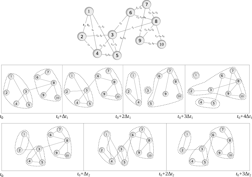
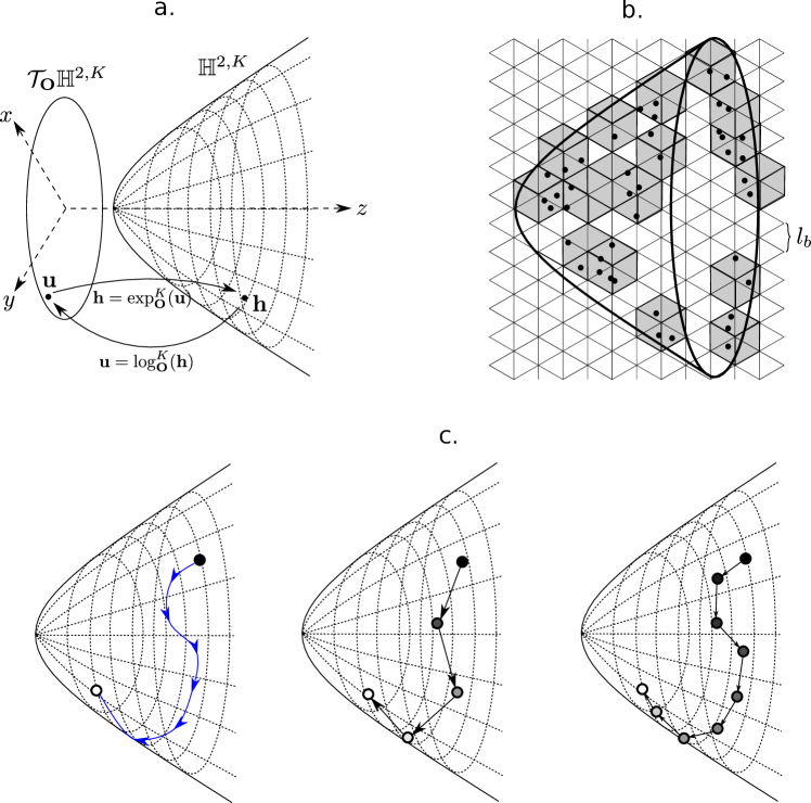
However, these existing methods of scale transformations become limited once we go beyond the static network regime. For a dynamically evolving network, one should consider the time-scale alongside the length-scale (i.e., the temporal evolution of topological properties of the network under different time-scales). The problem is even more challenging in the case of temporal interaction networks (e.g., protein-protein interactions, social interactions over online or physical platforms, etc.). Unlike networks like WWW or routing networks, where there are temporally finite connections between nodes (and, as a result, a tangible geometry over which one can define the idea of length-scale), in the case of interaction networks, the connection between any two nodes is a momentary event. As shown in Figure 1, the geometry of the network quickly changes depending upon the choice of time-scale. In essence, the length- and time-scales become inseparable when discussing the scale transformation and scale invariance of such networks.
Here we propose a novel spatio-temporal box-counting method that analyzes temporal interaction networks under simultaneous length- and time-scale transformations, which we define as flow-scale transformation. We find that interaction networks can be either scale-invariant, fractal, or non-fractal under such a transformation. We relate this to an underlying hyperbolic geometry; erratically moving random particles over a hyperbolic surface is a fractal object under flow-scale transformation. Furthermore, we empirically observe that a scale-invariant or self-similar point-particle motion can only be observed when the negative curvature of the underlying hyperboloid increases exponentially over time. This expands upon the previous works [24, 25, 26, 27] of embedding static hierarchical network structures into constant curvature hyperbolic geometry, which fails to exhibit self-similar behavior when the temporal regime is taken into account.
| Name | Type of interaction | Duration | ||
|---|---|---|---|---|
| ia-email [28] | Email interactions | 56931 | 762462 | 720 days |
| reddit-hyperlink [29] | Interaction among subreddits via users posting hyperlinks | 33870 | 299016 | 720 days |
| DPPIN-Babu [30] | Protein-protein interaction | 4924 | 111466 | 36 units |
| ca-cit [31] | Arxiv High Energy Physics paper citation network | 16763 | 2268171 | 2160 days |
| superuser [32] | Comments, questions, and answers on Super User | 188992 | 1309161 | 2160 days |
| wiki-talk [32] | Talkpage interactions among Wikipedia editors | 45443 | 468798 | 990 days |
II Results
II.1 Discrete scale transformation of temporal networks
For static networks, box-covering provides the most popular approach to test discrete scale invariance. Given a network , a box-cover of size can be defined as , such that, the minimum distance between any two nodes in is at most . The fractal dimension of the network is defined as,
| (1) |
where is the number of nodes in the network, ; is the number of boxes of size required to cover the network, , and . A network is fractal if is finite. Furthermore, if remains constant as varies, then the network is length-scale invariant or self-similar. The term typically defines the average number of nodes in each box, or its mass; for a scale-invariant network, the mass of a box follows a power-law variation with its size [6, 7].
Temporal interaction networks naturally extend the spatial scale transformation to the temporal domain, yet it remains unexplored in the literature. A temporal interaction network can be formalized as , where each edge is a triplet for , and is the timestamp of the corresponding interaction. A popular approach of temporal graph learning is to represent as a sequence of static snapshots by sampling interactions with a given time window ; each is constructed such that for any , if , are added to and the edge is added to . As shown in Figure 1, the size of the sampling window dictates the granularity of approximation: the smaller the window, the closer the snapshots are to the actual interaction network. Therefore, the sampling time window size provides a temporal analogue of the box size . Putting them together, we define the modified box counting for a temporal interaction network . For a given box size and a sampling time size , the box-cover is defined as:
| (2) |
For brevity, we will denote as henceforth. Furthermore, we define the total number of vertices in the span for time-window size as . In Figure 1, we show a working example. For the given network, , whereas .
Therefore, if we define the volume of the spatio-temporal boxes as , then one can redefine Equation 1 in case of temporal networks as,
| (3) |
Similar to its static counterpart, a temporal network is scale-invariant if is constant for all scale sizes , and a fractal for a finite limiting value of . For a temporal scale size of , the term again defines the number of nodes within scale volume . A detailed description of flow-scale transformation is presented in Methods.
II.2 Scale transformation properties of real interaction networks
Equipped with spatio-temporal scale transformation defined in Equation 2, we analyze six different temporal interaction networks arising from various real-world interactions – Enron email interactions [28] (ia-email), Reddit hyperlink interactions [29] (reddit-hyperlink), Arxiv high-energy physics papers citations [31] (ca-cit), protein-protein interactions [30] (DPPIN-Babu), Wikipedia talkpage interactions [32] (wiki-talk) and user interactions via posts and comments on the Superuser forum [32] (superuser) (see Table 1 for various statistics of these datasets). The choice of networks encompasses a wide variety of interactions: from user interactions over social platforms to protein-protein interactions. Furthermore, the list includes very slow-growing (e.g., citation networks) to very fast-growing (e.g., Reddit or Superuser) networks. We need to set different sizes for the time window in different networks to cope with this variation of interaction density.
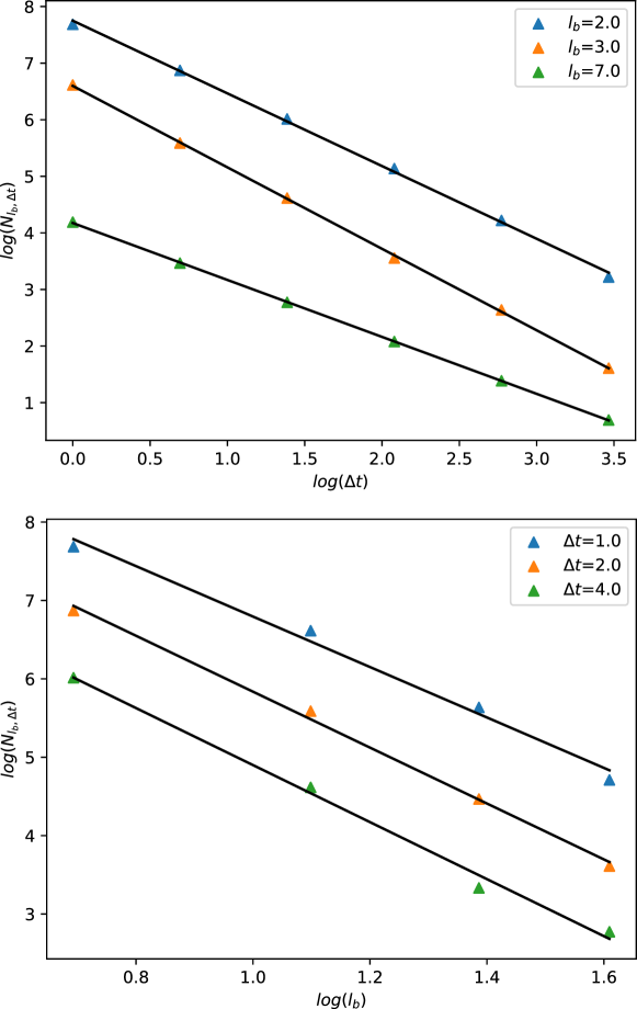
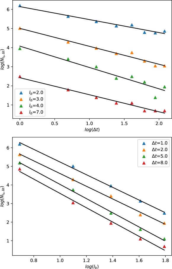
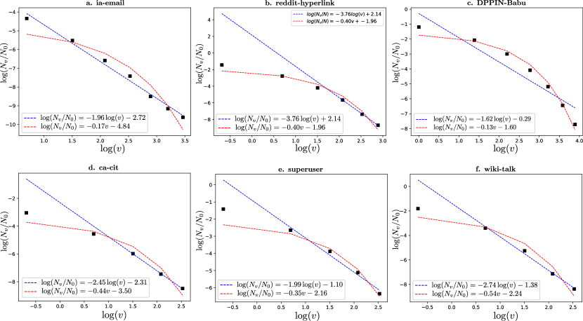
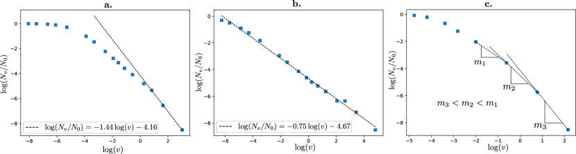
In Figure 2, we summarize the scale transformation properties of these networks. Equation 3 indicates that there can be three possible patterns for a network to exhibit: i) a linear variation of vs denoting scale-invariance, ii) a linear variation of with for larger values of , denoting a finite fractal dimension but not scale-invariance, and iii) no linear relationship between and , denoting a non-fractal network. The box-counting estimation of fractality and scale invariance is inherently statistical. Since the networks in consideration are finite, a small degree of noise can skew the presence (or absence) of linear relationships among observed samples. To deal with this, we fit two regression curves, one assuming (i.e., a finite fractal dimension) and another assuming (i.e., as ). As Figure 2 suggests, all the networks except DPPIN-Babu and superuser have a finite fractal dimension in the limiting case. We can calculate the value of the corresponding fractal dimensions from the slope of the regression lines – for ia-email, for reddit-hyperlink, for ca-cit, and for wiki-talk. Among these fractal networks, only ia-email shows scale-invariant characteristics under flow-scale transformations.
We further experiment on the scaling properties of some of these networks under purely spatial or temporal scale transformations (see Supplementary, Figures S1 to S4). As we can observe, a finite fractal dimension under flow-scale transformation necessitates scale-invariance under both length- and time-scale transformations. Failure in either of these conditions would lead to non-fractal behaviour (like DPPIN-Babu).
II.3 Point-particle motion on hyperbolic surface
One can intuitively identify the proposed flow-scale boxes as a potential volume of influence of a cluster of nodes over both space as well as time. As we go from smaller to larger time-scales as well length-scales, the chances of a node interacting with other nodes increase. This eludes one to draw an analogy between a temporal interaction network and a system of point particles moving randomly in space; the chance of two particles interacting with each other increases as they come closer in space. Such an analogy naturally presumes a latent geometry of the point-particle system. It has been shown previously that an assumption of underlying non-Euclidean space explains the emergence of self-similarity in complex networks [19, 33]. Following the precedence of linking hyperbolic geometry to the evolution of complex networks [34, 35], we investigate the spatial and temporal scale transformation properties of discrete objects on hyperbolic space to seek parallels with the temporal information networks. Please see Methods for constructing necessary structures of hyperbolic geometry in terms of the Lorentzian model.
By definition of hyperbolic geometry, points closer to the origin have a shorter geodesic distance compared to points further away (Figure 3 b.). This provides us with a natural analogy to complex networks. For example, a hub, which is reachable from other nodes with a shorter path, can be represented as a point near the origin (and peripheral nodes can be mapped further away). Furthermore, the Lorentzian model equips us with the property that one can define operations on the Euclidean tangent space with minimal complexity and map them back to the hyperbolic space using the exponential map. With this, we proceed to define the point-particle motion over .
We define the process over the timespan . A point-particle is characterized by its position and velocity vectors on the tangent space at the origin, . At any timestamp , a point-particle is initialized at position randomly over . The ‘true’ or latent trajectory of the particle is governed by a parametric estimation of the velocity given by
| (4) |
where are random parameters that characterize . This latent trajectory is intrinsic to the particle-system and, therefore, can not be observed directly. Instead, the system is realized in discrete timestamps , as shown in Figure 3 c. The position of a particle over at time can be calculated as
| (5) |
and then mapped to using the exponential map. With equally spaced timestamps ’s and , the sequence of particle positions approach the true trajectory as . This serves the purpose of the time-scale transformation similar to Equation 2. Since in the hyperboloid model, is immersed in , the natural choice of defining the length-scale transformation is via covering the particle system with -dimensional grids of size , as shown in Figure 3 b. With these two definitions, we can directly define the fractal dimension of this particle system as the same as in Equation 3.
II.4 Scale-invariance and time-varying curvature
The point-particle motion described in the previous section can be majorly characterized by two parameters: the curvature of the space and the choice of the distribution from which the initial particle positions are sampled.
We experiment with three different scenarios in terms of curvature. Our procedures defined in the previous section already demonstrate the constant negative curvature scenario: the particle position at any time is found via mapping to using the exponential map (Equation 11). An analogous phenomenon over a zero curvature (i.e., Euclidean) space can be achieved if and are defined over instead of and scale transformations are applied over them directly instead of applying an exponential map. Finally, we experiment with a space with negative curvature varying with time. This can be achieved using the following definition of the exponential map:
| (6) |
Here, the origin shifts with time since it is defined explicitly using the curvature of the space.
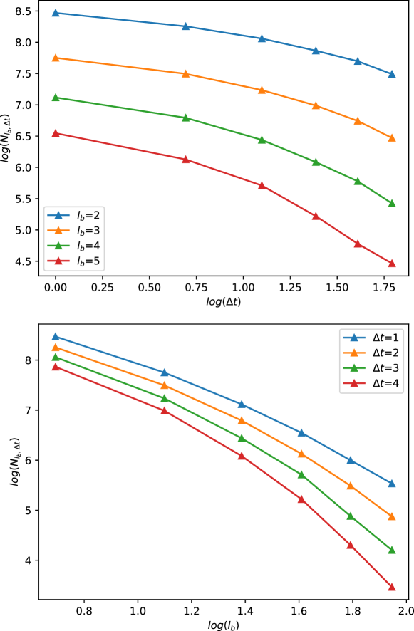
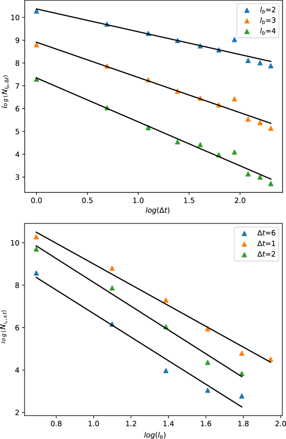
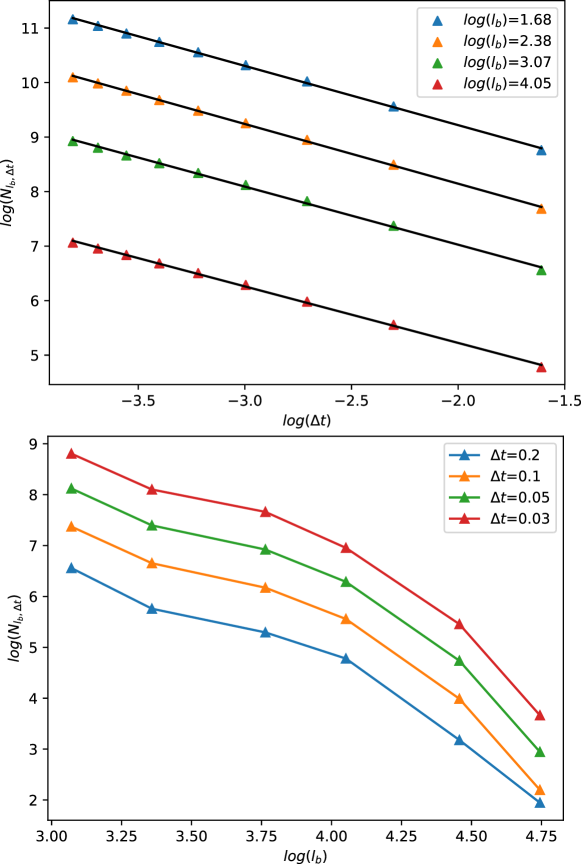
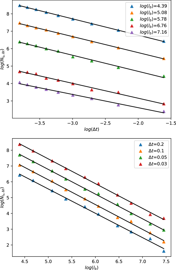
Additionally, we experiment with the particle positions initially sampled from a Gaussian vs a uniform distribution, both centred at the origin of . We find that the three distinctive patterns of scale transformation that we observed in the case of the real networks emerge with specific choices of curvature and distributions in the point-particle motion as well, as shown in Figure 4. When the particle positions are sampled uniformly over a constant curvature space, we observe that the fractal dimension, albeit non-constant, converges to a finite value as . We conclude that a constant negative curvature space almost always guarantees a finite fractal dimension but not a scale-invariant one (Figure 4 a. shows the variation with and ). Scale-invariance exclusively arises when we move to space with time-varying negative curvature, specifically, for some positive constants and ; in the example shown in Figure 4 b., , , . Finally, a particle set initialized from a Gaussian over the flat Euclidean space fails to exhibit a finite fractal dimension (Figure 4 c. with and a zero mean unit standard deviation Gaussian).
III Discussion
We developed a method for spatio-temporal scale transformations over temporal interaction networks lacking predefined geometry. Our described method relied upon a coarsening of time-scale to build static snapshots of the interaction stream that can be treated as networks induced by simultaneous interactions. Our analysis of multiple real-world interaction networks suggested the emergence of finite fractal dimensions under our proposed notion of flow-scale transformations. In an attempt to link such invariance properties to a latent geometry of the networks, we simulated point-particle trajectories over hyperbolic space. These point-particle systems served as a parallel to temporal interaction networks, similar to the previous notion of random geometric graphs in which the probability of forming an edge between any two nodes embedded in a geometry is proportional to the distance between these nodes. Emulating the time-scale coarsening and grid-covering over the ambient space of these particle systems revealed that a scale-invariant system is possible only when the underlying hyperbolic space has a time-varying curvature (to be specific, an exponentially increasing value of negative curvature). Flat geometries fail to show a bounded fractal dimension.
One major challenge in discussing the scaling properties of real-world networks is that these networks are finite-size, and scale-invariant properties are often hidden under noises [36, 37]. Our work also exhibits the same limitations – most of the temporal interaction networks we considered are of moderate size, and their scaling characteristics are skewed when the flow-scale boxes are small. However, the strong parallel between the scaling properties of the real-world networks and those of the point-particle trajectories in latent geometric spaces materializes the phenomena beyond domain-dependent artefacts. Our findings are particularly useful towards modeling social/biological networks. Linking the latent space model with the scaling properties of temporal interaction networks, our findings can broaden the understanding of network embedding methods — a core problem in the predictive modeling of interaction networks. Finally, our work may facilitate the applications of more general understandings of critical processes in statistical physics [38, 39, 40, 41] that depict scale-invariance to the specific problems of network science.
IV Materials and Methods
IV.1 Defining flow-scale boxes
The definition of flow-scale boxes requires simultaneous scale transformation over space as well as time. To define the time-scale transformation, we use successive coarsening of the temporal measure that instantiates the interaction timestamps in the following manner.
Let a temporal interaction network be defined as a chronologically ordered sequence of time-stamped interactions , where and are the start and end times of the interactions, respectively, and and are any two nodes interacting at time . The discrete nature of these timestamps presumes that the observation was done at a certain degree of coarsening, i.e., they are measured to the nearest integer value on a specific unit of time like seconds, hours, or days. To illustrate further with an example, if the timestamps are reported in integer seconds, and if an interaction actually occurred at time seconds, then the timestamp that will be associated with the said interaction will be seconds. Therefore, it will be treated as contemporary with another interaction happening at a time of seconds. In this example, the chosen scale of time is second. We extend this to any arbitrary time-scale to renormalize the network. Given a time-scale , the renormalized interaction network can be defined as:
| (7) |
for any such that . Such a time-scale renormalization treats any interaction happening within the window as contemporary, thereby segmenting into static snapshots. Each of these snapshots can be considered a static network constructed by nodes interacting with each other simultaneously (under the time-scale renormalization). The -th snapshot is then defined as with and being the set of nodes and edges, respectively such that, for any , there exists at least one interaction .
These snapshots now bear a geometric structure (i.e., the distance between two nodes can be defined based on the path length) conditioned upon the concept of simultaneity introduced by the coarsening of the time-scale. This allows us to apply box-counting to initiate length-scale renormalization.
Next, we apply box-covering to perform length-scale renormalization on the snapshots. We use the Maximum Excluded Mass Burning (MEMB) algorithm [42] to count the number of boxes of a given size needed to cover a given snapshot . MEMB defines boxes with their radius instead of diameter. A box of radius is a connected subgraph with a root node of arbitrary choice such that any node in the subgraph is at most distance away from the root node. The number of boxes to cover the interaction network is then,
| (8) |
where is the number of flow-scale boxes of time-scale and length-scale needed to cover the temporal interaction network . Details of the choices of parameter sizes for different datasets are described in Supplementary, Table S1.
IV.2 Lorentzian model of hyperbolic geometry
We start with the -dimensional, Lorentzian Hyperboloid model of the hyperbolic space, denoted by of constant negative curvature , embedded in an -dimensional space (i.e., ). For any two points , we have the Minkowski inner product:
| (9) |
For any , we have . The tangent space to at point is defined as,
| (10) |
For any point , the Minkowski norm is defined by . The origin of is defined as where and for all . One can define a bijective map between and , also called the exponential map, as,
| (11) |
for and . The inverse of the exponential map is called the logarithmic map and is defined as,
| (12) |
where is the distance (length of the geodesic curve) between and .
Data and Source Code Availability
The datasets used in this paper are publicly available at https://snap.stanford.edu and https://networkrepository.com. The source codes is available at https://github.com/Subha0009/Temporal-network-self-similarity.
Supplementary Information
The supplementary contains additional information related to network datasets, experimental setup, and results.
Acknowledgement
T.C. would like to acknowledge the support of the Ramanujan Fellowship (SB/S2/RJN-073/2017), funded by the Science and Engineering Research Board (SERB), India.
References
- Paxson and Varanasi [2013] A. T. Paxson and K. K. Varanasi, Self-similarity of contact line depinning from textured surfaces, Nature Communications 4, 1492 (2013).
- Rydelek and Sacks [1989] P. A. Rydelek and I. S. Sacks, Testing the completeness of earthquake catalogues and the hypothesis of self-similarity, Nature 337, 251 (1989).
- Hsü and Hsü [1991] K. J. Hsü and A. Hsü, Self-similarity of the” 1/f noise” called music., Proceedings of the National Academy of Sciences 88, 3507 (1991).
- Simini et al. [2010] F. Simini, T. Anfodillo, M. Carrer, J. R. Banavar, and A. Maritan, Self-similarity and scaling in forest communities, Proceedings of the National Academy of Sciences 107, 7658 (2010).
- Teo and Zhang [1991] B. K. Teo and H. Zhang, Clusters of clusters: self-organization and self-similarity in the intermediate stages of cluster growth of au-ag supraclusters., Proceedings of the National Academy of Sciences 88, 5067 (1991).
- Song et al. [2005] C. Song, S. Havlin, and H. A. Makse, Self-similarity of complex networks, Nature 433, 392 (2005).
- Gallos et al. [2007a] L. K. Gallos, C. Song, and H. A. Makse, A review of fractality and self-similarity in complex networks, Physica A: Statistical Mechanics and its Applications 386, 686 (2007a).
- Zheng et al. [2020] M. Zheng, A. Allard, P. Hagmann, Y. Alemán-Gómez, and M. Á. Serrano, Geometric renormalization unravels self-similarity of the multiscale human connectome, Proceedings of the National Academy of Sciences 117, 20244 (2020).
- Gallos et al. [2007b] L. K. Gallos, C. Song, and H. A. Makse, A review of fractality and self-similarity in complex networks, Physica A: Statistical Mechanics and its Applications 386, 686 (2007b).
- Proekt et al. [2012] A. Proekt, J. R. Banavar, A. Maritan, and D. W. Pfaff, Scale invariance in the dynamics of spontaneous behavior, Proceedings of the National Academy of Sciences 109, 10564 (2012).
- Krug [1997] J. Krug, Origins of scale invariance in growth processes, Advances in Physics 46, 139 (1997).
- Sornette [1998a] D. Sornette, Discrete-scale invariance and complex dimensions, Physics reports 297, 239 (1998a).
- Cohen and Havlin [2004] R. Cohen and S. Havlin, Fractal dimensions of percolating networks, Physica A: Statistical Mechanics and its Applications 336, 6 (2004).
- Stanley et al. [2000] H. E. Stanley, L. Amaral, P. Gopikrishnan, P. C. Ivanov, T. Keitt, and V. Plerou, Scale invariance and universality: organizing principles in complex systems, Physica A: Statistical Mechanics and its Applications 281, 60 (2000).
- Guimera et al. [2003] R. Guimera, L. Danon, A. Diaz-Guilera, F. Giralt, and A. Arenas, Self-similar community structure in a network of human interactions, Physical review E 68, 065103 (2003).
- Sornette [1998b] D. Sornette, Discrete-scale invariance and complex dimensions, Physics reports 297, 239 (1998b).
- Song et al. [2006] C. Song, S. Havlin, and H. A. Makse, Origins of fractality in the growth of complex networks, Nature physics 2, 275 (2006).
- Goh et al. [2006] K.-I. Goh, G. Salvi, B. Kahng, and D. Kim, Skeleton and fractal scaling in complex networks, Physical review letters 96, 018701 (2006).
- Serrano et al. [2008] M. Á. Serrano, D. Krioukov, and M. Boguná, Self-similarity of complex networks and hidden metric spaces, Physical review letters 100, 078701 (2008).
- Kim et al. [2007a] J. S. Kim, K.-I. Goh, B. Kahng, and D. Kim, Fractality and self-similarity in scale-free networks, New Journal of Physics 9, 177 (2007a).
- Tsybakov and Georganas [1998] B. Tsybakov and N. D. Georganas, Self-similar processes in communications networks, IEEE Transactions on Information Theory 44, 1713 (1998).
- Kim et al. [2007b] J. S. Kim, K.-I. Goh, B. Kahng, and D. Kim, Fractality and self-similarity in scale-free networks, New Journal of Physics 9, 177 (2007b).
- Zhou et al. [2007] W.-X. Zhou, Z.-Q. Jiang, and D. Sornette, Exploring self-similarity of complex cellular networks: The edge-covering method with simulated annealing and log-periodic sampling, Physica A: Statistical Mechanics and its Applications 375, 741 (2007).
- Klimovskaia et al. [2020] A. Klimovskaia, D. Lopez-Paz, L. Bottou, and M. Nickel, Poincaré maps for analyzing complex hierarchies in single-cell data, Nature Communications 11, 2966 (2020).
- Kitsak et al. [2020] M. Kitsak, I. Voitalov, and D. Krioukov, Link prediction with hyperbolic geometry, Phys. Rev. Res. 2, 043113 (2020).
- Faqeeh et al. [2018] A. Faqeeh, S. Osat, and F. Radicchi, Characterizing the analogy between hyperbolic embedding and community structure of complex networks, Phys. Rev. Lett. 121, 098301 (2018).
- Chami et al. [2020] I. Chami, A. Wolf, D.-C. Juan, F. Sala, S. Ravi, and C. Ré, Low-dimensional hyperbolic knowledge graph embeddings, in Proceedings of the 58th Annual Meeting of the Association for Computational Linguistics (Association for Computational Linguistics, Online, 2020) pp. 6901–6914.
- [28] W. Cohen, Enron email dataset, http://www.cs.cmu.edu/ enron/. Accessed in 2009.
- Kumar et al. [2018] S. Kumar, W. L. Hamilton, J. Leskovec, and D. Jurafsky, Community interaction and conflict on the web, in Proceedings of the 2018 World Wide Web Conference on World Wide Web (International World Wide Web Conferences Steering Committee, 2018) pp. 933–943.
- Fu and He [2021] D. Fu and J. He, DPPIN: A biological repository of dynamic protein-protein interaction network data, CoRR abs/2107.02168 (2021), arXiv:2107.02168 .
- Rossi and Ahmed [2015] R. A. Rossi and N. K. Ahmed, The network data repository with interactive graph analytics and visualization, in AAAI (2015).
- Paranjape et al. [2017] A. Paranjape, A. R. Benson, and J. Leskovec, Motifs in temporal networks, in Proceedings of the tenth ACM international conference on web search and data mining (2017) pp. 601–610.
- Boguna et al. [2021] M. Boguna, I. Bonamassa, M. De Domenico, S. Havlin, D. Krioukov, and M. Á. Serrano, Network geometry, Nature Reviews Physics 3, 114 (2021).
- Krioukov et al. [2010] D. Krioukov, F. Papadopoulos, M. Kitsak, A. Vahdat, and M. Boguná, Hyperbolic geometry of complex networks, Physical Review E 82, 036106 (2010).
- Muscoloni et al. [2017] A. Muscoloni, J. M. Thomas, S. Ciucci, G. Bianconi, and C. V. Cannistraci, Machine learning meets complex networks via coalescent embedding in the hyperbolic space, Nature communications 8, 1615 (2017).
- Serafino et al. [2021] M. Serafino, G. Cimini, A. Maritan, A. Rinaldo, S. Suweis, J. R. Banavar, and G. Caldarelli, True scale-free networks hidden by finite size effects, Proceedings of the National Academy of Sciences 118, e2013825118 (2021).
- Voitalov et al. [2019] I. Voitalov, P. van der Hoorn, R. van der Hofstad, and D. Krioukov, Scale-free networks well done, Phys. Rev. Res. 1, 033034 (2019).
- Othmer and Pate [1980] H. Othmer and E. Pate, Scale-invariance in reaction-diffusion models of spatial pattern formation., Proceedings of the National Academy of Sciences 77, 4180 (1980).
- Shao et al. [2022] Z. Shao, S. Li, Y. Liu, Z. Li, H. Wang, Q. Bian, J. Yan, D. Mandrus, H. Liu, P. Zhang, et al., Discrete scale invariance of the quasi-bound states at atomic vacancies in a topological material, Proceedings of the National Academy of Sciences 119, e2204804119 (2022).
- Hung et al. [2011] C.-L. Hung, X. Zhang, N. Gemelke, and C. Chin, Observation of scale invariance and universality in two-dimensional bose gases, Nature 470, 236 (2011).
- Vailati et al. [2011] A. Vailati, R. Cerbino, S. Mazzoni, C. J. Takacs, D. S. Cannell, and M. Giglio, Fractal fronts of diffusion in microgravity, Nature Communications 2, 290 (2011).
- Song et al. [2007] C. Song, L. K. Gallos, S. Havlin, and H. A. Makse, How to calculate the fractal dimension of a complex network: the box covering algorithm, Journal of Statistical Mechanics: Theory and Experiment 2007, P03006 (2007).
Appendix A Appendixes
This document contains additional information related to network datasets and the experimental setup used. In Table S1, we show the timelines and the flow-scale sizes used for experimenting on the different networks. Apart from the flow-scale transformations, we also experiment with the scaling properties of some of the networks when the time scale is changed while keeping the length scales fixed and vice versa. We show these results in Figures S1, S2, S3, and S4. Finally, we show the same plots in the case of the point-particle systems in Figure S5 (when the curvature of the underlying hyperbolic geometry is constant) and Figure S6 (when the curvature increases exponentially).
| Network | Choices of | |||
|---|---|---|---|---|
| ia-email | 30 days | September 18, 1999 | September 7, 2001 | (0.5, 1), (1., 2), (1.5, 3), (2, 4), (2.5, 5), (3, 6), (4, 8) |
| reddit-hyperlink | 30 days | December 31, 2013 | December 21, 2015 | (0.5, 1), (1., 2), (1.5, 3), (2, 4), (2.5, 5), (3, 6) |
| DPPI-Babu | 1 | 0 | 36 | (1, 1), (2, 2), (3, 3), (4, 4), (5,5), (6, 6), (7,7) |
| ca-cit | 90 days | February 27, 1995 | January 26, 2001 | (0.5, 1), (1., 2), (1.5, 3), (2, 4), (2.5, 5) |
| superuser | 30 days | March 12, 2010 | February 9, 2016 | (0.5, 1), (1., 2), (1.5, 3), (2, 4), (2.5, 5) |
| wiki-talk | 30 days | October 16, 2002 | September 30, 2005 | (0.5, 1), (1, 2), (1.5, 3), (2, 4), (2.5, 5) |