Date of publication xxxx 00, 0000, date of current version xxxx 00, 0000. 10.1109/ACCESS.2017.DOI
This paragraph of the first footnote will contain support information, including sponsor and financial support acknowledgment. For example, “This work was supported in part by the U.S. Department of Commerce under Grant BS123456.”
These authors contributed equally to this work.
This work was partly supported by the Agency for Defense Development and Korea Institute for Advancement of Technologe (KIAT) grant funded by the Korea Government (MOTIE) (P0020536, HRD Program for Industrial Innovation)
Corresponding author: Inwook Shim (e-mail: iwshim@inha.ac.kr).
Self-Supervised 3D Traversability Estimation with Proxy Bank Guidance
Abstract
Traversability estimation for mobile robots in off-road environments requires more than conventional semantic segmentation used in constrained environments like on-road conditions. Recently, approaches to learning a traversability estimation from past driving experiences in a self-supervised manner are arising as they can significantly reduce human labeling costs and labeling errors. However, the self-supervised data only provide supervision for the actually traversed regions, inducing epistemic uncertainty according to the scarcity of negative information. Negative data are rarely harvested as the system can be severely damaged while logging the data. To mitigate the uncertainty, we introduce a deep metric learning-based method to incorporate unlabeled data with a few positive and negative prototypes in order to leverage the uncertainty, which jointly learns using semantic segmentation and traversability regression. To firmly evaluate the proposed framework, we introduce a new evaluation metric that comprehensively evaluates the segmentation and regression. Additionally, we construct a driving dataset ‘Dtrail’ in off-road environments with a mobile robot platform, which is composed of a wide variety of negative data. We examine our method on Dtrail as well as the publicly available SemanticKITTI dataset.
Index Terms:
deep metric learning, mobile robots, autonomous driving=-15pt
I Introduction
Estimating traversability for mobile robot s is an important task for autonomous driving and machine perception. However, the majority of the relevant works focus on constrained road environments like paved roads which are all possibly observed in public datasets [1, 2, 3]. In urban scenes, road detection with semantic segmentation is enough [4, 5], but in unconstrained environments like off-road areas, the semantic segmentation is insufficient as the environment can be highly complex and rough [6] as shown in Fig. 1a. Several works from the robotics field have proposed a method to estimate the traversability cost in the unconstrained environments [7, 8, 9, 10], and to infer probabilistic traversability map with visual information such as image [11] and 3D LiDAR [6].
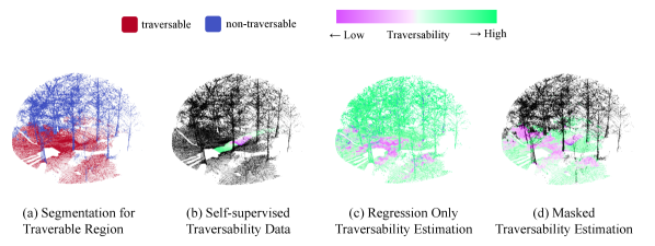
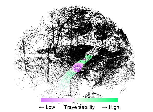
Actual physical state changes that a vehicle undergoes can give meaningful information on where it can traverse and how difficult it would be. Such physical changes that the vehicle encounters itself are called self-supervised data. Accordingly, self-supervised traversability estimation can offer more robot-oriented prediction [11, 12, 13]. Fig. 1b shows an example of the self-supervised traversability data. Previously, haptic inspection [13, 11] has been examined as traversability in the self-supervised approaches. These works demonstrate that learning self-supervised data is a promising approach for traversability estimation, but are only delved into the proprioceptive sensor domain or image domain. Additionally, supervision from the self-supervised data is limited to the actually traversed regions as depicted in Fig. 1b, thereby inducing an epistemic uncertainty when inferring the traversability on non-traversed regions. An example of such epistemic uncertainty is illustrated in Fig. 1c. Trees that are impossible to drive over are regressed with high traversability, which means they are easy to traverse.
In this paper, we propose a self-supervised framework on D point cloud data for traversability estimation in unconstrained environments concentrated on alleviating epistemic uncertainty. We jointly learn semantic segmentation along with traversability regression via deep metric learning to filter out the non-traversable regions (see Fig. 1d.) Also, to harness the unlabeled data from the non-traversed area, we introduce the unsupervised loss similar to the clustering methods [14]. To better evaluate our task, we develop a new evaluation metric that can both evaluate the segmentation and the regression, while highlighting the false-positive ratio for reliable estimation. To test our method on more realistic data, we build an off-road robot driving dataset named ‘Dtrail.’ Experimental results are both shown for Dtrail and SemanticKITTI [15] dataset. Ablations and comparisons with the other metric learning-based methods show that our method yields quantitatively and qualitatively robust results. Our contributions to this work are fivefold:
-
•
We introduce a self-supervised traversability estimation framework on 3D point clouds that mitigates the uncertainty.
-
•
We adopt a deep metric learning-based method that jointly learns the semantic segmentation and the traversability estimation.
-
•
We propose the unsupervised loss to utilize the unlabeled data in the current self-supervised settings.
-
•
We devise a new metric to evaluate the suggested framework properly.
-
•
We present a new 3D point cloud dataset for off-road mobile robot driving in unconstrained environments that includes IMU data synchronized with LiDAR.
II Related Works
II-A Traversability Estimation
Traversability estimation is a crucial component in mobile robotics platforms for estimating where it should go. In the case of paved road conditions, the traversability estimation task can be regarded as a subset of road detection [5, 16] and semantic segmentation [17]. However, the human-supervised method is clearly limited in estimating traversability for unconstrained environments like off-road areas. According to the diversity of the road conditions, it is hard to determine the traversability of a mobile robot in advance by man-made predefined rules.
Self-supervised approaches [18, 19, 20, 13] are suggested in the robotics literature to estimate the traversability using proprioceptive sensors such as inertial measurement and force-torque sensors [13]. Since these tasks only measured traversability in the proprioceptive-sensor domain, they do not affect the robot’s future driving direction. To solve this problem, a study to predict terrain properties by combining image information with the robot’s self-supervision has been proposed [11]. They identify the terrain properties from haptic interaction and associate them with the image to facilitate self-supervised learning. This work demonstrates promising outputs for traversability estimation, but it does not take epistemic uncertainty into account that necessarily exists in the self-supervised data. Furthermore, image data-based learning approaches are still vulnerable to illumination changes that can reduce the performance of the algorithms. Therefore, range sensors such as 3D LiDAR can be a strong alternative [21].
To overcome such limitations, we propose self-supervised traversability estimation in unconstrained environments that can alleviate congenital uncertainty from 3D point cloud data.
II-B Deep Metric Learning
One of the biggest challenges in learning with few labeled data is epistemic uncertainty. To handle this problem, researchers proposed deep metric learning (DML) [22], which learns embedding spaces and classifies an unseen sample in the learned space. Several works adopt the sampled mini-batches called episodes during training, which mimics the task with few labeled data to facilitate DML [23, 24, 25, 26]. These methods with episodic training strategies epitomize labeled data of each class as a single vector, referred to as a prototype [27, 28, 29, 30, 17]. The prototypes generated by these works require non-parametric procedures and insufficiently represent unlabeled data.
Other works [31, 32, 33, 34, 31, 35, 36] develop loss functions to learn an embedding space where similar examples are attracted, and dissimilar examples are repelled. Recently, proxy-based loss [37] is proposed. Proxies are representative vectors of the training data in the learned embedding spaces, which are obtained in a parametric way [38, 39]. Using proxies leads to better convergence as they reflect the entire distribution of the training data [37]. A majority of the works [38, 39] provides a single proxy for each class, whereas SoftTriple loss [40] adopts multiple proxies for each class. We adopt the SoftTriple loss, as traversable and non-traversable regions are represented as multiple clusters rather than a single one in the unstructured driving surfaces according to their complexity and roughness.
III Methods
III-A Overview
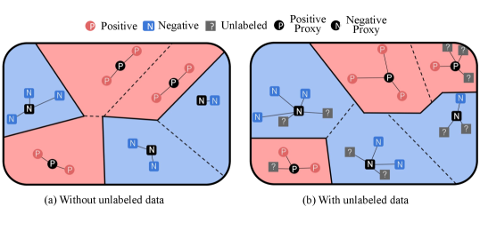
Our self-supervised framework aims to learn a mapping between point clouds to traversability. We call input data containing the traversability information as ‘query.’ The traversable regions are referred to as the ‘positive’ class, and the non-traversable regions are referred to as the ‘negative’ class in this work. In query data, only positive data are labeled along with their traversability. The rest remains as unlabeled regions. Non-black points in Fig. 2(a) indicate the positive regions and the black points indicate the unlabeled regions.
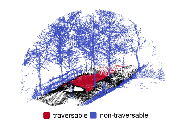
However, there exists a limitation in that the query data is devoid of any supervision about negative regions. With query data only, results would be unreliable, as negative regions can be regressed as a good traversable region due to the epistemic uncertainty (Fig. 1c.) Consequently, our task aims to learn semantic segmentation along with traversability regression to mask out the negative regions, thereby mitigating the epistemic uncertainty. Accordingly, we utilize a very small number of hand-labeled point cloud scenes and call it ‘support’ data. In support data, traversable and non-traversable regions are manually annotated as positive and negative, respectively. Manually labeling entire scenes can be biased with human intuitions. Therefore, only evident regions are labeled and used for training. Fig. 2(b) shows the example of labeled support data.
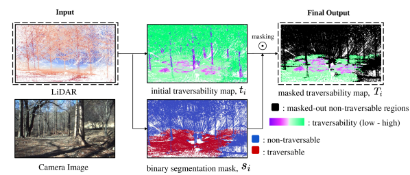
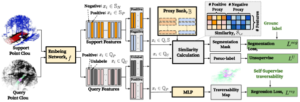
The overall schema of our task is illustrated in Fig. 3. When the input point cloud data is given, a segmentation mask is applied to the initial version of the traversability regression map, producing a masked traversability map as a final output. For training, we form an episode composed of queries and randomly sampled support data. We can optimize our network over both query and relatively small support data with the episodic strategy [17]. Also, to properly evaluate the proposed framework, we introduce a new metric that comprehensively measures the segmentation and the regression, while highlighting the nature of the traversability estimation task with the epistemic uncertainty.
III-B Baseline Method
Let query data, consisting of positive and unlabeled data, as , and support data, consisting of positive and negative data, as . Let denotes the D point, denotes the traversability, and denotes the class of each point. Accordingly, data from , , , and are in forms of , , , and , respectively. Let denote a feature encoding backbone where indicates a network parameter, as encoded features extracted from , and as the multi-layer perceptron (MLP) head for the traversability regression. denotes the MLP head for the segmentation that distinguishes the traversable and non-traversable regions. The encoded feature domain for each data is notated as , , , and .
A baseline solution learns the network with labeled data only. is used for the traversability regression and and are both used for the segmentation. We obtain the traversability map , , and segmentation map . The final masked traversability map is represented as element-wise multiplication, . The regression loss is computed with and based on a mean squared error loss as Eq. (1), where is the -th element of .
| (1) |
For the segmentation loss , binary cross-entropy loss is used in the supervised setting as Eq. (2), where refers to the -th element of either and . Both the positive query and the support data can be used for the segmentation loss as follows:
| (2) |
Combining the regression and the segmentation, the traversability estimation loss in the supervised setting is defined as follows:
| (3) |
Nonetheless, it does not fully take advantage of data captured under various driving surfaces. Since the learning is limited to the labeled data, it can not capture the whole characteristics of the training data. This drawback hinders the capability of the traversability estimation trained in a supervised manner.
III-C Metric learning method
We adopt metric learning to overcome the limitation of the fully-supervised solution. The objectives of metric learning are to learn embedding space and find the representations that epitomize the training data in the learned embedding space. To jointly optimize the embedding network and the representations, we adopt a proxy-based loss [39]. The embedding network is updated based on the positions of the proxies, and the proxies are adjusted by the updated embedding network iteratively. The proxies can be regarded as representations that abstract the training data. We refer this set of proxies as ‘proxy bank,’ denoted as , where and indicate the set of proxies for each class. The segmentation map is inferred based on the similarity between feature vectors and the proxies of each class, as .
The representations of traversable and non-traversable regions exhibit large intra-class variations, where numerous sub-classes exist in each class; flat ground or gravel road for positive, and rocks, trees, or bushes for negative. For the segmentation, we use SoftTriple loss [40] that utilizes multiple proxies for each class. The similarity between and class , denoted as , is defined by a weighted sum of cosine similarity between and {}, where denotes positive or negative, is the number of proxies per class, and is -th proxy in the proxy bank. The weight given to each cosine similarity is proportionate to its value. is defined as follows:
| (4) |
where is a temperature parameter to control the softness of assignments. Soft assignments reduce sensitivity between multiple centers. Note that the norm has been applied to embedding vectors to sustain divergence of magnitude. Then the SoftTriple loss is defined as follows:
| (5) |
where is a hyperparameter for smoothing effect and is a margin. The segmentation loss using the proxy bank can be reformulated using the SoftTriple loss as Eq. (6) and the traversability estimation loss using the proxy bank is defined as Eq. (7).
| (6) |
| (7) |
Unlabeled data, which is abundantly included in self-supervised traversability data, has not been considered in previous works. To enhance the supervision we can extract from the data, we utilize the unlabeled data in the query data in the learning process. The problem is that the segmentation loss cannot be applied to the because no class label exists for them. We assign an auxiliary target for each unlabeled data as clustering [41]. Pseudo class of -th sample is assigned based on the class of the nearest proxy in the embedding space as .
The unsupervised loss for the segmentation, denoted as , is defined as Eq. (8) using the pseudo-class, where is an embedding of -th sample in .
| (8) |
Fig. 4 illustrates the benefit of incorporating unlabeled loss. The embedding network can learn to capture more broad distribution of data, and learned proxies would represent training data better. When unlabeled data features are assigned to the proxies (Fig. 4a,) the embedding space and proxies are updated as Fig. 4b, exhibiting more precise decision boundaries.
Combining the aforementioned objectives altogether, we define our final objective as ‘Traverse Loss,’ and is defined as Eq. (9). The overall high-level schema of the learning procedure is depicted in Fig. 5.
| (9) |
III-D Re-initialization to avoid trivial solutions
Our metric learning method can suffer from sub-optimal solutions, which are induced by empty proxies. Empty proxies indicate the proxies to which none of the data are assigned. Such empty proxies should be redeployed to be a good representation of training data. Otherwise, the model might lose the discriminative power and the bank might include semantically poor representations.
Our intuitive idea to circumvent an empty proxy is to re-initialize the empty proxy with support data features. By updating the empty proxies with support data, the proxy bank can reflect training data that was not effectively captured beforehand. In order to obtain representative feature vectors without noises, number of prototype feature vectors, denoted as and , are estimated using an Expectation-Maximization algorithm [42]. The prototype vectors are cluster centers of support features. We randomly choose the prototype vectors with small perturbations and use them as re-initialized proxies. Algorithm 1 summarizes the overall training procedure of our method.
III-E Traversability Precision Error
We devise a new metric for the proposed framework, ‘Traversability Precision Error’ (TPE). The new metric should be able to comprehensively evaluate the segmentation and the regression while taking the critical aspect of the traversability estimation into account. One of the most important aspects of traversability estimation is to avoid the false-positive of the traversable region, the region that is impossible to traverse but inferred as traversable. If such a region is estimated as traversable, a robot will likely go over that region, resulting in undesirable movements. The impact of the false-positive decreases if they are estimated as less traversable. TPE computes the degree of false-positive of the traversable region, extenuating its impact with the traversability . The TPE is defined as Eq. (10) where , , and denote the number of true negative, false positive, and false negative points of the traversable region, respectively.
| (10) |
IV Experiments
| Dtrail | SemanticKITTI | |||||||||
|---|---|---|---|---|---|---|---|---|---|---|
| mIoU | TPE | mIoU | ||||||||
| ProtoNet [26] | 0.8033 | 0.7515 | 0.5049 | 0.7129 | 0.5624 | 0.3249 | 0.8009 | 0.8040 | 0.7993 | 0.7798 |
| MPTI [17] | 0.6992 | 0.6936 | 0.6390 | 0.6202 | 0.5466 | 0.4995 | 0.8586 | 0.8108 | 0.7531 | 0.7663 |
| Ours (supervised) | 0.9238 | 0.8857 | 0.7779 | 0.8896 | 0.8447 | 0.7345 | 0.8405 | 0.8376 | 0.8338 | 0.8201 |
| Ours (w.o. unlabeled) | 0.8864 | 0.8529 | 0.8461 | 0.8434 | 0.8121 | 0.8164 | 0.8124 | 0.7896 | 0.8049 | 0.7994 |
| Ours (w.o. re-init) | 0.8970 | 0.8771 | 0.7935 | 0.8649 | 0.8163 | 0.7517 | 0.8058 | 0.7895 | 0.8058 | 0.7895 |
| Ours | 0.9338 | 0.9151 | 0.9005 | 0.9067 | 0.8776 | 0.8636 | 0.8652 | 0.8402 | 0.8473 | 0.8973 |
In this section, our method is evaluated with Dtrail dataset for traversability estimation on off-road environments along with SemanticKITTI [15] dataset. Our method is compared to other metric learning methods based on episodic training strategies. Furthermore, we conduct various ablation studies to show the benefits of our method.
IV-A Datasets

IV-A1 Dtrail: Off-road terrain dataset
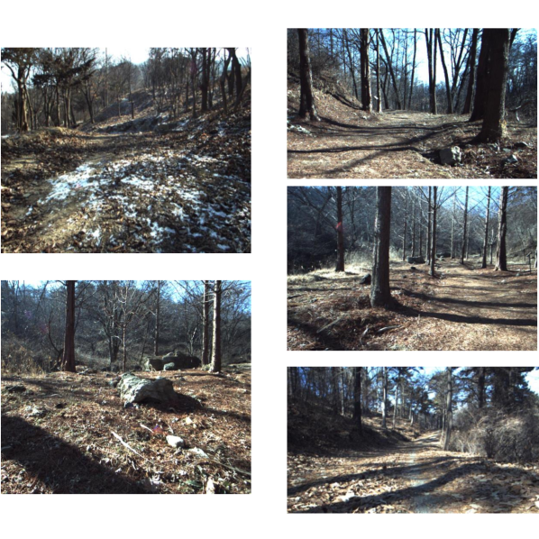
In order to thoroughly examine the validity of our method, we build the Dtrail dataset, a real mobile robot driving dataset of high-resolution LiDAR point clouds from mountain trail scenes. We collect point clouds using one layer and two layers of LiDAR sensors equipped on our caterpillar-type mobile robot platform, shown in Fig. 6(a). Our dataset consists of point cloud scenes and each point cloud scene has approximately million points. Corresponding sample camera images of point cloud scenes are shown in Fig. 6(b). For the experiments, we split scenes for the query set and scenes for the support set, and scenes for the evaluation set. For the traversability, the magnitude z-acceleration from the Inertial Measurement Unit (IMU) of the mobile robot is re-scaled from to and mapped to points that the robot actually explored. Also, in terms of data augmentation, a small perturbation is added along the z-axis on some positive points.
 |
 |
 |
 |
 |
||
| (a) | (b) | (c) | (d) | (e) | ||
| Scene Images | Support Data | Supervised | Ours |
|
IV-A2 SemanticKITTI
We evaluate our method on the SemanticKITTI [15] dataset, which is an urban outdoor-scene dataset for point cloud segmentation. Since it does not provide any type of attributes for traversability, we conducted experiments on segmentation only. It contains sequences, 00 to 10 as the training set, with point clouds and classes. We split sequences (, , , , ) with point clouds for training and the rest, with point clouds, for evaluation. We define the ‘road’, ‘parking’, ‘sidewalk’, ‘other-ground’, and ‘terrain’ classes as positive and the rest classes as negative. For query data, only the ‘road’ class is labeled as positive and left other positive classes as unlabeled. We expect the model to learn the other positive regions using unlabeled data without direct supervision.
IV-B Evaluation metric
We evaluate the performance of our method with TPE, the new criteria designed for the traversability estimation task, which evaluates segmentation and regression quality simultaneously. Additionally, we evaluate the segmentation quality with mean Interaction over Union [43] (mIoU). For each class, the IoU is calculated by , where , , and denote the number of true negatives, false positives, and false negative points of each class, respectively.
IV-C Implementation Details
IV-C1 Embedding network
RandLA-Net [4] is fixed as a backbone embedding network for every method for a fair comparison. Specifically, we use down-sampling layers in the backbone and excluded global positions in the local spatial encoding layer, which aids the network to embed local geometric patterns explicitly. The embedding vectors are normalized with norm and are handled with cosine similarity.
IV-C2 Training
We train the model and proxies with Adam optimizer with the exponential learning rate decay for epochs. The initial learning rate is set as . For query and support data, K-nearest neighbors (KNN) of a randomly picked point is sampled in training steps. We ensure that positive and negative points exist evenly in sampled points of the support data.
IV-C3 Hyperparameter setting
For learning stability, proxies are updated exclusively for the initial epochs. The number of proxies is set to for each class and the proxies are initialized with normal distribution. We set small margin as , as , and temperature parameter as for handling multiple proxies.
IV-D Results
IV-D1 Comparison
We compare the performance to ProtoNet [26] which uses a single prototype and MPTI [17] which adopts multiple prototypes for few-shot 3D segmentation. Also, we compare the performance with our supervised manner method, denoted as ‘Ours(supervised).’ Table I summarizes the result of experiments. Our method shows a significant margin in terms of IoU and TPE compared to the ProtoNet and MPTI. It demonstrates that generating prototypes in a non-parametric approach does not represent the whole data effectively. Moreover, it is notable that we show the performance of our metric learning method is better than the supervised setting designed for our task. It verifies that ours can reduce epistemic uncertainty by incorporating unlabeled data by unsupervised loss. For SemanticKITTI, the observation is similar to that of the Dtrail dataset. Even though the SemanticKITTI dataset is based on urban scenes, our method shows better performance than other few-shot learning methods by and the supervised manner by .
| 1 | 2 | 4 | 8 | 16 | 32 | 64 | 128 | 256 | 512 | |
|---|---|---|---|---|---|---|---|---|---|---|
| mIoU() | 0.890 | 0.894 | 0.880 | 0.906 | 0.911 | 0.883 | 0.920 | 0.934 | 0.931 | 0.924 |
| TPE() | 0.847 | 0.868 | 0.840 | 0.862 | 0.881 | 0.845 | 0.888 | 0.906 | 0.898 | 0.895 |
IV-D2 Ablation studies
We repeat experiments with varying support-to-query ratio () to evaluate robustness regarding the amount of support data. Table I shows that our metric learning method is much more robust from performance degradation than the others when the support-to-query ratio decreases. When the ratio decreases from to in the Dtrail dataset, the TPE of our metric learning method only decreases about while the TPE of others dropped significantly: for ProtoNet, for MPTI, and for Ours(supervised). It verifies that our method can robustly reduce epistemic uncertainty with small labeled data.
Moreover, we observe that performance increases by on average on TPE when adopting the re-initialization step. It confirms the re-initialization step can help avoid trivial solutions. Also, it is shown that adopting the unsupervised loss can boost the performance up to on average. It verifies that the unlabeled loss can give affluent supervision without explicit labels. Moreover, as shown in Table II, an increasing number of proxies boost the performance until it converges when the number exceeds , which demonstrates the advantages of multiple proxies.
IV-D3 Qualitative Results
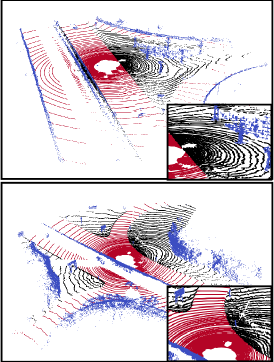
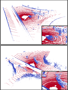
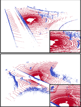
Fig. 7 shows the traversability estimation results of our supervised-based and metric learning-based method on the Dtrail dataset. We can examine that our metric learning-based method performs better than the supervised-based method. Especially, our method yields better results on regions that are not labeled on training data. We compare the example of segmentation results with the SemanticKITTI dataset in Fig. 8. The first column indicates the ground truth and the other columns indicate the segmentation results of the supervised learning-based method and our method. Evidently, our method shows better results on unlabeled regions, which confirms that our metric learning-based method reduces epistemic uncertainty.
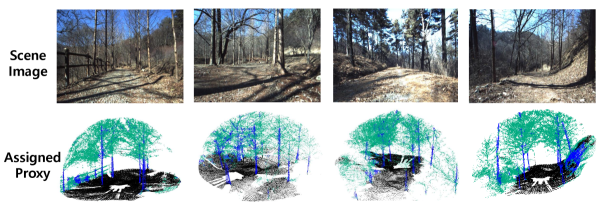
Fig. 9 shows the visualization of the proxies assigned to the point cloud scenes. For better visualization, proxies are clustered into three representations. We observe that the learned proxies successfully represent the various semantic features. Leaves, grounds, and tree trunks are mostly colored green, black, and blue, respectively.
V Conclusion
We propose a self-supervised traversability estimation framework on 3D point cloud data in terms of mitigating epistemic uncertainty. Self-supervised traversability estimation suffers from the uncertainty that arises from the limited supervision given from the data. We tackle the epistemic uncertainty by concurrently learning semantic segmentation along with traversability estimation, eventually masking out the non-traversable regions. We start from the fully-supervised setting and finally developed the deep metric learning method with unsupervised loss that harnessed the unlabeled data. To properly evaluate the framework, we also devise a new evaluation metric according to the task’s settings and underline the important criteria of the traversability estimation. We build our own off-road terrain dataset with the mobile robotics platform in unconstrained environments for realistic testing. Various experimental results show that our framework is promising.
References
- [1] A. Geiger, P. Lenz, C. Stiller, and R. Urtasun, “Vision meets robotics: The kitti dataset,” The International Journal of Robotics Research, vol. 32, pp. 1231 – 1237, 2013.
- [2] H. Caesar, V. Bankiti, A. H. Lang, S. Vora, V. E. Liong, Q. Xu, A. Krishnan, Y. Pan, G. Baldan, and O. Beijbom, “nuscenes: A multimodal dataset for autonomous driving,” IEEE/CVF Conference on Computer Vision and Pattern Recognition, pp. 11 618–11 628, 2020.
- [3] P. Sun, H. Kretzschmar, X. Dotiwalla, A. Chouard, V. Patnaik, P. Tsui, J. Guo, Y. Zhou, Y. Chai, B. Caine, V. Vasudevan, W. Han, J. Ngiam, H. Zhao, A. Timofeev, S. M. Ettinger, M. Krivokon, A. Gao, A. Joshi, Y. Zhang, J. Shlens, Z. Chen, and D. Anguelov, “Scalability in perception for autonomous driving: Waymo open dataset,” IEEE/CVF Conference on Computer Vision and Pattern Recognition, pp. 2443–2451, 2020.
- [4] Q. Hu, B. Yang, L. Xie, S. Rosa, Y. Guo, Z. Wang, A. Trigoni, and A. Markham, “Randla-net: Efficient semantic segmentation of large-scale point clouds,” IEEE/CVF Conference on Computer Vision and Pattern Recognition, pp. 11 105–11 114, 2020.
- [5] Z. Chen, J. Zhang, and D. Tao, “Progressive lidar adaptation for road detection,” IEEE/CAA Journal of Automatica Sinica, vol. 6, pp. 693–702, 2019.
- [6] J. Sock, J. H. Kim, J. Min, and K. H. Kwak, “Probabilistic traversability map generation using 3d-lidar and camera,” IEEE International Conference on Robotics and Automation, pp. 5631–5637, 2016.
- [7] J. Ahtiainen, T. Stoyanov, and J. Saarinen, “Normal distributions transform traversability maps: Lidar‐only approach for traversability mapping in outdoor environments,” Journal of Field Robotics, vol. 34, 2017.
- [8] S. Matsuzaki, J. Miura, and H. Masuzawa, “Semantic-aware plant traversability estimation in plant-rich environments for agricultural mobile robots,” ArXiv, vol. abs/2108.00759, 2021.
- [9] T. Guan, Z. He, D. Manocha, and L. Zhang, “Ttm: Terrain traversability mapping for autonomous excavator navigation in unstructured environments,” ArXiv, vol. abs/2109.06250, 2021.
- [10] H. Roncancio, M. Becker, A. Broggi, and S. Cattani, “Traversability analysis using terrain mapping and online-trained terrain type classifier,” IEEE Intelligent Vehicles Symposium Proceedings, pp. 1239–1244, 2014.
- [11] L. Wellhausen, A. Dosovitskiy, R. Ranftl, K. Walas, C. Cadena, and M. Hutter, “Where should i walk? predicting terrain properties from images via self-supervised learning,” IEEE Robotics and Automation Letters, vol. 4, pp. 1509–1516, 2019.
- [12] M. Wermelinger, P. Fankhauser, R. Diethelm, P. Krüsi, R. Y. Siegwart, and M. Hutter, “Navigation planning for legged robots in challenging terrain,” IEEE/RSJ International Conference on Intelligent Robots and Systems, pp. 1184–1189, 2016.
- [13] H. Kolvenbach, C. Bärtschi, L. Wellhausen, R. Grandia, and M. Hutter, “Haptic inspection of planetary soils with legged robots,” IEEE Robotics and Automation Letters, vol. 4, pp. 1626–1632, 2019.
- [14] W. Van Gansbeke, S. Vandenhende, S. Georgoulis, M. Proesmans, and L. Van Gool, “Scan: Learning to classify images without labels,” in European Conference on Computer Vision, 2020, pp. 268–285.
- [15] J. Behley, M. Garbade, A. Milioto, J. Quenzel, S. Behnke, C. Stachniss, and J. Gall, “Semantickitti: A dataset for semantic scene understanding of lidar sequences,” IEEE/CVF International Conference on Computer Vision, pp. 9296–9306, 2019.
- [16] A. Valada, J. Vertens, A. Dhall, and W. Burgard, “Adapnet: Adaptive semantic segmentation in adverse environmental conditions,” IEEE International Conference on Robotics and Automation, pp. 4644–4651, 2017.
- [17] N. Zhao, T.-S. Chua, and G. H. Lee, “Few-shot 3d point cloud semantic segmentation,” IEEE/CVF Conference on Computer Vision and Pattern Recognition, pp. 8869–8878, 2021.
- [18] P. Dallaire, K. Walas, P. Giguère, and B. Chaib-draa, “Learning terrain types with the pitman-yor process mixtures of gaussians for a legged robot,” IEEE/RSJ International Conference on Intelligent Robots and Systems, pp. 3457–3463, 2015.
- [19] L. Ding, H. Gao, Z. Deng, J. Song, Y. Liu, G. Liu, and K. Iagnemma, “Foot–terrain interaction mechanics for legged robots: Modeling and experimental validation,” The International Journal of Robotics Research, vol. 32, pp. 1585 – 1606, 2013.
- [20] W. Bosworth, J. Whitney, S. Kim, and N. Hogan, “Robot locomotion on hard and soft ground: Measuring stability and ground properties in-situ,” IEEE International Conference on Robotics and Automation, pp. 3582–3589, 2016.
- [21] G. G. Waibel, T. Löw, M. Nass, D. Howard, T. Bandyopadhyay, and P. V. K. Borges, “How rough is the path? terrain traversability estimation for local and global path planning,” IEEE Transactions on Intelligent Transportation Systems, vol. 23, no. 9, p. 16462–16473, sep 2022. [Online]. Available: https://doi.org/10.1109/TITS.2022.3150328
- [22] G. Koch, R. Zemel, R. Salakhutdinov et al., “Siamese neural networks for one-shot image recognition,” in ICML deep learning workshop, vol. 2. Lille, 2015, p. 0.
- [23] V. G. Satorras and J. Bruna, “Few-shot learning with graph neural networks,” ArXiv, vol. abs/1711.04043, 2018.
- [24] O. Vinyals, C. Blundell, T. P. Lillicrap, K. Kavukcuoglu, and D. Wierstra, “Matching networks for one shot learning,” in Advances in Neural Information Processing Systems, 2016.
- [25] F. Sung, Y. Yang, L. Zhang, T. Xiang, P. H. S. Torr, and T. M. Hospedales, “Learning to compare: Relation network for few-shot learning,” IEEE/CVF Conference on Computer Vision and Pattern Recognition, pp. 1199–1208, 2018.
- [26] J. Snell, K. Swersky, and R. S. Zemel, “Prototypical networks for few-shot learning,” ArXiv, vol. abs/1703.05175, 2017.
- [27] C. Chen, O. Li, A. J. Barnett, J. Su, and C. Rudin, “This looks like that: deep learning for interpretable image recognition,” ArXiv, vol. abs/1806.10574, 2019.
- [28] J. Deuschel, D. Firmbach, C. I. Geppert, M. Eckstein, A. Hartmann, V. Bruns, P. Kuritcyn, J. Dexl, D. Hartmann, D. Perrin, T. Wittenberg, and M. Benz, “Multi-prototype few-shot learning in histopathology,” IEEE/CVF International Conference on Computer Vision Workshops, pp. 620–628, 2021.
- [29] K. R. Allen, E. Shelhamer, H. Shin, and J. B. Tenenbaum, “Infinite mixture prototypes for few-shot learning,” ArXiv, vol. abs/1902.04552, 2019.
- [30] B. Yang, C. Liu, B. Li, J. Jiao, and Q. Ye, “Prototype mixture models for few-shot semantic segmentation,” ArXiv, vol. abs/2008.03898, 2020.
- [31] F. Schroff, D. Kalenichenko, and J. Philbin, “Facenet: A unified embedding for face recognition and clustering,” IEEE Conference on Computer Vision and Pattern Recognition, pp. 815–823, 2015.
- [32] M. Wang and W. Deng, “Deep face recognition: A survey,” Neurocomputing, vol. 429, pp. 215–244, 2021.
- [33] S. Chopra, R. Hadsell, and Y. LeCun, “Learning a similarity metric discriminatively, with application to face verification,” IEEE Computer Society Conference on Computer Vision and Pattern Recognition, vol. 1, pp. 539–546 vol. 1, 2005.
- [34] R. Hadsell, S. Chopra, and Y. LeCun, “Dimensionality reduction by learning an invariant mapping,” IEEE Computer Society Conference on Computer Vision and Pattern Recognition, vol. 2, pp. 1735–1742, 2006.
- [35] J. Wang, Y. Song, T. Leung, C. Rosenberg, J. Wang, J. Philbin, B. Chen, and Y. Wu, “Learning fine-grained image similarity with deep ranking,” IEEE Conference on Computer Vision and Pattern Recognition, pp. 1386–1393, 2014.
- [36] H. O. Song, Y. Xiang, S. Jegelka, and S. Savarese, “Deep metric learning via lifted structured feature embedding,” IEEE Conference on Computer Vision and Pattern Recognition, pp. 4004–4012, 2016.
- [37] Y. Movshovitz-Attias, A. Toshev, T. Leung, S. Ioffe, and S. Singh, “No fuss distance metric learning using proxies,” IEEE International Conference on Computer Vision, pp. 360–368, 2017.
- [38] E. W. Teh, T. Devries, and G. W. Taylor, “Proxynca++: Revisiting and revitalizing proxy neighborhood component analysis,” ArXiv, vol. abs/2004.01113, 2020.
- [39] S. Kim, D. Kim, M. Cho, and S. Kwak, “Proxy anchor loss for deep metric learning,” IEEE/CVF Conference on Computer Vision and Pattern Recognition, pp. 3235–3244, 2020.
- [40] Q. Qian, L. Shang, B. Sun, J. Hu, H. Li, and R. Jin, “Softtriple loss: Deep metric learning without triplet sampling,” IEEE/CVF International Conference on Computer Vision, pp. 6449–6457, 2019.
- [41] M. Caron, P. Bojanowski, A. Joulin, and M. Douze, “Deep clustering for unsupervised learning of visual features,” in European Conference on Computer Vision, 2018.
- [42] T. K. Moon, “The expectation-maximization algorithm,” IEEE Signal processing magazine, vol. 13, no. 6, pp. 47–60, 1996.
- [43] M. Everingham, L. V. Gool, C. K. I. Williams, J. M. Winn, and A. Zisserman, “The pascal visual object classes (voc) challenge,” International Journal of Computer Vision, vol. 88, pp. 303–338, 2009.