This paper was converted on www.awesomepapers.org from LaTeX by an anonymous user.
Want to know more? Visit the Converter page.

Self-triggered Consensus of Multi-agent Systems with Quantized Relative State Measurements

Masashi Wakaiki Graduate School of System Informatics, Kobe University, Nada, Kobe, Hyogo 657-8501, Japan wakaiki@ruby.kobe-u.ac.jp
Abstract.

This paper addresses the consensus problem of first-order continuous-time multi-agent systems over undirected graphs. Each agent samples relative state measurements in a self-triggered fashion and transmits the sum of the measurements to its neighbors. Moreover, we use finite-level dynamic quantizers and apply the zooming-in technique. The proposed joint design method for quantization and self-triggered sampling achieves asymptotic consensus, and inter-event times are strictly positive. Sampling times are determined explicitly with iterative procedures including the computation of the Lambert WW-function. A simulation example is provided to illustrate the effectiveness of the proposed method.

This work was supported by JSPS KAKENHI Grant Number JP20K14362.

1. Introduction

With the recent development of information and communication technologies, multi-agent systems have received considerable attention. Cooperative control of multi-agent systems can be applied to various areas such as multi-vehicle formulation [1] and distributed sensor networks [2]. A basic coordination problem of multi-agent systems is consensus, whose aim is to reach an agreement on the states of all agents. A theoretical framework for consensus problems has been introduced in the seminal work [3], and substantial progress has been made since then; see the survey papers [4, 5] and the references therein.

In practice, digital devices are used in multi-agent systems. Conventional approaches to implementing digital platforms involve periodic sampling. However, periodic sampling can lead to unnecessary control updates and state measurements, which are undesirable for resource-constrained multi-agent systems. Event-triggered control [6, 7, 8] and self-triggered control [9, 10, 11] are promising alternatives to traditional periodic control. In both event-triggered and self-triggered control systems, data transmissions and control updates occur only when needed. Event-triggering mechanisms use current measurements and check triggering conditions continuously or periodically. On the other hand, self-triggering mechanisms avoid such frequent monitoring by calculating the next sampling time when data are obtained. Various methods have been developed for event-triggered consensus and self-triggered consensus; see, e.g., [12, 13, 14, 15, 16]. Comprehensive surveys on this topic are available in [17, 18]. Some specifically relevant studies are cited below.

The bandwidth of communication channels and the accuracy of sensors may be limited in multi-agent systems. In such situations, only imperfect information is available to the agents. We also face the theoretical question of how much accuracy in information is necessary for consensus. From both practical and theoretical point of view, quantized consensus has been studied extensively. For continuous-time multi-agent systems, infinite-level static quantization is often considered under the situation where quantized measurements are obtained continuously; see, e.g., [19, 20, 21, 22, 23, 24, 25]. Event-triggering mechanisms and self-triggering mechanisms have been proposed for continuous-time multi-agent systems with infinite-level static quantizers in [26, 27, 28, 29, 30, 31, 32, 33, 34, 35]. Self-triggered consensus with ternary controllers has been also studied in [36, 37]. For event-triggered consensus under unknown input delays, finite-level dynamic quantizers have been developed in [38], where the quantization error goes to zero as the agent state converges to the origin.

For discrete-time multi-agent systems, finite-level dynamic quantizers to achieve asymptotic consensus have been designed in [39, 40, 41, 42, 43]. This type of dynamic quantization has been also used for periodic sampled-data consensus [44], event-triggered consensus [45, 46, 47, 48, 49], and consensus under denial-of-service attacks [50]. Moreover, an event-triggered average consensus protocol has been proposed for discrete-time multi-agent systems with integer-valued states in [51], and it has been extended to the privacy-preserving case in [52].

In this paper, we consider first-order continuous-time multi-agent systems over undirected graphs. Our goal is to jointly design a finite-level dynamic quantizer and a self-triggering mechanism for asymptotic consensus. We focus on the situation where relative states, not absolute states, are sampled as, e.g., in [16, 19, 22, 30, 29, 24, 31, 32, 34]. We assume that each agent’s sensor has a scaling parameter to adjust the maximum measurement range and the accuracy. For example, if indirect time-of-flight sensors [53] are installed in agents, then the modulation frequency of light signals determines the maximum range and the accuracy. In the case of cameras, they can be changed by adjusting the focal length; see Section 11.2 of [54] for a mathematical model of cameras.

In the proposed self-triggered framework, the agents send the sum of the relative state measurements to all their neighbors as in the self-triggered consensus algorithm presented in [14]. In other words, each agent communicates with its neighbors only at the sampling times of itself and its neighbors. The sum is transmitted so that the neighbors compute the next sampling times, not the inputs. After receiving it, the neighbors update the next sampling times. Since the measurements are already quantized when they are sampled, the sum can be transmitted without error, even over channels with finite capacity.

The main contributions of this paper are summarized as follows:

1. We propose a joint algorithm for finite-level dynamic quantization and self-triggered sampling of the relative states. We also provide a sufficient condition for the consensus of the quantized self-triggered multi-agent system. This sufficient condition represents a quantitative trade-off between data accuracy and sampling frequency. Such a trade-off can be a useful guideline for sensing performance, power consumption, and channel capacity.

2. In the proposed method, the inter-event times, i.e., the sampling intervals of each agent, are strictly positive, and hence Zeno behavior does not occur. In addition, the agents can compute sampling times using an explicit formula with the Lambert WW-function (see, e.g., [55] for the Lambert WW-function). Consequently, the proposed self-triggering mechanism is simple and efficient in computation.

We now compare our results with previous studies. The finite-level dynamic quantizers developed in [39, 40, 41, 42, 43] and their aforementioned extensions require the absolute states. More specifically, they quantize the error between the absolute state and its estimate for communication over finite-capacity channels. In this framework, the agents have to estimate the states of all their neighbors for decoding. In contrast, we develop finite-level dynamic quantizers for relative state measurements. As in the existing studies above, we also employ the zooming-in technique introduced for single-loop systems in [56, 57]. However, due to the above-mentioned difference in what is quantized, the quantizer we study has several notable features. For example, the proposed algorithm can be applied to GPS-denied environments. Moreover, the estimation of neighbor states is not needed, which reduces the computational burden on the agents.

A finite-level quantizer may be saturated, i.e., it does not guarantee the accuracy of quantized data in general if the original data is outside of the quantization region. To achieve asymptotic consensus, we need to update the scaling parameter of the quantizer so that the relative state measurement is within the quantization region and the quantization error goes to zero asymptotically. In [29, 32, 34], infinite-level static quantizers have been used for quantized self-triggered consensus of first-order multi-agent systems. Hence the issue of quantizer saturation has not been addressed there. In [29], infinite-level uniform quantization has been considered, and consequently only consensus to a bounded region around the average of the agent states has been achieved. The quantized self-triggered control algorithm proposed in [32, 34] achieves asymptotic consensus with the help of infinite-level logarithmic quantizers, but sampling times have to belong to the set {t=kh:k is a nonnegative integer}\{t=kh:\text{$k$ is a nonnegative integer}\} with some h>0h>0, which makes it easy to exclude Zeno behavior. Table 1 summarizes the comparison between this study and several relevant studies.

The difficulty of this study is that the following three conditions must be satisfied:

  • avoiding quantizer saturation;

  • decreasing the quantization error asymptotically; and

  • guaranteeing that the inter-event times are strictly positive.

To address this difficulty, we introduce a new semi-norm ||||||{|\kern-1.07639pt|\kern-1.07639pt|\cdot|\kern-1.07639pt|\kern-1.07639pt|}_{\infty} for the analysis of multi-agent systems. The semi-norm is constructed from the maximum norm and is suitable for handling errors of individual agents due to quantization and self-triggered sampling. Moreover, the Laplacian matrix LN×NL\in\mathbb{R}^{N\times N} of the multi-agent system has the following semi-contractivity property: There exists a constant γ>0\gamma>0 such that

|eLtv|eγt|v|{|\kern-1.07639pt|\kern-1.07639pt|e^{-Lt}v|\kern-1.07639pt|\kern-1.07639pt|}_{\infty}\leq e^{-\gamma t}{|\kern-1.07639pt|\kern-1.07639pt|v|\kern-1.07639pt|\kern-1.07639pt|}_{\infty}

for all vNv\in\mathbb{R}^{N} and t0t\geq 0; see [58, 59] for the semi-contraction theory. The semi-contractivity property facilitates the analysis of state trajectories under self-triggered sampling and consequently leads to a simple design of the scaling parameter for finite-level dynamic quantization.

Table 1. Comparison between this study and several relevant studies.
Triggering mechanism Measurement Quantization Agent dynamics
This study Self-trigger Relative state Finite-level & dynamic First-order
[38, 46, 47, 48, 49] Event-trigger Absolute state Finite-level & dynamic High-order
[29, 32, 34] Self-trigger Relative state Infinite-level & static First-order

The rest of this paper is organized as follows. In Section 2, we introduce the system model. In Section 3, we provide some preliminaries on the semi-norm and sampling times. Section 4 contains the main result, which gives a sufficient condition for consensus. In Section 5, we explain how the agents compute sampling times in a self-triggered fashion. A simulation example is given in Section 6, and Section 7 concludes this paper.

Notation: We denote the set of nonnegative integers by 0\mathbb{N}_{0}. We define inf\inf\emptyset\coloneqq\infty. Let M,NM,N\in\mathbb{N}. We denote the transpose of AM×NA\in\mathbb{R}^{M\times N} by AA^{\top}. For a vector vNv\in\mathbb{R}^{N} with the ii-th element viv_{i}, its maximum norm is

vmax{|v1|,,|vN|},\|v\|_{\infty}\coloneqq\max\{|v_{1}|,\dots,|v_{N}|\},

and the corresponding induced norm of AM×NA\in\mathbb{R}^{M\times N} with the (i,j)(i,j)-th element AijA_{ij} is given by

A=max{j=1N|Aij|:1iM}.\|A\|_{\infty}=\max\left\{\sum_{j=1}^{N}|A_{ij}|:1\leq i\leq M\right\}.

When the eigenvalues λ1,λ2,,λN\lambda_{1},\lambda_{2},\cdots,\lambda_{N}\in\mathbb{R} of a symmetric matrix PN×NP\in\mathbb{R}^{N\times N} with N2N\geq 2 satisfy λ1λ2λN\lambda_{1}\leq\lambda_{2}\leq\cdots\leq\lambda_{N}, we write λ2(P)λ2\lambda_{2}(P)\coloneqq\lambda_{2}. We define

𝟏[111]N,𝟏¯1N𝟏\mathbf{1}\coloneqq\begin{bmatrix}1&1&\cdots&1\end{bmatrix}^{\top}\in\mathbb{R}^{N},\qquad\bar{\mathbf{1}}\coloneqq\frac{1}{N}\mathbf{1}^{\top}

and write ave(v)𝟏¯v\mathrm{ave}(v)\coloneqq\bar{\mathbf{1}}v for vNv\in\mathbb{R}^{N}. The graph Laplacian of an undirected graph GG is denoted by L(G)L(G). We denote the Lambert WW-function by W(y)W(y) for y0y\geq 0. In other words, W(y)W(y) is the solution x0x\geq 0 of the transcendental equation xex=yxe^{x}=y. Throughout this paper, we shall use the following fact frequently without comment: For a,ω>0a,\omega>0 and cc\in\mathbb{R}, the solution x=xx=x^{*} of the transcendental equation a(xc)=eωxa(x-c)=e^{-\omega x} can be written as

x=1ωW(ωeωca)+c.x^{*}=\frac{1}{\omega}W\left(\frac{\omega e^{-\omega c}}{a}\right)+c.

2. System Model

2.1. Multi-agent system

Let NN\in\mathbb{N} be N2N\geq 2, and consider a multi-agent system with NN agents. Each agent has a label i𝒩{1,2,,N}i\in\mathcal{N}\coloneqq\{1,2,\dots,N\}. For every i𝒩i\in\mathcal{N}, the dynamics of agent ii is given by

(1) x˙i(t)=ui(t),t0;xi(0)=xi0,\dot{x}_{i}(t)=u_{i}(t),\quad t\geq 0;\qquad x_{i}(0)=x_{i0}\in\mathbb{R},

where xi(t)x_{i}(t)\in\mathbb{R} and ui(t)u_{i}(t)\in\mathbb{R} are the state and the control input of agent ii, respectively. The network topology of the multi-agent system is given by a fixed undirected graph G=(𝒱,)G=(\mathcal{V},\mathcal{E}) with vertex set 𝒱={v1,v2,,vN}\mathcal{V}=\{v_{1},v_{2},\dots,v_{N}\} and edge set

{(vi,vj)𝒱×𝒱:ij}.\mathcal{E}\subseteq\{(v_{i},v_{j})\in\mathcal{V}\times\mathcal{V}:i\not=j\}.

If (vi,vj)(v_{i},v_{j})\in\mathcal{E}, then agent jj is called a neighbor of agent ii, and these two agents can measure the relative states and communicate with each other. For i𝒩i\in\mathcal{N}, we denote by 𝒩i\mathcal{N}_{i} the set of all neighbors of agent ii and by did_{i} the degree of the node viv_{i}, that is, the cardinality of the set 𝒩i\mathcal{N}_{i}.

Consider the ideal case without quantization or self-triggered sampling, and set

(2) ui(t)=j𝒩i(xi(t)xj(t))u_{i}(t)=-\sum_{j\in\mathcal{N}_{i}}\big{(}x_{i}(t)-x_{j}(t)\big{)}

for t0t\geq 0 and i𝒩i\in\mathcal{N}. It is well known that the multi-agent system to which the control input (2) is applied achieves average consensus under the following assumption.

Assumption 2.1.

The undirected graph GG is connected.

In this paper, we place Assumption 2.1. Moreover, we make two assumptions, which are used to avoid the saturation of quantization schemes. These assumptions are relative-state analogues of the assumptions in the previous studies on quantized consensus based on absolute state measurements (see, e.g., Assumptions 3 and 4 of [44]).

Assumption 2.2.

A bound E0>0E_{0}>0 satisfying

|xi01Nj𝒩xj0|E0for all i𝒩\left|x_{i0}-\frac{1}{N}\sum_{j\in\mathcal{N}}x_{j0}\right|\leq E_{0}\qquad\text{for all~{}}i\in\mathcal{N}

is known by all agents.

Assumption 2.3.

A bound d~\tilde{d}\in\mathbb{N} satisfying

did~for all i𝒩d_{i}\leq\tilde{d}\qquad\text{for all~{}}i\in\mathcal{N}

is known by all agents.

We make an assumption on the number RR of quantization levels.

Assumption 2.4.

The number RR of quantization levels is an odd number, i.e., R=2R0+1R=2R_{0}+1 for some R00R_{0}\in\mathbb{N}_{0}.

In this paper, we study the following notion of consensus of multi-agent systems under Assumption 2.2.

Definition 2.5.

The multi-agent system achieves consensus exponentially with decay rate ω>0\omega>0 under Assumption 2.2 if there exists a constant Ω>0\Omega>0, independent of E0E_{0}, such that

(3) |xi(t)xj(t)|ΩE0eωt|x_{i}(t)-x_{j}(t)|\leq\Omega E_{0}e^{-\omega t}

for all t0t\geq 0 and i,j𝒩i,j\in\mathcal{N}.

2.2. Quantization scheme

Let E>0E>0 be a quantization range and let RR\in\mathbb{N} be the number of quantization levels satisfying Assumption 2.4. We assume that EE and RR are shared among all agents. We apply uniform quantization to the interval [E,E][-E,E]. Namely, a quantization function QE,RQ_{E,R} is defined by

QE,R[z]{2pERif (2p1)ER<z(2p+1)ER0if ERzERQE,R[z]if z<ERQ_{E,R}[z]\coloneqq\begin{cases}\dfrac{2pE}{R}&\text{if $\dfrac{(2p-1)E}{R}<z\leq\dfrac{(2p+1)E}{R}$}\vspace{8pt}\\ 0&\text{if $-\dfrac{E}{R}\leq z\leq\dfrac{E}{R}$}\vspace{8pt}\\ -Q_{E,R}[-z]&\text{if $z<-\dfrac{E}{R}$}\end{cases}

for z[E,E]z\in[-E,E], where pp\in\mathbb{N} and pR0p\leq R_{0}. By construction,

|zQE,R[z]|ER\big{|}z-Q_{E,R}[z]\big{|}\leq\frac{E}{R}

for all z[E,E]z\in[-E,E]. The agents use a fixed RR but change EE in order to achieve consensus asymptotically. In other words, EE is the scaling parameter of the quantization scheme.

Let {tki}k0\{t_{k}^{i}\}_{k\in\mathbb{N}_{0}} be a strictly increasing sequence with t0i0t_{0}^{i}\coloneqq 0, and tkit_{k}^{i} is the kk-th sampling time of agent ii. To describe the quantized data used at time t=tkit=t_{k}^{i} for k0k\in\mathbb{N}_{0}, we assume for the moment that a certain function E:[0,)(0,)E:[0,\infty)\to(0,\infty) satisfies the unsaturation condition

(4) |xi(tki)xj(tki)|E(tki)for all j𝒩i.|x_{i}(t_{k}^{i})-x_{j}(t_{k}^{i})|\leq E(t_{k}^{i})\quad\text{for all $j\in\mathcal{N}_{i}$}.

Agent ii measures the relative state xi(tki)xj(tki)x_{i}(t_{k}^{i})-x_{j}(t_{k}^{i}) for each neighbor j𝒩ij\in\mathcal{N}_{i} and obtains its quantized value

qij(tki)QE(tki),R[xi(tki)xj(tki)].q_{ij}(t_{k}^{i})\coloneqq Q_{E(t_{k}^{i}),R}[x_{i}(t_{k}^{i})-x_{j}(t_{k}^{i})].

Then agent ii sends to each neighbor j𝒩ij\in\mathcal{N}_{i} the sum

qi(tki)j𝒩iqij(tki).q_{i}(t_{k}^{i})\coloneqq\sum_{j\in\mathcal{N}_{i}}q_{ij}(t_{k}^{i}).

The neighbors use the sum qi(tki)q_{i}(t_{k}^{i}) to calculate the next sampling time, not the input. This data transmission implies that the agents use information not only about direct neighbors but also about two-hop neighbors as in the self-triggering mechanism developed in [14].

The sum qi(tki)q_{i}(t_{k}^{i}) consists of the quantized values, and therefore agent ii can transmit qi(tki)q_{i}(t_{k}^{i}) without errors even through finite-capacity channels. In fact, since RR is an odd number under Assumption 2.4, the sum qi(tki)q_{i}(t_{k}^{i}) belongs to the finite set

{2pE(tki)R:p and d~R0pd~R0},\left\{\frac{2pE(t_{k}^{i})}{R}:p\in\mathbb{Z}\text{~{}~{}~{}and~{}~{}}-\tilde{d}R_{0}\leq p\leq\tilde{d}R_{0}\right\},

where d~\tilde{d}\in\mathbb{N} is as in Assumption 2.3. The encoder of agent ii assigns an index to each value 2pE/R2pE/R and transmits the index corresponding to the sum qi(tki)q_{i}(t_{k}^{i}) to the decoder of each neighbor j𝒩ij\in\mathcal{N}_{i}. Since the agents share EE, RR, and d~\tilde{d}, the decoder can generate the sum qi(tki)q_{i}(t_{k}^{i}) from the received index.

2.3. Triggering mechanism

Let a strictly increasing sequence {tki}k0\{t_{k}^{i}\}_{k\in\mathbb{N}_{0}} with t0i0t_{0}^{i}\coloneqq 0 be the sampling times of agent i𝒩i\in\mathcal{N} as in Section 2.2, and let k0k\in\mathbb{N}_{0}. As in the ideal case (2), the control input ui(t)u_{i}(t) of agent ii is given by the sum of the quantized relative state,

(5) ui(t)=qi(tki)=j𝒩iQE(tki),R[xi(tki)xj(tki)],u_{i}(t)=-q_{i}(t_{k}^{i})=-\sum_{j\in\mathcal{N}_{i}}Q_{E(t_{k}^{i}),R}[x_{i}(t_{k}^{i})-x_{j}(t_{k}^{i})],

for tkit<tk+1it_{k}^{i}\leq t<t_{k+1}^{i} when the unsaturation condition (4) is satisfied. Then the dynamics of agent ii can be written as

(6) x˙i(t)=j𝒩i(xi(t)xj(t))+fi(t)+gi(t),\displaystyle\dot{x}_{i}(t)=-\sum_{j\in\mathcal{N}_{i}}\big{(}x_{i}(t)-x_{j}(t)\big{)}+f_{i}(t)+g_{i}(t),

where fi(t)f_{i}(t) and gi(t)g_{i}(t) are, respectively, the errors due to sampling and quantization defined by

(7) fi(t)\displaystyle f_{i}(t) j𝒩i(xi(t)xj(t))j𝒩i(xi(tki)xj(tki))\displaystyle\coloneqq\sum_{j\in\mathcal{N}_{i}}\big{(}x_{i}(t)-x_{j}(t)\big{)}-\sum_{j\in\mathcal{N}_{i}}\big{(}x_{i}(t_{k}^{i})-x_{j}(t_{k}^{i})\big{)}
(8) gi(t)\displaystyle g_{i}(t) j𝒩i(xi(tki)xj(tki))qi(tki)\displaystyle\coloneqq\sum_{j\in\mathcal{N}_{i}}\big{(}x_{i}(t_{k}^{i})-x_{j}(t_{k}^{i})\big{)}-q_{i}(t_{k}^{i})

for tkit<tk+1it_{k}^{i}\leq t<t_{k+1}^{i}.

We make a triggering condition on the error fif_{i} due to sampling. From the dynamics (1) and the input (5) of each agent, we have that for all tkit<tk+1it_{k}^{i}\leq t<t_{k+1}^{i},

(9) xi(t)xi(tki)\displaystyle x_{i}(t)-x_{i}(t_{k}^{i}) =tkitui(s)𝑑s=(ttki)qi(tki)\displaystyle=\int_{t_{k}^{i}}^{t}u_{i}(s)ds=-(t-t_{k}^{i})q_{i}(t_{k}^{i})
(10) xj(t)xj(tki)\displaystyle x_{j}(t)-x_{j}(t_{k}^{i}) =tkituj(s)𝑑s.\displaystyle=\int_{t_{k}^{i}}^{t}u_{j}(s)ds.

Substituting (9) and (10) into (7) motivates us to consider the following function obtained only from the inputs:

fki(τ)\displaystyle f_{k}^{i}(\tau) j𝒩itkitki+τ(ui(s)uj(s))𝑑s\displaystyle\coloneqq\sum_{j\in\mathcal{N}_{i}}\int_{t_{k}^{i}}^{t_{k}^{i}+\tau}\big{(}u_{i}(s)-u_{j}(s)\big{)}ds
(11) =τdiqi(tki)j𝒩itkitki+τuj(s)𝑑s\displaystyle=-\tau d_{i}q_{i}(t_{k}^{i})-\sum_{j\in\mathcal{N}_{i}}\int_{t_{k}^{i}}^{t_{k}^{i}+\tau}u_{j}(s)ds

for τ0\tau\geq 0. Notice that

fi(tki+τ)=fki(τ)f_{i}(t_{k}^{i}+\tau)=f_{k}^{i}(\tau)

for all τ[0,tk+1itki)\tau\in[0,t_{k+1}^{i}-t_{k}^{i}). Using the quantization range E(t)E(t), we define the (k+1)(k+1)-th sampling time tk+1it_{k+1}^{i} of agent i𝒩i\in\mathcal{N} by

(12) {tk+1itki+min{τki,τmaxi}τkiinf{ττmini:|fki(τ)|δiE(tki+τ)},\left\{\begin{aligned} t_{k+1}^{i}&\coloneqq t_{k}^{i}+\min\{\tau_{k}^{i},\,\tau^{i}_{\max}\}\\ \tau_{k}^{i}&\coloneqq\inf\{\tau\geq\tau^{i}_{\min}:|f_{k}^{i}(\tau)|\geq\delta_{i}E(t_{k}^{i}+\tau)\},\end{aligned}\right.

where δi>0\delta_{i}>0 is a threshold and τmaxi,τmini>0\tau^{i}_{\max},\tau^{i}_{\min}>0 are upper and lower bounds of inter-event times, respectively, i.e., τminiτkiτmaxi\tau^{i}_{\min}\leq\tau_{k}^{i}\leq\tau^{i}_{\max}.

The behaviors of the errors fi(t)f_{i}(t) and gi(t)g_{i}(t) can be roughly described as follows. Under the triggering mechanism (12), the error |fi(t)||f_{i}(t)| due to sampling is upper-bounded by δiE(t)\delta_{i}E(t). The error |gi(t)||g_{i}(t)| due to quantization is also bounded from above by a constant multiple of E(tki)E(t_{k}^{i}) for tkit<tk+1it_{k}^{i}\leq t<t_{k+1}^{i} when the quantizer is not saturated. Hence, if E(t)E(t) decreases to zero as tt\to\infty, then both errors fi(t)f_{i}(t) and gi(t)g_{i}(t) also go to zero.

After some preliminaries in Section 3, Section 4 is devoted to finding a quantization range E(t)E(t), a threshold δi\delta_{i}, and upper and lower bounds τmaxi,τmini\tau^{i}_{\max},\tau^{i}_{\min} of inter-event times such that consensus (3) as well as the unsaturation condition (4) are satisfied. In Section 5, we present a method for agent ii to compute the sampling times {tki}k0\{t_{k}^{i}\}_{k\in\mathbb{N}_{0}} in a self-triggered fashion.

We conclude this section by making two remarks on the triggering mechanism (12). First, the constraint τkiτmini\tau_{k}^{i}\geq\tau_{\min}^{i} is made solely to simplify the consensus analysis, and agent ii can compute the sampling times {tki}k0\{t_{k}^{i}\}_{k\in\mathbb{N}_{0}} without using the lower bound τmini\tau^{i}_{\min}. Second, continuous communication with the neighbors is not required to compute the sampling times, although the inputs of the neighbors are used in the triggering mechanism (12). It is enough for agent ii to communicate with the neighbor j𝒩ij\in\mathcal{N}_{i} at their sampling times {tki}k0\{t_{k}^{i}\}_{k\in\mathbb{N}_{0}} and {tkj}k0\{t_{k}^{j}\}_{k\in\mathbb{N}_{0}}. In fact, the inputs are piecewise-constant functions, and agent ii can know the input uju_{j} of the neighbor jj from the received data qj(tkj)q_{j}(t_{k}^{j}). Based on the updated information on qj(tkj)q_{j}(t_{k}^{j}), agent ii recalculates the next sampling time. We will discuss these issues in detail in Section 5.

3. Preliminaries

In this section, we introduce a semi-norm on N\mathbb{R}^{N} and basic properties of sampling times. The reader eager to pursue the consensus analysis of multi-agent systems might skip detailed proofs in this section and return to them when needed.

3.1. Semi-norm for consensus analysis

Inspired by the norm used in the theory of operator semigroups (see, e.g., the proof of Theorem 5.2 in Chapter 1 of [60]), we introduce a new semi-norm on N\mathbb{R}^{N}, which will lead to the semi-contractivity property [58, 59] of the matrix exponential of the negative Laplacian matrix.

Lemma 3.1.

Let \|\cdot\| be an arbitrary norm on N\mathbb{R}^{N}, and let L,FN×NL,F\in\mathbb{R}^{N\times N}. Assume that Γ>0\Gamma>0 and γ\gamma\in\mathbb{R} satisfy

(13) eLt(vave(v)𝟏)\displaystyle\|e^{-Lt}(v-\mathrm{ave}(v)\mathbf{1})\| ΓeγtFv\displaystyle\leq\Gamma e^{-\gamma t}\|Fv\|

for all vNv\in\mathbb{R}^{N} and t0t\geq 0. Then the function ||||||:N[0,){|\kern-1.07639pt|\kern-1.07639pt|\cdot|\kern-1.07639pt|\kern-1.07639pt|}\colon\mathbb{R}^{N}\to[0,\infty) defined by

|v|supt0eγteLt(vave(v)𝟏),vN,\displaystyle{|\kern-1.07639pt|\kern-1.07639pt|v|\kern-1.07639pt|\kern-1.07639pt|}\coloneqq\sup_{t\geq 0}\|e^{\gamma t}e^{-Lt}(v-\mathrm{ave}(v)\mathbf{1})\|,\quad v\in\mathbb{R}^{N},

satisfies the following properties:

  1. a)

    For all vNv\in\mathbb{R}^{N},

    vave(v)𝟏|v|ΓFv.\|v-\mathrm{ave}(v)\mathbf{1}\|\leq{|\kern-1.07639pt|\kern-1.07639pt|v|\kern-1.07639pt|\kern-1.07639pt|}\leq\Gamma\|Fv\|.
  2. b)

    For all vNv\in\mathbb{R}^{N}, |v|=0{|\kern-1.07639pt|\kern-1.07639pt|v|\kern-1.07639pt|\kern-1.07639pt|}=0 if and only if v=ave(v)𝟏v=\mathrm{ave}(v)\mathbf{1}.

  3. c)

    ||||||{|\kern-1.07639pt|\kern-1.07639pt|\cdot|\kern-1.07639pt|\kern-1.07639pt|} is a semi-norm on N\mathbb{R}^{N}, i.e., for all v,wNv,w\in\mathbb{R}^{N} and ρ\rho\in\mathbb{R},

    |ρv|=|ρ||v|,|v+w||v|+|w|.{|\kern-1.07639pt|\kern-1.07639pt|\rho v|\kern-1.07639pt|\kern-1.07639pt|}=|\rho|~{}\!{|\kern-1.07639pt|\kern-1.07639pt|v|\kern-1.07639pt|\kern-1.07639pt|},\quad{|\kern-1.07639pt|\kern-1.07639pt|v+w|\kern-1.07639pt|\kern-1.07639pt|}\leq{|\kern-1.07639pt|\kern-1.07639pt|v|\kern-1.07639pt|\kern-1.07639pt|}+{|\kern-1.07639pt|\kern-1.07639pt|w|\kern-1.07639pt|\kern-1.07639pt|}.
  4. d)

    If LL satisfies 𝟏¯L=0\bar{\mathbf{1}}L=0 and L𝟏=0L\mathbf{1}=0, then

    |eLtv|eγt|v|{|\kern-1.07639pt|\kern-1.07639pt|e^{-Lt}v|\kern-1.07639pt|\kern-1.07639pt|}\leq e^{-\gamma t}{|\kern-1.07639pt|\kern-1.07639pt|v|\kern-1.07639pt|\kern-1.07639pt|}

    for all vNv\in\mathbb{R}^{N} and t0t\geq 0.

Proof.

Let v,wNv,w\in\mathbb{R}^{N} and ρ\rho\in\mathbb{R} be given.

a) By definition, we have

|v|eγ0eL0(vave(v)𝟏)=vave(v)𝟏.\displaystyle{|\kern-1.07639pt|\kern-1.07639pt|v|\kern-1.07639pt|\kern-1.07639pt|}\geq\|e^{\gamma 0}e^{-L0}(v-\mathrm{ave}(v)\mathbf{1})\|=\|v-\mathrm{ave}(v)\mathbf{1}\|.

The inequality (13) yields

eγteLt(vave(v)𝟏)\displaystyle\|e^{\gamma t}e^{-Lt}(v-\mathrm{ave}(v)\mathbf{1})\| ΓFv\displaystyle\leq\Gamma\|Fv\|

for all t0t\geq 0. Hence, |v|ΓFv.{|\kern-1.07639pt|\kern-1.07639pt|v|\kern-1.07639pt|\kern-1.07639pt|}\leq\Gamma\|Fv\|.

b) This follows immediately from the definition of ||||||{|\kern-1.07639pt|\kern-1.07639pt|\cdot|\kern-1.07639pt|\kern-1.07639pt|}.

c) We obtain

|ρv|=|ρ|supt0eγteLt(vave(v)𝟏)=|ρ||v|.\displaystyle{|\kern-1.07639pt|\kern-1.07639pt|\rho v|\kern-1.07639pt|\kern-1.07639pt|}=|\rho|\sup_{t\geq 0}\|e^{\gamma t}e^{-Lt}(v-\mathrm{ave}(v)\mathbf{1})\|=|\rho|~{}\!{|\kern-1.07639pt|\kern-1.07639pt|v|\kern-1.07639pt|\kern-1.07639pt|}.

Since ave(v+w)=ave(v)+ave(w),\mathrm{ave}(v+w)=\mathrm{ave}(v)+\mathrm{ave}(w), it follows from the triangle inequality for the norm \|\cdot\| that

|v+w|\displaystyle{|\kern-1.07639pt|\kern-1.07639pt|v+w|\kern-1.07639pt|\kern-1.07639pt|} supt0(eγteLt(vave(v)𝟏)+eγteLt(wave(w)𝟏))\displaystyle\leq\sup_{t\geq 0}\big{(}\|e^{\gamma t}e^{-Lt}(v-\mathrm{ave}(v)\mathbf{1})\|+\|e^{\gamma t}e^{-Lt}(w-\mathrm{ave}(w)\mathbf{1})\|\big{)}
supt0eγteLt(vave(v)𝟏)+supt0eγteLt(wave(w)𝟏)\displaystyle\leq\sup_{t\geq 0}\|e^{\gamma t}e^{-Lt}(v-\mathrm{ave}(v)\mathbf{1})\|+\sup_{t\geq 0}\|e^{\gamma t}e^{-Lt}(w-\mathrm{ave}(w)\mathbf{1})\|
=|v|+|w|.\displaystyle={|\kern-1.07639pt|\kern-1.07639pt|v|\kern-1.07639pt|\kern-1.07639pt|}+{|\kern-1.07639pt|\kern-1.07639pt|w|\kern-1.07639pt|\kern-1.07639pt|}.

d) By assumption,

ave(eLtv)𝟏=(𝟏¯eLtv)𝟏=(𝟏¯v)𝟏\displaystyle\mathrm{ave}(e^{-Lt}v)\mathbf{1}=(\bar{\mathbf{1}}e^{-Lt}v)\mathbf{1}=(\bar{\mathbf{1}}v)\mathbf{1}
=ave(v)𝟏=ave(v)(eLt𝟏)=eLt(ave(v)𝟏).\displaystyle\quad=\mathrm{ave}(v)\mathbf{1}=\mathrm{ave}(v)(e^{-Lt}\mathbf{1})=e^{-Lt}(\mathrm{ave}(v)\mathbf{1}).

This yields

|eLtv|\displaystyle{|\kern-1.07639pt|\kern-1.07639pt|e^{-Lt}v|\kern-1.07639pt|\kern-1.07639pt|} =sups0eγseL(s+t)(vave(v)𝟏)\displaystyle=\sup_{s\geq 0}\|e^{\gamma s}e^{-L(s+t)}(v-\mathrm{ave}(v)\mathbf{1})\|
eγtsups0eγseLs(vave(v)𝟏)\displaystyle\leq e^{-\gamma t}\sup_{s\geq 0}\|e^{\gamma s}e^{-Ls}(v-\mathrm{ave}(v)\mathbf{1})\|
=eγt|v|\displaystyle=e^{-\gamma t}{|\kern-1.07639pt|\kern-1.07639pt|v|\kern-1.07639pt|\kern-1.07639pt|}

for all t0t\geq 0. ∎

Remark 3.2.

If the inequality in Lemma 3.1.d) is satisfied for some γ>0\gamma>0, then eLte^{-Lt} is a semi-contraction with respect to the semi-norm ||||||{|\kern-1.07639pt|\kern-1.07639pt|\cdot|\kern-1.07639pt|\kern-1.07639pt|} for all t>0t>0. In Lemma 9 of [58], a more general method is presented for constructing such semi-norms. The tuning parameter of this method is a matrix whose kernel coincides with the span {α𝟏:α}\{\alpha\mathbf{1}:\alpha\in\mathbb{R}\}. Since the constants Γ\Gamma and γ\gamma in (13) are easier to tune for the joint design of a quantizer and a self-triggering mechanism, we will use Lemma 3.1 in the consensus analysis.

3.2. Basic properties of sampling times

Let {tki}k0\{t_{k}^{i}\}_{k\in\mathbb{N}_{0}} be a strictly increasing sequence of real numbers with t0i0t_{0}^{i}\coloneqq 0 for i𝒩={1,2,,N}i\in\mathcal{N}=\{1,2,\dots,N\}. Set t00t_{0}\coloneqq 0 and ki(0)0k_{i}(0)\coloneqq 0 for i𝒩i\in\mathcal{N}. Define

t+1\displaystyle t_{\ell+1} mini𝒩tki()+1i\displaystyle\coloneqq\min_{i\in\mathcal{N}}t^{i}_{k_{i}(\ell)+1}
ki(+1)\displaystyle k_{i}(\ell+1) max{k0:kki()+1 and tki{t0,t1,,t+1}}\displaystyle\coloneqq\max\big{\{}k\in\mathbb{N}_{0}:k\leq k_{i}(\ell)+1\text{~{}~{}and~{}~{}}t_{k}^{i}\in\{t_{0},t_{1},\dots,t_{\ell+1}\}\big{\}}

for 0\ell\in\mathbb{N}_{0} and i𝒩i\in\mathcal{N}. Roughly speaking, in the context of the multi-agent system, {t}0\{t_{\ell}\}_{\ell\in\mathbb{N}_{0}} are all sampling times of the agents without duplication, and ki()k_{i}(\ell) is the number of times agent ii has measured the relative states on the interval (0,t](0,t_{\ell}]. Hence tki()it^{i}_{k_{i}(\ell)} is the latest sampling time of agent ii at time t=tt=t_{\ell}. Define (0)𝒩\mathcal{I}(0)\coloneqq\mathcal{N} and

(+1){i𝒩:t+1=tki()+1i}\mathcal{I}(\ell+1)\coloneqq\{i\in\mathcal{N}:t_{\ell+1}=t_{k_{i}(\ell)+1}^{i}\}

for 0\ell\in\mathbb{N}_{0}. In our multi-agent setting, ()\mathcal{I}(\ell) represents the set of agents measuring the relative states at t=tt=t_{\ell}.

Proposition 3.3.

Let {tki}k0\{t_{k}^{i}\}_{k\in\mathbb{N}_{0}} be a strictly increasing sequence of real numbers with t0i0t_{0}^{i}\coloneqq 0 for i𝒩={1,2,,N}i\in\mathcal{N}=\{1,2,\dots,N\}. The sequences {t}0\{t_{\ell}\}_{\ell\in\mathbb{N}_{0}} and {ki()}0\{k_{i}(\ell)\}_{\ell\in\mathbb{N}_{0}} defined as above have the following properties for all 0\ell\in\mathbb{N}_{0} and i𝒩i\in\mathcal{N}:

  1. a)

    ki()ki(+1)ki()+1k_{i}(\ell)\leq k_{i}(\ell+1)\leq k_{i}(\ell)+1.

  2. b)

    ki(+1)=ki()+1k_{i}(\ell+1)=k_{i}(\ell)+1 if and only if i(+1)i\in\mathcal{I}(\ell+1). In this case,

    t+1=tki(+1)i.t_{\ell+1}=t_{k_{i}(\ell+1)}^{i}.
  3. c)

    tki()it<t+1t^{i}_{k_{i}(\ell)}\leq t_{\ell}<t_{\ell+1}.

  4. d)

    If tkit1t_{k}^{i}\leq t_{\ell_{1}} for some k,10k,\ell_{1}\in\mathbb{N}_{0}, then there exists 00\ell_{0}\in\mathbb{N}_{0} with 01\ell_{0}\leq\ell_{1} such that tki=t0t_{k}^{i}=t_{\ell_{0}}.

  5. e)

    If tk+1itkiτmaxit^{i}_{k+1}-t^{i}_{k}\leq\tau^{i}_{\max} for all k0k\in\mathbb{N}_{0}, then

    t+1tki()i+τmaxi.t_{\ell+1}\leq t^{i}_{k_{i}(\ell)}+\tau^{i}_{\max}.
  6. f)

    If for all i𝒩i\in\mathcal{N}, there exists τmini>0\tau_{\min}^{i}>0 such that

    tk+1itkiτmini,t_{k+1}^{i}-t_{k}^{i}\geq\tau_{\min}^{i},

    then tt_{\ell}\to\infty as \ell\to\infty.

Proof.

a) The inequality

ki(+1)ki()+1k_{i}(\ell+1)\leq k_{i}(\ell)+1

follows immediately from the definition of ki(+1)k_{i}(\ell+1). Since ki(0)=0ki(1)k_{i}(0)=0\leq k_{i}(1), the inequality

(14) ki()ki(+1)k_{i}(\ell)\leq k_{i}(\ell+1)

holds for =0\ell=0. Suppose that the inequality (14) holds for some 0\ell\in\mathbb{N}_{0}. Then

{k0:kki()+1 and tki{t0,t1,,t+1}}\displaystyle\big{\{}k\in\mathbb{N}_{0}:k\leq k_{i}(\ell)+1\text{~{}~{}and~{}~{}}t_{k}^{i}\in\{t_{0},t_{1},\dots,t_{\ell+1}\}\big{\}}
{k0:kki(+1)+1 and tki{t0,t1,,t+2}},\displaystyle\hskip 3.0pt\subseteq\big{\{}k\in\mathbb{N}_{0}:k\leq k_{i}(\ell+1)+1\text{~{}~{}and~{}~{}}t_{k}^{i}\in\{t_{0},t_{1},\dots,t_{\ell+2}\}\big{\}},

which yields ki(+1)ki(+2)k_{i}(\ell+1)\leq k_{i}(\ell+2). Therefore, the inequality (14) holds for all 0\ell\in\mathbb{N}_{0} by induction.

b) Assume that ki(+1)=ki()+1k_{i}(\ell+1)=k_{i}(\ell)+1. By the definition of t+1t_{\ell+1}, we obtain t+1tki()+1it_{\ell+1}\leq t^{i}_{k_{i}(\ell)+1}. On the other hand, tki(+1)i{t0,,t+1}t^{i}_{k_{i}(\ell+1)}\in\{t_{0},\dots,t_{\ell+1}\} by the definition of ki(+1)k_{i}(\ell+1). Since {t}0\{t_{\ell}\}_{\ell\in\mathbb{N}_{0}} is a nondecreasing sequence by a), it follows that

tki()+1i=tki(+1)it+1.t^{i}_{k_{i}(\ell)+1}=t^{i}_{k_{i}(\ell+1)}\leq t_{\ell+1}.

Hence

t+1=tki()+1i=tki(+1)i.t_{\ell+1}=t^{i}_{k_{i}(\ell)+1}=t^{i}_{k_{i}(\ell+1)}.

Conversely, assume that t+1=tki()+1it_{\ell+1}=t^{i}_{k_{i}(\ell)+1}. Then

tki()+1i{t0,t1,,t+1}.t^{i}_{k_{i}(\ell)+1}\in\{t_{0},t_{1},\dots,t_{\ell+1}\}.

By the definition of ki(+1)k_{i}(\ell+1), we obtain ki(+1)=ki()+1k_{i}(\ell+1)=k_{i}(\ell)+1.

c) The definition of ki()k_{i}(\ell) directly yields

tki()it.t^{i}_{k_{i}(\ell)}\leq t_{\ell}.

It remains to show that

t<t+1.t_{\ell}<t_{\ell+1}.

By construction, ()\mathcal{I}(\ell)\not=\emptyset holds for all 0\ell\in\mathbb{N}_{0}. First, we consider the case

()(+1)=.\mathcal{I}(\ell)\cap\mathcal{I}(\ell+1)=\emptyset.

Since (0)=𝒩\mathcal{I}(0)=\mathcal{N} by definition, we obtain 1\ell\geq 1. Let i(+1)i\in\mathcal{I}(\ell+1). Then t+1=tki()+1it_{\ell+1}=t^{i}_{k_{i}(\ell)+1}. On the other hand, i()i\not\in\mathcal{I}(\ell) and hence

t<tki(1)+1i.t_{\ell}<t^{i}_{k_{i}(\ell-1)+1}.

Since ki(1)=ki()k_{i}(\ell-1)=k_{i}(\ell) by a) and b), we obtain

t<tki(1)+1i=tki()+1i=t+1.t_{\ell}<t^{i}_{k_{i}(\ell-1)+1}=t^{i}_{k_{i}(\ell)+1}=t_{\ell+1}.

Next, assume that

()(+1).\mathcal{I}(\ell)\cap\mathcal{I}(\ell+1)\not=\emptyset.

Let

i()(+1).i\in\mathcal{I}(\ell)\cap\mathcal{I}(\ell+1).

Then t+1=tki()+1it_{\ell+1}=t^{i}_{k_{i}(\ell)+1} from i(+1)i\in\mathcal{I}(\ell+1). If =0\ell=0, then

t=t0=0=tki(0)i=tki()i.t_{\ell}=t_{0}=0=t^{i}_{k_{i}(0)}=t^{i}_{k_{i}(\ell)}.

If 1\ell\geq 1, then we have from i()i\in\mathcal{I}(\ell) and b) that

t=tki()i.t_{\ell}=t^{i}_{k_{i}(\ell)}.

Since tki()i<tki()+1it^{i}_{k_{i}(\ell)}<t^{i}_{k_{i}(\ell)+1}, it follows that t<t+1t_{\ell}<t_{\ell+1}.

d) We have from c) that

t1<t1+1tki(1)+1i.t_{\ell_{1}}<t_{\ell_{1}+1}\leq t^{i}_{k_{i}(\ell_{1})+1}.

This and the assumption tkit1t_{k}^{i}\leq t_{\ell_{1}} yield tki<tki(1)+1it_{k}^{i}<t^{i}_{k_{i}(\ell_{1})+1}, and therefore kki(1)k\leq k_{i}(\ell_{1}). Let

0min{0:1 and k=ki()}.\ell_{0}\coloneqq\min\{\ell\in\mathbb{N}_{0}:\ell\leq\ell_{1}\text{~{}~{}and~{}~{}}k=k_{i}(\ell)\}.

If 0=0\ell_{0}=0, then we obtain

tki=t0i=0=t0=t0.t_{k}^{i}=t_{0}^{i}=0=t_{0}=t_{\ell_{0}}.

Assume that 00\ell_{0}\not=0. Then k=ki(0)1k=k_{i}(\ell_{0})\geq 1 and

ki(0)=ki(01)+1.k_{i}(\ell_{0})=k_{i}(\ell_{0}-1)+1.

This and b) yield

tki=tki(0)i=t0.t^{i}_{k}=t_{k_{i}(\ell_{0})}^{i}=t_{\ell_{0}}.

e) Since t+1tki()+1it_{\ell+1}\leq t^{i}_{k_{i}(\ell)+1} by the definition of t+1t_{\ell+1}, it follows that

t+1tki()itki()+1itki()iτmaxi.t_{\ell+1}-t^{i}_{k_{i}(\ell)}\leq t^{i}_{k_{i}(\ell)+1}-t^{i}_{k_{i}(\ell)}\leq\tau^{i}_{\max}.

f) For all 0\ell\in\mathbb{N}_{0}, there exists i𝒩i\in\mathcal{N} such that t{tki}k0t_{\ell}\in\{t^{i}_{k}\}_{k\in\mathbb{N}_{0}}. We have from c) that tt+1t_{\ell}\not=t_{\ell+1}. Since 𝒩\mathcal{N} is a set with finite elements, there exist i𝒩i\in\mathcal{N} and a subsequence {t(p)}p0\{t_{\ell(p)}\}_{p\in\mathbb{N}_{0}} of {t}0\{t_{\ell}\}_{\ell\in\mathbb{N}_{0}} such that

t(p){tki}k0t_{\ell(p)}\in\{t^{i}_{k}\}_{k\in\mathbb{N}_{0}}

for all p0p\in\mathbb{N}_{0}. For each p0p\in\mathbb{N}_{0}, let k(p)0k(p)\in\mathbb{N}_{0} satisfy

t(p)=tk(p)i.t_{\ell(p)}=t^{i}_{k(p)}.

Assume, to get a contradiction, that sup0t<\sup_{\ell\in\mathbb{N}_{0}}t_{\ell}<\infty. Take

0<ε<τmini.0<\varepsilon<\tau_{\min}^{i}.

There exists p00p_{0}\in\mathbb{N}_{0} such that

t(p+1)t(p)<εt_{\ell(p+1)}-t_{\ell(p)}<\varepsilon

for all pp0p\geq p_{0}.

Choose pp0p\geq p_{0} arbitrarily. We obtain

t(p)=tk(p)i<tk(p)+1itk(p+1)i=t(p+1).t_{\ell(p)}=t^{i}_{k(p)}<t^{i}_{k(p)+1}\leq t^{i}_{k(p+1)}=t_{\ell(p+1)}.

Hence

(15) tk(p)+1itk(p)it(p+1)t(p)<ε.t^{i}_{k(p)+1}-t^{i}_{k(p)}\leq t_{\ell(p+1)}-t_{\ell(p)}<\varepsilon.

By assumption,

tk(p)+1itk(p)iτmini>ε,t^{i}_{k(p)+1}-t^{i}_{k(p)}\geq\tau_{\min}^{i}>\varepsilon,

which contradicts (15). ∎

4. Consensus Analysis

In this section, first we define a semi-norm based on the maximum norm. Next, we obtain a bound of the state with respect to the semi-norm for the design of the quantization range. After these preparations, we give a sufficient condition for consensus in the main theorem. Finally, we find bounds of the constant Γ\Gamma in (13) corresponding to our multi-agent setting.

Throughout this and the next sections, we consider the quantized self-triggered multi-agent system presented in Section 2. Let {tki}k0\{t_{k}^{i}\}_{k\in\mathbb{N}_{0}} with t0i0t_{0}^{i}\coloneqq 0 be the sampling times of agent i𝒩i\in\mathcal{N}, which are given in (12). Define {t}0\{t_{\ell}\}_{\ell\in\mathbb{N}_{0}} and {ki()}0\{k_{i}(\ell)\}_{\ell\in\mathbb{N}_{0}} as in Section 3.2. We let LL(G)L\coloneqq L(G), where GG is the undirected graph of the multi-agent system.

Define

x(t)\displaystyle x(t) [x1(t)x2(t)xn(t)]\displaystyle\coloneqq\begin{bmatrix}x_{1}(t)&x_{2}(t)&\cdots&x_{n}(t)\end{bmatrix}^{\top}
x0\displaystyle x_{0} [x10x20xn0]\displaystyle\coloneqq\begin{bmatrix}x_{10}&x_{20}&\cdots&x_{n0}\end{bmatrix}^{\top}
f(t)\displaystyle f(t) [f1(t)f2(t)fn(t)]\displaystyle\coloneqq\begin{bmatrix}f_{1}(t)&f_{2}(t)&\cdots&f_{n}(t)\end{bmatrix}^{\top}
g(t)\displaystyle g(t) [g1(t)g2(t)gn(t)]\displaystyle\coloneqq\begin{bmatrix}g_{1}(t)&g_{2}(t)&\cdots&g_{n}(t)\end{bmatrix}^{\top}

for t0t\geq 0. Then we have from the dynamics (6) of individual agents that

ΣMAS{x˙(t)=Lx(t)+f(t)+g(t),t0;x(0)=x0.\Sigma_{\mathrm{MAS}}\quad\begin{cases}\dot{x}(t)=-Lx(t)+f(t)+g(t),\quad t\geq 0;\\ x(0)=x_{0}.\end{cases}

4.1. Semi-norm based on the maximum norm

We start by showing the following simple result.

Lemma 4.1.

Let NN\in\mathbb{N} satisfy N2N\geq 2 and let LL be the Laplacian matrix of a connected undirected graph with NN vertices. Let \|\cdot\| be an arbitrary norm on N\mathbb{R}^{N} and the corresponding induced norm on N×N\mathbb{R}^{N\times N}. Fix γλ2(L)\gamma\leq\lambda_{2}(L), and define

Γsupt0eγt(eLt𝟏𝟏¯).\Gamma\coloneqq\sup_{t\geq 0}\|e^{\gamma t}(e^{-Lt}-\mathbf{1}\bar{\mathbf{1}})\|.

Then Γ<\Gamma<\infty and the inequalities

(16) eLt(vave(v)𝟏)\displaystyle\|e^{-Lt}(v-\mathrm{ave}(v)\mathbf{1})\| Γeγtvave(v)𝟏\displaystyle\leq\Gamma e^{-\gamma t}\|v-\mathrm{ave}(v)\mathbf{1}\|
(17) eLt(vave(v)𝟏)\displaystyle\|e^{-Lt}(v-\mathrm{ave}(v)\mathbf{1})\| Γeγtv\displaystyle\leq\Gamma e^{-\gamma t}\|v\|

hold for all vNv\in\mathbb{R}^{N} and t0t\geq 0.

Proof.

Let λ1,λ2,λ3,,λN\lambda_{1},\lambda_{2},\lambda_{3},\dots,\lambda_{N} be the eigenvalues of LL. Since the undirected graph corresponding to LL is connected, we have that 0 is an eigenvalue of LL with algebraic multiplicity 11. Let λ10\lambda_{1}\coloneqq 0 and define

Λ0\displaystyle\Lambda_{0} diag(0,λ2,λ3,,λN)\displaystyle\coloneqq\mathrm{diag}\big{(}0,\,\lambda_{2},\,\lambda_{3},\,\cdots,\,\lambda_{N}\big{)}
Λ\displaystyle\Lambda diag(λ2,λ3,,λN).\displaystyle\coloneqq\mathrm{diag}\big{(}\lambda_{2}\,,\lambda_{3}\,,\cdots,\,\lambda_{N}\big{)}.

There exists an orthogonal matrix V0N×NV_{0}\in\mathbb{R}^{N\times N} such that

L=V0Λ0V0.L=V_{0}\Lambda_{0}V_{0}^{\top}.

Since 𝟏\mathbf{1} is the eigenvector corresponding to the eigenvalue λ1=0\lambda_{1}=0, one can decompose V0V_{0} into

V0=[𝟏NV]V_{0}=\begin{bmatrix}\dfrac{\mathbf{1}}{\sqrt{N}}&V\end{bmatrix}

for some VN×(N1)V\in\mathbb{R}^{N\times(N-1)}.

Let vNv\in\mathbb{R}^{N} and t0t\geq 0. Noting that

𝟏N(𝟏Nv)=ave(v)𝟏,\frac{\mathbf{1}}{\sqrt{N}}\left(\dfrac{\mathbf{1}^{\top}}{\sqrt{N}}v\right)=\mathrm{ave}(v)\mathbf{1},

we obtain

(18) eLtv\displaystyle e^{-Lt}v =V0eΛ0tV0v=ave(v)𝟏+VeΛtVv.\displaystyle=V_{0}e^{-\Lambda_{0}t}V_{0}^{\top}v=\mathrm{ave}(v)\mathbf{1}+Ve^{-\Lambda t}V^{\top}v.

Since

ave((ave(v)𝟏))𝟏=ave(v)𝟏,\mathrm{ave}\big{(}(\mathrm{ave}(v)\mathbf{1})\big{)}\mathbf{1}=\mathrm{ave}(v)\mathbf{1},

it follows that

(19) eLt(ave(v)𝟏)=ave(v)𝟏+VeΛtV(ave(v)𝟏).\displaystyle e^{-Lt}(\mathrm{ave}(v)\mathbf{1})=\mathrm{ave}(v)\mathbf{1}+Ve^{-\Lambda t}V^{\top}(\mathrm{ave}(v)\mathbf{1}).

By (18) and (19),

(20) eLt(vave(v)𝟏)=VeΛtV(vave(v)𝟏).e^{-Lt}(v-\mathrm{ave}(v)\mathbf{1})=Ve^{-\Lambda t}V^{\top}(v-\mathrm{ave}(v)\mathbf{1}).

On the other hand, using eLt𝟏=𝟏e^{-Lt}\mathbf{1}=\mathbf{1}, we obtain

(21) eLt(ave(v)𝟏)=ave(v)𝟏.e^{-Lt}(\mathrm{ave}(v)\mathbf{1})=\mathrm{ave}(v)\mathbf{1}.

By (18) and (21),

(22) eLt(vave(v)𝟏)=VeΛtVv.e^{-Lt}(v-\mathrm{ave}(v)\mathbf{1})=Ve^{-\Lambda t}V^{\top}v.

Since λiλ2(L)γ\lambda_{i}\geq\lambda_{2}(L)\geq\gamma for all i=2,3,,Ni=2,3,\dots,N, it follows that

Csupt0eγteΛt<.C\coloneqq\sup_{t\geq 0}\|e^{\gamma t}e^{-\Lambda t}\|<\infty.

Moreover, (21) gives

(23) eLt(vave(v)𝟏)=(eLt𝟏𝟏¯)v.e^{-Lt}(v-\mathrm{ave}(v)\mathbf{1})=(e^{-Lt}-\mathbf{1}\bar{\mathbf{1}})v.

Using (22) and (23), we have

(24) Γ=supt0VeγteΛtVCVV<.\Gamma=\sup_{t\geq 0}\|Ve^{\gamma t}e^{-\Lambda t}V^{\top}\|\leq C\|V\|~{}\!\|V^{\top}\|<\infty.

The inequalities (16) and (17) follow from (20) and (22), respectively. ∎

Fix a constant 0<γλ2(L)0<\gamma\leq\lambda_{2}(L). Here we apply Lemmas 3.1 and 4.1 in the case =\|\cdot\|=\|\cdot\|_{\infty}. By Lemma 4.1,

(25) ΓΓ(γ)supt0eγt(eLt𝟏𝟏¯)<.\Gamma_{\infty}\coloneqq\Gamma_{\infty}(\gamma)\coloneqq\sup_{t\geq 0}\|e^{\gamma t}(e^{-Lt}-\mathbf{1}\bar{\mathbf{1}})\|_{\infty}<\infty.

It is immediate that

(26) Γeγ0(eL0𝟏𝟏¯)=I𝟏𝟏¯=22N1\Gamma_{\infty}\geq\|e^{\gamma 0}(e^{-L0}-\mathbf{1}\bar{\mathbf{1}})\|_{\infty}=\|I-\mathbf{1}\bar{\mathbf{1}}\|_{\infty}=2-\frac{2}{N}\geq 1

for all N2N\geq 2. We also have

eLt(vave(v)𝟏)ΓeγtFv,\|e^{-Lt}(v-\mathrm{ave}(v)\mathbf{1})\|_{\infty}\leq\Gamma_{\infty}e^{-\gamma t}\|Fv\|_{\infty},

where F=I𝟏𝟏¯F=I-\mathbf{1}\bar{\mathbf{1}} from (16) and F=IF=I from (17). Define

(27) |v|supt0eγteLt(vave(v)𝟏),vN.{|\kern-1.07639pt|\kern-1.07639pt|v|\kern-1.07639pt|\kern-1.07639pt|}_{\infty}\coloneqq\sup_{t\geq 0}\|e^{\gamma t}e^{-Lt}(v-\mathrm{ave}(v)\mathbf{1})\|_{\infty},\quad v\in\mathbb{R}^{N}.

Then ||||||{|\kern-1.07639pt|\kern-1.07639pt|\cdot|\kern-1.07639pt|\kern-1.07639pt|}_{\infty} is a semi-norm on N\mathbb{R}^{N} and satisfies the properties in Lemma 3.1. The next lemma motivates us to investigate the semi-norm of the state xx of ΣMAS\Sigma_{\mathrm{MAS}}.

Lemma 4.2.

Define the semi-norm ||||||{|\kern-1.07639pt|\kern-1.07639pt|\cdot|\kern-1.07639pt|\kern-1.07639pt|}_{\infty} as in (27). Let viv_{i}\in\mathbb{R} be the ii-th element of vNv\in\mathbb{R}^{N} for i=1,,Ni=1,\dots,N. Then

(28) |vivj|2|v||v_{i}-v_{j}|\leq 2{|\kern-1.07639pt|\kern-1.07639pt|v|\kern-1.07639pt|\kern-1.07639pt|}_{\infty}

for all i,j=1,,Ni,j=1,\dots,N.

Proof.

For all i,j=1,,Ni,j=1,\dots,N,

|vivj||viave(v)|+|vjave(v)|2vave(v)𝟏.|v_{i}-v_{j}|\leq\left|v_{i}-\mathrm{ave}(v)\right|+\left|v_{j}-\mathrm{ave}(v)\right|\leq 2\|v-\mathrm{ave}(v)\mathbf{1}\|_{\infty}.

By Lemma 3.1.a), we obtain

vave(v)𝟏|v|.\|v-\mathrm{ave}(v)\mathbf{1}\|_{\infty}\leq{|\kern-1.07639pt|\kern-1.07639pt|v|\kern-1.07639pt|\kern-1.07639pt|}_{\infty}.

Hence the desired inequality (28) holds for all i,j=1,,Ni,j=1,\dots,N. ∎

4.2. Design of quantization ranges

For a given ω>0\omega>0, the quantization range E(t)E(t) is defined by

(29) E(t)2ΓE0eωt,t0.\displaystyle E(t)\coloneqq 2\Gamma_{\infty}E_{0}e^{-\omega t},\quad t\geq 0.

We also set

κ(ω)\displaystyle\kappa(\omega) max{δi+dieωτmaxiR:i𝒩}\displaystyle\coloneqq\max\left\{\delta_{i}+\frac{d_{i}e^{\omega\tau^{i}_{\max}}}{R}:i\in\mathcal{N}\right\}

and

(30) τ~mini\displaystyle\tilde{\tau}_{\min}^{i} min{τ>0:τ(di2+j𝒩idjeωτmaxj)=δieωτ}\displaystyle\coloneqq\min\left\{\tau>0:\tau\left(d_{i}^{2}+\sum_{j\in\mathcal{N}_{i}}d_{j}e^{\omega\tau_{\max}^{j}}\right)=\delta_{i}e^{-\omega\tau}\right\}
(31) =1ωW(ωδidi2+j𝒩idjeωτmaxj).\displaystyle=\frac{1}{\omega}W\left(\frac{\omega\delta_{i}}{d_{i}^{2}+\sum_{j\in\mathcal{N}_{i}}d_{j}e^{\omega\tau_{\max}^{j}}}\right).

The following lemma shows that |x(t)|{|\kern-1.07639pt|\kern-1.07639pt|x(t)|\kern-1.07639pt|\kern-1.07639pt|}_{\infty} is bounded by E(t)/2E(t)/2 for a suitable decay parameter ω\omega.

Lemma 4.3.

Suppose that Assumptions 2.12.4 hold. For each i𝒩i\in\mathcal{N}, let the lower bound τmini\tau_{\min}^{i} of inter-event times satisfy

0<τminimin{τ~mini,τmaxi}.0<\tau_{\min}^{i}\leq\min\{\tilde{\tau}_{\min}^{i},\,\tau_{\max}^{i}\}.

Assume that

(32) 0<ωγ2Γκ(ω),0<\omega\leq\gamma-2\Gamma_{\infty}\kappa(\omega),

and define the quantization range E(t)E(t) by (29). Then the state xx of ΣMAS\Sigma_{\mathrm{MAS}} satisfies

|x(t)|E(t)2{|\kern-1.07639pt|\kern-1.07639pt|x(t)|\kern-1.07639pt|\kern-1.07639pt|}_{\infty}\leq\frac{E(t)}{2}

for all t0t\geq 0, where the semi-norm ||||||{|\kern-1.07639pt|\kern-1.07639pt|\cdot|\kern-1.07639pt|\kern-1.07639pt|}_{\infty} is defined by (27).

Proof.

Since tt_{\ell}\to\infty as \ell\to\infty by Proposition 3.3.f), it suffices to prove that

(33) |x(t)|E(t)2,0tt{|\kern-1.07639pt|\kern-1.07639pt|x(t)|\kern-1.07639pt|\kern-1.07639pt|}_{\infty}\leq\frac{E(t)}{2},\quad 0\leq t\leq t_{\ell}

for all 0\ell\in\mathbb{N}_{0}. Lemma 3.1.a) with F=I𝟏𝟏¯F=I-\mathbf{1}\bar{\mathbf{1}} gives

|x(0)|Γx(0)ave(x(0))𝟏.{|\kern-1.07639pt|\kern-1.07639pt|x(0)|\kern-1.07639pt|\kern-1.07639pt|}_{\infty}\leq\Gamma_{\infty}\big{\|}x(0)-\mathrm{ave}\big{(}x(0)\big{)}\mathbf{1}\big{\|}_{\infty}.

By Assumption 2.2, we obtain

x(0)ave(x(0))𝟏E0.\big{\|}x(0)-\mathrm{ave}\big{(}x(0)\big{)}\mathbf{1}\big{\|}_{\infty}\leq E_{0}.

Since E(0)=2ΓE0E(0)=2\Gamma_{\infty}E_{0} by definition, it follows that

|x(0)|E(0)2.{|\kern-1.07639pt|\kern-1.07639pt|x(0)|\kern-1.07639pt|\kern-1.07639pt|}_{\infty}\leq\frac{E(0)}{2}.

Therefore, (33) holds in the case =0\ell=0.

We now proceed by induction and assume the inequality (33) to be true for some 0\ell\in\mathbb{N}_{0}. Since

tki(p)itt_{k_{i}(p)}^{i}\leq t_{\ell}

for all p=0,1,,p=0,1,\dots,\ell and i𝒩i\in\mathcal{N}, Lemma 4.2 yields

|xi(tki(p)i)xj(tki(p)i)|\displaystyle|x_{i}(t_{k_{i}(p)}^{i})-x_{j}(t_{k_{i}(p)}^{i})| E(tki(p)i)\displaystyle\leq E(t_{k_{i}(p)}^{i})

for all p=0,1,,p=0,1,\dots,\ell and i,j𝒩i,j\in\mathcal{N}. In other words, the unsaturation condition (4) is satisfied for all i𝒩i\in\mathcal{N} until t=tt=t_{\ell}.

Fix i𝒩i\in\mathcal{N}. Recall that the dynamics of agent ii is given by (6). First we show that the error fif_{i} due to sampling, which is defined by (7), satisfies

(34) |fi(t)|<δiE(t)|f_{i}(t)|<\delta_{i}E(t)

for all t[t,t+1)t\in[t_{\ell},t_{\ell+1}). Suppose that t[t,t+1)t\in[t_{\ell},t_{\ell+1}) satisfies

ttki()i+τmini.t\geq t_{k_{i}(\ell)}^{i}+\tau_{\min}^{i}.

Since tki()itt_{k_{i}(\ell)}^{i}\leq t_{\ell} and t+1tki()+1it_{\ell+1}\leq t_{k_{i}(\ell)+1}^{i} by definition, it follows that

fi(t)=fki()i(ttki()i),f_{i}(t)=f^{i}_{k_{i}(\ell)}(t-t_{k_{i}(\ell)}^{i}),

where fkif^{i}_{k} is defined by (2.3). The triggering mechanism (12) guarantees that

|fki()i(ttki()i)|<δiE(t),|f^{i}_{k_{i}(\ell)}(t-t_{k_{i}(\ell)}^{i})|<\delta_{i}E(t),

and hence (34) holds when ttki()i+τminit\geq t_{k_{i}(\ell)}^{i}+\tau_{\min}^{i}.

Let us consider the case where t[t,t+1)t\in[t_{\ell},t_{\ell+1}) satisfies

t<tki()i+τmini.t<t_{k_{i}(\ell)}^{i}+\tau_{\min}^{i}.

By definition, tki()itt_{k_{i}(\ell)}^{i}\leq t_{\ell}. Therefore, Proposition 3.3.d) yields

tki()i=t0t_{k_{i}(\ell)}^{i}=t_{\ell_{0}}

for some 00\ell_{0}\in\mathbb{N}_{0} with 0\ell_{0}\leq\ell. Since the unsaturation condition (4) is satisfied until t=tt=t_{\ell}, the equations (9) and (10) yield

(35) fi(t)=(tt0)diqi(t0)+(tt)j𝒩iqj(tkj()j)+p=001(t0+p+1t0+p)j𝒩iqj(tkj(0+p)j).\displaystyle f_{i}(t)=-(t-t_{\ell_{0}})d_{i}q_{i}(t_{\ell_{0}})+(t-t_{\ell})\sum_{j\in\mathcal{N}_{i}}q_{j}(t^{j}_{k_{j}(\ell)})+\sum_{p=0}^{\ell-\ell_{0}-1}(t_{\ell_{0}+p+1}-t_{\ell_{0}+p})\sum_{j\in\mathcal{N}_{i}}q_{j}(t^{j}_{k_{j}(\ell_{0}+p)}).

By definition,

(36) |qi(t0)|diE(t0).|q_{i}(t_{\ell_{0}})|\leq d_{i}E(t_{\ell_{0}}).

For each p=0,1,,0p=0,1,\dots,\ell-\ell_{0} and j𝒩ij\in\mathcal{N}_{i}, Proposition 3.3.a), c), and e) give

t0τmaxj<c)t0+1τmaxje)tkj(0)ja)tkj(0+p)jt_{\ell_{0}}-\tau_{\max}^{j}\stackrel{{\scriptstyle\textrm{c)}}}{{<}}t_{\ell_{0}+1}-\tau_{\max}^{j}\stackrel{{\scriptstyle\textrm{e)}}}{{\leq}}t^{j}_{k_{j}(\ell_{0})}\stackrel{{\scriptstyle\textrm{a)}}}{{\leq}}t^{j}_{k_{j}(\ell_{0}+p)}

and hence

(37) |qj(tkj(0+p)j)|djE(tkj(0+p)j)djeωτmaxjE(t0).|q_{j}(t^{j}_{k_{j}(\ell_{0}+p)})|\leq d_{j}E(t^{j}_{k_{j}(\ell_{0}+p)})\leq d_{j}e^{\omega\tau_{\max}^{j}}E(t_{\ell_{0}}).

Combining (35) with the inequalities (36) and (37), we obtain

|fi(t)|(tt0)(di2+j𝒩idjeωτmaxj)E(t0).\displaystyle|f_{i}(t)|\leq(t-t_{\ell_{0}})\left(d_{i}^{2}+\sum_{j\in\mathcal{N}_{i}}d_{j}e^{\omega\tau_{\max}^{j}}\right)E(t_{\ell_{0}}).

Since tt0<τ~minit-t_{\ell_{0}}<\tilde{\tau}_{\min}^{i}, we see from the definition (30) of τ~mini\tilde{\tau}_{\min}^{i} that

(tt0)(di2+j𝒩idjeωτmaxj)E(t0)<δieω(tt0)E(t0)=δiE(t).\displaystyle(t-t_{\ell_{0}})\left(d_{i}^{2}+\sum_{j\in\mathcal{N}_{i}}d_{j}e^{\omega\tau_{\max}^{j}}\right)E(t_{\ell_{0}})<\delta_{i}e^{-\omega(t-t_{\ell_{0}})}E(t_{\ell_{0}})=\delta_{i}E(t).

Hence, the inequality (34) holds also when t<tki()i+τminit<t_{k_{i}(\ell)}^{i}+\tau_{\min}^{i}.

Next we study |gi(t)||g_{i}(t)| for tt<t+1t_{\ell}\leq t<t_{\ell+1}, where gig_{i} is defined as in (8) and is the error due to quantization. Since the unsaturation condition (4) is satisfied until t=tt=t_{\ell}, we have that

|(xi(tki()i)xj(tki()i))qij(tki()i)|E(tki()i)R\big{|}\big{(}x_{i}(t_{k_{i}(\ell)}^{i})-x_{j}(t_{k_{i}(\ell)}^{i})\big{)}-q_{ij}(t_{k_{i}(\ell)}^{i})\big{|}\leq\frac{E(t_{k_{i}(\ell)}^{i})}{R}

for all j𝒩ij\in\mathcal{N}_{i}. Proposition 3.3.e) shows that t+1tki()iτmaxit_{\ell+1}-t_{k_{i}(\ell)}^{i}\leq\tau_{\max}^{i}, which gives

E(tki()i)R=eω(ttki()i)E(t)ReωτmaxiRE(t)\frac{E(t_{k_{i}(\ell)}^{i})}{R}=\frac{e^{\omega(t-t_{k_{i}(\ell)}^{i})}E(t)}{R}\leq\frac{e^{\omega\tau_{\max}^{i}}}{R}E(t)

for all t[t,t+1)t\in[t_{\ell},t_{\ell+1}). Hence

(38) |gi(t)|j𝒩i|(xi(tki()i)xj(tki()i))qij(tki()i)|dieωτmaxiRE(t)\displaystyle|g_{i}(t)|\leq\sum_{j\in\mathcal{N}_{i}}\big{|}\big{(}x_{i}(t_{k_{i}(\ell)}^{i})-x_{j}(t_{k_{i}(\ell)}^{i})\big{)}-q_{ij}(t_{k_{i}(\ell)}^{i})\big{|}\leq\frac{d_{i}e^{\omega\tau_{\max}^{i}}}{R}E(t)

for all t[t,t+1)t\in[t_{\ell},t_{\ell+1}).

From the inequalities (34) and (38), we obtain

|fi(t)+gi(t)|(δi+dieωτmaxiR)E(t)κ(ω)E(t)\displaystyle|f_{i}(t)+g_{i}(t)|\leq\left(\delta_{i}+\frac{d_{i}e^{\omega\tau_{\max}^{i}}}{R}\right)E(t)\leq\kappa(\omega)E(t)

for all t[t,t+1)t\in[t_{\ell},t_{\ell+1}) and i𝒩i\in\mathcal{N}. This and Lemma 3.1.a) with F=IF=I give

|f(t)+g(t)|Γf(t)+g(t)Γκ(ω)E(t){|\kern-1.07639pt|\kern-1.07639pt|f(t)+g(t)|\kern-1.07639pt|\kern-1.07639pt|}_{\infty}\leq\Gamma_{\infty}\|f(t)+g(t)\|_{\infty}\leq\Gamma_{\infty}\kappa(\omega)E(t)

for all t[t,t+1)t\in[t_{\ell},t_{\ell+1}). Therefore, we have from Lemma 3.1.c) and d) that

|x(t+τ)|\displaystyle{|\kern-1.07639pt|\kern-1.07639pt|x(t_{\ell}+\tau)|\kern-1.07639pt|\kern-1.07639pt|}_{\infty} eγτ|x(t)|+Γκ(ω)0τeγ(τs)E(t+s)𝑑s\displaystyle\leq e^{-\gamma\tau}{|\kern-1.07639pt|\kern-1.07639pt|x(t_{\ell})|\kern-1.07639pt|\kern-1.07639pt|}_{\infty}+\Gamma_{\infty}\kappa(\omega)\int^{\tau}_{0}e^{-\gamma(\tau-s)}E(t_{\ell}+s)ds
(eγτ+2Γκ(ω)0τeγ(τs)eωs𝑑s)E(t)2\displaystyle\leq\left(e^{-\gamma\tau}+2\Gamma_{\infty}\kappa(\omega)\int^{\tau}_{0}e^{-\gamma(\tau-s)}e^{-\omega s}ds\right)\frac{E(t_{\ell})}{2}
(39) =((12Γκ(ω)γω)eγτ+2Γκ(ω)γωeωτ)E(t)2\displaystyle=\left(\left(1-\frac{2\Gamma_{\infty}\kappa(\omega)}{\gamma-\omega}\right)e^{-\gamma\tau}+\frac{2\Gamma_{\infty}\kappa(\omega)}{\gamma-\omega}e^{-\omega\tau}\right)\frac{E(t_{\ell})}{2}

for all τ[0,t+1t]\tau\in[0,t_{\ell+1}-t_{\ell}]. Since the condition (32) on ω\omega yields

0<2Γκ(ω)γω1,0<\frac{2\Gamma_{\infty}\kappa(\omega)}{\gamma-\omega}\leq 1,

it follows that

(40) (12Γκ(ω)γω)eγτ+2Γκ(ω)γωeωτeωτ.\left(1-\frac{2\Gamma_{\infty}\kappa(\omega)}{\gamma-\omega}\right)e^{-\gamma\tau}+\frac{2\Gamma_{\infty}\kappa(\omega)}{\gamma-\omega}e^{-\omega\tau}\leq e^{-\omega\tau}.

Combining the inequalities (39) and (40), we obtain

|x(t+τ)|eωτE(t)2=E(t+τ)2{|\kern-1.07639pt|\kern-1.07639pt|x(t_{\ell}+\tau)|\kern-1.07639pt|\kern-1.07639pt|}_{\infty}\leq e^{-\omega\tau}\frac{E(t_{\ell})}{2}=\frac{E(t_{\ell}+\tau)}{2}

for all τ[0,t+1t]\tau\in[0,t_{\ell+1}-t_{\ell}]. Thus |x(t)|E(t)/2{|\kern-1.07639pt|\kern-1.07639pt|x(t)|\kern-1.07639pt|\kern-1.07639pt|}_{\infty}\leq E(t)/2 for all t[0,t+1]t\in[0,t_{\ell+1}]. ∎

The condition 0<ωγ2Γκ(ω)0<\omega\leq\gamma-2\Gamma_{\infty}\kappa(\omega) obtained in Lemma 4.3 is in implicit form with respect to the decay parameter ω\omega. We rewrite this condition in explicit form by using the Lambert WW-function. To this end, we define

(41) ω~min{ηiW(ξiτmaxieηiτmaxi)τmaxi:i𝒩},\tilde{\omega}\coloneqq\min\left\{\eta_{i}-\frac{W(\xi_{i}\tau_{\max}^{i}e^{\eta_{i}\tau_{\max}^{i}})}{\tau_{\max}^{i}}:i\in\mathcal{N}\right\},

where

ξi2ΓdiR,ηiγ2Γδi\displaystyle\xi_{i}\coloneqq\frac{2\Gamma_{\infty}d_{i}}{R},\quad\eta_{i}\coloneqq\gamma-2\Gamma_{\infty}\delta_{i}

for i𝒩i\in\mathcal{N}. Note also that

γ2Γκ(ω)γ2Γ(δi+diR)\gamma-2\Gamma_{\infty}\kappa(\omega)\leq\gamma-2\Gamma_{\infty}\left(\delta_{i}+\frac{d_{i}}{R}\right)

for all i𝒩i\in\mathcal{N}. Therefore, if the inequality 0<γ2Γκ(ω)0<\gamma-2\Gamma_{\infty}\kappa(\omega) holds, then one has

(42) δi+diR<γ2Γ\delta_{i}+\frac{d_{i}}{R}<\frac{\gamma}{2\Gamma_{\infty}}

for all i𝒩i\in\mathcal{N}.

Lemma 4.4.

Assume that the threshold δi>0\delta_{i}>0 and the number RR\in\mathbb{N} of quantization levels satisfy the inequality (42) for all i𝒩i\in\mathcal{N}. Then ω~\tilde{\omega} defined by (41) satisfies ω~>0\tilde{\omega}>0. Moreover, the decay parameter ω\omega satisfies the condition (32) if and only if 0<ωω~0<\omega\leq\tilde{\omega}.

Proof.

Let i𝒩i\in\mathcal{N}. The inequality (42) is equivalent to

γ2Γ(δi+diR)>0.\gamma-2\Gamma_{\infty}\left(\delta_{i}+\frac{d_{i}}{R}\right)>0.

Since

ηiξieωτmaxi=γ2Γ(δi+dieωτmaxiR),\eta_{i}-\xi_{i}e^{\omega\tau_{\max}^{i}}=\gamma-2\Gamma_{\infty}\left(\delta_{i}+\frac{d_{i}e^{\omega\tau_{\max}^{i}}}{R}\right),

it follows that for all sufficiently small ω>0\omega>0, the inequality

(43) ωηiξieωτmaxi\omega\leq\eta_{i}-\xi_{i}e^{\omega\tau_{\max}^{i}}

holds. The inequality (43) is equivalent to

ξiτmaxieηiτmaxi(ηiω)τmaxie(ηiω)τmaxi.\xi_{i}\tau_{\max}^{i}e^{\eta_{i}\tau_{\max}^{i}}\leq(\eta_{i}-\omega)\tau_{\max}^{i}e^{(\eta_{i}-\omega)\tau_{\max}^{i}}.

Therefore, using the Lambert WW-function, one can write the inequality (43) as

ωηiW(ξiτmaxieηiτmaxi)τmaxi.\omega\leq\eta_{i}-\frac{W(\xi_{i}\tau_{\max}^{i}e^{\eta_{i}\tau_{\max}^{i}})}{\tau_{\max}^{i}}.

Since (43) holds for all sufficiently small ω>0\omega>0, we obtain ω~>0\tilde{\omega}>0.

By definition,

γ2Γκ(ω)=min{ηiξieωτmaxi:i𝒩}.\gamma-2\Gamma_{\infty}\kappa(\omega)=\min\{\eta_{i}-\xi_{i}e^{\omega\tau_{\max}^{i}}:i\in\mathcal{N}\}.

From this, it follows that ωγ2Γκ(ω)\omega\leq\gamma-2\Gamma_{\infty}\kappa(\omega) if and only if (43) holds for all i𝒩i\in\mathcal{N}. We have shown that (43) holds for all i𝒩i\in\mathcal{N} if and only if ωω~\omega\leq\tilde{\omega}. Thus, the condition (32) is equivalent to 0<ωω~0<\omega\leq\tilde{\omega}. ∎

4.3. Main result

Before stating the main result of this section, we summarize the assumption on the parameters of the quantization scheme and the triggering mechanism.

Assumption 4.5.

Let upper bounds τmaxi>0\tau^{i}_{\max}>0 be given for all i𝒩i\in\mathcal{N}. The following three conditions are satisfied:

  1. a)

    The threshold δi>0\delta_{i}>0 and the number RR\in\mathbb{N} of quantization levels satisfy the inequality (42) for all i𝒩i\in\mathcal{N}.

  2. b)

    For all i𝒩i\in\mathcal{N}, the lower bound τmini\tau_{\min}^{i} satisfies

    0<τminimin{τ~mini,τmaxi},0<\tau_{\min}^{i}\leq\min\{\tilde{\tau}_{\min}^{i},\,\tau_{\max}^{i}\},

    where τ~mini\tilde{\tau}_{\min}^{i} is as in (31).

  3. c)

    The decay parameter ω\omega of the quantization range E(t)E(t) defined by (29) satisfies 0<ωω~0<\omega\leq\tilde{\omega}, where ω~\tilde{\omega} is as in (41).

Theorem 4.6.

Suppose that Assumptions 2.12.4 and 4.5 hold. Then the unsaturation condition (4) is satisfied for all k0k\in\mathbb{N}_{0} and i𝒩i\in\mathcal{N}. Moreover, ΣMAS\Sigma_{\mathrm{MAS}} achieves consensus exponentially with decay rate ω\omega.

Proof.

Since 0<ωω~0<\omega\leq\tilde{\omega}, Lemma 4.4 shows that the condition (32) on ω\omega is satisfied. By Lemmas 4.2 and 4.3, we obtain

(44) |xi(t)xj(t)|E(t)|x_{i}(t)-x_{j}(t)|\leq E(t)

for all t0t\geq 0 and i,j𝒩i,j\in\mathcal{N}. Therefore, the unsaturation condition (4) is satisfied for all k0k\in\mathbb{N}_{0} and i𝒩i\in\mathcal{N}. The inequality (44) and the definition (29) of E(t)E(t) give

|xi(t)xj(t)|2ΓE0eωt|x_{i}(t)-x_{j}(t)|\leq 2\Gamma_{\infty}E_{0}e^{-\omega t}

for all t0t\geq 0 and i,j𝒩i,j\in\mathcal{N}. Thus, ΣMAS\Sigma_{\mathrm{MAS}} achieves consensus exponentially with decay rate ω\omega. ∎

Recall that the maximum decay parameter ω~\tilde{\omega} is the minimum of

ηiW(ξieηiτmaxi)τmaxi,i𝒩,\eta_{i}-\frac{W(\xi_{i}e^{\eta_{i}\tau_{\max}^{i}})}{\tau_{\max}^{i}},\quad i\in\mathcal{N},

which is the solution of the equation ω=ηiξieωτmaxi;\omega=\eta_{i}-\xi_{i}e^{\omega\tau_{\max}^{i}}; see the proof of Lemma 4.4. Moreover, ξi\xi_{i} becomes smaller as di/Rd_{i}/R decreases, and ηi\eta_{i} becomes larger as δi\delta_{i} decreases. Therefore, ω~\tilde{\omega} becomes larger as did_{i}, δi\delta_{i}, and τmaxi\tau_{\max}^{i} decreases and as RR increases. This also means that if agent ii has a large did_{i}, i.e., many neighbors, then we need to use small δi\delta_{i} and τmaxi\tau_{\max}^{i} in order to achieve fast consensus of the multi-agent system.

Remark 4.7.

The condition on the lower bound τmini\tau_{\min}^{i} in Assumption 4.5.b) is not used when each agent computes the next sampling time; see Section 5 for details. Therefore, Theorem 4.6 essentially shows that asymptotic consensus is achieved if (42) holds for each i𝒩i\in\mathcal{N} and if 0<ωω~0<\omega\leq\tilde{\omega} for given upper bounds τmax1,,τmaxN\tau^{1}_{\max},\dots,\tau^{N}_{\max} of inter-event times.

Remark 4.8.

To check the conditions obtained in Theorem 4.6, the global network parameters, λ2(L)\lambda_{2}(L) and Γ\Gamma_{\infty}, are needed. In addition, the quantization range E(t)E(t) is common to all agents as the scaling parameter of finite-level dynamic quantizers studied, e.g., in the previous works [40, 41]. These are drawbacks of the proposed method.

Remark 4.9.

Although the proposed method is inspired by the self-triggered consensus algorithm presented in [14], the approach to consensus analysis differs. In [14], a Lyapunov function and LaSalle’s invariance principle have been employed. In contrast, we develop a trajectory-based approach, where the semi-contractivity property of eLte^{-Lt} plays a key role. Moreover, we discuss the convergence speed of consensus, by using the global parameters mentioned in Remark 4.8 above. The utilization of the global parameters also enables us to investigate the minimum inter-event time in a way different from that of [14].

4.4. Bounds of Γ\Gamma_{\infty}

We use the constant Γ\Gamma_{\infty} in the definition (29) of E(t)E(t) and the conditions for consensus given in Assumption 4.5. To apply the proposed method, we have to compute Γ\Gamma_{\infty} numerically by (25) or replace Γ\Gamma_{\infty} with an available upper bound of Γ\Gamma_{\infty}. In the next proposition, we provide bounds of Γ\Gamma_{\infty} by using the network size. The proof can be found in Appendix A.

Proposition 4.10.

Let NN\in\mathbb{N} satisfy N2N\geq 2 and let GG be a connected undirected graph with NN vertices. Define LL(G)L\coloneqq L(G). Then the following statements hold for Γ(γ)\Gamma_{\infty}(\gamma) defined as in (25):

  1. a)

    For all 0<γλ2(L)0<\gamma\leq\lambda_{2}(L),

    22NΓ(γ)N1.2-\frac{2}{N}\leq\Gamma_{\infty}(\gamma)\leq N-1.
  2. b)

    If GG is a complete graph, then

    Γ(γ)=22N\Gamma_{\infty}(\gamma)=2-\frac{2}{N}

    for all 0<γλ2(L)=N0<\gamma\leq\lambda_{2}(L)=N.

We conclude this section by using Proposition 4.10.b) to examine the relationship between the network size of complete graphs and the design parameters for quantization and self-triggered sampling. For real-valued functions Φ,Ψ\Phi,\Psi on \mathbb{N}, we write

Φ(N)=Θ(Ψ(N))as N\Phi(N)=\Theta\big{(}\Psi(N)\big{)}\quad\text{as $N\to\infty$}

if there are C1,C2>0C_{1},C_{2}>0 and N0N_{0}\in\mathbb{N} such that for all NN0N\geq N_{0},

C1Ψ(N)Φ(N)C2Ψ(N).C_{1}\Psi(N)\leq\Phi(N)\leq C_{2}\Psi(N).
Example 4.11.

Let GG be a complete graph with NN vertices.

Sensing accuracy: By Proposition 4.10.b), one can set

γ=N and Γ=22N.\gamma=N\text{~{}~{}and~{}~{}}\Gamma_{\infty}=2-\frac{2}{N}.

We see from the condition (42) that if the number RR of the quantization levels satisfies

(45) R>2diΓγ=4(N1)2N2,R>\frac{2d_{i}\Gamma_{\infty}}{\gamma}=\frac{4(N-1)^{2}}{N^{2}},

then the quantized self-triggered multi-agent system achieves consensus exponentially for some threshold δi\delta_{i}. Hence, the required sensing accuracy for asymptotic consensus is Θ(1)\Theta(1) as NN\to\infty.

Number of indices for data transmission: Recall that the agents send the sum of relative state measurements to all neighbors for the computation of sampling times. The number of indices used for this communication is

2d~R0+1,2\tilde{d}R_{0}+1,

where R00R_{0}\in\mathbb{N}_{0} and d~\tilde{d}\in\mathbb{N} satisfy R=2R0+1R=2R_{0}+1 and

di=N1d~d_{i}=N-1\leq\tilde{d}

for all i𝒩i\in\mathcal{N}, respectively. Hence, the required number of indices for asymptotic consensus is Θ(N)\Theta(N) as NN\to\infty.

Threshold for sampling: We see from the condition (42) that the threshold δi\delta_{i} of the triggering mechanism (12) of agent ii has to satisfy

δi<γ2ΓdiR=N22(N1)N1R.\delta_{i}<\frac{\gamma}{2\Gamma_{\infty}}-\frac{d_{i}}{R}=\frac{N^{2}}{2(N-1)}-\frac{N-1}{R}.

Combining this inequality with (45), we have that the required threshold for asymptotic consensus is Θ(N)\Theta(N) as NN\to\infty.

5. Computation of Sampling Times

In this section, we describe how the agents compute sampling times in a self-triggered fashion. We discuss an initial candidate of the next sampling time and then the first update of the candidate, followed by the pp-th update. Finally, we present a joint algorithm for quantization and self-triggering sampling.

Let i𝒩i\in\mathcal{N} and k0k\in\mathbb{N}_{0}. Define τ~mini\tilde{\tau}_{\min}^{i} by (30). By Proposition 3.3.d) and f), there exists 00\ell_{0}\in\mathbb{N}_{0} such that tki=t0t_{k}^{i}=t_{\ell_{0}}.

5.1. Initial candidate of the next sampling time

First, agent ii updates qiq_{i} at time t=t0t=t_{\ell_{0}}. If the neighbor jj also updates qjq_{j} at time t=t0t=t_{\ell_{0}}, then agent ii receives qjq_{j}. Next, agent ii computes a candidate of the inter-event time,

τk,0imin{τ~k,0i,τmaxi},\tau_{k,0}^{i}\coloneqq\min\{\tilde{\tau}_{k,0}^{i},\,\tau_{\max}^{i}\},

where

τ~k,0iinf{τ>0:|τdiqi(tki)τj𝒩iqj(tkj(0)j)|δieωτE(t0)}.\displaystyle\tilde{\tau}_{k,0}^{i}\coloneqq\inf\Bigg{\{}\tau>0:\Bigg{|}\tau d_{i}q_{i}(t_{k}^{i})-\tau\sum_{j\in\mathcal{N}_{i}}q_{j}(t^{j}_{k_{j}(\ell_{0})})\Bigg{|}\geq\delta_{i}e^{-\omega\tau}E(t_{\ell_{0}})\Bigg{\}}.

By (36) and (37), τ~k,0iτ~mini\tilde{\tau}_{k,0}^{i}\geq\tilde{\tau}_{\min}^{i}. Agent ii takes tki+τk,0it_{k}^{i}+\tau_{k,0}^{i} as an initial candidate of the next sampling time. If agent ii does not receive an updated qjq_{j} from any neighbors jj on the interval (tki,tki+τk,0i)(t_{k}^{i},t_{k}^{i}+\tau_{k,0}^{i}), then tki+τk,0it_{k}^{i}+\tau_{k,0}^{i} is the next sampling time, that is, agent ii updates qiq_{i} at t=tki+τk,0it=t_{k}^{i}+\tau_{k,0}^{i}.

Using the Lambert WW-function, one can write τk,0i\tau_{k,0}^{i} more explicitly. To see this, we first note that the solution τ=τ\tau=\tau^{*} of the equation

aτ+c=beωτ,a,b>0,ca\tau+c=be^{-\omega\tau},\quad a,b>0,\,c\in\mathbb{R}

is written as

τ=1ωW(ωbaeωc/a)ca.\tau^{*}=\dfrac{1}{\omega}W\left(\dfrac{\omega b}{a}e^{\omega c/a}\right)-\dfrac{c}{a}.

Define the function ϕ0\phi_{0} by

ϕ0(a,b,c){1ωW(ωb|a|eωc/a)caif a01ωlogb|c|if a=0 and c0if a=0 and c=0\phi_{0}(a,b,c)\coloneqq\begin{cases}\dfrac{1}{\omega}W\left(\dfrac{\omega b}{|a|}e^{\omega c/a}\right)-\dfrac{c}{a}&\text{if $a\not=0$}\vspace{6pt}\\ \dfrac{1}{\omega}\log\dfrac{b}{|c|}&\text{if $a=0$ and $c\not=0$}\vspace{4pt}\\ \infty&\text{if $a=0$ and $c=0$}\end{cases}

for a,ca,c\in\mathbb{R} and b>0b>0. We also set

ak,0i\displaystyle a_{k,0}^{i} diqi(tki)j𝒩iqj(tkj(0)j)\displaystyle\coloneqq d_{i}q_{i}(t_{k}^{i})-\sum_{j\in\mathcal{N}_{i}}q_{j}(t^{j}_{k_{j}(\ell_{0})})
(46) bk,0i\displaystyle b_{k,0}^{i} δiE(t0)\displaystyle\coloneqq\delta_{i}E(t_{\ell_{0}})
ck,0i\displaystyle c_{k,0}^{i} 0.\displaystyle\coloneqq 0.

Since

τ~k,0i=inf{\displaystyle\tilde{\tau}_{k,0}^{i}=\inf\big{\{} τ>0:|ak,0i|τ+ck,0ibk,0ieωτ},\displaystyle\tau>0:|a_{k,0}^{i}|\tau+c_{k,0}^{i}\geq b_{k,0}^{i}e^{-\omega\tau}\big{\}},

we have τ~k,0i=ϕ0(ak,0i,bk,0i,ck,0i)\tilde{\tau}_{k,0}^{i}=\phi_{0}(a_{k,0}^{i},b_{k,0}^{i},c_{k,0}^{i}). Hence

(47) τk,0i=min{ϕ0(ak,0i,bk,0i,ck,0i),τmaxi}.\tau_{k,0}^{i}=\min\{\phi_{0}(a_{k,0}^{i},b_{k,0}^{i},c_{k,0}^{i}),\,\tau_{\max}^{i}\}.

5.2. First update

If agent ii receives an updated qjq_{j} from some neighbor jj by t=tki+τk,0it=t_{k}^{i}+\tau_{k,0}^{i}, then agent ii must recalculate a candidate of the next sampling time as in the self-triggered method proposed in [14]. We will now consider this scenario, i.e., the case

{:tki<t<tki+τk,0i and ()𝒩i},\{\ell\in\mathbb{N}:t_{k}^{i}<t_{\ell}<t_{k}^{i}+\tau_{k,0}^{i}\text{~{}~{}and~{}~{}}\mathcal{I}(\ell)\cap\mathcal{N}_{i}\not=\emptyset\}\not=\emptyset,

where ()\mathcal{I}(\ell) is defined as in Section 3.2. Let t1(tki,tki+τk,0i)t_{\ell_{1}}\in(t_{k}^{i},t_{k}^{i}+\tau_{k,0}^{i}) be the first instant at which agent ii receives updated data after t=tkit=t_{k}^{i}. Since tki=t0t_{k}^{i}=t_{\ell_{0}}, one can write 1\ell_{1} as

1=min{:>0 and ()𝒩i}.\ell_{1}=\min\{\ell\in\mathbb{N}:\ell>\ell_{0}\text{~{}~{}and~{}~{}}\mathcal{I}(\ell)\cap\mathcal{N}_{i}\not=\emptyset\}.

Note that agent ii may receive updated data from several neighbors at time t=t1t=t_{\ell_{1}}.

By using the new data, agent ii computes the following inter-event time at time t=t1t=t_{\ell_{1}}:

τk,1imin{τ~k,1i+(t1t0),τmaxi},\tau_{k,1}^{i}\coloneqq\min\{\tilde{\tau}_{k,1}^{i}+(t_{\ell_{1}}-t_{\ell_{0}}),\,\tau_{\max}^{i}\},

where

τ~k,1iinf{τ>0:|τdiqi(tki)τj𝒩iqj(tkj(1)j)+(t1t0)ak,0i|δieωτE(t1)}.\displaystyle\tilde{\tau}_{k,1}^{i}\coloneqq\inf\Bigg{\{}\tau>0:\Bigg{|}\tau d_{i}q_{i}(t_{k}^{i})-\tau\sum_{j\in\mathcal{N}_{i}}q_{j}(t^{j}_{k_{j}(\ell_{1})})+(t_{\ell_{1}}-t_{\ell_{0}})a_{k,0}^{i}\Bigg{|}\geq\delta_{i}e^{-\omega\tau}E(t_{\ell_{1}})\Bigg{\}}.

Then tki+τk,1it_{k}^{i}+\tau_{k,1}^{i} is a new candidate of the next sampling time. By (36) and (37), we obtain

τ~k,1i+(t1t0)τ~mini.\tilde{\tau}_{k,1}^{i}+(t_{\ell_{1}}-t_{\ell_{0}})\geq\tilde{\tau}_{\min}^{i}.

As in the initial case, if agent ii does not receive an updated qjq_{j} from any neighbors jj on the interval (t1,tki+τk,1i)(t_{\ell_{1}},t_{k}^{i}+\tau_{k,1}^{i}), then tki+τk,1it_{k}^{i}+\tau_{k,1}^{i} is the next sampling time. Otherwise, agent ii computes the next sampling time again in the same way.

One can rewrite τ~k,1i\tilde{\tau}_{k,1}^{i} by using the Lambert WW-function. To see this, we define

ak,1i\displaystyle a_{k,1}^{i} diqi(tki)j𝒩iqj(tkj(1)j)\displaystyle\coloneqq d_{i}q_{i}(t_{k}^{i})-\sum_{j\in\mathcal{N}_{i}}q_{j}(t^{j}_{k_{j}(\ell_{1})})
bk,1i\displaystyle b_{k,1}^{i} δiE(t1)\displaystyle\coloneqq\delta_{i}E(t_{\ell_{1}})
ck,1i\displaystyle c_{k,1}^{i} (t1t0)ak,0i.\displaystyle\coloneqq(t_{\ell_{1}}-t_{\ell_{0}})a_{k,0}^{i}.

Then

τ~k,1i=inf{\displaystyle\tilde{\tau}_{k,1}^{i}=\inf\big{\{} τ>0:|ak,1iτ+ck,1i|bk,1ieωτ}.\displaystyle\tau>0:\big{|}a_{k,1}^{i}\tau+c_{k,1}^{i}\big{|}\geq b_{k,1}^{i}e^{-\omega\tau}\big{\}}.

From the definition of τ~k,0i\tilde{\tau}_{k,0}^{i} and t1t0<τ~k,0it_{\ell_{1}}-t_{\ell_{0}}<\tilde{\tau}_{k,0}^{i}, we obtain

|ck,1i|<bk,1i.|c_{k,1}^{i}|<b_{k,1}^{i}.

If the product ak,1ick,1ia_{k,1}^{i}c_{k,1}^{i} satisfies ak,1ick,1i0a_{k,1}^{i}c_{k,1}^{i}\geq 0, then the condition

(48) |ak,1iτ+ck,1i|bk,1ieωτ\big{|}a_{k,1}^{i}\tau+c_{k,1}^{i}\big{|}\geq b_{k,1}^{i}e^{-\omega\tau}

can be written as

|ak,1i|τ+|ck,1i|bk,1ieωτ,|a_{k,1}^{i}|\tau+|c_{k,1}^{i}|\geq b_{k,1}^{i}e^{-\omega\tau},

and hence τ~k,1i=ϕ0(ak,1i,bk,1i,ck,1i)\tilde{\tau}_{k,1}^{i}=\phi_{0}(a_{k,1}^{i},b_{k,1}^{i},c_{k,1}^{i}).

Next we consider the case ak,1ick,1i<0a_{k,1}^{i}c_{k,1}^{i}<0. In this case, the condition (48) is equivalent to

{|ak,1i|τ+|ck,1i|bk,1ieωτfor τck,1i/ak,1i|ak,1i|τ|ck,1i|bk,1ieωτfor τ>ck,1i/ak,1i.\begin{cases}-|a_{k,1}^{i}|\tau+|c_{k,1}^{i}|\geq b_{k,1}^{i}e^{-\omega\tau}&\text{for $\displaystyle\tau\leq-c_{k,1}^{i}/a_{k,1}^{i}$}\vspace{3pt}\\ |a_{k,1}^{i}|\tau-|c_{k,1}^{i}|\geq b_{k,1}^{i}e^{-\omega\tau}&\text{for $\tau>-c_{k,1}^{i}/a_{k,1}^{i}$}.\end{cases}

For the latter inequality, we have that

inf{τ>ck,1i/ak,1i:|ak,1i|τ|ck,1i|bk,1ieωτ}\displaystyle\inf\{\tau>-c_{k,1}^{i}/a_{k,1}^{i}:|a_{k,1}^{i}|\tau-|c_{k,1}^{i}|\geq b_{k,1}^{i}e^{-\omega\tau}\} =inf{τ>0:|ak,1i|τ|ck,1i|bk,1ieωτ}\displaystyle=\inf\{\tau>0:|a_{k,1}^{i}|\tau-|c_{k,1}^{i}|\geq b_{k,1}^{i}e^{-\omega\tau}\}
=ϕ0(ak,1i,bk,1i,ck,1i).\displaystyle=\phi_{0}(a_{k,1}^{i},b_{k,1}^{i},c_{k,1}^{i}).

It may also occur that

{0<τck,1i/ak,1i:|ak,1i|τ+|ck,1i|bk,1ieωτ}.\{0<\tau\leq-c_{k,1}^{i}/a_{k,1}^{i}:-|a_{k,1}^{i}|\tau+|c_{k,1}^{i}|\geq b_{k,1}^{i}e^{-\omega\tau}\}\not=\emptyset.

To see this, we first observe that

(49) {0<τck,1i/ak,1i:|ak,1i|τ+|ck,1i|bk,1ieωτ}={τ>0:|ak,1i|τ+|ck,1i|bk,1ieωτ}.\displaystyle\{0<\tau\leq-c_{k,1}^{i}/a_{k,1}^{i}:-|a_{k,1}^{i}|\tau+|c_{k,1}^{i}|\geq b_{k,1}^{i}e^{-\omega\tau}\}=\{\tau>0:-|a_{k,1}^{i}|\tau+|c_{k,1}^{i}|\geq b_{k,1}^{i}e^{-\omega\tau}\}.

Let W1W_{-1} be the secondary branch of the Lambert WW-function, i.e., W1(y)W_{-1}(y) is the solution x1x\leq-1 of the equation xex=yxe^{x}=y for y[e1,0)y\in[-e^{-1},0). We obtain the infimum of the set in (49) from the following proposition, whose proof is given in Appendix B.

Proposition 5.1.

Let 0<c<b0<c<b. Then

inf{τ>0:τ+cbeτ}={W1(bec)+cif 1<be1+cotherwise.\displaystyle\inf\{\tau>0:-\tau+c\geq be^{-\tau}\}=\begin{cases}W_{-1}(-be^{-c})+c&\text{if $1<b\leq e^{-1+c}$}\\ \infty&\text{otherwise}.\end{cases}

To apply Proposition 5.1, note that

|ak,1i|τ+|ck,1i|bk,1ieωτ-|a_{k,1}^{i}|\tau+|c_{k,1}^{i}|\geq b_{k,1}^{i}e^{-\omega\tau}

if and only if

τ^ωck,1iak,1iωbk,1i|ak,1i|eτ^,where τ^ωτ.-\hat{\tau}-\frac{\omega c_{k,1}^{i}}{a_{k,1}^{i}}\geq\frac{\omega b_{k,1}^{i}}{|a_{k,1}^{i}|}e^{-\hat{\tau}},\quad\text{where $\hat{\tau}\coloneqq\omega\tau$}.

Define the function ϕ\phi by

ϕ(a,b,c){1ωW1(ωb|a|eωc/a)caif (a,b,c)Υωϕ0(a,b,c)if (a,b,c)Υω\phi(a,b,c)\coloneqq\begin{cases}\dfrac{1}{\omega}W_{-1}\left(-\dfrac{\omega b}{|a|}e^{\omega c/a}\right)-\dfrac{c}{a}&\text{if $(a,b,c)\in\Upsilon_{\omega}$}\vspace{4pt}\\ \phi_{0}(a,b,c)&\text{if $(a,b,c)\not\in\Upsilon_{\omega}$}\end{cases}

for a,c,a,c,\in\mathbb{R} and b>0b>0, where the set Υω\Upsilon_{\omega} is given by

Υω{(a,b,c):ac<0 and 1<ωb|a|e1ωc/a}.\Upsilon_{\omega}\coloneqq\left\{(a,b,c):ac<0\text{~{}~{}and~{}~{}}1<\frac{\omega b}{|a|}\leq e^{-1-\omega c/a}\right\}.

From Proposition 5.1, we conclude that

τ~k,1i=ϕ(ak,1i,bk,1i,ck,1i)\tilde{\tau}_{k,1}^{i}=\phi(a_{k,1}^{i},b_{k,1}^{i},c_{k,1}^{i})

in both cases ak,1ick,1i0a_{k,1}^{i}c_{k,1}^{i}\geq 0 and ak,1ick,1i<0a_{k,1}^{i}c_{k,1}^{i}<0.

5.3. pp-th update

Let pp\in\mathbb{N} and let

t0<t1<<tp<t0+τmaxi.t_{\ell_{0}}<t_{\ell_{1}}<\dots<t_{\ell_{p}}<t_{\ell_{0}}+\tau_{\max}^{i}.

We consider the case where agent ii receives new data from its neighbors at times t=t1,,tpt=t_{\ell_{1}},\dots,t_{\ell_{p}} before the next candidate sampling times.

At time t=tpt=t_{\ell_{p}}, agent ii computes

(50) τk,pimin{ϕ(ak,pi,bk,pi,ck,pi)+(tpt0),τmaxi},\displaystyle\tau_{k,p}^{i}\coloneqq\min\{\phi(a_{k,p}^{i},b_{k,p}^{i},c_{k,p}^{i})+(t_{\ell_{p}}-t_{\ell_{0}}),\,\tau_{\max}^{i}\},

where

ak,pi\displaystyle a_{k,p}^{i} diqi(tki)j𝒩iqj(tkj(p)j)\displaystyle\coloneqq d_{i}q_{i}(t_{k}^{i})-\sum_{j\in\mathcal{N}_{i}}q_{j}(t^{j}_{k_{j}(\ell_{p})})
(51) bk,pi\displaystyle b_{k,p}^{i} δiE(tp)\displaystyle\coloneqq\delta_{i}E(t_{\ell_{p}})
ck,pi\displaystyle c_{k,p}^{i} ck,p1i+(tptp1)ak,p1i,\displaystyle\coloneqq c_{k,p-1}^{i}+(t_{\ell_{p}}-t_{\ell_{p-1}})a_{k,p-1}^{i},

and takes tki+τk,pit_{k}^{i}+\tau_{k,p}^{i} as a new candidate of the next sampling time. We have

(52) ϕ(ak,pi,bk,pi,ck,pi)+(tpt0)τ~mini\phi(a_{k,p}^{i},b_{k,p}^{i},c_{k,p}^{i})+(t_{\ell_{p}}-t_{\ell_{0}})\geq\tilde{\tau}_{\min}^{i}

as in the first update explained above. Since τk,pi\tau_{k,p}^{i} satisfies

τ~miniτk,piτmaxi,\tilde{\tau}_{\min}^{i}\leq\tau_{k,p}^{i}\leq\tau_{\max}^{i},

only a finite number of data transmissions from neighbors occur until the next sampling time.

The next theorem shows that when the neighbors do not update the measurements on the interval (tp,tki+τk,pi)(t_{\ell_{p}},t_{k}^{i}+\tau_{k,p}^{i}), the candidate tki+τk,pit_{k}^{i}+\tau_{k,p}^{i} of the next sampling times constructed as above coincides with the next sampling time tk+1it_{k+1}^{i} computed from the triggering mechanism (12).

Theorem 5.2.

Let i𝒩i\in\mathcal{N} and k,p0k,p\in\mathbb{N}_{0}. Let t0,,tpt_{\ell_{0}},\dots,t_{\ell_{p}} and τk,pi\tau_{k,p}^{i} be as above, and assume that agent ii does not receive any measurements from its neighbors on the interval (tp,tki+τk,pi)(t_{\ell_{p}},t_{k}^{i}+\tau_{k,p}^{i}). Then

(53) tki+τk,pi=tk+1i,t_{k}^{i}+\tau_{k,p}^{i}=t_{k+1}^{i},

where tk+1it_{k+1}^{i} is defined by (12) with 0<τminimin{τ~mini,τmaxi}.0<\tau_{\min}^{i}\leq\min\{\tilde{\tau}_{\min}^{i},\,\tau_{\max}^{i}\}.

Proof.

By the definition of tpt_{\ell_{p}}, we obtain

|fki(τ)|<δiE(t0+τ)|f_{k}^{i}(\tau)|<\delta_{i}E(t_{\ell_{0}}+\tau)

for all τ[0,tpt0]\tau\in[0,t_{\ell_{p}}-t_{\ell_{0}}]. Moreover, the arguments given in Sections 5.1 and 5.2 show that

ϕ(ak,pi,bk,pi,ck,pi)=inf{τ>0:|fki(tpt0+τ)|δiE(tp+τ)}.\displaystyle\phi(a_{k,p}^{i},b_{k,p}^{i},c_{k,p}^{i})=\inf\{\tau>0:|f_{k}^{i}(t_{\ell_{p}}-t_{\ell_{0}}+\tau)|\geq\delta_{i}E(t_{\ell_{p}}+\tau)\}.

From these facts, it follows that

ϕ(ak,pi,bk,pi,ck,pi)+(tpt0)\displaystyle\phi(a_{k,p}^{i},b_{k,p}^{i},c_{k,p}^{i})+(t_{\ell_{p}}-t_{\ell_{0}}) =inf{τ>tpt0:|fki(τ)|δiE(t0+τ)}\displaystyle=\inf\{\tau>t_{\ell_{p}}-t_{\ell_{0}}:|f_{k}^{i}(\tau)|\geq\delta_{i}E(t_{\ell_{0}}+\tau)\}
=inf{τ>0:|fki(τ)|δiE(t0+τ)}.\displaystyle=\inf\{\tau>0:|f_{k}^{i}(\tau)|\geq\delta_{i}E(t_{\ell_{0}}+\tau)\}.

Combining this with the inequality (52), we obtain

ϕ(ak,pi,bk,pi,ck,pi)+(tpt0)=inf{ττmini:|fki(τ)|δiE(tki+τ)}=τki\displaystyle\phi(a_{k,p}^{i},b_{k,p}^{i},c_{k,p}^{i})+(t_{\ell_{p}}-t_{\ell_{0}})=\inf\{\tau\geq\tau^{i}_{\min}:|f_{k}^{i}(\tau)|\geq\delta_{i}E(t_{k}^{i}+\tau)\}=\tau_{k}^{i}

for all 0<τminimin{τ~mini,τmaxi}0<\tau_{\min}^{i}\leq\min\{\tilde{\tau}_{\min}^{i},\,\tau_{\max}^{i}\}, where τki\tau_{k}^{i} is defined as in (12). Thus, we obtain the desired result (53). ∎

5.4. Algorithm for quantization and self-triggered sampling

We are now ready to present a joint algorithm for finite-level dynamic quantization and self-triggered sampling. Under this algorithm, the unsaturation condition (4) is satisfied for all k0k\in\mathbb{N}_{0} and i𝒩i\in\mathcal{N}, and the multi-agent system achieves consensus exponentially with decay rate ω\omega; see Theorems 4.6 and 5.2. Moreover, the inter-event times tk+1itkit_{k+1}^{i}-t_{k}^{i} are bounded from below by the constant τ~mini>0\tilde{\tau}_{\min}^{i}>0 for all k0k\in\mathbb{N}_{0} and i𝒩i\in\mathcal{N}.

Algorithm 5.3 (Action of agent ii on the sampling interval tkit<tk+1it_{k}^{i}\leq t<t_{k+1}^{i}).


Step 0. Choose the threshold δi>0\delta_{i}>0 and the number R=2R0+1R=2R_{0}+1, R00R_{0}\in\mathbb{N}_{0}, of quantization levels such that the inequality (42) holds for all i𝒩i\in\mathcal{N}. Choose the upper bounds τmax1,,τmaxN>0\tau^{1}_{\max},\dots,\tau^{N}_{\max}>0 of inter-event times and the decay parameter ω\omega of the quantization range E(t)E(t) such that 0<ωω~0<\omega\leq\tilde{\omega}, where ω~\tilde{\omega} is defined as in (41).

Step 1. At time t=tkit0t=t_{k}^{i}\eqqcolon t_{\ell_{0}}, agent ii performs the following actions i)–v).

  1. i)

    Measure the quantized relative state qij(tki)q_{ij}(t_{k}^{i}) for all j𝒩ij\in\mathcal{N}_{i} and deactivate the sensor.

  2. ii)

    Encode the sum qi(tki)q_{i}(t_{k}^{i}) of the quantized measurements to an index in a finite set with cardinality 2d~R0+12\tilde{d}R_{0}+1 and transmit the index to each neighbor j𝒩ij\in\mathcal{N}_{i}.

  3. iii)

    If an index is received from a neighbor at time t=t0t=t_{\ell_{0}}, then decode the index and update the sum of the relative state measurements of the neighbor.

  4. iv)

    Compute τk,0i\tau_{k,0}^{i} by (47), where ak,0ia_{k,0}^{i}, bk,0ib_{k,0}^{i}, and ck,0ic_{k,0}^{i} are defined as in (46).

  5. v)

    Set p=0p=0.

Step 2. Agent ii plans to activate the sensor at time t=tki+τk,pit=t_{k}^{i}+\tau_{k,p}^{i}.

Step 3-a. If agent ii receives an index from some neighbor on the interval (tp,tki+τk,pi)(t_{\ell_{p}},t_{k}^{i}+\tau_{k,p}^{i}), then agent ii performs the following actions i)–iii). Then go back to Step 2.

  1. i)

    Set pp to p+1p+1 and store the time tpt_{\ell_{p}} at which the index is received.

  2. ii)

    Decode the index and update the sum of the relative state measurements of the neighbor. If several indices are received at time t=tpt=t_{\ell_{p}}, then this action is applied to all indices.

  3. iii)

    Compute τk,pi\tau_{k,p}^{i} by (50), where ak,pia_{k,p}^{i}, bk,pib_{k,p}^{i}, and ck,pic_{k,p}^{i} are defined as in (51).

Step 3-b. If agent ii does not receive any indices on the interval (tp,tki+τk,pi)(t_{\ell_{p}},t_{k}^{i}+\tau_{k,p}^{i}), then agent ii sets tk+1itki+τk,pit_{k+1}^{i}\coloneqq t_{k}^{i}+\tau_{k,p}^{i}.

Step 4. Agent ii sets kk to k+1k+1. Then go back to Step 1.

Remark 5.4.

The proposed method takes advantage of the simplicity of the first-order dynamics in the following way. Assume that the dynamics of agent ii is given by

x˙i(t)=Axi(t)+Bui(t),\dot{x}_{i}(t)=Ax_{i}(t)+Bu_{i}(t),

where An×nA\in\mathbb{R}^{n\times n} and Bn×mB\in\mathbb{R}^{n\times m}. Then the error xi(tki+τ)xi(tki)x_{i}(t_{k}^{i}+\tau)-x_{i}(t_{k}^{i}) due to sampling is written as

xi(tki+τ)xi(tki)=(eAτI)xi(tki)+0τeA(τs)Bui(tki+s)𝑑s\displaystyle x_{i}(t_{k}^{i}+\tau)-x_{i}(t_{k}^{i})=(e^{A\tau}-I)x_{i}(t_{k}^{i})+\int^{\tau}_{0}e^{A(\tau-s)}Bu_{i}(t_{k}^{i}+s)ds

for τ0\tau\geq 0. Since eAτI0e^{A\tau}-I\not=0 in general, the absolute state xi(tki)x_{i}(t_{k}^{i}) is required to describe the error xi(tki+τ)xi(tki)x_{i}(t_{k}^{i}+\tau)-x_{i}(t_{k}^{i}). However, one has eAτI=0e^{A\tau}-I=0 in the first-order case A=0A=0, and hence the absolute state xi(tki)x_{i}(t_{k}^{i}) needs not be measured in the proposed algorithm. Moreover, since the input uiu_{i} is constant on the sampling interval, the integral term is a linear function with respect to τ\tau in the first-order case A=0A=0. This enables us to use the Lambert WW-function for the computation of sampling times.

6. Numerical simulation

In this section, we consider the connected network shown in Figure 1, where the number NN of agents is N=6N=6.

Refer to caption
Figure 1. Network topology.

For each i𝒩={1,2,,6}i\in\mathcal{N}=\{1,2,\dots,6\}, the initial state xi0x_{i0} is given by xi0=sin(i)x_{i0}=\sin(i). Since

maxi𝒩|xi01Nj𝒩xj0|0.95,\max_{i\in\mathcal{N}}\left|x_{i0}-\frac{1}{N}\sum_{j\in\mathcal{N}}x_{j0}\right|\leq 0.95,

a bound E0E_{0} in Assumption 2.2 is chosen as E0=1E_{0}=1. We set

γ=λ2(L)=1\gamma=\lambda_{2}(L)=1

and then numerically compute Γ=5/3\Gamma_{\infty}=5/3, where Γ\Gamma_{\infty} is defined by (25).

The threshold δi\delta_{i} and the upper bound τmaxi\tau_{\max}^{i} of inter-event times for the triggering mechanism (12) are given by

δi={0.04if i=1,60.09otherwise,τmaxi={1if i=1,61.5otherwise,\displaystyle\delta_{i}=\begin{cases}0.04&\text{if $i=1,6$}\\ 0.09&\text{otherwise},\end{cases}\qquad\tau_{\max}^{i}=\begin{cases}1&\text{if $i=1,6$}\\ 1.5&\text{otherwise},\end{cases}

respectively. The reason why agents 11 and 66 have smaller thresholds and upper bounds of inter-event times is that these agents have more neighbors than others. For these thresholds, the minimum odd number RR satisfying the condition (42) for all i𝒩i\in\mathcal{N} is 1313. By Theorem 4.6, if the number RR of quantization levels is odd and satisfies R13R\geq 13, then the multi-agent system achieves consensus exponentially for a suitable decay parameter ω\omega of the quantization range E(t)E(t). We use R=19R=19 for the simulation below. Then R00R_{0}\in\mathbb{N}_{0} with R=2R0+1R=2R_{0}+1 is given by R0=9R_{0}=9. When each agent knows

d~=3\tilde{d}=3

as a bound of the number of neighbors, as stated in Assumption 2.3, the number of quantization levels for the transmission of the sum of the relative states is

2d~R0+1=55,2\tilde{d}R_{0}+1=55,

which can be represented by 66 bits. Under this setting of the parameters γ\gamma, δi\delta_{i}, τmaxi\tau_{\max}^{i}, and RR, the maximum decay parameter ω~\tilde{\omega}, which is defined as in (41), is given by

ω~=0.2145.\tilde{\omega}=0.2145.

In the simulation, we set ω=ω~\omega=\tilde{\omega}.

Using the Lambert WW-function, we can compute a lower bound τ~mini\tilde{\tau}_{\min}^{i} of inter-event times by (31):

τ~mini={2.192×10³if i=1,68.574×103otherwise.\displaystyle\tilde{\tau}_{\min}^{i}=\begin{cases}2.192\times 10^{-3}&\text{if $i=1,6$}\\ 8.574\times 10^{-3}&\text{otherwise}.\end{cases}

Note, however, that these lower bounds are not used for the real-time computation of inter-event times, because all candidates of the inter-event times computed by the agents are greater than or equal to these lower bounds as shown in Section 5.

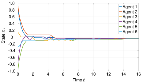
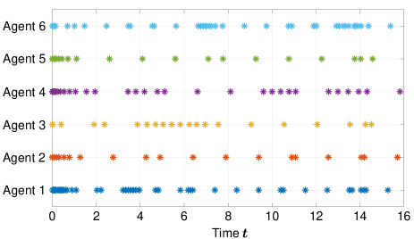
The state trajectory and the corresponding sampling times of each agent are shown in Figures 2 and 3, respectively, where the simulation time is 1616 and the time step is 10410^{-4}. From Figure 2, we see that the deviation of each state from the average state converges to zero. Figure 3 shows that sampling occurs frequently on the interval [0,1][0,1] but less frequently on the interval [1,16][1,16]. Agent 33 measures relative states more frequently on the interval [4,7][4,7] than on other intervals. This is because the state of agent 33 oscillates due to coarse quantization. Such oscillations can be observed also for other agents, e.g., agent 11 on the interval [3,4][3,4]. Moreover, we find in Figure 2 that the states of agents 22 and 55 do not change on the intervals [2,4][2,4] and [2,7][2,7], respectively. This is also caused by coarse quantization. In fact, the quantized values of their relative state measurements are zero on these intervals. However, the proposed algorithm ensures that the quantization errors exponentially converge to zero, and hence the multi-agent system achieves asymptotic consensus.

Refer to caption
Figure 2. State trajectories.
Refer to caption
Figure 3. Sampling times.

7. Conclusion

We have proposed a joint design method of a finite-level dynamic quantizer and a self-triggering mechanism for asymptotic consensus by relative state information. The inter-event times are bounded from below by a strictly positive constant, and the sampling times can be computed efficiently by using the Lambert WW-function. The quantizer has been designed so that saturation is avoided and quantization errors exponentially converge to zero. The new semi-norm introduced for the consensus analysis is constructed based on the maximum norm, and the matrix exponential of the negative Laplacian matrix has the semi-contractivity property with respect to the semi-norm. Future work will focus on extending the proposed method to the case of directed graphs and agents with high-order dynamics.

8. Acknowledgments

This work was supported by JSPS KAKENHI Grant Number JP20K14362.

References

  • [1] Fax, J.A., Murray, R.M.: ‘Information flow and cooperative control of vehicle formations’, IEEE Trans Automat Control, 2004, 49, pp. 1465–1476
  • [2] Olfati.Saber, R., Shamma, J.S. ‘Consensus filters for sensor networks and distributed sensor fusion’. In: Proc. 44th IEEE Conf. Decis. Control, 2005. pp.  6698–6703
  • [3] Olfati-Saber, R., Murray, R.M.: ‘Consensus problems in networks of agents with switching topology and time-delays’, IEEE Trans Automat Control, 2004, 49, pp. 1520–1533
  • [4] Olfati-Saber, R., Fax, J.A., Murray, R.M.: ‘Consensus and cooperation in networked multi-agent systems’, Proc IEEE, 2007, 95, pp. 215–233
  • [5] Chen, F., Ren, W.: ‘On the control of multi-agent systems: A survey’, Found Trends Syst Control, 2019, 6, pp. 339–499
  • [6] Årzén, K.E. ‘A simple event-based PID controller’. In: Proc. 14th IFAC World Congress. vol. 18, 1999. pp.  423–428
  • [7] Tabuada, P.: ‘Event-triggered real-time scheduling of stabilizing control tasks’, IEEE Trans Automat Control, 2007, 52, pp. 1680–1685
  • [8] Heemels, W.P.M.H., Sandee, J., van den Bosch, P.: ‘Analysis of event-driven controllers for linear systems’, Int J Control, 2008, 81, pp. 571–590
  • [9] Velasco, M., Fuertes, J., Marti, P. ‘The self triggered task model for real-time control systems’. In: Proc. 24th IEEE Real-Time Syst. Symp, 2003. pp.  67–70
  • [10] Wang, X., Lemmon, M.D.: ‘Self-triggered feedback control systems with finite-gain 2\mathcal{L}_{2} stability’, IEEE Trans Automat Control, 2009, 54, pp. 452–467
  • [11] Anta, A., Tabuada, P.: ‘To sample or not to sample: Self-triggered control for nonlinear systems’, IEEE Trans Automat Control, 2010, 55, pp. 2030–2042
  • [12] Dimarogonas, D.V., Frazzoli, E., Johansson, K.H.: ‘Distributed event-triggered control for multi-agent systems’, IEEE Trans Automat Control, 2012, 57, pp. 1291–1297
  • [13] Seyboth, G.S., Dimarogonas, D.V., Johansson, K.H.: ‘Event-based broadcasting for multi-agent average consensus’, Automatica, 2013, 49, pp. 245–252
  • [14] Fan, Y., Liu, L., Feng, G., Wang, Y.: ‘Self-triggered consensus for multi-agent systems with Zeno-free triggers’, IEEE Trans Automat Control, 2015, 60, pp. 2779–2784
  • [15] Yi, X., Liu, K., Dimarogonas, D.V., Johansson, K.H.: ‘Dynamic event-triggered and self-triggered control for multi-agent systems’, IEEE Trans Automat Control, 2019, 64, pp. 3300–3307
  • [16] Liu, K., Ji, Z.: ‘Dynamic event-triggered consensus of general linear multi-agent systems with adaptive strategy’, IEEE Trans Circuits Syst II, Exp Briefs, 2022, 69, pp. 3440–3444
  • [17] Ding, L., Han, Q.L., Ge, X., Zhang, X.M.: ‘An overview of recent advances in event-triggered consensus of multiagent systems’, IEEE Trans Cybern, 2018, 48, pp. 1110–1123
  • [18] Nowzari, C., Garcia, E., Cortés, J.: ‘Event-triggered communication and control of networked systems for multi-agent consensus’, Automatica, 2019, 105, pp. 1–27
  • [19] Dimarogonas, D.V., Johansson, K.H.: ‘Stability analysis for multi-agent systems using the incidence matrix: Quantized communication and formation control’, Automatica, 2010, 46, pp. 695–700
  • [20] Ceragioli, F., De Persis, C., Frasca, P.: ‘Discontinuities and hysteresis in quantized average consensus’, Automatica, 2011, 47, pp. 1916–1928
  • [21] Liu, S., Li, T., Xie, L., Fu, M., Zhang, J.F.: ‘Continuous-time and sampled-data-based average consensus with logarithmic quantizers’, Automatica, 2013, 49, pp. 3329–3336
  • [22] Guo, M., Dimarogonas, D.V.: ‘Consensus with quantized relative state measurements’, Automatica, 2013, 49, pp. 2531–2537
  • [23] Wu, Y., Wang, L.: ‘Average consensus of continuous-time multi-agent systems with quantized communication’, Int J Robust Nonlinear Control, 2014, 24, pp. 3345–3371
  • [24] Li, J., Ho, D.W.C., Li, J.: ‘Adaptive consensus of multi-agent systems under quantized measurements via the edge Laplacian’, Automatica, 2018, 92, pp. 217–224
  • [25] Xu, T., Duan, Z., Sun, Z., Chen, G.: ‘A unified control method for consensus with various quantizers’, Automatica, 2022, 136, Art. no. 110090
  • [26] Garcia, E., Cao, Y., Yu, H., Antsaklis, P., Casbeer, D.: ‘Decentralised event-triggered cooperative control with limited communication’, Int J Control, 2013, 86, pp. 1479–1488
  • [27] Zhang, Z., Zhang, L., Hao, F., Wang, L.: ‘Distributed event-triggered consensus for multi-agent systems with quantisation’, Int J Control, 2015, 88, pp. 1112–1122
  • [28] Zhang, Z., Zhang, L., Hao, F., Wang, L.: ‘Periodic event-triggered consensus with quantization’, IEEE Trans Circuits Syst II, Expr Briefs, 2016, 63, pp. 406–410
  • [29] Yi, X., Wei, J., Johansson, K.H. ‘Self-triggered control for multi-agent systems with quantized communication or sensing’. In: Proc. 55th IEEE Conf. Decis. Control, 2016. pp.  2227–2232
  • [30] Liu, Q., Qin, J., Yu, C. ‘Event-based multi-agent cooperative control with quantized relative state measurements’. In: Proc. 55th IEEE Conf. Decis. Control, 2016. pp.  2233–2239
  • [31] Wu, Z.G., Xu, Y., Pan, Y.J., Su, H., Tang, Y.: ‘Event-triggered control for consensus problem in multi-agent systems with quantized relative state measurements and external disturbance’, IEEE Trans Circuits Syst I, Reg Papers, 2018, 65, pp. 2232–2242
  • [32] Dai, M.Z., Xiao, F., Wei, B.: ‘Event-triggered and quantized self-triggered control for multi-agent systems based on relative state measurements’, J Frankl Inst, 2019, 356, pp. 3711–3732
  • [33] Li, K., Liu, Q., Zeng, Z.: ‘Quantized event-triggered communication based multi-agent system for distributed resource allocation optimization’, Inf Sci, 2021, 577, pp. 336–352
  • [34] Dai, M.Z., Fu, W., Zhao, D.J., Zhang, C. ‘Distributed self-triggered control with quantized edge state sampling and time delays’. In: Advances in Guidance, Navigation and Control. (Singapore: Springer, 2022. pp.  883–894
  • [35] Wang, F., Li, N., Yang, Y.: ‘Quantized-observer based consensus for fractional order multi-agent systems under distributed event-triggered mechanism’, Math Comput Simul, 2023, 204, pp. 679–694
  • [36] De Persis, C., Frasca, P.: ‘Robust self-triggered coordination with ternary controllers’, IEEE Trans Automat Control, 2013, 58, pp. 3024–3038
  • [37] Matsume, H., Wang, Y., Ishii, H.: ‘Resilient self/event-triggered consensus based on ternary control’, Nonlinear Anal: Hybrid Systems, 2021, 42, Art. no. 101091
  • [38] Golestani, F., Tavazoei, M.S.: ‘Event-based consensus control of Lipschitz nonlinea rmulti-agent systems with unknown input delay and quantization constraints’, Eur Phys J Spec Top, 2022, 231, pp. 3977–3985
  • [39] Carli, R., Bullo, F., Zampieri, S.: ‘Quantized average consensus via dynamic coding/decoding schemes’, Int J Robust Nonlinear Control, 2010, 20, pp. 156–175
  • [40] Li, T., Fu, M., Xie, L., Zhang, J.F.: ‘Distributed consensus with limited communication data rate’, IEEE Trans Automat Control, 2011, 56, pp. 279–292
  • [41] You, K., Xie, L.: ‘Network topology and communication data rate for consensusability of discrete-time multi-agent systems’, IEEE Trans Automat Control, 2011, 56, pp. 2262–2275
  • [42] Li, D., Liu, Q., Wang, X., Yin, Z.: ‘Quantized consensus over directed networks with switching topologies’, Syst Control Lett, 2014, 65, pp. 13–22
  • [43] Qiu, Z., Xie, L., Hong, Y.: ‘Quantized leaderless and leader-following consensus of high-order multi-agent systems with limited data rate’, IEEE Trans Automat Control, 2016, 61, pp. 2432–2447
  • [44] Ma, J., Ji, H., Sun, D., Feng, G.: ‘An approach to quantized consensus of continuous-time linear multi-agent systems’, Automatica, 2018, 91, pp. 98–104
  • [45] Chen, X., Liao, X., Gao, L., Yang, S., Wang, H., Li, H.: ‘Event-triggered consensus for multi-agent networks with switching topology under quantized communication’, Neurocomputing, 2017, 230, pp. 294–301
  • [46] Ma, J., Liu, L., Ji, H., Feng, G.: ‘Quantized consensus of multiagent systems by event-triggered control’, IEEE Trans Syst, Man, Cybern: Syst, 2018, 50, pp. 3231–3242
  • [47] Yu, P., Dimarogonas, D.V.: ‘Explicit computation of sampling period in periodic event-triggered multiagent control under limited data rate’, IEEE Trans Control Netw Syst, 2019, 6, pp. 1366–1378
  • [48] Lin, N., Ling, Q.: ‘Bit-rate conditions for the consensus of quantized multiagent systems based on event triggering’, IEEE Trans Cybern, 2022, 52, pp. 116–127
  • [49] Lin, N., Ling, Q.: ‘An event-triggered consensus protocol for quantized second-order multi-agent systems with network delay and process noise’, ISA Trans, 2022, 125, pp. 31–41
  • [50] Feng, S., Ishii, H.: ‘Dynamic quantized consensus of general linear multi-agent systems under denial-of-service attacks’, IEEE Trans Control Network Systems, 2022, 9, pp. 562–574
  • [51] Rikos, A.I., Hadjicostis, C.N.: ‘Event-triggered quantized average consensus via ratios of accumulated values’, IEEE Trans Automat Control, 2021, 66, pp. 1293–1300
  • [52] Rikos, A.I., Charalambous, T., Johansson, K.H., Hadjicostis, C.N.: ‘Distributed event-triggered algorithms for finite-time privacy-preserving quantized average consensus’, IEEE Trans Control Network Systems, 2023, 10, pp. 38–50
  • [53] Horaud, R., Hansard, M., Evangelidis, G., Ménier, C.: ‘An overview of depth cameras and range scanners based on time-of-flight technologies’, Mach Vis Appl, 2016, 27, pp. 1005–1020
  • [54] Spong, M.W., Hutchinson, S., Vidyasagar, M.: ‘Robot Modeling and Control’. 2nd ed. (Hoboken, NJ, USA: Wiley, 2020)
  • [55] Corless, R.M., Gonnet, G.H., Hare, D.E., Jeffrey, D.J., Knuth, D.E.: ‘On the Lambert WW function’, Adv Comput Math, 1996, 5, pp. 329–359
  • [56] Brockett, R.W., Liberzon, D.: ‘Quantized feedback stabilization of linear systems’, IEEE Trans Automat Control, 2000, 45, pp. 1279–1289
  • [57] Liberzon, D.: ‘Hybrid feedback stabilization of systems with quantized signals’, Automatica, 2003, 39, pp. 1543–1554
  • [58] Jafarpour, S., Cisneros.Velarde, P., Bullo, F.: ‘Weak and semi-contraction for network systems and diffusively coupled oscillators’, IEEE Trans Automat Control, 2022, 67, pp. 1285–1300
  • [59] De Pasquale, G., Smith, K.D., Bullo, F., Valcher, M.E. ‘Dual seminorms, ergodic coefficients and semicontraction theory’, to appear in IEEE Trans Automat Control 2023
  • [60] Pazy, A.: ‘Semigroups of Linear Operators and Applications to Partial Differential Equations’. (New York: Springer, 1983)

Appendix A: Proof of Proposition 4.10

Let 0<γλ2(L)0<\gamma\leq\lambda_{2}(L), and let Λ0\Lambda_{0}, Λ\Lambda, V0V_{0}, and VV be as in the proof of Lemma 4.1.

a) The inequality

22NΓ(γ)2-\frac{2}{N}\leq\Gamma_{\infty}(\gamma)

has already been proved in (26). It remains to show that

Γ(γ)N1.\Gamma_{\infty}(\gamma)\leq N-1.

Since V0N×NV_{0}\in\mathbb{R}^{N\times N} is orthogonal, we have V0N\|V_{0}\|_{\infty}\leq\sqrt{N}. Hence,

V=V01NN1N.\|V\|_{\infty}=\|V_{0}\|_{\infty}-\frac{1}{\sqrt{N}}\leq\sqrt{N}-\frac{1}{\sqrt{N}}.

Moreover, VV0=N\|V^{\top}\|_{\infty}\leq\|V_{0}^{\top}\|_{\infty}=\sqrt{N} and

Csupt0eγteΛt1.C\coloneqq\sup_{t\geq 0}\|e^{\gamma t}e^{-\Lambda t}\|_{\infty}\leq 1.

Therefore, the inequality (24) yields

Γ(γ)CVV(N1N)N=N1.\Gamma_{\infty}(\gamma)\leq C\|V\|_{\infty}\|V^{\top}\|_{\infty}\leq\left(\sqrt{N}-\frac{1}{\sqrt{N}}\right)\sqrt{N}=N-1.

b) Suppose that GG is a complete graph. Then

Λ0=diag(0,N,,N).\Lambda_{0}=\mathrm{diag}(0,\,N,\,\cdots,\,N).

If 0<γλ2(L)=N0<\gamma\leq\lambda_{2}(L)=N, then

eγt(eLt𝟏𝟏¯)eNt(eLt𝟏𝟏¯)\|e^{\gamma t}(e^{-Lt}-\mathbf{1}\bar{\mathbf{1}})\|_{\infty}\leq\|e^{Nt}(e^{-Lt}-\mathbf{1}\bar{\mathbf{1}})\|_{\infty}

for all t0t\geq 0. Hence, it suffices by a) to show that

(A1) supt0eNt(eLt𝟏𝟏¯)=22N.\sup_{t\geq 0}\|e^{Nt}(e^{-Lt}-\mathbf{1}\bar{\mathbf{1}})\|_{\infty}=2-\frac{2}{N}.

Using L=V0Λ0V0L=V_{0}\Lambda_{0}V_{0}^{\top} and

(A2) 𝟏𝟏¯=V0diag(1, 0,, 0)V0,\mathbf{1}\bar{\mathbf{1}}=V_{0}\,\mathrm{diag}(1,\,0,\,\cdots,\,0)\,V_{0}^{\top},

we obtain

eNt(eLt𝟏𝟏¯)\displaystyle e^{Nt}(e^{-Lt}-\mathbf{1}\bar{\mathbf{1}}) =V0(eNteΛ0tdiag(eNt, 0,, 0))V0\displaystyle=V_{0}\left(e^{Nt}e^{-\Lambda_{0}t}-\mathrm{diag}(e^{Nt},\,0,\,\cdots,\,0)\right)V_{0}^{\top}
=V0diag(0, 1,, 1)V0\displaystyle=V_{0}\,\mathrm{diag}(0,\,1,\,\cdots,\,1)\,V_{0}^{\top}

for all t0t\geq 0. Moreover, (A2) yields

V0diag(0, 1,, 1)V0\displaystyle V_{0}\,\mathrm{diag}(0,\,1,\,\cdots,\,1)\,V_{0}^{\top} =V0V0V0diag(1, 0,, 0)V0\displaystyle=V_{0}V_{0}^{\top}-V_{0}\,\mathrm{diag}(1,\,0,\,\cdots,\,0)\,V_{0}^{\top}
=I𝟏𝟏¯.\displaystyle=I-\mathbf{1}\bar{\mathbf{1}}.

Thus, (A1) holds by I𝟏𝟏¯=22/N\|I-\mathbf{1}\bar{\mathbf{1}}\|_{\infty}=2-2/N. ∎

Appendix B: Proof of Proposition 5.1

Define the function HH by

H(τ)τ+beτc,τ.H(\tau)\coloneqq\tau+be^{-\tau}-c,\quad\tau\in\mathbb{R}.

Then

τ+cbeτH(τ)0.-\tau+c\geq b{e^{-\tau}}\quad\Leftrightarrow\quad H(\tau)\leq 0.

Since

H(τ)=1beτ,H^{\prime}(\tau)=1-be^{-\tau},

it follows that H(τ)=0H^{\prime}(\tau)=0 holds at τ=logb\tau=\log b. From the assumption c<bc<b, we have H(0)>0H(0)>0. Therefore, there exists τ>0\tau>0 such that H(τ)0H(\tau)\leq 0 if and only if

(B1) logb>0andH(logb)0.\log b>0\quad\text{and}\quad H(\log b)\leq 0.

Since

H(logb)=logb+1c,H(\log b)=\log b+1-c,

it follows that (B1) is equivalent to

(B2) 1<be1+c.1<b\leq e^{-1+c}.

Hence,

inf{τ>0:τ+cbeωτ}=\inf\{\tau>0:-\tau+c\geq be^{-\omega\tau}\}=\infty

if (B2) does not hold.

The inequality τ+cbeτ-\tau+c\geq be^{-\tau} can be written as

(B3) (τc)eτcbec.(\tau-c)e^{\tau-c}\leq-be^{-c}.

Let W0W_{0} and W1W_{-1} be the primary and secondary branch of the Lambert WW-function, respectively. In other words, W0(y)W_{0}(y) and W1(y)W_{-1}(y) are the solutions x=x0[1,0)x=x_{0}\in[-1,0) and x=x1(,1]x=x_{-1}\in(-\infty,-1] of the equation xex=yxe^{x}=y for y[e1,0)y\in[-e^{-1},0), respectively. For each y[e1,0)y\in[-e^{-1},0),

(B4) xexyW1(y)xW0(y);xe^{x}\leq y\quad\Leftrightarrow\quad W_{-1}(y)\leq x\leq W_{0}(y);

see, e.g., [55].

Suppose that the condition (B2) holds. The expression (B3) and the equivalence (B4) show that τ+cbeτ-\tau+c\geq be^{-\tau} if and only if

W1(bec)+cτW0(bec)+c.W_{-1}(-be^{-c})+c\leq\tau\leq W_{0}(-be^{-c})+c.

Note that W1(bec)+cW_{-1}(-be^{-c})+c and W0(bec)+cW_{0}(-be^{-c})+c are the solutions of the equation H(τ)=0H(\tau)=0. Since H(0)>0H(0)>0, both solutions are positive. Thus,

inf{τ>0:τ+cbeτ}=W1(bec)+c\inf\{\tau>0:-\tau+c\geq be^{-\tau}\}=W_{-1}(-be^{-c})+c

is obtained. ∎