Semantic Recovery for Open-Set Domain Adaptation: Discover Unseen Categories in the Target Domain

Given the unlabeled target domain $\mathcal{D}_{t}=\{\mathbf{X}_{t}\}$ includes $N_{t}$ images belonging to $C_{t}$ categories drawn from the distribution $P_{t}$. We seek help from another auxiliary source domain $\mathcal{D}_{s}=\{\mathbf{X}_{s},\mathbf{Y}_{s},\mathbf{A_{s}}\}$ consisting of $N_{s}$ samples from $C_{s}$ categories and drawn from the distribution $P_{s}$, where $P_{s}\neq P_{t}$. In reality, $D_{s}$ cannot promise always cover the whole target domain label space, leading to the Open-Set problem where $C_{t}-C_{s}$ categories existing in the target domain but are unseen in the source domain. However, we are not satisfied with simply filtering out those unknown categories as most existing Open-Set domain adaptation solutions did, we would also like to explore target samples from unseen categories and discover them in a more meaningful way. Thus, we introduce the semantic description of those seen categories in the source domain, denoted as $\mathbf{A_{s}}\in\mathbb{R}^{C_{s}\times d_{a}}$, to learn enriched knowledge and representations for the visual images. The semantic descriptions describe the characteristics of each category, so they are class-level descriptions, instead of sample-level. In other words, for source samples belonging to the same category $c$, their semantic descriptions $\mathbf{a}_{s}^{i}=\mathbf{A}_{s}^{c}$, $\mathbf{a}_{s}^{i}\in\mathbb{R}^{d_{a}}$ are the same.

ZD: We should merge with the overall framework Moreover, we denote $\mathbf{X}_{s/t}\in\mathbb{R}^{N_{s/t}\times d_{x}}$ as the source/target features extracted by the pre-trained convolutional feature extractor, and $\mathbf{Y}_{s}\in\mathbb{R}^{N_{s}}$ denotes the source domain label set. It is noteworthy that, different from some generalized zero-shot learning tasks, we don’t expect the knowledge of the target domain unseen categories, no matter unseen classes numbers nor corresponding semantic descriptions. The goal of our work are recognizing the unlabeled target domain data into either seen categories as the source domain label space or the unseen set, and further explore the semantic descriptions of the all the target domain data especially for the samples from the target domain unseen set.

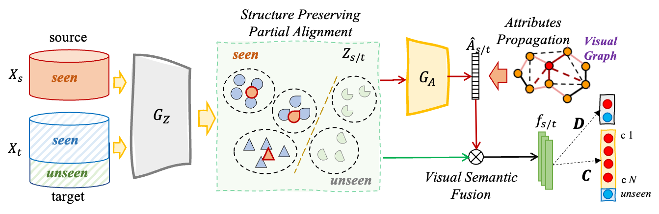
We illustrate the proposed framework of this paper as Fig. 1. Specifically, the framework consists of a Convolutional Neural Network $E(\cdot)$ as the feature extractor for both source and target domain, which extracts visual features $\mathbf{X}_{s/t}$ from raw images. $G_{Z}(\cdot)$ is a network mapping the source and target domain data into a shared feature space, from which the output is denoted as $\mathbf{z}_{s/t}^{i}=G_{Z}(\mathbf{x}_{s/t}^{i})$, $\mathbf{z}_{s/t}^{i}\in\mathbb{R}^{d_{z}}$. $G_{A}(\cdot)$ is used to mapping each sample from the visual feature space to the semantic feature space, and the predicted semantic description is denoted as $\hat{\mathbf{a}}_{s/t}^{i}=G_{A}(\mathbf{x}_{s/t}^{i})$ for each instance. $D(\cdot)$ is a binary classifier to recognize if the target domain data is from the seen categories or the unseen categories. $C(\cdot)$ is a classifier with output dimension as $C_{s}+1$, which can recognize the input sample is from which specific one of $C_{s}$ seen category or $1$ "unseen" set, and the predicted label is denoted as $\hat{y}_{s/t}^{i}$.

The most challenging and practical task we focus in this work is to reveal meaningful semantic descriptions for the target domain data no matter they are from the seen categories as the source domain or from the unseen categories only existing in the target domain. So we expect a projector $G_{A}(\cdot)$ to map the data from visual feature space into the semantic feature space.

However, because only the knowledge of labels and semantic descriptions from seen categories are available, both the source domain and the target domain High Confidence set $\mathcal{D}_{t}^{H}$ ignore the information and structure of those target samples from the unseen categories. Unfortunately, training the feature extractor $G_{Z}(\cdot)$ and the semantic projector $G_{A}(\cdot)$ only on $\mathcal{D}_{s}$ and $\mathcal{D}_{t}^{H}$ makes things worse because of overfitting to the seen categories, although we seek to explore the characteristics of data from unseen categories. So we explore the mechanism of semantic propagation to aggregate the visual features structural knowledge into the semantic description projection.

Specifically, for samples in a training batch drawn from the source or target domain, the adjacency matrix $A$ is calculated as $A_{ij}=\exp(-\frac{d_{ij}^{2}}{\sigma^{2}})$, where $A_{ij}=0,\forall i$, and $d_{ij}^{2}=\|\mathbf{z}^{i}-\mathbf{z}^{j}\|$ is the distance of two features $(\mathbf{z}^{i},\mathbf{z}^{j})$. $\sigma^{2}$ is a scaling factor and we accept $\sigma^{2}=Var(d_{ij}^{2})$ as [rodriguez2020embedding] to stabilize training. Then we calculate the Laplacian of the adjacency matrix $L=D^{-\frac{1}{2}}AD^{-\frac{1}{2}},\,\,D_{ii}=\sum_{j}A_{ij}$. Then, we have the semantic propagator matrix $\mathcal{W}=(I-\alpha L)^{-1}$ following the idea described in [zhou2004learning], and $\alpha\in\mattbb{R}$ is a scaling factor, and $I$ is the identity matrix. Finally, the semantic descriptions projected from the visual features are obtained as:

$$\hat{\mathbf{a}}_{s/t}^{i}=\sum_{j}\mathcal{W}_{ij}G_{A}(G_{Z}(\mathbf{x}_{s/t}^{i})).$$

(4)

After the semantic propagation, the projected semantic description $\mathbf{\tilde{a}}_{s/t}^{i}$ is refined as a weighted combination of the semantic representation of its neighbors guided by the visual features graph structure. Such strategy aggregates the visual features similarity graph knowledge into the semantic description projection, preventing the risks of overfitting to the seen categories during training, and has the effect of removing undesired noise from the visual and semantic features vectors [rodriguez2020embedding].

Then for each source domain sample $\mathbf{x}_{s}^{i}\in\mathbf{X}_{s}$, the ground-truth label $y_{s}^{i}$ is known, so does the semantic description $\mathbf{a}_{s}^{i}$, where $\mathbf{a}_{s}^{i}=\mathbf{A}_{s}^{y_{s}^{i}}$ is obtained from $\mathbf{A}_{s}$ by class label $y_{s}^{i}$. We construct the semantic projection loss on the source domain as:

$$\mathcal{L}_{s}^{A}=\frac{1}{N_{s}}\sum_{\mathbf{x}_{s}^{i}\in\mathcal{D}_{s}}L_{bce}(\hat{\mathbf{a}}_{s}^{i},\,\,\,\mathbf{a}_{s}^{i}),$$

(5)

where $L_{bce}(\cdot)$ is the binary cross-entropy loss. For each sample $\mathbf{x}_{s}^{i}$, each dimension value of the semantic description $\mathbf{a}_{s}^{i}\in\mathbb{R}^{d_{A}}$ represent one specific semantic characteristic, so each dimension of the $G_{A}(\cdot)$ output measures the predicted probability that the input sample has such specific characteristic.

For the target domain, although the ground-truth labels and semantic descriptions are not available, fortunately we have already obtained confident pseudo labels and pseudo semantic descriptions after the operations in Section 3.2.1. So for each target domain sample $\mathbf{x}_{t}^{i}\in\mathcal{D}_{t}^{H}$ from the High Confidence set, we accept its pseudo labels $\tilde{y}_{t}^{i}\in\mathbf{\tilde{Y}}_{t}^{H}$ to get the pseudo semantic descriptions $\mathbf{\tilde{a}}_{t}^{i}=\mathbf{A}_{s}^{\tilde{y}_{t}^{i}}$, as the samples in $\mathcal{D}_{t}^{H}$ all have pseudo labels from the seen categories shared between the source and target domain. Then similarly, we construct the semantic projection loss on the target domain as:

$$\mathcal{L}_{t}^{A}==\frac{1}{N_{t}^{H}}\sum_{\mathbf{x}_{t}^{i}\in\mathcal{D}_{t}^{H}}L_{bce}(\mathbf{\hat{a}}_{t}^{i},\,\,\,\mathbf{\tilde{a}}_{t}^{i}),$$

(6)

where $N_{t}^{H}$ is the number of samples in $\mathcal{D}_{t}^{H}$.

Combining them together, we have the semantic description projection objective as:

$${\underset{G_{Z},G_{A}}{\min}\mathcal{L}^{A}=\mathcal{L}_{s}^{A}+\mathcal{L}_{t}^{A}}$$

(7)

As the visual features and semantic descriptions explain the data from different perspectives in various modalities, we explore the joint distribution of both visual and semantic descriptions for each data simultaneously. Inspired by [long2017conditional], for each sample $\mathbf{z}^{i}=G_{Z}(\mathbf{x}^{i})$, we convey the semantic discriminative information $\mathbf{a}^{i}$ into the visual features by construct the joint representation as:

$$\mathbf{f}^{i}=\mathbf{z}^{i}\oplus\mathbf{a}^{i},$$

(8)

where $\oplus$ is the concatenation operation to combine the visual and semantic features $\mathbf{z}^{i}$ and $\mathbf{a}^{i}$ to construct a joint distribution $\mathbf{f}^{i}$, which will be used to do the classification optimization and cross-domain alignment.

It is noteworthy that we have already introduced several different semantic descriptions for each sample from different subsets, thus we will obtain various joint representations for the data as:

$$\left\{\begin{matrix}[l]\,\,\mathcal{F}_{s}^{i}\quad=\{\mathbf{\bar{f}}_{s}^{i},\mathbf{\hat{f}}_{s}^{i}\},&\mathbf{x}_{s}^{i}\in\mathcal{D}_{s}\\ \mathcal{F}_{t}^{H(j)}=\{\mathbf{\tilde{f}}_{t}^{j},\mathbf{\hat{f}}_{t}^{j}\},&\mathbf{x}_{t}^{j}\in\mathcal{D}_{t}^{H}\\ \mathcal{F}_{t}^{L(k)}=\{\mathbf{\hat{f}}_{t}^{k}\},&\mathbf{x}_{t}^{k}\in\mathcal{D}_{t}^{L}\end{matrix}\right.,$$

(9)

pecifically, for the source domain data $\mathbf{x}_{s}^{i}\in\mathcal{D}_{s}$, we can construct $\mathbf{\bar{f}}_{s}^{i}=\mathbf{z}_{s}^{i}\oplus\mathbf{a}_{s}^{i}$ with the ground-truth semantic description $(\mathbf{a}_{s}^{i})$, and $\mathbf{\hat{f}}_{s}^{i}=\mathbf{z}_{s}^{i}\oplus\mathbf{\hat{a}}_{s}^{i}$ is with the projected semantic description $\mathbf{\hat{a}}_{s}^{i}=G_{A}(\mathbf{z}_{s}^{i})$. Similarly, for the target domain High Confidence data $\mathbf{x}_{t}^{j}\in\mathcal{D}_{t}^{H}$, pseudo semantic feature $(\mathbf{\tilde{a}}_{t}^{j})$ can be obtained by pseudo label $\mathbf{\tilde{y}}_{t}^{j}$, together with the semantic representation prediction $\mathbf{\hat{a}}_{t}^{j}=G_{A}(\mathbf{z}_{t}^{j})$, we can construct two kind of joint representation as $\mathbf{\tilde{f}}_{t}^{j}=\mathbf{x}_{t}^{j}\oplus\mathbf{\tilde{a}}_{t}^{j}$, and $\mathbf{\hat{f}}_{t}^{j}=\mathbf{z}_{t}^{j}\oplus\mathbf{\hat{a}}_{t}^{j}$. Finally, for all data $\mathbf{x}_{t}^{k}\in\mathcal{D}_{t}^{L}$, the only semantic description we have is the prediction $(\mathbf{\hat{a}}_{t}^{k})$ projected by $G_{A}(\mathbf{z}_{t}^{k})$, and we can construct the joint representation as $\mathbf{\hat{f}}_{t}^{k}=\mathbf{z}_{t}^{k}\oplus\mathbf{\hat{a}}_{s/t}^{k}$. All the joint representations $\mathcal{F}_{s},\mathcal{F}_{t}^{H},\mathcal{F}_{t}^{L}$ are input to the classifier $C(\cdot)$ and $D(\cdot)$ to optimize the framework.

Domain adaptation assumes that with the help of labeled source domain data, we can train a model to transferable to the unlabeled target domain data. A lot of existing domain adaptation works have proven the reasonableness and effectiveness of such strategy. So maintaining the ability of the model on the source domain data is crucial for transferring the model to the target domain tasks. For each source domain sample $\mathbf{x}_{s}^{i}\in$, the ground-truth label $y_{s}^{i}$ is known. We construct the classification loss on the source domain as:

$$\mathcal{L}_{s}^{C}=\frac{1}{N_{s}}\sum_{\mathbf{x}_{s}^{i}\in\mathcal{D}_{s}}\sum_{\mathbf{f}_{s}^{i}\in\mathcal{F}_{s}^{i}}L_{ce}(C(\mathbf{f}_{s}^{i}),y_{s}^{i}),$$

(10)

where $L_{ce}(\cdot)$ is the cross-entropy loss.

Moreover, we have already obtained confident pseudo labels for the target domain data, which are also accepted to optimize the model to the target domain. It is noteworthy that $C(\cdot)$ is an extended classifier recognizing the input instance into $C_{s}+1$ classes, which includes $C_{s}$ seen categories shared across domains plus the additional "unseen" class. Specifically, for samples from the High Confidence set $\mathcal{D}_{t}^{H}$, the model is optimized to recognize them as the corresponding pseudo labels in $\mathbf{\tilde{Y}}_{t}^{H}$. For the samples from the Low Confidence set $\mathcal{D}_{t}^{L}$, the classifier $C(\cdot)$ recognize them as the "unseen" class. Thus we have the loss term on the target domain as:

	$\displaystyle\mathcal{L}_{t}^{C}$	$\displaystyle=\frac{1}{N_{t}^{H}}\sum_{\mathbf{x}_{t}^{i}\in\mathcal{D}_{t}^{H}}\sum_{\mathbf{f}_{t}^{i}\in\mathcal{F}_{t}^{H(i)}}L_{ce}(C(\mathbf{f}_{t}^{i}),\,\,\phi(\tilde{y}_{t}^{i}))$		(11)
		$\displaystyle+\frac{1}{N_{t}^{L}}\sum_{\mathbf{x}_{t}^{i}\in\mathcal{D}_{t}^{L}}\sum_{\mathbf{f}_{t}^{i}\in\mathcal{F}_{t}^{L(i)}}L_{ce}(C(\mathbf{f}_{t}^{i}),\,\,\phi(\tilde{y}_{t}^{i})),$

where $\phi(\tilde{y}_{t}^{i})=\tilde{y}_{t}^{i}$ if $\mathbf{x}_{t}^{i}\in\mathcal{D}_{t}^{H}$, $\phi(\tilde{y}_{t}^{i})=C_{s}+1$ if $\mathbf{x}_{t}^{i}\in\mathcal{D}_{t}^{L}$, and $N_{t}^{H/L}$ denotes the number of samples in $\mathcal{D}_{t}^{H/L}$. Then we have our classification supervision objective on both source and target domain as:

$$\underset{G_{Z},G_{A},C}{min}\mathcal{L}^{C}=\mathcal{L}_{s}^{C}+\mathcal{L}_{t}^{C}$$

(12)

To more accurately recognize the target domain data into seen and unseen subsets, we further train a binary classifier $D(\cdot)$ to finely separate the seen and unseen classes. With the help of the joint representations of the target domain as input and the pseudo labels and pseudo semantic descriptions available, the fine-grained binary classifier $D(\cdot)$ can be optimized by:

	$\displaystyle\mathcal{L}_{t}^{D}$	$\displaystyle=\frac{1}{N_{t}^{H}}\sum_{\mathbf{x}_{t}^{i}\in\mathcal{D}_{t}^{H}}\sum_{\mathbf{f}_{t}^{i}\in\mathcal{F}_{t}^{H(i)}}L_{bce}(C(\mathbf{f}_{t}^{i}),\,\,\psi(\tilde{y}_{t}^{i}))$		(13)
		$\displaystyle+\frac{1}{N_{t}^{L}}\sum_{\mathbf{x}_{t}^{i}\in\mathcal{D}_{t}^{L}}\sum_{\mathbf{f}_{t}^{i}\in\mathcal{F}_{t}^{L(i)}}L_{bce}(C(\mathbf{f}_{t}^{i}),\,\,\psi(\tilde{y}_{t}^{i})),$

in which $\psi(\tilde{y}_{t}^{i})$ indicate if the target sample $\mathbf{x}_{t}^{i}$ if from the seen categories ($\mathbf{x}_{t}^{i}\in\mathcal{D}_{t}^{H},\psi(\tilde{y}_{t}^{i})=0$), or from the unseen categories ($\mathbf{x}_{t}^{i}\in\mathcal{D}_{t}^{L},\psi(\tilde{y}_{t}^{i})=1$).

A lot of previous domain adaptation efforts focus on exploring a domain invariant feature space across domains. However, due to the mismatch of the source and target domains label space in our task, simply matching the feature distribution across domains becomes destructive. Moreover, the distribution structural information has been proven important for the label space mismatch tasks like conventional open-set domain adaptation [pan2020exploring]. Considering our goal of uncovering the unseen categories in the target domain, preserving the structural knowledge of the target domain data becomes even more crucial. Thanks to the refined prototypes $\mathcal{R}_{\mathbf{x}}$ and the pseudo labels $\mathbf{\tilde{Y}}_{t}$ for target domain data we already obtained in Section 3.2.1, we can get the prototype $\mathcal{R}_{\mathbf{z}}$ on the embedding features $\mathbf{z}_{t}$ with the help of pseudo labels $\mathbf{\tilde{Y}}_{t}$ in the similar way. Specifically, for each pseudo label $c$, the corresponding prototype can be calculated as $\mathcal{R}_{\mathbf{z}}^{c}=\mathbb{E}_{\mathbf{x}\in\mathcal{D}_{t}}\mathbf{z}_{t}^{i}\cdot\mathbb{I}_{\tilde{y}_{t}^{i}=c}$. The prototypes of the target domain features describe the structural graph knowledge in the target domain, thus we propose the loss function to enforce the target domain data closer to their corresponding prototypes based on the pseudo labels as:

	$\displaystyle\mathcal{L}_{t}^{R}=$	$\displaystyle\frac{1}{N_{t}}\sum_{\mathbf{x}_{t}^{i}\in\mathcal{D}_{t}}(d(\mathbf{z}_{t}^{i},\mathcal{R}_{\mathbf{z}}^{c})\cdot\mathbb{I}_{\tilde{y}_{t}^{i}=c}$		(14)
		$\displaystyle-\frac{1}{C_{s}+K-1}\sum d(\mathbf{z}_{t}^{i},\mathcal{R}_{\mathbf{z}}^{c}{}^{\prime})\cdot\mathbb{I}_{\tilde{y}_{t}^{i}\neq c^{\prime}}),$

where $\mathcal{R}_{\mathbf{z}}^{c/c^{\prime}}$ denotes the prototype with label $c/c^{\prime}$, $C_{s}+K=|\mathcal{R_{\mathbf{z}}}|$ is the total number of prototypes in $\mathcal{R}_{\mathbf{z}}$, and $d(\cdot)$ is the distance measurement between two features. Such loss function pushes the embedding feature of the target sample $\mathbf{z}_{t}^{i}=G_{Z}(\mathbf{x}_{t}^{i})$ close to the corresponding prototype $\mathcal{R}_{\mathbf{z}}^{c}$ with pseudo label $c=\tilde{y}_{t}^{i}$, while further away from other prototypes $\mathcal{R}_{\mathbf{z}}^{c^{\prime}}$ where $c^{\prime}\neq\tilde{y}_{t}^{i}$.

Moreover, for the source domain data, we seek to map the source domain data into the target domain feature space, to preserve the target domain distribution structure, instead of mapping both source and target domain into a shared feature space as such strategy may break the original structural knowledge in the target domain. Then we propose the loss function on the source domain as:

	$\displaystyle\mathcal{L}_{s}^{R}=$	$\displaystyle\frac{1}{N_{s}}\sum_{\mathbf{x}_{s}^{i}\in\mathcal{D}_{s}}(d(\mathbf{z}_{s}^{i},\mathcal{R}_{\mathbf{z}}^{c})\cdot\mathbb{I}_{y_{s}^{i}=c}$		(15)
		$\displaystyle-\frac{1}{C_{s}+K-1}\sum d(\mathbf{z}_{s}^{i},\mathcal{R}_{\mathbf{z}}^{c}{}^{\prime})\cdot\mathbb{I}_{y_{s}^{i}\neq c^{\prime}}).$

It is noteworthy that, these two loss functions simultaneously achieve the cross-domain partial alignment and enhancing the discriminative characteristics in the embedding feature space while preserving the target domain data structure. Thus we get our structure preserving partial cross-domain alignment loss as:

$$\underset{G_{Z}}{min}\mathcal{L}^{R}=\mathcal{L}_{s}^{R}+\mathcal{L}_{t}^{R}$$

(16)

Overall, we propose our final optimization objective as:

$${\underset{G_{Z},G_{A},C,D}{min}}\mathcal{L}^{A}+\mathcal{L}^{C}+\mathcal{L}_{t}^{D}+\mathcal{L}^{R}$$

(17)

We evaluate our method in two ways, open-set and semantic recovery. For open-set is same as the conventional open-set domain adaptation works did, recognizing the whole target domain data into the seen categories shared between the source and target domain, or 1 unseen category. We report the results of the classifier $C(\cdot)$ with the performance only on the seen categories (OS^∗), unseen categories (OS^⋄), and overall accuracy (OS) on the whole target data [panareda2017open]. For the semantic recovery task, we evaluate the predicted semantic description projected by $G_{A}(\cdot)$ by applying the prototypical classification with the ground-truth semantic attributes from all classes to get the classification accuracy on the whole target domain label space. We report the performances on the seen categories and unseen categories as $U$ and $S$, respectively, and calculate the harmonic mean $H$, defined as $H=(2\times S\times U)/(S+U)$, to evaluate the performance on both seen and unseen categories. It is noteworthy that all results we reported are the average of class-wise top-1 accuracy, to eliminate the influence of imbalance of data distribution across classes. Furthermore, we will show the explored semantic attributes for some target samples from the unseen categories to intuitively evaluate the performance of discovering unseen classes only exist in the target domain.

PGL (2020 ICML) [luo2020progressive]

TIM (2020 CVPR) [kundu2020towards]

AOD (2019 ICCV) [feng2019attract]

SAT (2019 CVPR) [liu2019separate]

USBP (2018 ECCV) [saito2018open]

ANMC (2020 IEEE TMM) [shermin2020adversarial]

(ZSL)

(GZSL)

TF-CLSGAN (2020 ECCV) [narayan2020latent]

FFT (2019 ICCV) [zhu2019learning]

CADA-VAE (2019 CVPR) [schonfeld2019generalized]

GDAN (2019 CVPR) [Huang_2019_CVPR]

LisGAN (2019 CVPR) [Li19Leveraging]

Cycle-WGAN (2018 ECCV) [felix2018multi]

(Transductive Generalized Zero-Shot Learning)

We use the binary attributes of AwA2 from corresponding classes as the semantic descriptions. ImageNet pre-trained ResNet-50 is accepted as the backbone, and we take the output before the last fully connected layer as the features $\mathbf{X}_{s/t}$ [deng2009imagenet, he2016deep]. $G_{Z}(\cdot)$ is two-layer fully connected neural networks with hidden layer output dimension as 1024, and the output feature dimension is 512. $C(\cdot)$ and $D(\cdot)$ are both two-layer fully connected layer neural network classifier with hidden layer output dimension as 256, and the output dimension of $C(\cdot)$ is $C_{s}+1$, while $D(\cdot)$ output as two classes. $G_{A}(\cdot)$ is two-layer neural networks with hidden layer output dimension as 256 followed by ReLU activation, and the final output dimension is the same as the semantic attributes dimension followed by Sigmoid function. We accept the cosine distance for the prototypical classification, while all other distances used in the paper are Euclidean distance.