Semi-implicit Integration and Data-Driven Model Order Reduction in Structural Dynamics with Hysteresis
Indian Institute of Technology Kanpur
To appear in ASME Journal of Computational and Nonlinear Dynamics )
Abstract
Structural damping is often empirically rate-independent wherein the dissipative part of the stress depends on the history of deformation but not its rate of change. Hysteresis models are popular for rate-independent dissipation; and a popular hysteresis model is the Bouc-Wen model. If such hysteretic dissipation is incorporated in a refined finite element model, then the model involves the usual structural dynamics equations along with nonlinear nonsmooth ordinary differential equations for a large number of internal hysteretic states at Gauss points used within the virtual work calculation. For such systems, numerical integration is difficult due to both the distributed non-analytic nonlinearity of hysteresis as well as large natural frequencies in the finite element model. Here we offer two contributions. First, we present a simple semi-implicit integration approach where the structural part is handled implicitly based on the work of Piché, while the hysteretic part is handled explicitly. A cantilever beam example is solved in detail using high mesh refinement. Convergence is good for lower damping and a smoother hysteresis loop. For a less smooth hysteresis loop and/or higher damping, convergence is noted to be roughly linear on average. Encouragingly, the time step needed for stability is much larger than the time period of the highest natural frequency of the structural model. Subsequently, data from several simulations conducted using the above semi-implicit method are used to construct reduced order models of the system, where the structural dynamics is projected onto a few modes and the number of hysteretic states is reduced significantly as well. Convergence studies of error against the number of retained hysteretic states show very good results.
1 Introduction
Modelling of damping in materials is a classical problem in structural dynamics, and not a fully solved one. The high dimensionality of structural finite element models combine with the non-analyticity of physically realistic damping models to produce numerical challenges in dynamic simulation. This paper makes two contributions in this area. The first contribution, which concerns simple but effective numerical integration, leads to the second contribution, which is in data-driven model order reduction.
Although the linear viscous damping model is simple and convenient, it is not always correct. For many materials subjected to periodic loading, the internal dissipation per cycle is frequency-independent [1]. In the linear viscous damping model the dissipation per cycle is proportional to frequency. Hysteretic dissipation, which is a rate-independent [2] mechanism, is preferred by many structural dynamicists because it is more realistic. However, hysteresis involves nonanalytic behavior with slope changes at every reversal of loading direction. Numerical integration for structural dynamics with hysteretic damping needs more care than with linear viscous damping. The difficulty grows greatly with finite element models wherein mesh refinement leads to high structural frequencies requiring tiny time steps; and wherein the nonanalytic hysteretic damping is finely resolved in space as well.
In this paper we first consider time integration of the vibration response for beams111Our approach extends directly to frames modeled using beam elements. The approach may eventually be generalized to two or three dimensional elements. with distributed hysteretic damping, and then consider model order reduction by projecting the dynamics onto a few vibration modes. Model order reduction is not trivial in this case because the distributed hysteresis needs to be projected onto lower dimensions as well. Initial numerical solutions of the full system, using a semi-implicit integration scheme developed in this paper, are subsequently used to construct lower order models with hysteretic damping. Our newly introduced integration scheme provides an efficient way to generate the data needed for the second part of the paper. In principle, other integration methods could be used as well, but they are either more complicated or more slow.
1.1 Explicit, implicit, and semi-implicit integration
A key idea in numerical integration of ordinary differential equations (ODEs) is outlined here for a general reader.
We consider ODE systems written in first order form, , where is a state vector and is time. In single-step methods, which we consider in this paper, we march forward in time using some algorithm equivalent to
| (1) |
The specific form of above is derived from the form of and depends on the integration algorithm. The actual evaluation of may involve one or multiple stages, but that is irrelevant: the method is single-step in time. For smooth systems, is guided by the first few terms in Taylor expansions of various quantities about points of interest in the current time step. In such cases, as , the error in the computed solution goes to zero like for some . If , the convergence is called superlinear. If , the convergence is called quadratic. Values of are easily possible for smooth systems with moderate numbers of variables: see, e.g., the well known Runge-Kutta methods [3]. Unfortunately, for large structural systems, for the asymptotic rate to hold, may need to be impractically small. For example, the highest natural frequency of a refined finite element (FE) model for a structure may be, say, Hz. This structure may be forced at, say, 10 Hz. A numerical integration algorithm that requires time steps that resolve the highest frequency in the structure, i.e., time steps much smaller than seconds in this example, is impractical. A high order of convergence that requires time steps smaller than is of little use. We seek accurate results with time steps much smaller than the forcing period, but much larger than the time period of the highest natural frequency of the structure, e.g., or seconds. To develop such practically useful algorithms, we must consider the stability of the numerical solution for larger values of , i.e., , say.
Now consider the nature of . If does not depend explicitly on , the algorithm is explicit. Otherwise it is implicit. For nonlinear systems, is a nonlinear function of its -arguments. Then each implicit integration step requires iterative solution for . For linear dynamics, with linear in its -arguments, the can be moved over to the left hand side and integration proceeds without iteration, although usually with matrix inversion. The algorithm is still called implicit in such cases: implicitness and iteration are not the same. An algorithm can be neither fully implicit nor fully explicit, and we will present one such algorithm in detail.
1.2 Contribution of this paper
We present a semi-implicit approach that can be used for high dimensional finite element models with distributed hysteresis. For simplicity, we adopt the popular Bouc-Wen model [4, 5, 6] as our damping mechanism. After presenting and validating our numerical integration method, we present a way to obtain useful lower order models for the structure, starting from a refined FE model. A key issue is that the refined or full FE model computes hysteretic variables at a large number of Gauss points in the structure, and a smaller subset needs to be used for the model order reduction to be practical.
Thus, our contribution is twofold. First, we present a simple semi-implicit algorithm for a structural FE model with distributed hysteresis and demonstrate its convergence and utility. Second, we use this algorithm to compute some responses of the structure and use those responses to construct accurate lower order models with reduced numbers of both vibration modes and hysteretic variables. These lower order models can be used later for quick simulations under similar initial conditions or loading.
1.3 Representative literature review
We begin with a review of some numerical integration methods that are available in popular software or research papers.
Structural systems with Bouc-Wen hysteresis continue to be studied in research papers using algorithms that are not as efficient as the one we will present below. For example, as recently as 2019, Vaiana et al. [14] considered a lumped-parameter model and used an explicit time integration method from Chang’s family [15]. That method requires tiny time steps: the authors used one hundredth of the time period of the highest structural mode. Such small time steps are impractical for refined FE models. Our algorithm allows much larger time steps. Thus, in the area of FE models with distributed hysteresis, our paper makes a useful contribution.
Next, we acknowledge that the commercial finite element software Abaqus [7] allows users to specify complex material responses and also to choose between explicit and implicit numerical integration options. For many nonlinear and nonsmooth dynamic problems, explicit integration needs to be used in Abaqus. As outlined above, implicit or semi-implicit algorithms can be useful for somewhat simpler material modeling and in-house FE codes.
Considering general purpose software for numerical work, many analysts dealing with hysteresis may begin with Matlab [10]. Matlab’s built in function ode15s is designed for stiff systems but not specifically for systems with hysteresis. We have found that ode15s can handle ODEs from FE models with a modest number of elements and with hysteresis, but it struggles with higher numbers of elements because its adaptive time steps become too small. In this paper we will use ode15s to obtain numerically accurate solutions for systems of moderate size. Results obtained from our own algorithm will then be validated against ode15s results. Subsequently, for larger systems, our algorithm will continue to work although ode15s freezes and/or crashes.
For those programming their own integration routines in structural dynamics, the well known Newmark method [11] from 1959 remains popular (see, e.g., [9, 8]), although it cannot guarantee stability and may require tiny time steps as noted in, e.g., [12]. In that paper [12] of 1977, Hilber, Hughes and Taylor modified the Newmark method and showed unconditional stability for linear structural problems. However, their method (known as HHT-) can show spurious oscillations of higher modes even without hysteretic damping (see, e.g., Fig. 7 of the paper by Piché [31], which we will take up below).
An appreciation of the issues faced for full three-dimensional (3D) simulation with hysteretic damping can be gained, e.g., from the work of Triantafyllou and Koumousis [13]. Their formulation is actually based on plasticity in 3D; they compare their solutions with those from Abaqus; and they include dynamics through the Newmark algorithm. Their algorithm is rather advanced for a typical analyst to implement quickly. Note that our present application is easier than theirs because we have only one-dimensional Bouc-Wen hysteresis. Additionally, our primary application here is in model order reduction. And so we develop for our current use a numerical integration approach that is simpler than that in [13].
Finally, readers interested in hybrid simulations (with an experimental structure in the loop) may see, e.g., Mosqueda and Ahmadizadeh [16, 17] who used a modified version of the HHT- for calculating the seismic response of a multi-degree-of-freedom structure. Purely simulation-based studies such as the present one can hopefully provide theoretical inputs into planning for such hybrid simulations in future work.
We close this section with a brief discussion of model oder reduction. While there are very many papers on the topic, we make special note of the condensation approaches of Guyan [18] and Irons [19], wherein finding normal modes of the full system was avoided. With growth in computational power, system eigenvectors become more easily available, and direct modal projection has become common. For a recent discussion of this and related methods, see [20]. We will use straightforward modal projection for our displacement degrees of freedom. However, we will also have a large number of internal hysteretic state variables. We will present a sequential approach to selecting a subset of these hysteretic variables, using an algorithm which is related closely to a method called “QR with column pivoting” in [21]. Minor differences from [21] here are that we work with rows and not columns, and our data matrix is not rank deficient: we separately impose a termination criterion.
Note that modal reduction, without the added complication of hysteretic damping, is well known. For example, Stringer et al.[22, 23] successfully applied modal reduction to rotor systems, including ones with gyroscopic effects. Other recent examples in dynamics and vibrations can be seen in [24, 25]. Proper Orthogonal Decomposition (POD) [26] based reduced order models are often used in fluid mechanics: a representative sample may be found in [27, 28, 29, 30].
1.4 Overview of our approach
We will begin by adopting an existing implicit scheme for linear structural dynamics without hysteresis that is both simple and significantly superior to both the Newmark and HHT- methods. Our adopted scheme, due to Piché [31], is an L-stable method from the Rosenbrock family (see [32] and references therein) which is stable, implicit without iteration for linear structures, and second order accurate. For smooth nonlinear systems of the form
Piché suggests a one-time linearization of at the start of each time step. We will not use that linearization step because hysteresis is nonsmooth.
Here we extend Piché’s formulation to include hysteretic damping in the otherwise-linear structural dynamics. In our method the stiffness and inertia terms are integrated implicitly (without iteration, being linear) and the nonsmooth hysteresis is monitored at Gauss points [33] and treated with explicit time-integration. Thus, overall, our method is semi-implicit. Our proposed approach, when applied to a refined FE model of an Euler-Bernoulli beam with distributed Bouc-Wen hysteretic damping, is easy to implement and can be dramatically faster than Matlab’s ode15s. In fact, it continues to work well beyond refinement levels where ode15s stops working.
We emphasize that ode15s is not really designed for such systems. We use it here because it has adaptive step sizing and error estimation: when it does work, it can be highly accurate. For this reason, to examine the performance of our algorithm for modest numbers of elements, we will use results obtained from ode15s with a tight error tolerance. With higher number of elements, ode15s fails to run because the time steps required become too small.
Having shown the utility of our proposed semi-implicit integration algorithm, we will turn to our second contribution of this paper, namely model order reduction. Such Reduced Order Models (ROMs) can save much computational effort. In the physical system, if only a few lower modes are excited, the displacement vector can be approximated as a time-varying linear combination of those modes only. A remaining issue here is that the number of Gauss points used for the hysteresis can be reduced too, and that is where we offer an additional contribution.
In recent work related to ours, for an Euler-Bernoulli beam with hysteretic dissipation, Maity et al. [33] used the first few undamped analytically obtained modes to approximate the solution and performed the virtual work integration using a few Gauss points chosen over the full domain. However, they used a different hysteresis model motivated by distributed microcracks. Furthermore, in our finite element model, virtual work integrations are performed over individual elements and not the whole domain. The number of Gauss points in the finite element model increases with mesh refinement. When we project the response onto a few modes, we can explicitly reduce the number of Gauss points retained as well, and a practical method of doing so is one of the contributions of this paper.
2 Governing equations and Finite Element formulation
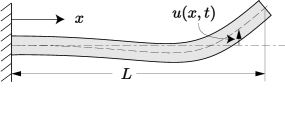
The governing equation of the deflection of a cantilever beam (shown in Fig. (1)) with a dissipative bending moment is
| (2) |
where the beam’s material density, cross section and flexural rigidity are , and respectively. The parameter is the strength of hysteretic dissipation. The hysteretic damping variable is defined at each -location along the beam length, is governed pointwise by the Bouc-Wen model, and is driven pointwise by the local curvature
in the governing equation
| (3) |
where the Bouc-Wen model parameters satisfy
| (4) |
The parameters in Eq. (4) and the hysteretic variable are dimensionless. The dissipation strength parameter has units of Nm (i.e., units of moments).
The FE model involves beam elements for displacement variables, virtual work calculations for the hysteretic moment through domain integrals based on Gauss points within each element, and ODE solution in time. We use the Galerkin method wherein we look for an admissible solution so that the residual,
| (5) |
is orthogonal to basis functions for the space of . Mathematically,
| (6) |
where
is the inner product between two functions, is the spatial domain over which the basis functions are defined, and is the basis function.
2.1 Element matrices and virtual work integrals
The elemental stiffness and inertia matrices are routine and given in many textbooks: each beam element has two nodes, and each node has one translation and one rotation. The hysteresis variable is a scalar quantity distributed in space. However, it enters the discretized equations through integrals, and so values only need to be known at Gauss points within each element. The evolution of at the Gauss points is computed using Eq. (3), and is thus driven by displacement variables. Some further details are given in appendix A.
2.2 Global equations
After assembly we obtain a system of equations of the form
| (7a) | |||
| where , , and . The hysteresis rate equations are given by | |||
| (7b) | |||
where and the different symbols mean the following:
-
1.
is a column vector of nodal displacements and rotations for beam elements, with for a cantilever beam,
-
2.
and are mass and stiffness matrices of size ,
-
3.
is a column vector of length from Gauss points per element,
-
4.
and denote elementwise multiplication and exponentiation,
-
5.
is a matrix of weights used to convert values into virtual work integrals,
-
6.
is a column vector of curvatures at the Gauss points,
-
7.
maps nodal displacements and rotations to curvatures at the Gauss points, and
-
8.
incorporates applied forces.
In Eq. (7a) above we can include viscous damping by adding , for some suitable , on the left hand side. As this paper focuses on hysteretic damping, we have taken
3 Time integration
We will develop a semi-implicit method adapted from Piché’s [31] work. Equation (7a) has a structural part (stiffness and inertia) and a hysteresis part. The structural part is integrated implicitly (section 3.1) and the hysteresis part marches in time, following an explicit algorithm which takes care of the nonsmooth slope changes due to zero-crossing of the time derivative of the curvature (section 3.2). In section 4, our semi-implicit algorithm will be used to generate a large amount of data which will be used to construct reduced order models.
3.1 Implicit integration for the structural part
Piché’s algorithm uses a numerical parameter which is written as for compact presentation. The symbol should not be confused for Euler’s constant. We now proceed as follows. This subsection presents implicit integration for the structural part alone: the hysteretic variable vector is not integrated in an implicit step: this compromise simplifies the algorithm greatly.
-
1.
Define
(The is dropped if linear viscous damping is no included.)
-
2.
Define
-
3.
Define (first stage)
-
4.
Define (second stage)
and
-
5.
Finally
-
6.
Define
Note that the assignment of to above is tentative at this stage; if there is a sign change, we will make a correction, as discussed in the next subsection.
3.2 Explicit integration for the hysteretic part
Due to the nonanalyticity of hysteresis models, we integrate the hysteresis part using an explicit step. There are slope changes in the hysteretic response whenever at any Gauss point crosses zero in time. We will accommodate the sign change of within an explicit time step in a second sub-step, after first taking a time step assuming that there is no sign change. Since each depends on only, accounting for zero crossings can be done individually for individual Gauss points and after such a preliminary step.
We first check elementwise and identify the entries of and that have same sign, and construct sub-vectors and out of those entries. The corresponding elements from the vector are used to construct a sub-vector . Here the subscript “” stands for “unchanged”. These elements can be used in a simple predictor-corrector step for improved accuracy as follows.
and
| (8) |
Next, we address the remaining entries of and , those that have crossed zero and flipped sign. We construct sub-vectors and out of them, where the “” subscript stands for “flipped”. The corresponding elements from the vector are used to construct sub-vector . Using linear interpolation to approximate the zero-crossing instants within the time step, we use
We define
and
which is consistent with Eq. (8) because at the end of the sub-step. Next we complete the step using
and
where is a vector of the same dimensions as and with all elements equal to . Finally, having the incremented values at all locations, those with signs unchanged and those with signs flipped, we use
We clarify that the explicit integration of the hysteretic variables, as outlined in this subsection, is a compromise adopted to avoid difficulties due to the nonanalyticity of the hysteresis model. Continuing to integrate the inertia and stiffness parts explicitly will still allow us to use usefully large steps, as will be seen in section 5.
Having the numerical integration algorithm in place, however, we must now turn to the second contribution of this paper, namely model order reduction.
4 Model order reduction
For reduced order modeling, we must reduce both the number of active vibration modes as well as the number of Gauss points used to compute the hysteretic dissipation. Of these two, the first is routine.
4.1 Reduction in the number of vibration modes
The undamped normal modes and natural frequencies are given by the eigenvalue problem
| (9) |
for eigenvector-eigenvalue pairs . In a finely meshed FE model, is large. In such cases, we may compute only the first several such pairs using standard built-in iterative routines in software packages.
The dimensional displacement vector is now approximated as a linear combination of modes. To this end, we construct a matrix with the first eigenvectors as columns so that
| (10) |
where , and where the elements of are called modal coordinates. Substituting Eq. (10) in Eq. (7a) and pre-multiplying with the transposed matrix , we obtain
| (11) |
obtaining equations of the form
| (12a) | |||
| (12b) |
In the above, due to orthogonality of the normal modes, the matrices and are diagonal. Also, is an approximation of the original because we have projected onto a few vibration modes, but it still has the same number of elements as and requires numerical integration of the same number of nonsmooth hysteresis equations. A reduction in the number of hysteretic variables is necessary.
4.2 Reduction in the number of hysteretic variables
The system still has a large number () of hysteretic damping variables. These are arranged in the elements of in Eq. (7a). Selecting a smaller set of basis vectors and projecting the dynamics of the evolving onto those has analytical difficulties. Here we adopt a data-driven approach to select a submatrix of , say
| (13) |
The indices must now be chosen form the set , along with a matrix , such that
| (14) |
Working with that reduced set of hysteretic variables, we will be able use a reduced set of driving local curvatures
| (15) |
a submatrix of . In other words, we will work with a subset of the original large number of Gauss points used to compute virtual work integrals for the hysteretic dissipation. In our proposed data-driven approach, selection of the indices is the only significant issue. The matrix can then be found by a simple matrix calculation.
However, for implementing our approach, we must first generate a sufficiently large amount of data using numerical integration of the full equations with representative initial conditions and/or forcing.
These initial conditions are randomly generated as follows. The hysteretic states are uniformly distributed random numbers in the interval (0, 0.1). For the displacement and rotation degrees of freedom, the initial conditions have nonzero values along only the first three modes. These initial conditions, in all cases, are scaled to make the tip displacement to be 2 cm. The three modal coordinate values are three randomly chosen, positive, independent and identically distributed numbers, subsequently rearranged so that the first mode had the largest displacement and the third mode had the smallest displacement. The initial values of the velocity degrees of freedom are taken to be zero. In applications, users who have other preferred criteria for choosing representative initial conditions can freely use them with no consequences for the rest of the algorithm.
Having selected initial conditions, we must simulate the system by integrating the equations forward in time. To that end, we use the semi-implicit integration method presented in section (3).
The data generation process is relatively slow, but once it is done and the reduced order model is constructed, we can use it for many subsequent quicker calculations. Beyond its academic interest, our approach is practically useful in situations where the reduced order model will be used repeatedly after it is developed.
It is perhaps not strictly necessary to place both of our contributions within one paper, but in our implementation the second part relies heavily on the first part; moreover, the second part is a relatively small and simple application of an efficient method to generate the needed data.
4.2.1 Selecting a subset of hysteretic variables
For data generation, we numerically integrate the full system, over some time interval with points in time. This process is carried out times with different random representative initial conditions as described above. The integration duration is chosen as 1 second, which gives several cycles of oscillation of the lowest mode along with some significant decay in oscillation amplitude. For each such solution with a random initial condition, upon arranging the variables’ solutions side by side in columns, a matrix of size is generated. This matrix is divided by its Frobenius norm, i.e., the square root of the sum of squares of all elements. We stack such normalized matrices, one from each simulation, side by side to form a bigger matrix of size . Clearly, the dimension of the row-space of is at most , because that is the total number of rows. Identification of a useful subset of hysteretic variables is equivalent to identifying a useful subset of the rows of . Therefore the problem we face now is that of selecting rows of which contain a high level of independent information.
Selecting a finite subset of the rows of is a combinatorial optimization problem. For example, if we start with and want to select a subset of size, say, 100, then the total number of subsets possible is extremely large and only a modest number of them can realistically be checked. Sometimes low-rank approximations to data matrices can be obtained using the proper orthogonal decomposition (POD) [26], but that technique is not useful here because it does not select a subset of rows.
Here, for a simple practical solution, we use a greedy algorithm that is closely related to a use of the QR decomposition (rank deficient least squares solutions) discussed in [21]. Although it is not guaranteed to give the best solution, we will see that it does give a reasonably good solution.
-
1.
Of all the rows of , we first select the one with the largest 2-norm and set it aside; we also record its index (or row number), which we call . We scale the row to unit norm, calculate its inner products with the rest of the rows of , and subtract from them their respective components along the row direction, yielding a modified .
-
2.
Next, of all the so far unselected rows of the modified , we select the one with the largest 2-norm; we record its row number in the original , and call it . We normalize the row and subtract its component along the still-remaining rows. This yields a further modified .
-
3.
To clarify, we now have two indices selected ( and ); and rows of remaining in contention, where for each of these remaining rows their components along the already-selected rows have been removed.
-
4.
Proceeding as above, we select a third row (largest 2-norm among the rows). We record its row number (call it ), normalize the row, and remove its component from the remaining rows.
-
5.
We proceed like this for as many rows as we wish to include in the reduced order model. A termination criterion based on the norm of the remaining part can be used if we wish.
-
6.
In the end, we are interested only in the selected indices . What remains of the matrix is discarded.
-
7.
In the above description, we could have removed the rows from after selecting them. That would leave a remaining matrix with progressively fewer rows as the calculation proceeded. That alternative algorithm is outlined below for ease of understanding.
For intuitive understanding through a simple example, we now describe the above procedure using small hypothetical numbers. The data matrix has, say, rows (for simplicity). Let the 4th row have the largest 2-norm. Let this row be denoted by . We select the fourth row, remove it from the data matrix, and obtain a new matrix with 9 rows. We divide by its 2-norm to obtain a unit vector, say . We take the inner product of with each of the 9 remaining rows, and subtract from these rows their components along . The new data matrix has rows that are all orthogonal to . Let the 5th row of this remaining matrix have the largest 2-norm. We must remember that this index, namely 5, was actually 6 in the original 10-row data matrix. With that caveat, we are back to the second line of this paragraph, only with 9 rows instead of 10. We proceed in this way for as many rows as we wish to select, or until the 2-norms of the remining rows become small enough.
4.2.2 Finding matrix P
With the indices chosen, a submatrix is assembled using the rows ofthe original (and not the reduced) . We now solve the straightforward least squares problem,
| (16) |
where denotes the Frobenius norm. The above problem, upon taking matrix transposes, is routine in, e.g., Matlab. The final reduced order model becomes
| (17a) | |||
| (17b) |
where is a submatrix of constructed by retaining the rows of the latter.
Equations 17a and 17b are equivalent to a dimensional system of first order equations ( modes and hysteretic variables). Note that the right hand side of Eq. (17a) may seem like it has a large number of elements, but in practice for many problems, external forcing is restricted to a few locations or can be reduced to a few effective locations (e.g., if the forces acting at several nodes maintain fixed proportions to each other). We do not investigate this aspect of size reduction because we have so far not made simplifying assumptions about . When the forcing is zero, of course, the right hand side is zero.
We now turn to the results obtained using, first, our integration routine; and then our approach for developing reduced order models.
5 Results
Our main aim is accurate simulation of hysteretic dissipation, which is most easily seen in the unforced decaying response of the structure. So we will first consider some unforced transient responses of the structure to examine both stability and numerical accuracy of our semi-implicit integration algorithm. Subsequently we will present reduced order models and show their efficacy compared to the full model.
In the results from direct numerical integration using our proposed semi-implicit algorithm, we will check for three things: (i) the theoretically expected power law decay for small amplitude vibrations, (ii) the absence of instabilities arising from higher modes, and (iii) overall accuracy.
For error calculations with low dimensional systems, i.e., when the number of elements in the FE model is small, we will use Matlab’s ode15s for comparison with both the absolute and relative error tolerances set to ; this is because ode15s has built-in adaptive step sizing and is accurate when it works. For high dimensional systems ode15s does not work and we will use the proposed semi-implicit algorithm itself with a very small step size for error estimates.
We now select some parameter values to be used in the simulation.
5.1 Choice of parameter values
We consider a cantilever beam with Young’s modulus GPa and density ; of length and square cross section of . This yields a flexural rigidity and mass per unit length .
For many metals, 0.2% strain is near the border of elastic behavior. For the beam parameters above, if the beam is statically deflected under a single transverse tip load, then 0.2% strain at the fixed end of the beam corresponds to a tip deflection of 6 cm, which is taken as a reasonable upper bound for the vibration amplitudes to be considered in our simulations below.
Next, we consider the hysteretic damping itself. The index in the Bouc-Wen model is primarily taken to be 0.5 for reasons explained a little later. A larger value is considered in subsection 5.4, and only in subsection 5.4, to clarify an issue in convergence. The parameters and are somewhat arbitrary; we have found that the values and yield hysteresis loops of reasonable shape. It remains to choose the Bouc-Wen parameter .
It is known that for small amplitude oscillations, the Bouc-Wen dissipation follows a power law. An estimate for the upper limit of forcing amplitude in the Bouc-Wen model, below which the power law should hold, is given in [35] as
| (18) |
Choosing to correspond to the abovementioned 0.2% strain at the fixed end, in turn corresponding to a static free-end deflection of 6 cm for the above beam, we find from Eq. (18) that
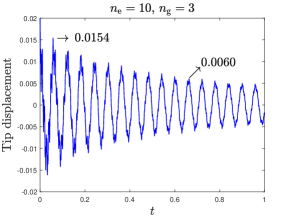
Only one physical model parameter remains to be chosen, namely . To choose this parameter value, we note that the amplitude decay in free vibrations with Bouc-Wen hysteretic dissipation is not exponential. Thus, the idea of percentage of damping is only approximately applicable. Upon looking at the reduction in amplitude after a certain number of oscillations (say ), an equivalent “percentage damping” can be approximated using the formula
| (19) |
Metal structures often have 1-2 % damping [34]. We will choose values of the hysteretic dissipation (recall Eq. (2)) to obtain . Numerical trial and error show that
is a suitable value (see figure 3).
5.2 Semi-implicit integration: stability and accuracy
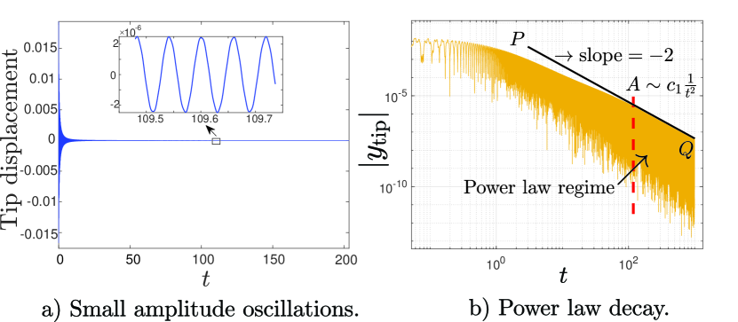
Before we examine the performance of our proposed semi-implicit integration method, we will verify that the FE model indeed displays power law damping at small amplitudes, as predicted by theoretical analyses of the Bouc-Wen model.
The small amplitude dissipation per cycle of the Bouc-Wen model is proportional to amplitude to the power [35]. Since the energy in the oscillation is proportional to amplitude squared, we should eventually observe small amplitude oscillations in the most weakly damped mode with amplitude obeying
whence for
| (20) |
For the Bouc-Wen model, letting produces hysteresis loops of parallelogram-like shape, and so we prefer somewhat larger values of ; however, to have a significant decay rate even at small amplitudes, we prefer somewhat smaller values of . As a tradeoff, we have chosen . We expect an eventual decay of vibration amplitudes like .
For our beam model, with 10 elements and 3 Gauss points per element, and with our semi-implicit numerical integration algorithm222Matlab’s ode15s struggles with such long simulations on a small desktop computer; our algorithm works quickly., the computed tip displacement asymptotically displays the expected power law decay rate, as seen on linear axes in Fig. (4a) and more clearly in the logarithmic plot of Fig. (4b). The frequency of the residual oscillation is close to the first undamped natural frequency of the beam. Higher modes are not seen in the long-term power law decay regime.
Having checked the asymptotic power law decay rate, we next ensure that the semi-implicit algorithm does not produce spurious oscillations in higher modes within the computed solution. This issue is important because, with increasing mesh refinement in the FE model, very high frequencies are unavoidable. While those high frequency modes exist in principle, their response should be small if any external excitation is at low frequencies and initial conditions involve only the lower modes. To examine this aspect, we denote the time period of the highest mode present in the structural model by . As the number of elements increases, decreases, as indicated in Fig. (5a).
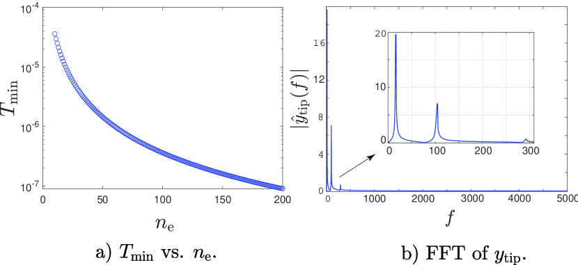
We now use our semi-implicit method to simulate an FE model with 100 elements and with nonzero initial conditions along only the first 3 modes. In the computed solution, we expect to see frequency content corresponding to the first three modes only. Figure 5b indeed shows only three peaks. Spurious responses of the higher modes are not excited. Note that this simulation was done with a time step of , which is more than 275 times larger than the time period of the highest mode for , which is (see Fig. (5a)). It is the implicit part of the code that allows stable numerical integration with such a large step size.
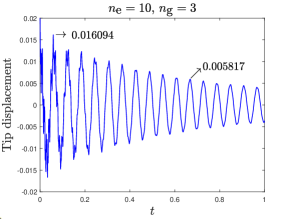
Having checked that spurious oscillations in very high modes are not excited, it remains to check that accurate results are obtained with time steps which are sufficiently small compared to the highest mode of interest. To this end, the convergence of the solution with decreasing is depicted in Fig. (6). For the beam modeled using 10 elements, the first five natural frequencies are
Numerical simulation results using our semi-implicit algorithm are shown in Fig. (6) for , and . The overall solution is plotted on the left, and a small portion is shown enlarged on the right. Only 10 elements were used for this simulation to allow use of Matlab’s ode15s, which has adaptive step sizing and allows error tolerance to be specified (here we used ). It is seen in the right subplot that although all three solutions from the semi-implicit method are stable, the one with does not do very well in terms of accuracy; the one with is reasonably close and may be useful for practical purposes; and the one with is indistinguishable at plotting accuracy from the ode15s solution. The match between our semi-implicit integration with and Matlab’s ode15s with error tolerances set to indicates that both these solutions are highly accurate.
5.3 Order of convergence
Using simulations with relatively few elements and over relatively short times, we can compare the results obtained from our semi-implicit method (SIM) with ode15s, and examine convergence as is made smaller.
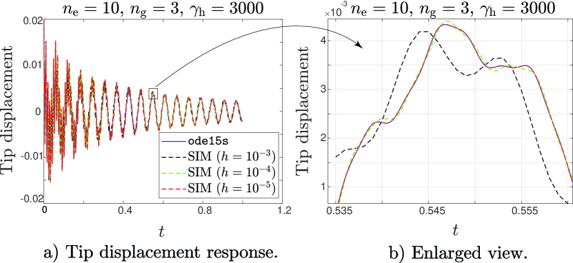
Figure 6 shows the tip response for an FE model with 10 elements for different time step sizes and compares them with the ode15s solution. Here we will use two different error measures.
5.3.1 RMS error
We choose a fairly large number () of points evenly spaced in time, and for each we calculate the response at those instants of time. The overall time interval was chosen to be [0,1]. Clearly, can be successively halved in a sequence of simulations to ensure that the solution is always computed at exactly the time instants of interest (along with other intermediate points).
We define our RMS error measure as
| (21) |
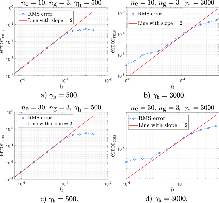
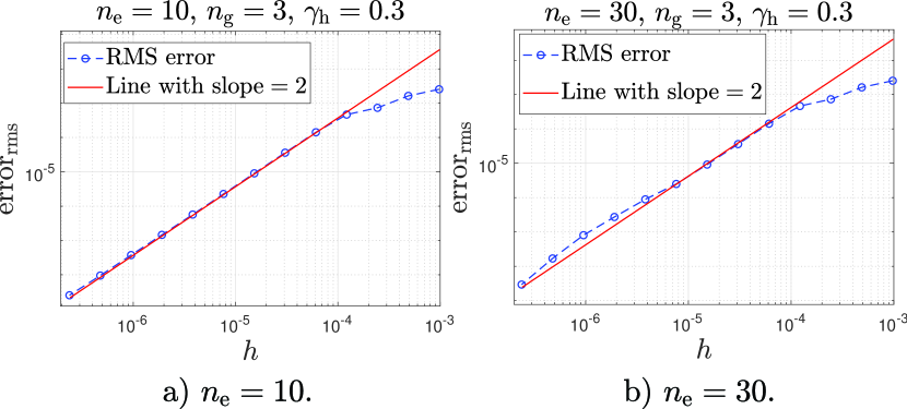
In the above, when the number of elements is modest (e.g., ), we use the highly accurate solution obtained from ode15s as the “accurate” one. With larger numbers of elements, ode15s cannot be used for validation. Having seen the overall accuracy of the semi-implicit method (SIM) with fewer elements when compared with ode15s, we use the SIM solution with extremely small time steps as the “accurate” one for error estimation with larger number of elements (e.g., ). Results are shown in Fig. (7). It is seen that for relatively smaller values of , a significant regime of approximately quadratic convergence is obtained (Fig. (7a,7c)). It means that for lightly damped structures the performance of the semi-implicit algorithm is excellent. For larger values of , however, the convergence plot is more complicated, and there is no significant regime of quadratic convergence (Fig. (7b,7d)). This is because the damping model is strongly non-analytic, and strong damping makes the role of that non-analyticity stronger. However, over a significant regime and in an average sense, it appears that the convergence is superlinear (i.e., the average slope exceeds unity in a loglog plot), and so the integration algorithm still performs well. A larger value will be considered in subsection 5.4.
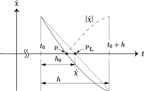
The role of nonanalyticity in the Bouc-Wen model, and the way in which it is handled in our semi-implicit algorithm, are worth emphasizing. See Fig. (8).
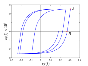
In the figure, point A shows a discontinuous slope change due to the sign change of the driving term, . This point is handled with an explicit attempt to locate the instant of change in direction, with one integration step taken on each side of that instant. Point B indicates a sign change in . Our proposed algorithm does not separately identify sign changes of within one time step, in the interest of simplicity. Due to nonanalyticity at both points A and B, integration errors increase when the nonsmoothness dominates (high and/or small ). A larger value will be considered in subsection 5.4.
5.3.2 Error at a fixed instant of time
We now consider the absolute value of error at some fixed instant of time ,
| (22) |
Here, we use .
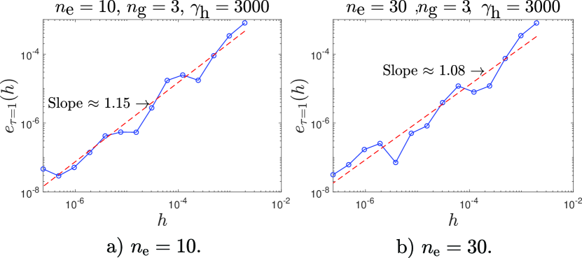
Straight line fits on loglog plots of versus in Fig. (9a,9b) show average slopes that slightly exceed unity. While these slopes are not rigorously proved to exceed unity, the overall convergence rate of the integration algorithm may be considered roughly linear (on average) over a sizeable range of step sizes. It is emphasized that these error computations are done in a regime where (i) Matlab’s ode15s does not work at all, (ii) explicit methods are unstable unless extremely small time steps are used, (iii) properly implicit algorithms are both complex and not guaranteed to converge, and (iv) in the Bouc-Wen model is relatively small. Considering these four difficulties, the semi-implicit method (SIM) proposed in this paper may be said to be simple, effective, and accurate.
5.4 Larger
Everywhere in this paper except for this single subsection, we have used . In this subsection only, we consider . Due to the greater smoothness of the hysteresis loop near the point B of Fig. (8), we expect better convergence for this higher value of .
Some parameter choices must be made again. Using the yield criteria used in section 5.1, for , we find we now require
Subsequently, we find an approximate equivalent damping ratio for . It is interesting to note that with the change in and for the physical behavior regime of interest, and have individually changed a lot but their product has varied only slightly (195 Nm for about 1.6% damping in the case, and 183 Nm for about 1.5% damping in the case).
The decay of tip response amplitude (Fig. (10)) for these parameters (with ) looks similar to the case studied in the rest of this paper (, with attention to Fig. (3)).
The main point to be noted in this subsection is that with , , , and all other parameters the same as before, we do indeed observe superior convergence over a significant range of step sizes: see Fig. (11) for FE models with 10 and 30 elements, and compare with Fig. (7). For the case with 10 elements, the convergence is essentially quadratic. With 30 elements the convergence is slightly slower than quadratic, but much faster than linear. Note that these estimates are from numerics only: analytical estimates are not available.
As mentioned above some of the difficulty with accurate integration of hysteretically damped structures comes from the zero crossings of the hysteretic variable itself. In this paper, for simplicity, we have avoided special treatment of these zero crossings. However, the results of this subsection show that the effect of these zero crossings is milder if is larger.
We now turn to using results obtained from this semi-implicit integration method to develop data-driven lower order models of the hysteretically damped structure.
5.5 Reduced order models
In our beam system, we have 2 degrees of freedom per node (one displacement and one rotation). Let the total number of differential equations being solved, in first order form, be called . If there are elements, we have first order differential equations. In a reduced order model with modes and Gauss points, we have first order differential equations. Although the size of the problem is reduced significantly in this way, the accuracy can be acceptable.
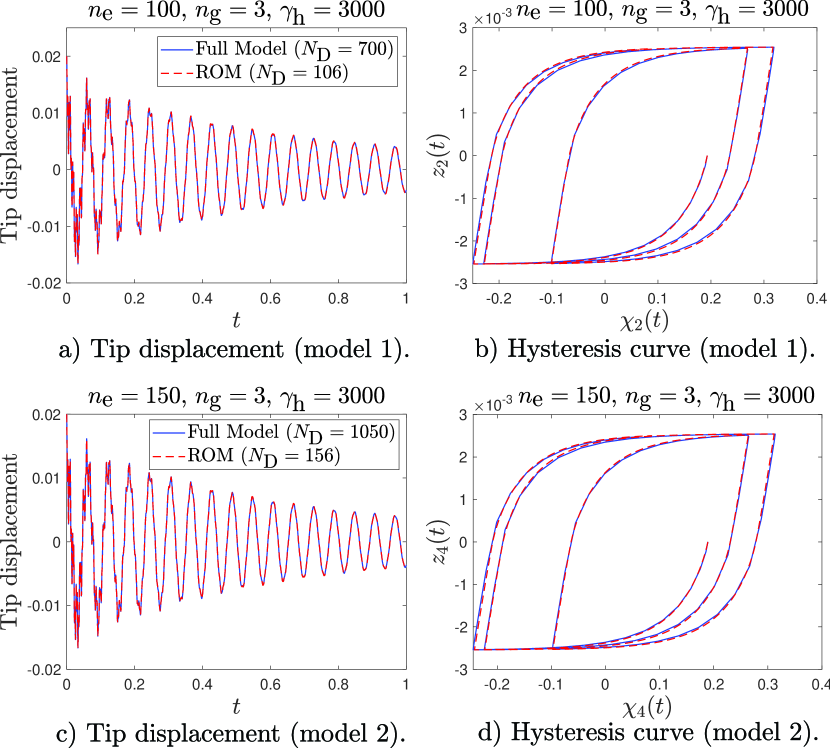
For demonstration, we consider two FE models of a cantilever beam, with hysteresis, as follows:
-
(i)
100 elements with 3 Gauss points each ().
-
(ii)
150 elements with 3 Gauss points each ().
For each of the two systems above, the datasets used for selecting the subset of hysteretic states (or Gauss points) were generated by solving the full systems 60 times each for the time interval 0 to 1 with random initial conditions and time step , exciting only the first 3 modes (). Data from each of these 60 solutions were retained at 1000 equispaced points in time (; recall subsection 4.2.1).
All reduced order model (ROM) results below are for retained modes. Further, the number of hysteresis Gauss points is denoted by . Results for are shown in Fig. (12a,12c).
We now quantitatively assess the accuracy of the ROMs. To this end, we write and for the ROM and full model outputs respectively. We then compute the error measure
| (23) |
for different values of and for an integration time interval (with ).
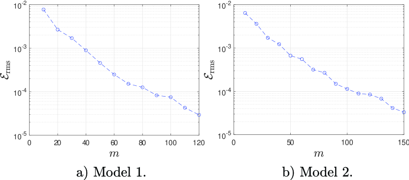
The variation of with , for both models, is shown in Fig. (13). This error measure is not normalized. If we wish to normalize it, then we should use the quantity obtained when we set identically to zero: that quantity is 0.006 for both models. Thus, reasonable accuracy is obtained for , and good accuracy (about 1% error) is obtained only for . These numbers refer to a specific case with random initial conditions; however, Fig. (13) is representative for other, similar, initial conditions (details omitted).
Finally, we report on run times needed on a modest laptop computer with the different levels of modeling described above. A representative initial conditions similar to the above was selected. The simulation duration was chosen to be 1 second, and the time step taken was seconds. The following results were obtained after averaging run times for 4 runs each. (i) The full simulation with our algorithm took an average of 27.22 seconds per run. (ii) After projecting on to 3 normal modes but retaining all 450 hysteretic states, each run took an average of 1.3 seconds. (iii) Finally, with 3 normal modes and hysteretic states reduced from 450 to 150, each run took an average of 0.84 seconds. Note that we could save further run time by taking larger time steps after model order reduction and/or retaining even fewer hsyteretic states.
6 Conclusions
Structural damping is nonlinear and, empirically, dominated by rate-independent mechanisms. Hysteresis models are therefore suitable, but present numerical difficulties when used in large finite element models. Fully implicit numerical integration of such highly refined FE models presents difficulties with convergence in addition to algorithmic complexities. With this view, we have proposed simpler but effective approaches, in two stages, to simulations of such structural dynamics. The first stage consists of a semi-implicit integration routine that is relatively simple to implement, and appears to give linear convergence or better. Moreover, the time steps required for stability can be much larger than the time period of the highest mode in the FE model. Subsequently, we have used the results from that semi-implicit integration to develop data-driven reduced order models for subsequent rapid case studies or other simulations.
Thus, our contribution is twofold: first, we present a simple and practical numerical integration method that can be easily implemented; second, we use the results from that integration algorithm to further reduce the size of the model.
Although we have worked exclusively with a cantilever beam in this paper, our approach can be directly extended to frames that can be modeled using beam elements. We hope that future work will also examine ways in which the present approach can be extended to genuinely two- or three-dimensional structures. While we have not worked such cases out yet, we are hopeful that the issues addressed in the present paper will help to tackle such higher-dimensional problems.
Acknowledgements
Aditya Sabale helped BG with the initial finite element formulation for beams. AC thanks the Department of Science and Technology, Government of India, for earlier support on a project to study hysteretic damping; this work arose from a continued interest in that topic.
Appendix A Finite element formulation details
| (25) |
where , . The generalised force corresponding to the coordinate is given by
Letting ,
| (26) |
where , . The are the Gauss integration points and their corresponding weights.
The dynamics of hysteretic dissipating moments at the Gauss points within an element are governed by the equations
| (27) |
where is the curvature at the Gauss point.
| (28) |
where
| (29) |
References
- [1] Kimball, A. L., and Lovell, D. E., 1927, Internal friction in solids. Physical Review, 30(6): 948.
- [2] Muravskii, G. B., 2004, On frequency independent damping. Journal of Sound and Vibration, 274(3-5): 653-668.
- [3] Chapra, S. C., and Canale, R. P., 2011, Numerical methods for engineers, Vol. 1221, Mcgraw-hill, New York.
- [4] Bouc, R., 1967, Forced vibrations of mechanical systems with hysteresis. Proc. of the Fourth Conference on Nonlinear Oscillations, Prague.
- [5] Wen, Yi-Kwei., 1976, Method for random vibration of hysteretic systems. Journal of the Engineering Mechanics Division, 102(2): 249-263.
- [6] Visintin, A., 2013, Differential models of hysteresis. Springer Science and Business Media, Vol. 111.
- [7] Abaqus, G., 2011, Abaqus 6.11. Dassault Systemes Simulia Corporation, Providence, RI, USA.
- [8] Lee, T. Y., Chung, K. J., and Chang, H., 2017, A new implicit dynamic finite element analysis procedure with damping included. Engineering Structures, 147: 530-544.
- [9] Bathe, K. J., 2007, Conserving energy and momentum in nonlinear dynamics: a simple implicit time integration scheme. Computers & Structures, 85(7-8): 437-445.
- [10] MATLAB, 2010, version 7.10.0 (R2010a). The MathWorks Inc, Natick, Massachusetts.
- [11] Newmark, N. M., 1959, A method of computation for structural dynamics. Journal of the Engineering Mechanics Division, 85(3): 67-94.
- [12] Hilber, H. M., Hughes, T. J., and Taylor, R. L., 1977, Improved numerical dissipation for time integration algorithms in structural dynamics. Earthquake Engineering and Structural Dynamics, 5(3): 283-292.
- [13] Triantafyllou, S. P., and Koumousis, V. K., 2014, Hysteretic finite elements for the nonlinear static and dynamic analysis of structures. Journal of Engineering Mechanics, 140(6): 04014025.
- [14] Vaiana, N., Sessa, S., Marmo, F., Rosati, L., 2019, Nonlinear dynamic analysis of hysteretic mechanical systems by combining a novel rate-independent model and an explicit time integration method. Nonlinear Dynamics, 98(4): 2879-2901.
- [15] Chang, S. Y., 2010, A new family of explicit methods for linear structural dynamics. Computers and Structures, 88(11-12): 755-772.
- [16] Mosqueda, G., and Ahmadizadeh, M., 2007, Combined implicit or explicit integration steps for hybrid simulation. Earthquake Engineering and Structural Dynamics, 36(15): 2325-2343.
- [17] Mosqueda, G., and Ahmadizadeh, M., 2011, Iterative implicit integration procedure for hybrid simulation of large nonlinear structures. Earthquake Engineering and Structural Dynamics, 40(9): 945-960.
- [18] Guyan, R. J., 1965, Reduction of stiffness and mass matrices. AIAA Journal, 3(2): 380-380.
- [19] Irons, B., 1965, Structural eigenvalue problems-elimination of unwanted variables. AIAA Journal, 3(5): 961-962.
- [20] Rouleau, L., Deü, J. F., and Legay, A., 2017, A comparison of model reduction techniques based on modal projection for structures with frequency-dependent damping. Mechanical Systems and Signal Processing, 90: 110-125.
- [21] Golub, G. H., and Van Loan, C. F., 2013, Matrix Computations. John Hopkins University Press, Baltimore, edition.
- [22] Stringer, D. B., Sheth, P. N., and Allaire, P. E., 2011, Modal reduction of geared rotor systems with general damping and gyroscopic effects. Journal of Vibration and Control, 17(7): 975-987.
- [23] Samantaray, A. K., 2009, Steady-state dynamics of a non-ideal rotor with internal damping and gyroscopic effects. Nonlinear Dynamics, 56(4): 443-451.
- [24] Bhattacharyya, S., and Cusumano, J. P., 2021, An energy closure criterion for model reduction of a kicked Euler–Bernoulli beam. Journal of Vibration and Acoustics, 143(4): 041001.
- [25] Bhattacharyya, S., and Cusumano, J. P., 2021, Experimental implementation of energy closure analysis for reduced order modeling. Journal of Vibration and Acoustics, 1-30.
- [26] Chatterjee, A., 2000, An introduction to the proper orthogonal decomposition. Current Science, 808-817.
- [27] Sengupta, T. K., Haider, S. I., Parvathi, M. K., and Pallavi, G., 2015, Enstrophy-based proper orthogonal decomposition for reduced-order modeling of flow past a cylinder. Physical Review E, 91(4): 043303.
- [28] Clark, S. T., Besem, F. M., Kielb, R. E., and Thomas, J. P., 2015, Developing a reduced-order model of nonsynchronous vibration in turbomachinery using proper-orthogonal decomposition methods. Journal of Engineering for Gas Turbines and Power, 137(5): 052501.
- [29] Berkooz, G., Holmes, P., and Lumley, J. L., 1993, The proper orthogonal decomposition in the analysis of turbulent flows. Annual Review of Fluid Mechanics, 25(1): 539-575.
- [30] Holmes, P. J., Lumley, J. L., Berkooz, G., Mattingly, J. C., and Wittenberg, R. W., 1997, Low-dimensional models of coherent structures in turbulence. Physics Reports, 287(4): 337-384.
- [31] Piché, R., 1995, An L-stable Rosenbrock method for step-by-step time integration in structural dynamics. Computer Methods in Applied Mechanics and Engineering, 126(3-4): 343-354.
- [32] Wanner, G., and Hairer. E., 1996, Solving ordinary differential equations II. Vol. 375. Springer, Berlin, Heidelberg.
- [33] Maiti, S., Bandyopadhyay, R., and Chatterjee, A., 2018, Vibrations of an Euler-Bernoulli beam with hysteretic damping arising from dispersed frictional microcracks. Journal of Sound and Vibration, 412: 287-308.
- [34] Orban, F., 2011, Damping of materials and members in structures. Journal of Physics: Conference Series. Vol. 268. No. 1. IOP Publishing.
- [35] Bhattacharjee, A., and Chatterjee, A., 2013, Dissipation in the Bouc–Wen model: small amplitude, large amplitude and two-frequency forcing. Journal of Sound and Vibration, 332(7): 1807-1819.