Semi-Supervised Graph Imbalanced Regression

Gang Liu University of Notre Dame USA gliu7@nd.edu , Tong Zhao Snap Inc. USA tzhao@snap.com , Eric Inae University of Notre Dame USA einae@nd.edu , Tengfei Luo University of Notre Dame USA tluo@nd.edu and Meng Jiang University of Notre Dame USA mjiang2@nd.edu

(2023)

Abstract.

Data imbalance is easily found in annotated data when the observations of certain continuous label values are difficult to collect for regression tasks. When they come to molecule and polymer property predictions, the annotated graph datasets are often small because labeling them requires expensive equipment and effort. To address the lack of examples of rare label values in graph regression tasks, we propose a semi-supervised framework to progressively balance training data and reduce model bias via self-training. The training data balance is achieved by (1) pseudo-labeling more graphs for under-represented labels with a novel regression confidence measurement and (2) augmenting graph examples in latent space for remaining rare labels after data balancing with pseudo-labels. The former is to identify quality examples from unlabeled data whose labels are confidently predicted and sample a subset of them with a reverse distribution from the imbalanced annotated data. The latter collaborates with the former to target a perfect balance using a novel label-anchored mixup algorithm. We perform experiments in seven regression tasks on graph datasets. Results demonstrate that the proposed framework significantly reduces the error of predicted graph properties, especially in under-represented label areas.

^†^†journalyear: 2023^†^†copyright: acmcopyright^†^†conference: Proceedings of the 29th ACM SIGKDD Conference on Knowledge Discovery and Data Mining; August 6–10, 2023; Long Beach, CA, USA^†^†booktitle: Proceedings of the 29th ACM SIGKDD Conference on Knowledge Discovery and Data Mining (KDD ’23), August 6–10, 2023, Long Beach, CA, USA

1. Introduction

Predicting the properties of graphs has attracted great attention from drug discovery (Ramakrishnan et al., 2014; Wu et al., 2018) and material design (Ma and Luo, 2020; Yuan et al., 2021), because molecules and polymers are naturally graphs. Properties such as density, melting temperature, and oxygen permeability are often in continuous value spaces (Ramakrishnan et al., 2014; Wu et al., 2018; Yuan et al., 2021). Graph regression tasks are important and challenging. It is hard to observe label values in certain rare areas since the annotated data usually concentrate on small yet popular areas in the property spaces. Graph regression datasets are ubiquitously imbalanced. Previous attempts that address data imbalance mostly focused on categorical properties and classification tasks, however, imbalanced regression tasks on graphs are under-explored.

Besides data imbalance, the annotated graph regression data are often small in real world. For example, measuring the property of a molecule or polymer often needs expensive experiments or simulations. It has taken nearly 70 years to collect only around 600 polymers with experimentally measured oxygen permeability in the Polymer Gas Separation Membrane Database (Thornton et al., 2012). On the other side, we have hundreds of thousands of unlabeled graphs.

Refer to caption — Figure 1. An overview of our SGIR framework to train effective graph regression models with imbalanced labeled data. To balance the data properly, SGIR selects highly confident examples from predicted labels of unlabeled data and augments label areas that seriously lack data (even after added the confidently predicted data) by a novel label-anchored mixup algorithm.

Pseudo-labeling unlabeled graphs may enrich and balance training data, however, there are two challenges. First, if one directly trained a model on the imbalanced labeled data and used it to do pseudo-labeling, it would not be reliable to generate accurate and balanced labels. Second, because quite a number of unlabeled graphs might not follow the distribution of labeled data, massive label noise is inevitable in pseudo-labeling and thus selection is necessary to expand the set of data examples for training. Moreover, the selected pseudo-labels without noise cannot alleviate the label imbalance problem. Because the biased model tends to generate more pseudo-labels in the label ranges where most data concentrate. In this situation, the selected pseudo-labels may aggravate the model bias and lead the model to have even worse performance on the label ranges where we lack enough data. Even though the pseudo-labeling had involved quality selection and the unlabeled set had been fully used to address label imbalance, the label distribution of annotated and pseudo-labeled examples might still be far from a perfect balance. This is because there might not be a sufficient number of pseudo-labeled examples to fill the gap in the under-represented label ranges.

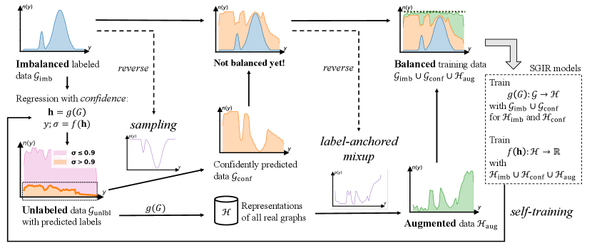
Figure 1 illustrates our ideas to overcome the above challenges. First, we want to progressively reduce the model bias by gradually improving training data from the labeled and unlabeled sets. The performance of pseudo-labeling models and the quality of the expanded training data can mutually enhance each other through iterations. Second, we relate the regression confidence to the prediction variance under perturbations. Higher confidence indicates a lower prediction variance under different perturbation environments. Therefore, we define and use regression confidence score to avoid pseudo-label noise and select quality examples in regression tasks. To fully exploit the quality pseudo-labels to compensate for the data imbalance in different label ranges, we use a reversed distribution of the imbalanced annotated data to reveal label ranges that need to be more or less selected for label balancing. Third, we attempt to achieve the perfect balance of training data by creating graph examples of any given label value in the remaining under-represented ranges.

In this paper, we propose SGIR, a novel Semi-supervised framework for Graph Imbalanced Regression. This framework has three novel designs to implement our ideas. First, SGIR is a self-training framework with multiple iterations for model learning and balanced training data generation. Our second design is to sample more quality pseudo-labels for the less represented label ranges. We define a new measurement of regression confidence from recent studies on graph rationalization methods which provide perturbations for predictions at training and inference. After applying the confidence to filter out pseudo-label noise, we adopt reverse sampling to find optimal sampling rates at each label value that maximize the possibility of data balance. Intuitively, if a label value is less frequent in the annotated data, the sampling rate at this value is bigger and more pseudo-labeled examples are selected for model training. Third, we design a novel label-anchored mixup algorithm to augment graph examples by mixing up a virtual data point and a real graph example in latent space. Each virtual point is anchored at a certain label value that is still rare in the expanded labeled data. The mixed-up graph representations continue complementing the label ranges where we seriously lack data examples.

To empirically demonstrate the advantage of SGIR, we conduct experiments on seven graph property regression tasks from three different domains. Results show that SGIR significantly reduces the prediction error on all the tasks and in both under-/well-represented label ranges. For example, on the smallest dataset Mol-FreeSolv that has only 276 annotated graphs, SGIR reduces the mean absolute error from 1.114 to 0.777 (relatively 30% improvement) in the most under-represented label range and reduces the error from 0.642 to 0.563 (12% improvement) in the entire label space compared to state-of-the-art graph regression methods. To summarize:

•

We address a new problem of graph imbalance regression with a novel semi-supervised framework SGIR.
•

SGIR is a novel self-training framework creating balanced and enriched training data from pseudo-labels and augmented examples with three collaborated components: regression confidence, reverse sampling, and label-anchored mixup.
•

SGIR is theoretically motivated and empirically validated on seven graph regression tasks. It outperforms other semi-supervised learning and imbalanced regression methods in both well-represented and under-represented label ranges.

2. Related Work

2.1. Imbalanced Learning

Data resampling is known as under-sampling majority classes or over-sampling minority classes. SMOTE (Chawla et al., 2002) created synthetic data for minority classes using linear interpolations on labeled data. Cost-sensitive techniques (Cui et al., 2019; Lin et al., 2017) assigned higher weights to the loss of minority classes. And posterior re-calibration (Cao et al., 2019; Tian et al., 2020; Menon et al., 2021) encouraged larger margins for the prediction logits of minority classes. Imbalanced regression tasks have unique challenges due to continuous label values (Yang et al., 2021). Some of the methods from imbalanced classifications were extended to imbalanced regression tasks. For example, SMOGN (Branco et al., 2017) adopted the idea and method of SMOTE for regression; Recently, Yang et al. (2021) used regression focal loss and cost-sensitive reweighting; and BMSE (Ren et al., 2022) used logit re-calibration to predict numerical labels. LDS (Yang et al., 2021) smoothed label distribution using kernel density estimation. RankSim (Gong et al., 2022) regularized the latent space by approximating the distance of data points in the label space. Although these methods would improve performance on under-represented labels, they come at the expense of decreased performance on well-represented labels, particularly when annotated data is limited. SGIR avoids this by using unlabeled graphs to create more labels in the under-represented label ranges.

2.2. Semi-supervised Learning

To exploit unlabeled data, semi-supervised image classifiers such as FixMatch (Sohn et al., 2020) and MixMatch (Berthelot et al., 2019) used pseudo-labeling and consistency regularization. Their performance relies on weak and strong data augmentation techniques, which are under-explored for regression tasks and graph property prediction tasks. At the same time, semi-supervised learners suffer from the model bias caused by the unlabeled imbalance. Therefore, after pseudo-labeling unlabeled data, DARP (Kim et al., 2020) and DASO (Oh et al., 2022) refined the biased pseudo-labels by aligning their distribution with an approximated true class distribution of unlabeled data. CADR (Hu et al., 2022) adjusted the threshold for pseudo-label assignments. CReST (Wei et al., 2021) selected more pseudo-labels for minority classes in self-training. To the best of our knowledge, there was no work that leveraged unlabeled data for regression tasks on imbalanced graph data, although SSDKL (Jean et al., 2018) performed semi-supervised regression for non-graph data without considering label imbalance. SGIR makes the first attempt to solve the imbalanced regression problem using semi-supervised learning.

2.3. Graph Property Prediction

Graph neural network models (GNN) (Kipf and Welling, 2017; Veličković et al., 2018; Hamilton et al., 2017; Xu et al., 2019) have demonstrated their power for regression tasks in the fields of biology, chemistry, and material science (Hu et al., 2022; Liu et al., 2022). Data augmentation (Zhao et al., 2022a; Liu et al., 2023a) is an effective way to exploit limited labeled data. The node- and link-level augmentations (Rong et al., 2019; Zhao et al., 2021b, 2022b) modified graph structure to improve the accuracy of node classification and link prediction. On the graph level, augmentation methods were mostly designed for classification (Han et al., 2022; Wang et al., 2021). Recently, GREA (Liu et al., 2022) delivered promising results for predicting polymer properties. But the model bias caused by imbalanced continuous labels was not addressed. InfoGraph (Sun et al., 2020) exploited unlabeled graphs, however, the data imbalance issue was not addressed either. Our work aims to achieve balanced training data for graph regression in real practice where we have a small set of imbalanced labeled graphs and a large set of unlabeled data.

3. Problem Definition

To predict the property $y\in\mathbb{R}$ of a graph $G\in\mathcal{G}$ , a graph regression model usually consists of an encoder $g:G\rightarrow\mathbf{h}\in\mathbb{R}^{d}$ and a decoder $f:\mathbf{h}\rightarrow\hat{y}\in\mathbb{R}$ . The encoder $g(\cdot)$ is often a graph neural network (GNN) that outputs the $d$ -dimensional representation vector $\mathbf{h}$ of graph $G$ , and the decoder $f(\cdot)$ is often a multi-layer perceptron (MLP) that makes the label prediction $\hat{y}$ given $\mathbf{h}$ .

Let $\mathcal{G}_{\text{imb}}=\{(G_{i},y_{i})\}_{i=1}^{n_{\text{imb}}}$ denote the labeled training data for graph regression models, where $n_{\text{imb}}$ is the number of training graphs in the imbalanced labeled dataset. It often concentrates on certain areas in the continuous label space. To reveal it, we first divide the label space into $C$ intervals and use them to fully cover the range of continuous label values. These intervals are $[b_{0},b_{1}),[b_{1},b_{2}),\dots,[b_{C-1},b_{C})$ . Then, we assign the labeled examples into $C$ intervals and count them in each interval to construct the frequency set $\{\mu_{i}\}_{i=1}^{C}$ . We could find that $\frac{\max\{\mu_{i}\}}{\min\{\mu_{i}\}}\gg 1$ (i.e., label imbalance) often exists, instead of $\mu_{1}=\mu_{2}=\dots=\mu_{C}$ (i.e., label balance) that is assumed by most existing models. The existing models may be biased to small areas in the label space that are dominated by the majority of labeled data and lack a good generalization to areas that are equally important but have much fewer examples.

Labeling continuous graph properties is difficult (Yuan et al., 2021), limiting the size of labeled data. Fortunately, a large number of unlabeled graphs are often available though ignored in most existing studies. In this work, we aim to use the unlabeled examples to alleviate the label imbalance issue in graph regression tasks. That is, let $\mathcal{G}_{\text{unlbl}}=\{G_{j}\}_{j=n_{\text{imb}}+1}^{n_{\text{imb}}+n_{\text{unlbl}}}$ denote the $n_{\text{unlbl}}$ available unlabeled graphs. We want to train $g(\cdot)$ and $f(\cdot)$ to deliver good performance through the whole continuous label space by utilizing both $\mathcal{G}_{\text{imb}}$ and $\mathcal{G}_{\text{unlbl}}$ .

4. Proposed Framework

To progressively reduce label imbalance bias, we propose a novel framework named SGIR that iteratively creates reliable labeled examples in the areas of label space where annotations were not frequent. As presented in Figure 1, SGIR uses a graph regression model to create the labels and uses the gradually balanced data to train the regression model. To let data balancing and model construction mutually enhance each other, SGIR is a self-training framework that trains the encoder $g(\cdot)$ and decoder $f(\cdot)$ using two strategies through multiple iterations. The first strategy is to use pseudo-labels based on confident predictions and reverse sampling, leveraging unlabeled data (see Section 4.2). Because the unlabeled graph set still may not contain real examples of rare label values, the second strategy is to augment the graph representation examples for the rare areas using a novel label-anchored mixup algorithm (see Section 4.3).

4.1. A Self-Training Framework for Iteratively Balancing Scalar Label Data

A classic self-training framework is expected to be a virtuous circle exploiting the unlabeled data in label-balanced classification/regression tasks (Xie et al., 2020; McLachlan, 1975). It first trains a classifier/regressor that iteratively assigns pseudo-labels to the set of unlabeled training examples $\mathcal{G}_{\text{unlbl}}$ with a margin greater than a certain threshold. The pseudo-labeled examples are then used to enrich the labeled training set. And the classifier continues training with the updated training set. For a virtuous circle of model training with imbalanced labeled set $\mathcal{G}_{\text{imb}}$ , the most confident predictions on $\mathcal{G}_{\text{unlbl}}$ should be selected to compensate for the under-represented labels, as well as to enrich the dataset $\mathcal{G}_{\text{imb}}$ . In each iteration, the model becomes less biased to the majority of labels. And the less biased model can make predictions of higher accuracy and confidence on the unlabeled data. Therefore, we hypothesize that model training and data balancing can mutually enhance each other.

SGIR is a self-training framework targeting to generalize the model performance everywhere in the continuous label space with particularly designed balanced training data from the labeled graph data $\mathcal{G}_{\text{imb}}$ , confidently selected graph data $\mathcal{G}_{\text{conf}}$ , and augmented representation data $\mathcal{H}_{\text{aug}}$ . For the next round of model training, the gradually balanced training data reduce the label imbalance bias carried by the graph encoder $g(\cdot)$ and decoder $f(\cdot)$ . Then the less biased graph encoder and decoder are applied to generate balanced training data of higher quality. Through these iterations, the model bias from the imbalanced or low-quality balanced data would be progressively reduced because of the gradually enhanced quality of balanced training data.

4.2. Balancing with Confidently Predicted Labels

At each iteration, SGIR enriches and balances training data with pseudo-labels of good quality. The unlabeled data examples in $\mathcal{G}_{\text{unlbl}}$ are firstly exploited by reliable and confident predictions. Then the reverse sampling from the imbalanced label distribution of original training data $\mathcal{G}_{\text{imb}}$ is used to select more pseudo-labels for under-represented label ranges.

4.2.1. Graph regression with confidence

A standard regression model outputs a scalar without a certain definition of confidence of its prediction. The confidence is often measured by how much the predicted probability is close to 1 in classifications. The lack of confidence measurements in graph regression tasks may introduce noise to the self-training framework that aims at label balancing. It would be more severe when the domain gap exists between labeled and unlabeled data (Berthelot et al., 2022). Recent studies (Liu et al., 2022; Wu et al., 2022) have proposed two concepts that help us define a good measurement: rationale subgraph and environment subgraph. A rationale subgraph is supposed to best support and explain the prediction at property inference. Its counterpart environment subgraph is the complementary subgraph in the example, which perturbs the prediction from the rationale subgraph if used. Our idea is to measure the confidence of graph property prediction based on the reliability of the identified rationale subgraphs. Specifically, we use the variance of predicted label values from graphs that consist of a specific rationale subgraph and one of many possible environment subgraphs.

We use an existing supervised graph regression model that can identify rationale and environment subgraphs in any graph example to predict its property. We denote $G_{i}$ as the $i$ -th graph in a batch of size $B$ . The model separates $G_{i}$ into $G^{(r)}_{i}$ and $G^{(e)}_{i}$ . For the $j$ -th graph $G_{j}$ in the same batch, we have a combined example $G_{(i,j)}=G^{(r)}_{i}\cup G^{(e)}_{j}$ that has the rationale of $G_{i}$ and environment subgraph of $G_{j}$ . So it is expected to have the same label of $G_{i}$ . By enumerating $j\in\{1,2,\dots,B\}$ , the encoder $g(\cdot)$ and decoder $f(\cdot)$ are trained to predict the label value of any $G_{(i,j)}$ . We define the confidence of predicting the label of $G_{i}$ as:

(1)

\sigma_{i}=\frac{1}{\operatorname{Var}\left(~{}{\{f(g(G_{(i,j)}))\}}_{j=1,2,\dots,B}~{}\right)}.

It is the reciprocal of prediction variance. In implementation, we choose GREA (Liu et al., 2022) as the model. Considering efficiency, GREA creates $G_{(i,j)}$ in the latent space without decoding its graph structure. That is, it directly gets the representation of $G_{(i,j)}$ as the sum of the representation vectors $\mathbf{h}^{(r)}_{i}$ of $G^{(r)}_{i}$ and $\mathbf{h}^{(e)}_{j}$ of $G^{(e)}_{j}$ . So we have

(2)

\sigma_{i}=\frac{1}{\operatorname{Var}\left(~{}{\{f(\mathbf{h}^{(r)}_{i}+\mathbf{h}^{(e)}_{j})\}}_{j=1,2,\dots,B}~{}\right)}.

Now we have predicted labels and confidence values for graph examples in the large unlabeled dataset $\mathcal{G}_{\text{unlbl}}$ . Examples with low confidences will bring noise to the training data if we use them all. So we only consider a data example $G_{i}$ to be of good quality if its confidence $\sigma_{i}$ is not smaller than a threshold $\tau$ . We name this confidence measurement based on graph rationalization as GRation. GRation is tailored for graph regression tasks by considering the environment subgraphs as perturbations. We will compare its effect on quality graph selection against other graph-irrelevant methods such as Dropout (Gal and Ghahramani, 2016), Certi (Tagasovska and Lopez-Paz, 2019), DER (Deep Evidential Regression) (Amini et al., 2020), and Simple (no confidence) in experiments.

After leveraging the unlabeled data, the label distribution of quality examples may still be biased to the majority of labels. So we further apply reverse sampling on these examples from $\mathcal{G}_{\text{unlbl}}$ to balance the distribution of training data.

4.2.2. Reverse sampling

The reverse sampling in SGIR helps reduce the model bias to label imbalance. Specifically, we want to selectively add unlabeled examples predicted in the under-represented label ranges. Suppose we have the frequency set $\{\mu_{i}\}_{i=1}^{C}$ of $C$ intervals. We denote $p_{i}$ as the sampling rate at the $i$ -th interval and follow Wei et al. (2021) to calculate it. Basically, to perform reverse sampling, we want $p_{i}<p_{j}$ if $\mu_{i}>\mu_{j}$ . We define a new frequency set $\{\mu^{\prime}_{i}\}_{i=1}^{C}$ in which $\mu^{\prime}_{i}$ equals the $i$ -th smallest in $\{\mu\}$ if $\mu_{i}$ is the $i$ -th biggest in $\{\mu\}$ . Then the sampling rate is

(3)

p_{i}=\frac{\mu^{\prime}_{i}}{\max\{\mu_{1},\mu_{2},\dots,\mu_{C}\}}.

To this end, we have the confidently labeled and reversed sampled data $\mathcal{G}_{\text{conf}}$ . In each self-training iteration, we combine it with the original training set $\mathcal{G}_{\text{imb}}$ .

4.3. Balancing with Augmentation via Label-Anchored Mixup

Although $\mathcal{G}_{\text{imb}}\cup\mathcal{G}_{\text{conf}}$ is more balanced than $\mathcal{G}_{\text{imb}}$ , we observe that $\mathcal{G}_{\text{imb}}\cup\mathcal{G}_{\text{conf}}$ is usually far from a perfect balance, even if $\mathcal{G}_{\text{unlbl}}$ could be hundreds of times bigger than $\mathcal{G}_{\text{imb}}$ . To create graph examples targeting the remaining under-represented label ranges, we design a novel label-anchored mixup algorithm for graph imbalanced regression. Compared to existing mixup algorithms (Wang et al., 2021; Verma et al., 2019) for classifications without awareness of imbalance, our new algorithm can augment training data with additional examples for target ranges of continuous label value.

A mixup operation in the label-anchored mixup is to mix up two things in a latent space: (1) a virtual data point representing an interval of targeted label and (2) a real graph example. Specifically, we first calculate the representation of a target label interval by averaging the representation vectors of graphs in the interval from the labeled dataset $\mathcal{G}_{\text{imb}}$ . Let $\mathbf{M}\in{\{0,1\}}^{C\times n_{\text{imb}}}$ be an indicator matrix, where $M_{i,j}=1$ means that the label of $G_{j}\in\mathcal{G}_{\text{imb}}$ belongs to the $i$ -th interval. We denote $\mathbf{H}\in\mathbb{R}^{n_{\text{imb}}\times d}$ as the matrix of graph representations from the GNN encoder $g(\cdot)$ for $\mathcal{G}_{\text{imb}}$ . The representation matrix $\mathbf{Z}\in\mathbb{R}^{C\times d}$ of all intervals is calculated

(4)

\mathbf{Z}=\operatorname{norm}(\mathbf{M})\cdot\mathbf{H},

where $\operatorname{norm}(\cdot)$ is the row-wise normalization. Let $a_{i}$ denote the center label value of the $i$ -th interval. Then we have the representation-label pairs of all the label intervals $\{(\mathbf{z}_{i},a_{i})\}_{i=1}^{C}$ , where $\mathbf{z}_{i}$ is the $i$ -th row of $\mathbf{Z}$ .

Now we can use each interval center $a_{i}$ as a label anchor to augment graph data examples in a latent space. We select $n_{i}\propto p_{i}$ real graphs from $\mathcal{G}_{\text{imb}}\cup\mathcal{G}_{\text{conf}}$ whose labels are closest to $a_{i}$ , where $p_{i}$ is calculated by Eq. 3. The more real graphs are selected, the more graph representations are augmented. $n_{i}$ is likely to be big when the label anchor $a_{i}$ remains under-represented after $\mathcal{G}_{\text{conf}}$ is added to training set. Note that the labels were annotated if the graphs were in $\mathcal{G}_{\text{imb}}$ and predicted if they were in $\mathcal{G}_{\text{unlbl}}$ . For $j\in\{1,2,\dots,n_{i}\}$ , we mix up the interval ( $\mathbf{z}_{i}$ , $a_{i}$ ) and a real graph ( $\mathbf{h}_{j}$ , $y_{j}$ ), where $\mathbf{h}_{j}$ and $y_{i}$ are the representation vector and the annotated or predicted label of the $j$ -th graph, respectively. Then the mixup operation is defined as

(5)

\begin{cases}\tilde{\mathbf{h}}_{(i,j)}&=\lambda\cdot\mathbf{z}_{i}+\big{(}1-\lambda\big{)}\cdot\mathbf{h}_{j},\\ \tilde{y}_{(i,j)}&=\lambda\cdot a_{i}+\big{(}1-\lambda\big{)}\cdot y_{j},\\ \end{cases}

where $\tilde{\mathbf{h}}_{(i,j)}$ and $\tilde{y}_{(i,j)}$ are the representation vector and label of the augmented graph, respectively. $\lambda=\max(\lambda^{\prime},1-\lambda^{\prime})$ , $\lambda^{\prime}\sim\text{Beta}(1,\beta)$ , and $\beta$ is a hyperparameter. $\lambda$ is often closer to 1 because we want $\tilde{y}_{(i,j)}$ to be closer to the label anchor $a_{i}$ . Let $\mathcal{H}_{\text{aug}}$ denote the set of representation vectors of all the augmented graphs. Combined with $\mathcal{G}_{\text{imb}}$ and $\mathcal{G}_{\text{conf}}$ , we end up with a label-balanced training set for the next round of self-training.

4.4. Optimization

In each iteration of self-training, we jointly optimize the parameters of graph encoder $g(\cdot)$ and label predictor $f(\cdot)$ with a gradually balanced training set $\mathcal{G}_{\text{imb}}\cup\mathcal{G}_{\text{conf}}\cup\mathcal{H}_{\text{aug}}$ .

We use the mean absolute error (MAE) as the regression loss. Specifically, for each $(G,y)\in\mathcal{G}_{\text{imb}}\cup\mathcal{G}_{\text{conf}}$ , the loss is $\ell_{\text{imb+conf}}=\operatorname{MAE}(f(g(G)),y)$ . Given $(\mathbf{h},y)\in\mathcal{H}_{\text{aug}}$ , the loss is $\ell_{\text{aug}}=\operatorname{MAE}(f(\mathbf{h}),y)$ . So the total loss for SGIR is

\mathcal{L}=\sum_{(G,y)\in\mathcal{G}_{\text{imb}}\cup\mathcal{G}_{\text{conf}}}\ell_{\text{imb+conf}}(G,y)+\sum_{(\mathbf{h},y)\in\mathcal{H}_{\text{aug}}}\ell_{\text{aug}}(\mathbf{h},y).

Our framework is flexible with any graph encoder-decoder models. To be consistent and given the promising results in graph regression tasks, we use the design of graph encoder and decoder in GREA (Liu et al., 2022) which is also used for measuring prediction confidence in Eq. 2.

4.5. Theoretical Motivations

There is a lack of theoretical principle for imbalanced regression. Our theoretical motivation extends the generalization error bound from classification (Cao et al., 2019) to regression. The original bound enforces bigger margins for minority classes, which potentially hurt the model performance for well-represented classes (Tian et al., 2020; Zhang et al., 2023). Our result provides a more safe way to reduce the error bound by utilizing unlabeled graphs with self-training in graph regression tasks.

As we divide the label distribution into $C$ intervals, every graph example can be assigned into an interval (as the ground-truth interval) according to the distance between the interval center and the ground-truth label value. Besides, we use $S_{[b_{i},b_{i+1})}(G)$ to denote the reciprocal of the distance between the predicted label of the graph $G$ and the $i$ -th interval $[b_{i},b_{i+1})$ , where $i\in\{1,2,\dots,C\}$ . In this way, we could define $f(\cdot)$ as a regression function that outputs a continuous predicted label. Then $S_{[b_{i},b_{i+1})}(G)$ consists of $f(\cdot)$ and outputs the logits to classify the graph to the $i$ -the interval.

We consider all training examples to follow the same distribution. We assume that conditional on label intervals, the distributions of graph sampling are the same at training and testing stages. So, the standard 0-1 test error on the balanced test distribution is

(6)

\mathcal{E}_{\textup{bal}}\left[f\right]=\underset{\left(G,[b_{i},b_{i+1})\right)\sim\mathcal{P}_{\textup{bal}}}{\operatorname{Pr}}\left[S_{[b_{i},b_{i+1})}(G)<\max_{j\neq i}S_{[b_{j},b_{j+1})}(G)\right],

where $\mathcal{P}_{\textup{bal}}$ denotes the balanced test distribution. It first samples a label interval uniformly and then samples graphs conditionally on the interval. The error for the $i$ -th interval $[b_{i},b_{i+1})$ is defined as

(7)

\mathcal{E}_{[b_{i},b_{i+1})}\left[f\right]=\underset{G\sim\mathcal{P}_{[b_{i},b_{i+1})}}{\operatorname{Pr}}\left[S_{[b_{i},b_{i+1})}(G)<\max_{j\neq i}S_{[b_{j},b_{j+1})}(G)\right],

where $\mathcal{P}_{[b_{i},b_{i+1})}$ denotes the distribution for the interval ${[b_{i},b_{i+1})}$ . We define $\gamma\left(G,[b_{i},b_{i+1})\right)=S_{[b_{i},b_{i+1})}(G)-\max_{j\neq i}S_{[b_{j},b_{j+1})}(G)$ as the margin of an example $G$ assigned to the interval $[b_{i},b_{i+1})$ . To define the training margin $\gamma_{{}_{[b_{i},b_{i+1})}}$ for the interval $[b_{i},b_{i+1})$ , we calculate the minimal margin across all examples assigned to that interval:

(8)

\gamma_{{}_{[b_{i},b_{i+1})}}=\min_{G_{j}\in[b_{i},b_{i+1})}\gamma\left(G_{j},[b_{i},b_{i+1})\right).

We assume that the $\operatorname{MAE}$ regression loss is small enough to correctly assign all training examples to the corresponding intervals. Given the hypothesis class $\mathcal{F}$ , $\textup{C}(\mathcal{F})$ is assumed to be a proper complexity measure of $\mathcal{F}$ . We assume there are $n_{[b_{i},b_{i+1})}$ examples i.i.d sampled from the conditional distribution $\mathcal{P}_{[b_{i},b_{i+1})}$ for the interval $[b_{i},b_{i+1})$ . So, we apply the standard margin-based generalization bound to obtain the following theorem (Kakade et al., 2008; Cao et al., 2019; Zhao et al., 2021a):

Theorem 4.1.

With probability ( $1-\delta$ ) over the randomness of the training data, the error $\mathcal{E}_{[b_{i},b_{i+1})}$ for interval $[b_{i},b_{i+1})$ is bounded by

(9)

\begin{split}\mathcal{E}_{[b_{i},b_{i+1})}[f]&\lessapprox\frac{1}{\gamma_{{}_{[b_{i},b_{i+1})}}}\sqrt{\frac{\textup{C}(\mathcal{F})}{n_{[b_{i},b_{i+1})}}}\\ &+\sqrt{\frac{\log\log_{2}(1/\gamma_{{}_{[b_{i},b_{i+1})}})+\log(1/\delta)}{n_{[b_{i},b_{i+1})}}},\end{split}

where $\lessapprox$ hides constant terms. Taking union bound over all intervals, we have $\mathcal{E}_{\textup{bal}}[f]\lessapprox\frac{1}{C}\sum_{i=1}^{C}\mathcal{E}_{[b_{i},b_{i+1})}[f]$ .

Proofs are in appendix B. The bound decreases as the increase of the examples in corresponding label ranges. The SGIR is motivated to reduce and balance the bound for different intervals by manipulating $n_{[b_{i},b_{i+1})}$ with pseudo-labels and augmented examples. Particularly, we discuss in Section B.3 that the augmented examples do not break our assumption for the theorem and future directions of imbalanced regression theories without intervals.

5. Experiments

Table 1. Statistics of six tasks for graph property regression.

Dataset	# Graphs (Train/Valid/Test)	# Nodes (Avg./Max)	# Edges (Avg./Max)
Mol-Lipo	2,048 / 1,076 / 1,076	27.0 / 115	59.0 / 236
Mol-ESOL	446 / 341 / 341	13.3 / 55	27.4 / 125
Mol-FreeSolv	276 / 183 / 183	8.7 / 24	16.8 / 50
Plym-Melting	2,419 / 616 / 616	26.9 / 102	55.4 / 212
Plym-Density	844 / 425 / 425	27.3 / 93	57.6 / 210
Plym-Oxygen	339 / 128 / 128	37.3 / 103	82.1 / 234
Superpixel-Age	3619 / 628 / 628	67.9 / 75.0	265.6 / 300

Table 2. Results of Mean(Std) on six molecule/polymer datasets. The best mean is bolded. The best baseline is underlined.

		MAE $\downarrow$				GM $\downarrow$
		All	Many-shot	Med.-shot	Few-shot	All	Many-shot	Med.-shot	Few-shot
Mol-Lipo	GNN	0.485(0.010)	0.421(0.030)	0.462(0.013)	0.566(0.032)	0.297(0.012)	0.252(0.022)	0.294(0.016)	0.348(0.030)
	RankSim	0.475(0.018)	0.388(0.017)	0.438(0.007)	0.587(0.043)	0.297(0.015)	0.249(0.017)	0.274(0.006)	0.380(0.044)
	BMSE	0.494(0.007)	0.409(0.019)	0.450(0.007)	0.614(0.033)	0.304(0.008)	0.260(0.014)	0.279(0.015)	0.382(0.038)
	LDS	0.468(0.009)	0.394(0.012)	0.449(0.012)	0.551(0.026)	0.294(0.010)	0.251(0.009)	0.281(0.010)	0.356(0.033)
	InfoGraph	0.499(0.008)	0.421(0.024)	0.471(0.013)	0.596(0.026)	0.314(0.011)	0.269(0.018)	0.300(0.006)	0.376(0.029)
	GREA	0.487(0.002)	0.391(0.015)	0.434(0.008)	0.626(0.018)	0.294(0.010)	0.251(0.009)	0.281(0.010)	0.356(0.033)
	SGIR	0.432(0.012)	0.357(0.019)	0.413(0.017)	0.515(0.020)	0.264(0.013)	0.224(0.016)	0.256(0.017)	0.314(0.015)
Mol-ESOL	GNN	0.508(0.015)	0.398(0.018)	0.448(0.012)	0.696(0.025)	0.299(0.017)	0.231(0.017)	0.279(0.014)	0.425(0.035)
	RankSim	0.501(0.014)	0.389(0.021)	0.443(0.019)	0.689(0.025)	0.293(0.021)	0.227(0.028)	0.258(0.020)	0.449(0.030)
	BMSE	0.533(0.023)	0.400(0.027)	0.449(0.015)	0.777(0.069)	0.308(0.018)	0.245(0.036)	0.266(0.009)	0.473(0.035)
	LDS	0.517(0.016)	0.423(0.012)	0.474(0.029)	0.668(0.010)	0.304(0.010)	0.261(0.007)	0.283(0.025)	0.393(0.009)
	InfoGraph	0.561(0.025)	0.475(0.034)	0.466(0.036)	0.776(0.036)	0.336(0.014)	0.306(0.022)	0.276(0.013)	0.484(0.029)
	GREA	0.497(0.031)	0.396(0.040)	0.456(0.033)	0.652(0.045)	0.289(0.032)	0.226(0.038)	0.270(0.025)	0.404(0.051)
	SGIR	0.457(0.015)	0.370(0.022)	0.411(0.011)	0.604(0.024)	0.263(0.016)	0.226(0.021)	0.240(0.015)	0.347(0.030)
Mol-FreeSolv	GNN	0.726(0.039)	0.617(0.061)	0.695(0.055)	1.154(0.082)	0.363(0.025)	0.317(0.027)	0.360(0.029)	0.556(0.073)
	RankSim	0.779(0.109)	0.764(0.225)	0.674(0.072)	1.220(0.146)	0.367(0.026)	0.396(0.052)	0.315(0.030)	0.537(0.082)
	BMSE	0.856(0.071)	0.809(0.117)	0.820(0.064)	1.122(0.076)	0.456(0.042)	0.426(0.029)	0.457(0.054)	0.552(0.062)
	LDS	0.809(0.071)	0.796(0.071)	0.737(0.088)	1.114(0.141)	0.443(0.045)	0.489(0.036)	0.387(0.052)	0.580(0.146)
	InfoGraph	0.933(0.042)	0.830(0.081)	0.913(0.030)	1.308(0.171)	0.542(0.048)	0.505(0.107)	0.528(0.038)	0.789(0.183)
	GREA	0.642(0.026)	0.541(0.064)	0.570(0.008)	1.202(0.023)	0.321(0.038)	0.294(0.064)	0.301(0.024)	0.537(0.049)
	SGIR	0.563(0.026)	0.535(0.038)	0.528(0.046)	0.777(0.061)	0.264(0.029)	0.286(0.013)	0.244(0.046)	0.304(0.078)
Plym-Melting	GNN	41.8(1.2)	35.5(1.2)	33.0(0.7)	54.7(2.2)	23.2(1.0)	21.3(1.1)	16.2(1.0)	33.4(2.5)
	RankSim	41.1(0.9)	34.1(0.5)	33.6(1.1)	53.5(1.2)	22.6(1.1)	20.5(0.5)	16.8(1.0)	31.4(2.8)
	BMSE	42.1(0.7)	35.8(1.4)	34.1(1.3)	54.4(1.5)	23.7(1.2)	21.5(1.0)	18.1(0.5)	32.4(3.0)
	LDS	41.6(0.3)	35.3(0.9)	34.5(1.1)	53.2(0.8)	23.2(0.2)	20.5(1.2)	18.3(0.5)	31.4(1.1)
	InfoGraph	43.6(2.8)	35.3(2.3)	35.0(2.3)	58.3(4.1)	24.6(1.9)	21.3(1.5)	18.4(1.5)	35.4(4.1)
	GREA	41.2(0.8)	33.3(0.5)	32.7(0.7)	55.3(3.0)	23.4(0.6)	20.0(0.6)	17.3(0.7)	34.3(2.9)
	SGIR	38.9(0.7)	31.7(0.3)	31.5(1.1)	51.4(1.6)	21.1(1.2)	18.5(0.5)	15.9(1.4)	30.2(1.9)
Plym-Density	GNN	61.2(5.4)	63.4(18.9)	46.6(1.6)	72.0(2.8)	29.3(0.6)	29.6(3.3)	23.5(0.9)	35.5(2.0)
	RankSim	57.5(1.8)	55.1(2.2)	46.3(1.8)	69.4(3.3)	29.3(1.6)	29.9(2.8)	23.1(2.1)	35.4(2.5)
	BMSE	61.8(2.0)	59.1(8.6)	48.2(2.0)	75.9(3.5)	31.9(1.3)	31.8(4.2)	26.3(2.2)	38.2(3.2)
(scaled: $\times 1,000$ )	LDS	60.1(2.4)	60.4(6.2)	47.0(1.3)	71.3(2.5)	31.5(2.0)	33.2(3.5)	24.4(3.0)	38.0(2.4)
	InfoGraph	54.9(1.7)	46.8(1.0)	43.0(1.9)	72.3(3.2)	29.3(1.8)	27.3(1.4)	22.6(1.2)	39.2(4.3)
	GREA	60.3(1.9)	49.0(4.4)	48.1(2.5)	80.7(4.2)	32.3(1.6)	26.7(2.7)	27.2(2.3)	44.7(6.1)
	SGIR	53.0(0.5)	45.4(1.7)	42.5(2.8)	68.6(2.6)	26.6(0.4)	24.0(2.2)	23.0(1.3)	33.4(3.0)
Plym-Oxygen	GNN	183.5(33.4)	6.3(3.2)	14.6(6.6)	464.0(85.3)	7.0(1.8)	2.4(0.7)	3.9(1.1)	29.9(7.2)
	RankSim	165.7(27.4)	3.9(1.4)	13.0(2.0)	420.7(69.7)	5.9(1.4)	1.8(0.3)	3.6(1.7)	26.6(6.7)
	BMSE	190.4(33.4)	26.4(21.6)	27.0(16.4)	454.3(88.9)	25.7(14.8)	14.9(11.7)	15.9(9.6)	63.2(23.5)
	LDS	180.0(23.0)	6.6(4.0)	11.8(2.0)	456.3(60.2)	7.6(1.6)	2.4(0.6)	4.7(1.4)	33.6(9.2)
	InfoGraph	199.5(31.5)	7.5(7.2)	13.0(1.8)	505.5(78.2)	7.8(1.9)	2.3(0.5)	5.1(2.2)	34.8(8.5)
	GREA	182.5(30.0)	9.0(8.6)	14.4(4.9)	458.8(79.2)	7.1(1.3)	2.1(0.5)	4.4(1.3)	31.7(5.0)
	SGIR	150.9(17.8)	3.8(1.1)	12.2(0.6)	382.8(46.9)	5.8(0.4)	2.1(0.7)	3.3(0.8)	24.4(6.8)

We conduct experiments to demonstrate the effectiveness of SGIR and answer the research question: how it performs on graph regression tasks and at different label ranges (RQ1). We also make a few ablation studies to investigate the effect of model design: where the effectiveness comes from (RQ2).

5.1. Experimental Settings

5.1.1. Datasets

MAE $\downarrow$		GM $\downarrow$
GNN	14.583(0.413)	10.524(0.994)	11.698(0.404)	22.127(0.780)	9.996(0.386)	7.265(0.858)	7.910(0.492)	18.404(0.673)
RankSim	14.464(0.401)	10.468(0.759)	11.610(0.774)	21.910(0.700)	9.606(0.303)	6.936(0.598)	7.721(0.660)	17.534(1.768)
BMSE	15.179(0.594)	10.639(2.303)	12.201(0.900)	23.321(2.525)	10.419(0.393)	7.249(1.526)	8.659(0.827)	19.719(4.318)
LDS	14.674(0.191)	10.972(0.495)	11.985(0.627)	21.623(0.926)	9.867(0.291)	7.317(0.672)	7.997(0.633)	17.298(0.957)
InfoGraph	14.515(0.605)	10.610(1.063)	11.150(0.158)	22.476(1.147)	9.879(0.524)	7.391(0.995)	7.377(0.333)	18.969(1.873)
GREA	14.682(0.300)	10.283(0.503)	11.999(0.585)	22.329(0.570)	10.037(0.438)	7.051(0.455)	8.273(0.565)	18.142(1.276)
SGIR	13.787(0.123)	10.171(0.4156)	11.066(0.389)	20.687(0.839)	9.261(0.221)	6.928(0.355)	7.247(0.593)	16.769(1.418)

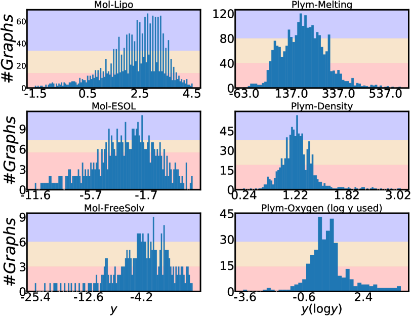
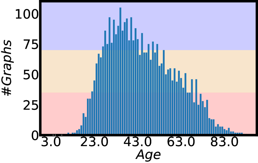
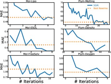
Molecule and polymer datasets in Table 1 (the datasets with a prefix Mol- or Plym-) and Figure 2 present detailed data statistics for six graph regression tasks from chemistry and materials science. Three molecule datasets are from (Wu et al., 2018) and three polymer datasets are from (Liu et al., 2022). Besides labeled graphs, we combine a database of 133,015 molecules in QM9 (Ramakrishnan et al., 2014) and an integration of four sets of 13,114 polymers in total (Liu et al., 2022) to create a set of 146,129 unlabeled graphs to set up semi-supervised graph regression. We note that the unlabeled graphs may be slightly less than 146,129 for a polymer task on Plym-Melting, Plym-Density or Plym-Oxygen. Because we remove the overlapping graph examples for the current polymer task with the polymer unlabeled data. We follow (Yang et al., 2021) to split the datasets to characterize imbalanced training distributions and balanced test distributions. The details of the age regression dataset are presented in Table 1 (Superpixel-Age) and Figure 3. The graph dataset Superpixel-Age is constructed from image superpixels using the algorithms from (Knyazev et al., 2019) on the image dataset AgeDB-DIR from (Moschoglou et al., 2017; Yang et al., 2021). Each face image in AgeDB-DIR has an age label from 0 to 101. We fisrt compute the SLIC superpixels for each image without losing the label-specific information (Achanta et al., 2012; Knyazev et al., 2019). Then we use the superpixels as nodes and calculate the spatial distance between superpixels to build edges for each image (Knyazev et al., 2019). Binary edges are constructed between superpixel nodes by applying a threshold on the top-5% of the smallest spatial distances. After building a graph for each image, the graph dataset Superpixel-Age consists of 3,619 graphs for training, 628 graphs for validation, 628 graphs for testing, and 11,613 unlabeled graphs for semi-supervised learning.

5.1.2. Evaluation metrics

We report model performance on three different sub-ranges following the work in (Yang et al., 2021; Ren et al., 2022; Gong et al., 2022), besides the entire range of label space. The three sub-ranges are the many-shot region, medium-shot region, and few-shot region. The sub-ranges are defined by the number of training graphs in each label value interval. Details for each dataset are presented in Figure 2 and Figure 3. To evaluate the regression performance, we use mean absolute error (MAE) and geometric mean (GM) (Yang et al., 2021). Lower values ( $\downarrow$ ) of MAE or GM indicate better performance.

Table 4. A comprehensive ablation study on molecule regression datasets with the metric MAE ( $\downarrow$ ). $\sigma$ is the confidence score in Section 4.2.1. $p$ is the reverse sampling in Section 4.2.2. ( $\tilde{\mathbf{h}}$ , $\tilde{y}$ ) is the label-anchored mixup in Section 4.3. aa $\sigma$ a a $p$ a ( $\tilde{\mathbf{h}}$ , $\tilde{y}$ ) All Many-shot Med.-shot Few-shot Mol-Lipo w/o $\mathcal{G}_{\text{unlbl}}$ 0.477(0.014) 0.378(0.030) 0.440(0.011) 0.600(0.006) ✓ ✗ ✗ 0.448(0.006) 0.371(0.004) 0.421(0.012) 0.543(0.016) ✗ ✓ ✗ 0.446(0.008) 0.356(0.003) 0.407(0.011) 0.564(0.016) ✓ ✓ ✗ 0.442(0.012) 0.372(0.007) 0.415(0.004) 0.533(0.026) ✗ ✗ ✓ 0.456(0.007) 0.372(0.014) 0.436(0.010) 0.549(0.005) ✓ ✓ ✓ 0.432(0.012) 0.357(0.019) 0.413(0.017) 0.515(0.020) Mol-ESOL w/o $\mathcal{G}_{\text{unlbl}}$ 0.477(0.027) 0.375(0.014) 0.432(0.042) 0.637(0.042) ✓ ✗ ✗ 0.475(0.014) 0.369(0.014) 0.446(0.017) 0.618(0.039) ✗ ✓ ✗ 0.480(0.017) 0.380(0.035) 0.440(0.017) 0.630(0.020) ✓ ✓ ✗ 0.468(0.007) 0.379(0.012) 0.425(0.013) 0.612(0.028) ✗ ✗ ✓ 0.474(0.010) 0.353(0.018) 0.450(0.009) 0.623(0.027) ✓ ✓ ✓ 0.457(0.015) 0.370(0.022) 0.411(0.011) 0.604(0.024) Mol-FreeSolv w/o $\mathcal{G}_{\text{unlbl}}$ 0.619(0.019) 0.525(0.022) 0.590(0.035) 1.000(0.072) ✓ ✗ ✗ 0.604(0.020) 0.557(0.037) 0.560(0.029) 0.903(0.055) ✗ ✓ ✗ 0.660(0.028) 0.574(0.015) 0.650(0.036) 0.941(0.066) ✓ ✓ ✗ 0.568(0.029) 0.538(0.020) 0.520(0.045) 0.831(0.132) ✗ ✗ ✓ 0.593(0.045) 0.536(0.033) 0.542(0.067) 0.947(0.062) ✓ ✓ ✓ 0.563(0.026) 0.535(0.038) 0.528(0.046) 0.777(0.061) Table 5. Investigation on choices of regression confidence with the metric MAE ( $\downarrow$ ). We disable all other SGIR components except the regression confidence score. Our confidence score (GRation) in Eq. 1 removes noise more effectively than others in graph regression tasks. Choice of $\sigma$ All Many-shot Med.-shot Few-shot Mol-Lipo Simple 0.481(0.010) 0.389(0.007) 0.440(0.013) 0.603(0.023) Dropout 0.450(0.026) 0.365(0.031) 0.420(0.022) 0.555(0.037) Certi 0.452(0.011) 0.384(0.018) 0.433(0.013) 0.532(0.010) DER 1.026(0.033) 0.604(0.035) 0.760(0.016) 1.672(0.111) GRation 0.448(0.006) 0.371(0.004) 0.421(0.012) 0.543(0.016) Mol-ESOL Simple 0.499(0.016) 0.397(0.023) 0.457(0.018) 0.656(0.033) Dropout 0.483(0.011) 0.381(0.027) 0.443(0.018) 0.636(0.027) Certi 0.487(0.030) 0.389(0.039) 0.439(0.024) 0.647(0.043) DER 0.918(0.135) 0.776(0.086) 0.826(0.098) 1.182(0.245) GRation 0.475(0.014) 0.369(0.014) 0.446(0.017) 0.618(0.039) Mol-FreeSolv Simple 0.697(0.056) 0.616(0.025) 0.663(0.033) 1.054(0.260) Dropout 0.639(0.013) 0.578(0.060) 0.589(0.017) 1.005(0.140) Certi 0.654(0.049) 0.589(0.046) 0.611(0.053) 0.999(0.130) DER 1.483(0.174) 1.180(0.162) 1.450(0.188) 2.480(0.373) GRation 0.604(0.020) 0.557(0.037) 0.560(0.029) 0.903(0.055)

5.1.3. Baselines and Implementations

Besides the GNN model, we broadly consider baselines from the fields of imbalanced regression and semi-supervised graph learning. Specifically, imbalanced regression baselines include LDS (Yang et al., 2021), BMSE (Ren et al., 2022), and RankSim (Gong et al., 2022). The semi-supervised graph learning baseline is InfoGraph (Sun et al., 2020) and the graph learning baseline is GREA (Liu et al., 2022). To implement SGIR and the baselines, the GNN encoder is GIN (Xu et al., 2019) and the decoder is a three-layer MLP to output property values. The threshold $\tau$ for selecting confident predictions is determined by the value at a certain percentile of the confidence score distribution. For all the methods, we reports the results on the test sets using the mean (standard deviation) over 10 runs with parameters that are randomly initialized. More Implementation details are in Appendix.

Table 6. Nine options on the implementation of the label-anchored mixup in Eq. 5. Except for the imbalanced labeled graphs

\mathcal{G}_{\text{imb}}

, the additional source of the interval representation

\textbf{z}_{i}

and the real graph representation

\textbf{h}_{j}

could be

\mathcal{G}_{\text{conf}}

\mathcal{G}_{\text{unlbl}}

. We extensively explore the options for

\mathcal{H}_{\text{aug}}

and find that source

\textbf{z}_{i}

from

\mathcal{G}_{\text{imb}}

and source

\textbf{h}_{j}

from

\mathcal{G}_{\text{unlbl}}

are usually the best.

$\textbf{z}_{i}$	$\textbf{h}_{j}$	Mol-Lipo				Plym-Oxygen
Additional Source		All	Many-shot	Med.-shot	Few-shot	All	Many-shot	Med.-shot	Few-shot
None	None	0.439(0.004)	0.361(0.010)	0.419(0.013)	0.529(0.022)	165.5(12.2)	4.7(1.7)	16.5(7.2)	417.4(31.1)
None	$\mathcal{G}_{\text{conf}}$	0.447(0.015)	0.359(0.004)	0.423(0.016)	0.549(0.033)	158.1(17.0)	4.1(0.7)	11.3(0.7)	401.9(45.1)
None	$\mathcal{G}_{\text{unlbl}}$	0.432(0.012)	0.357(0.019)	0.413(0.017)	0.515(0.020)	150.9(17.8)	3.8(1.1)	12.2(0.6)	382.8(46.9)
$\mathcal{G}_{\text{conf}}$	None	0.448(0.012)	0.367(0.008)	0.423(0.008)	0.544(0.028)	166.0(18.2)	11.9(11.3)	12.6(0.9)	414.0(52.6)
$\mathcal{G}_{\text{conf}}$	$\mathcal{G}_{\text{conf}}$	0.445(0.007)	0.364(0.008)	0.418(0.010)	0.542(0.012)	158.8(8.4)	7.7(8.9)	15.4(7.8)	397.5(15.4)
$\mathcal{G}_{\text{conf}}$	$\mathcal{G}_{\text{unlbl}}$	0.449(0.021)	0.360(0.023)	0.416(0.016)	0.560(0.039)	169.5(56.1)	4.5(1.2)	12.7(1.8)	430.4(145.0)
$\mathcal{G}_{\text{unlbl}}$	None	0.446(0.007)	0.367(0.009)	0.415(0.011)	0.546(0.011)	173.1(30.3)	3.7(0.4)	13.5(1.4)	440.0(79.3)
$\mathcal{G}_{\text{unlbl}}$	$\mathcal{G}_{\text{conf}}$	0.446(0.011)	0.368(0.011)	0.421(0.012)	0.539(0.024)	174.5(9.3)	8.1(3.3)	11.9(0.9)	440.4(25.5)
$\mathcal{G}_{\text{unlbl}}$	$\mathcal{G}_{\text{unlbl}}$	0.451(0.007)	0.371(0.012)	0.425(0.008)	0.547(0.015)	156.3(20.5)	8.2(2.9)	12.9(0.9)	392.3(50.6)

5.2. RQ1: Effectiveness on Property Prediction

5.2.1. Effectiveness on Molecule and Polymer Prediction

Table 2 presents results of SGIR and baseline methods on six graph regression tasks. We have three observations.

Overall effectiveness in the entire label range: SGIR performs consistently better than competitive baselines on all tasks. Columns “All” in Table 2 show that SGIR reduces MAE over the best baselines (whose MAEs are underlined in the table) relatively by 9.1%, 8.1%, and 12.3% on the three molecule datasets, respectively. Specifically, on Mol-FreeSolv, the MAE was reduced from 0.642 to 0.563 with no change on the standard deviation. This is because SGIR enrich and balance the training data with confidently predicted pseudo-labels and augments for data examples on all the possible label ranges, whereas all the baseline models suffer from the bias caused by imbalanced annotations.

Effectiveness in few-shot label ranges: The performance improvements of SGIR on graph regression tasks are simultaneously from three different label ranges: many-shot region, medium-shot region, and few-shot region. By looking at the results of baselines, we find that the best performance at a particular range would sacrifice the performance at a different label range. For example, on the Mol-Lipo and Mol-FreeSolv datasets, while GREA is the second best and best baseline, respectively, in the many-shot region, its performance in the few-shot region is worse than the basic GNN models. Similarly, on the Mol-FreeSolv dataset, LDS reduces the MAE from GNN relatively by +3.5% in the few-shot region with a trade-off of a -29% performance decrease in the many-shot region. Compared to baselines, the improvements from SGIR in the under-represented label ranges are theoretically guaranteed without sacrificing the performance in the well-represented label range. And our experimental observations support the theoretical guarantee, even in more challenging scenarios, i.e., predictions in the label ranges of fewer training shots on smaller datasets. Specifically, SGIR reduces MAE relatively by 30.3% and 9.0% in the few-shot region on Mol-FreeSolv and Plym-Oxygen. Because SGIR leverages the mutual enhancement of model construction and data balancing: the gradually balanced training data reduce model bias to popular labels; the less biased model improves the quality of pseudo-labels and augmented examples in the few-shot region.

Effectiveness on different graph regression tasks: We observe that the improvements on molecule regression tasks are more significant than those on polymer regression tasks. We hypothesize the reasons to be (1) the quality of unlabeled source data and (2) the size of the label space. First, our unlabeled graphs consist of more than a hundred thousand unlabeled small molecule graphs from QM9 (Ramakrishnan et al., 2014) and around ten thousand polymers (macromolecules) from (Liu et al., 2022). The massive quantity of unlabeled molecules make it easier to have good quality pseudo-labels and augmented examples for the three small molecule regression tasks on Mol-Lipo, Mol-ESOL, and Mol-FreeSolv (Ramakrishnan et al., 2014). Because the majority of unlabeled molecule graphs have a big domain gap with the polymer regression tasks, the quality of expanded training data in polymer regression tasks would be relatively worse than the quality of those in molecule regression. This inspires us to collect more polymer data in the future, even if their properties could not be annotated. Second, Figure 2 has shown that the label ranges in the polymer regression tasks are usually much wider than the ranges in the molecule regression tasks. This poses a great challenge for accurate predictions, especially when we train with a small dataset.

5.2.2. Effectiveness on Age Prediction

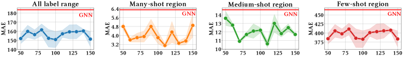
Besides molecules and polymers, Table 3 presents more results by comparing different methods on the Superpixel-Age dataset. SGIR consistently improves the model performance compared to the best baselines in different label ranges. In the entire label range, SGIR reduces the MAE (GM) relatively by +4.7% (+3.6%). The advantages mainly stem from the enhancements in the few-shot region, as demonstrated in Table 3, which shows an improvement of +4.3% and +3.1% on the MAE and GM metrics, respectively. Different from LDS, SGIR improves the model performance for the under-represented and well-represented label ranges at the same time. Table 3 showcases that the empirical advantages of SGIR could generalize across different domains.

5.3. RQ2: Ablation Studies on Framework Design

We conduct five studies and analyze the results below. Four ablation studies are (1) $\mathcal{G}_{\text{conf}}$ and $\mathcal{H}_{\text{aug}}$ for data balancing; (2) mutually enhanced iterative process; (3) choices of confidence score; and (4) quality and diversity of the label-anchored mixup. (5) The sensitivity analysis for the label interval number $C$ . Readers can refer to the appendix for complete results.

5.3.1. Effect of balancing data with different components in $\mathcal{G}_{\text{conf}}$ and $\mathcal{H}_{\text{aug}}$

Studies on molecule regression tasks in Table 5 present how SGIR improves the initial supervised performance to the most advanced semi-supervised performance step by step. In the first line for each dataset, we use only imbalanced training data $\mathcal{G}_{\text{conf}}$ to train the regression model and observe that the model performs badly in the few-shot region. The fourth line for each dataset combines the use of regression confidence $\sigma$ and the reverse sampling $p$ to produce $\mathcal{G}_{\text{conf}}$ . It improves the MAE performance in the few-shot region relatively by +11.2%, +3.2%, and +15.9% on the Mol-Lipo, Mol-ESOL, and Mol-FreeSolv datasets, respectively. The label-anchored mixup algorithm produces the augmented graph representations $\mathcal{H}_{\text{aug}}$ for the under-represented label ranges. By applying $\mathcal{H}_{\text{aug}}$ with $\mathcal{G}_{\text{conf}}$ , the last line continues improving the MAE performance in the few-shot region (compared to the third line) relatively by +3.3%, +1.3%, and +6.5% on the Mol-Lipo, Mol-ESOL, and Mol-FreeSolv datasets, respectively. Because the use of $\mathcal{H}_{\text{aug}}$ provides a chance to lead the label distributions of training data closer to a perfect balance. Specifically, the effect of semi-supervised pseudo-labeling, or $\mathcal{G}_{\text{conf}}$ , comes from the regression confidence $\sigma$ and reverse sampling rate $p$ . Results on Mol-ESOL and Mol-FreeSolv show that without the confidence $\sigma$ (the second line), reverse sampling was useless due to heavy label noise. Results on all molecule datasets indicate that without the reverse sampling rate $p$ (the first line), the improvement to few-shot region by pseudo-labels was limited.

5.3.2. Effect of iterative self-training

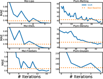
Figure 4 confirms that model learning and balanced training data mutually enhance each other in SGIR. Because we find that the model performance gradually approximates and outperforms the best baseline in the entire label range, as well as the few-shot region, after multiple iterations. It also indicates that the quality of the training data is steadily improved over iterations. Especially for the under-represented label ranges.

5.3.3. Effect of regression confidence measurements

Table 5 shows that compared to existing methods that could define regression confidence, the measurement we define and use, GRation, is the best option for evaluating the quality of pseudo-labels in graph regression tasks. Because GRation uses various environments subgraphs, which provide diverse perturbations for robust graph learning (Liu et al., 2022). We also observe that Dropout can be a good alternative of GRation. Dropout has extensive assessments (Gal and Ghahramani, 2016) and makes it possible for SGIR to be extended to regression tasks for other data types such as images and texts.

5.3.4. Effect of label-anchored mixup augmentation

We implement $\mathbf{z}_{i}$ using $\mathcal{G}_{\text{imb}}$ to improve the augmentation quality and $\mathcal{G}_{\text{imb}}\cup\mathcal{G}_{\text{unlbl}}$ to improve the diversity. Table 6 presents extensive empirical studies to support our idea. It shows that when many noisy representation vectors from unlabeled graphs are included in the interval center $\mathbf{z}_{i}$ , the quality of augmented examples is relatively low, which degrades the model performance in different label ranges. On the other hand, the representations of unlabeled graphs improve the diversity of the augmented examples when we assign low mixup weights to them as in Eq. 5. Considering both quality and diversity, the effectiveness of the algorithm is further demonstrated in Table 5 by significantly reducing the errors for rare labels. From the fifth line of each dataset in Table 5, we find that it is also promising to directly use the label-anchored mixup augmentation (as $\mathcal{G}_{\text{imb}}\cup\mathcal{H}_{\text{aug}}$ ) for data balancing. Although its performance may be inferior to the performance using $\mathcal{G}_{\text{imb}}\cup\mathcal{G}_{\text{conf}}$ (as the third line of each dataset in Table 5), the potential of the label-anchored mixup algorithm could be further enhanced by improving the quality of the augmented examples to close the gap with real molecular graphs.

5.3.5. Sensitivity analysis for the label interval number $C$

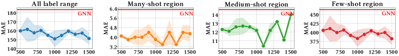
We find the best values of $C$ in main experiments using the validation set for pseudo-labeling and label-anchored mixup. We suggest setting the number $C$ to approximately 100 for pseudo-labeling and around 1,000 for label-anchored mixup. Specifically, sensitivity analysis is conducted on the Plym-Oxygen dataset to analyze the effect of the number $C$ . Results are presented in Figure 5. We observe that SGIR is robust to a wide range of choices for the number of intervals.

6. Conclusions

In this work, we explored a novel graph imbalanced regression task and improved semi-supervised learning on it. We proposed a self-training framework to gradually reduce the model bias of data imbalance through multiple iterations. In each iteration, we selected more high-quality pseudo-labels for rare label values and continued augmenting training data to approximate the perfectly balanced label distribution. Experiments demonstrated the effectiveness and reasonable design of the proposed framework, especially on material science.

Acknowledgements.

This work was supported in part by NSF IIS-2142827, IIS-2146761, and ONR N00014-22-1-2507.

References

(1)
Achanta et al. (2012) Radhakrishna Achanta, Appu Shaji, Kevin Smith, Aurelien Lucchi, Pascal Fua, and Sabine Süsstrunk. 2012. SLIC superpixels compared to state-of-the-art superpixel methods. IEEE transactions on pattern analysis and machine intelligence 34, 11 (2012), 2274–2282.
Amini et al. (2020) Alexander Amini, Wilko Schwarting, Ava Soleimany, and Daniela Rus. 2020. Deep evidential regression. Advances in Neural Information Processing Systems 33 (2020), 14927–14937.
Bartlett and Mendelson (2002) Peter L Bartlett and Shahar Mendelson. 2002. Rademacher and Gaussian complexities: Risk bounds and structural results. Journal of Machine Learning Research 3, Nov (2002), 463–482.
Berthelot et al. (2019) David Berthelot, Nicholas Carlini, Ian Goodfellow, Nicolas Papernot, Avital Oliver, and Colin A Raffel. 2019. Mixmatch: A holistic approach to semi-supervised learning. Advances in Neural Information Processing Systems 32 (2019).
Berthelot et al. (2022) David Berthelot, Rebecca Roelofs, Kihyuk Sohn, Nicholas Carlini, and Alex Kurakin. 2022. Adamatch: A unified approach to semi-supervised learning and domain adaptation. International Conference on Learning Representations (2022).
Branco et al. (2017) Paula Branco, Luís Torgo, and Rita P Ribeiro. 2017. SMOGN: a pre-processing approach for imbalanced regression. In First international workshop on learning with imbalanced domains: Theory and applications. PMLR, 36–50.
Cao et al. (2019) Kaidi Cao, Colin Wei, Adrien Gaidon, Nikos Arechiga, and Tengyu Ma. 2019. Learning imbalanced datasets with label-distribution-aware margin loss. Advances in neural information processing systems 32 (2019).
Carratino et al. (2020) Luigi Carratino, Moustapha Cissé, Rodolphe Jenatton, and Jean-Philippe Vert. 2020. On mixup regularization. arXiv preprint arXiv:2006.06049 (2020).
Chawla et al. (2002) Nitesh V Chawla, Kevin W Bowyer, Lawrence O Hall, and W Philip Kegelmeyer. 2002. SMOTE: synthetic minority over-sampling technique. Journal of artificial intelligence research 16 (2002), 321–357.
Cortes et al. (2008) Corinna Cortes, Mehryar Mohri, Michael Riley, and Afshin Rostamizadeh. 2008. Sample selection bias correction theory. In Algorithmic Learning Theory: 19th International Conference, ALT 2008, Budapest, Hungary, October 13-16, 2008. Proceedings 19. Springer, 38–53.
Cui et al. (2019) Yin Cui, Menglin Jia, Tsung-Yi Lin, Yang Song, and Serge Belongie. 2019. Class-balanced loss based on effective number of samples. In Proceedings of the IEEE/CVF conference on computer vision and pattern recognition. 9268–9277.
Gal and Ghahramani (2016) Yarin Gal and Zoubin Ghahramani. 2016. Dropout as a bayesian approximation: Representing model uncertainty in deep learning. In international conference on machine learning. PMLR, 1050–1059.
Gong et al. (2022) Yu Gong, Greg Mori, and Frederick Tung. 2022. RankSim: Ranking Similarity Regularization for Deep Imbalanced Regression. International Conference on Machine Learning (2022).
Hamilton et al. (2017) William L Hamilton, Rex Ying, and Jure Leskovec. 2017. Inductive representation learning on large graphs. In Proceedings of the 31st International Conference on Neural Information Processing Systems. 1025–1035.
Han et al. (2022) Xiaotian Han, Zhimeng Jiang, Ninghao Liu, and Xia Hu. 2022. G-Mixup: Graph Data Augmentation for Graph Classification. arXiv preprint arXiv:2202.07179 (2022).
He et al. (2021) Ju He, Adam Kortylewski, Shaokang Yang, Shuai Liu, Cheng Yang, Changhu Wang, and Alan Yuille. 2021. Rethinking Re-Sampling in Imbalanced Semi-Supervised Learning. arXiv preprint arXiv:2106.00209 (2021).
Hu et al. (2022) Xinting Hu, Yulei Niu, Chunyan Miao, Xian-Sheng Hua, and Hanwang Zhang. 2022. On Non-Random Missing Labels in Semi-Supervised Learning. In International Conference on Learning Representations.
Jean et al. (2018) Neal Jean, Sang Michael Xie, and Stefano Ermon. 2018. Semi-supervised deep kernel learning: Regression with unlabeled data by minimizing predictive variance. Advances in Neural Information Processing Systems 31 (2018).
Kakade et al. (2008) Sham M Kakade, Karthik Sridharan, and Ambuj Tewari. 2008. On the complexity of linear prediction: Risk bounds, margin bounds, and regularization. Advances in neural information processing systems 21 (2008).
Kim et al. (2020) Jaehyung Kim, Youngbum Hur, Sejun Park, Eunho Yang, Sung Ju Hwang, and Jinwoo Shin. 2020. Distribution aligning refinery of pseudo-label for imbalanced semi-supervised learning. Advances in Neural Information Processing Systems 33 (2020), 14567–14579.
Kipf and Welling (2017) Thomas N Kipf and Max Welling. 2017. Semi-supervised classification with graph convolutional networks. In International Conference on Learning Representations.
Knyazev et al. (2019) Boris Knyazev, Graham W Taylor, and Mohamed Amer. 2019. Understanding attention and generalization in graph neural networks. Advances in neural information processing systems 32 (2019).
Lin et al. (2017) Tsung-Yi Lin, Priya Goyal, Ross Girshick, Kaiming He, and Piotr Dollár. 2017. Focal loss for dense object detection. In Proceedings of the IEEE international conference on computer vision. 2980–2988.
Liu et al. (2023a) Gang Liu, Eric Inae, Tong Zhao, Jiaxin Xu, Tengfei Luo, and Meng Jiang. 2023a. Data-Centric Learning from Unlabeled Graphs with Diffusion Model. arXiv preprint arXiv:2303.10108 (2023).
Liu et al. (2022) Gang Liu, Tong Zhao, Jiaxin Xu, Tengfei Luo, and Meng Jiang. 2022. Graph Rationalization with Environment-based Augmentations. In Proceedings of the 28th ACM SIGKDD International Conference on Knowledge Discovery & Data Mining.
Liu et al. (2023b) Zixuan Liu, Ziqiao Wang, Hongyu Guo, and Yongyi Mao. 2023b. Over-Training with Mixup May Hurt Generalization. In The Eleventh International Conference on Learning Representations. https://openreview.net/forum?id=JmkjrlVE-DG
Ma and Luo (2020) Ruimin Ma and Tengfei Luo. 2020. PI1M: a benchmark database for polymer informatics. Journal of Chemical Information and Modeling 60, 10 (2020), 4684–4690.
McLachlan (1975) Geoffrey J McLachlan. 1975. Iterative reclassification procedure for constructing an asymptotically optimal rule of allocation in discriminant analysis. J. Amer. Statist. Assoc. 70, 350 (1975), 365–369.
Mendez et al. (2019) David Mendez, Anna Gaulton, A Patrícia Bento, Jon Chambers, Marleen De Veij, Eloy Félix, María Paula Magariños, Juan F Mosquera, Prudence Mutowo, Michał Nowotka, et al. 2019. ChEMBL: towards direct deposition of bioassay data. Nucleic acids research 47, D1 (2019), D930–D940.
Menon et al. (2021) Aditya Krishna Menon, Sadeep Jayasumana, Ankit Singh Rawat, Himanshu Jain, Andreas Veit, and Sanjiv Kumar. 2021. Long-tail learning via logit adjustment. In International Conference on Learning Representations. https://openreview.net/forum?id=37nvvqkCo5
Moschoglou et al. (2017) Stylianos Moschoglou, Athanasios Papaioannou, Christos Sagonas, Jiankang Deng, Irene Kotsia, and Stefanos Zafeiriou. 2017. Agedb: the first manually collected, in-the-wild age database. In proceedings of the IEEE conference on computer vision and pattern recognition workshops. 51–59.
Oh et al. (2022) Youngtaek Oh, Dong-Jin Kim, and In So Kweon. 2022. Distribution-aware semantics-oriented pseudo-label for imbalanced semi-supervised learning. In Proceedings of the IEEE/CVF Conference on Computer Vision and Pattern Recognition.
Otsuka et al. (2011) Shingo Otsuka, Isao Kuwajima, Junko Hosoya, Yibin Xu, and Masayoshi Yamazaki. 2011. PoLyInfo: Polymer database for polymeric materials design. In 2011 International Conference on Emerging Intelligent Data and Web Technologies. IEEE, 22–29.
Ramakrishnan et al. (2014) Raghunathan Ramakrishnan, Pavlo O Dral, Matthias Rupp, and O Anatole Von Lilienfeld. 2014. Quantum chemistry structures and properties of 134 kilo molecules. Scientific data 1, 1 (2014), 1–7.
Ren et al. (2022) Jiawei Ren, Mingyuan Zhang, Cunjun Yu, and Ziwei Liu. 2022. Balanced MSE for Imbalanced Visual Regression. In Proceedings of the IEEE/CVF Conference on Computer Vision and Pattern Recognition.
Rong et al. (2019) Yu Rong, Wenbing Huang, Tingyang Xu, and Junzhou Huang. 2019. DropEdge: Towards Deep Graph Convolutional Networks on Node Classification. arXiv preprint arXiv:1907.10903 (2019).
Sohn et al. (2020) Kihyuk Sohn, David Berthelot, Nicholas Carlini, Zizhao Zhang, Han Zhang, Colin A Raffel, Ekin Dogus Cubuk, Alexey Kurakin, and Chun-Liang Li. 2020. Fixmatch: Simplifying semi-supervised learning with consistency and confidence. Advances in Neural Information Processing Systems 33 (2020), 596–608.
Sugiyama and Storkey (2006) Masashi Sugiyama and Amos J Storkey. 2006. Mixture regression for covariate shift. Advances in neural information processing systems 19 (2006).
Sun et al. (2016) Baochen Sun, Jiashi Feng, and Kate Saenko. 2016. Return of frustratingly easy domain adaptation. In Proceedings of the AAAI conference on artificial intelligence, Vol. 30.
Sun et al. (2020) Fan-Yun Sun, Jordon Hoffman, Vikas Verma, and Jian Tang. 2020. InfoGraph: Unsupervised and Semi-supervised Graph-Level Representation Learning via Mutual Information Maximization. In International Conference on Learning Representations.
Tagasovska and Lopez-Paz (2019) Natasa Tagasovska and David Lopez-Paz. 2019. Single-model uncertainties for deep learning. Advances in Neural Information Processing Systems 32 (2019).
Thornton et al. (2012) A Thornton, L Robeson, B Freeman, and D Uhlmann. 2012. Polymer Gas Separation Membrane Database.
Tian et al. (2020) Junjiao Tian, Yen-Cheng Liu, Nathaniel Glaser, Yen-Chang Hsu, and Zsolt Kira. 2020. Posterior re-calibration for imbalanced datasets. Advances in Neural Information Processing Systems 33 (2020), 8101–8113.
Veličković et al. (2018) Petar Veličković, Guillem Cucurull, Arantxa Casanova, Adriana Romero, Pietro Liò, and Yoshua Bengio. 2018. Graph Attention Networks. In International Conference on Learning Representations.
Verma et al. (2019) Vikas Verma, Alex Lamb, Christopher Beckham, Amir Najafi, Ioannis Mitliagkas, David Lopez-Paz, and Yoshua Bengio. 2019. Manifold mixup: Better representations by interpolating hidden states. In International Conference on Machine Learning. PMLR, 6438–6447.
Wang et al. (2021) Yiwei Wang, Wei Wang, Yuxuan Liang, Yujun Cai, and Bryan Hooi. 2021. Mixup for node and graph classification. In Proceedings of the Web Conference 2021. 3663–3674.
Wei et al. (2021) Chen Wei, Kihyuk Sohn, Clayton Mellina, Alan Yuille, and Fan Yang. 2021. CREST: A class-rebalancing self-training framework for imbalanced semi-supervised learning. In Proceedings of the IEEE/CVF Conference on Computer Vision and Pattern Recognition. 10857–10866.
Wu et al. (2022) Ying-Xin Wu, Xiang Wang, An Zhang, Xiangnan He, and Tat seng Chua. 2022. Discovering Invariant Rationales for Graph Neural Networks. In ICLR.
Wu et al. (2018) Zhenqin Wu, Bharath Ramsundar, Evan N Feinberg, Joseph Gomes, Caleb Geniesse, Aneesh S Pappu, Karl Leswing, and Vijay Pande. 2018. MoleculeNet: a benchmark for molecular machine learning. Chemical science 9, 2 (2018), 513–530.
Xie et al. (2020) Qizhe Xie, Minh-Thang Luong, Eduard Hovy, and Quoc V Le. 2020. Self-training with noisy student improves imagenet classification. In Proceedings of the IEEE/CVF conference on computer vision and pattern recognition. 10687–10698.
Xu et al. (2019) Keyulu Xu, Weihua Hu, Jure Leskovec, and Stefanie Jegelka. 2019. How Powerful are Graph Neural Networks?. In International Conference on Learning Representations. https://openreview.net/forum?id=ryGs6iA5Km
Yang et al. (2021) Yuzhe Yang, Kaiwen Zha, Yingcong Chen, Hao Wang, and Dina Katabi. 2021. Delving into deep imbalanced regression. In International Conference on Machine Learning. PMLR, 11842–11851.
Yao et al. (2022) Huaxiu Yao, Yiping Wang, Linjun Zhang, James Y Zou, and Chelsea Finn. 2022. C-mixup: Improving generalization in regression. Advances in Neural Information Processing Systems 35 (2022), 3361–3376.
Yuan et al. (2021) Qi Yuan, Mariagiulia Longo, Aaron W Thornton, Neil B McKeown, Bibiana Comesana-Gandara, Johannes C Jansen, and Kim E Jelfs. 2021. Imputation of missing gas permeability data for polymer membranes using machine learning. Journal of Membrane Science 627 (2021), 119207.
Zhang et al. (2021) Linjun Zhang, Zhun Deng, Kenji Kawaguchi, Amirata Ghorbani, and James Zou. 2021. How Does Mixup Help With Robustness and Generalization?. In International Conference on Learning Representations. https://openreview.net/forum?id=8yKEo06dKNo
Zhang et al. (2023) Yifan Zhang, Bingyi Kang, Bryan Hooi, Shuicheng Yan, and Jiashi Feng. 2023. Deep long-tailed learning: A survey. IEEE Transactions on Pattern Analysis and Machine Intelligence (2023).
Zhao et al. (2021a) Tong Zhao, Tianwen Jiang, Neil Shah, and Meng Jiang. 2021a. A synergistic approach for graph anomaly detection with pattern mining and feature learning. IEEE Transactions on Neural Networks and Learning Systems 33, 6 (2021), 2393–2405.
Zhao et al. (2022a) Tong Zhao, Wei Jin, Yozen Liu, Yingheng Wang, Gang Liu, Stephan Günneman, Neil Shah, and Meng Jiang. 2022a. Graph Data Augmentation for Graph Machine Learning: A Survey. arXiv preprint arXiv:2202.08871 (2022).
Zhao et al. (2022b) Tong Zhao, Gang Liu, Daheng Wang, Wenhao Yu, and Meng Jiang. 2022b. Learning from Counterfactual Links for Link Prediction. In International Conference on Machine Learning. PMLR, 26911–26926.
Zhao et al. (2021b) Tong Zhao, Yozen Liu, Leonardo Neves, Oliver Woodford, Meng Jiang, and Neil Shah. 2021b. Data Augmentation for Graph Neural Networks. In Proceedings of the AAAI Conference on Artificial Intelligence, Vol. 35. 11015–11023.

Table 7. Comparing SGIR with related methods on research problem settings.

	Is Semi-supervised	Learning	Addressing	Solving
	method?	Graph data?	Imbalance?	Regression?
(Otherwise, assuming:)	(Supervised)	(Non-graph)	(Balance)	(Classification)
DARP (Kim et al., 2020)	✓		✓
DASO (Oh et al., 2022)	✓		✓
Bi-Sampling (He et al., 2021)	✓		✓
CADR (Hu et al., 2022)	✓		✓
CReST (Wei et al., 2021)	✓		✓
LDS (Yang et al., 2021)			✓	✓
BMSE (Ren et al., 2022)			✓	✓
RankSim (Gong et al., 2022)			✓	✓
SSDKL (Jean et al., 2018)	✓			✓
InfoGraph (Sun et al., 2020)	✓	✓		✓
SGIR (Ours)	✓	✓	✓	✓

Appendix A Further Related Work

A.1. A Systematic Comparison with Related Methods

We compare SGIR with a line of related work on four important settings of research problem in Table 7. From the table we find that existing work mostly focused on solving imbalance problems in semi-supervised classification tasks with categorical labels and non-graph data. There lacks an exploration of research on semi-supervised learning and imbalance learning for graph regression.

A.2. Sampling Strategy in Self-training

To the best of our knowledge, reverse sampling is one of the most suitable sampling strategies to address class imbalance issues in self-training (Wei et al., 2021). Compared to other strategies like random sampling or mean sampling (He et al., 2021), reverse sampling is also the most suitable one for graph imbalanced regression. This is because reverse sampling compensates for the label imbalance and enriches training examples. Other strategies cannot make the training data more balanced. They would lead the prediction model to be still biased to the majority of data. More complex sampling strategies that combine reverse sampling, mean sampling, and random sampling would be a promising direction for future work.

Appendix B Proofs of Theoretical Motivations

We rely on two theorems to derive theorem 4.1.

B.1. Existing Theorems

Given a classifier $f$ from the function class $\mathcal{F}$ , an input example $x$ from the feature space $\mathcal{X}$ and its label $y$ .

Theorem B.1 (from (Bartlett and Mendelson, 2002; Kakade et al., 2008)).

Assume the expected loss on examples is $\mathcal{E}[f]$ and the corresponding empirical loss $\hat{\mathcal{E}[f]}$ . Assume the loss is Lipschitz with Lipschitz constant $L_{e}$ . And it is bounded by $c_{0}$ . For any $\delta>0$ and with probability at least $1-\delta$ simultaneously for all $f\in\mathcal{F}$ we have that

(10)

\mathcal{E}[f]\leq\hat{\mathcal{E}}[f]+2L_{e}\mathcal{R}_{n}(\mathcal{F})+c_{0}\sqrt{\frac{\log(1/\delta)}{2n}},

where $n$ is the number of example and $\hat{\mathcal{R}}_{n}(\mathcal{F})$ is the Rademacher complexity measurement of the hypothesis class $\mathcal{F}$ .

Theorem B.2 (from (Kakade et al., 2008)).

Applying theorem B.1 and considering the fraction of data having $\gamma$ -margin mistakes, or $K_{\gamma}[f]:=\frac{|i:y_{i}f(x_{i})<\gamma|}{n}$ . Assume $\forall f\in\mathcal{F}$ we have $\operatorname{sup}_{x\in\mathcal{X}}|f(x)|\leq c_{1}$ . Then, with probability at least $1-\delta$ over the example, for all margins $\gamma>0$ and all $f\in\mathcal{F}$ we have,

(11)		$\displaystyle\mathcal{E}[f]$	$\displaystyle\leq K_{\gamma}[f]+4\frac{\mathcal{R}_{n}(\mathcal{F})}{\gamma}+\sqrt{\frac{2\log\left(\log_{2}(4c_{1}/\gamma)\right)+\log(1/\delta)}{2n}},$
(12)			$\displaystyle\leq K_{\gamma}[f]+4\frac{\mathcal{R}_{n}(\mathcal{F})}{\gamma}+\sqrt{\frac{\log\left(\log_{2}\frac{4c_{1}}{\gamma}\right)}{n}}+\sqrt{\frac{\log(1/\delta)}{2n}}.$

B.2. Proof of theorem 4.1

In our work, we use the regression function $f$ to predict the label value. We calculate the reciprocal of the distance between the predicted label and interval centers as unnormalized probabilities of the graph $S_{[b_{i},b_{i+1})}(G)$ being assigned to the interval $[b_{i},b_{i+1}),i\in\{1,2,\dots,C\}$ . Given a hard margin $\gamma$ , we use $\mathcal{E}_{\gamma,[b_{i},b_{i+1})}[f]$ to denote the hard margin loss for examples in the interval $[b_{i},b_{i+1})$ :

(13)

\mathcal{E}_{\gamma,[b_{i},b_{i+1})}[f]=\underset{G\sim\mathcal{P}_{[b_{i},b_{i+1})}}{\operatorname{Pr}}\left[S_{[b_{i},b_{i+1})}(G)<\max_{j\neq i}S_{[b_{j},b_{j+1})}(G)+\gamma\right].

We assume its empirical variant is $\hat{\mathcal{E}}_{\gamma,[b_{i},b_{i+1})}[f]$ . The empirical Rademacher complexity $\hat{\mathcal{R}}_{(b_{i},b_{i+1}]}(\mathcal{F})$ is used as the complexity measurement $\textup{C}(\mathcal{F})$ for the hypothesis class $\mathcal{F}$ . With a vector $\sigma$ of i.i.d. uniform $\{-1,+1\}$ bits, we have

(14)		$\displaystyle\hat{\mathcal{R}}_{(b_{i},b_{i+1}]}(\mathcal{F})=$
(15)		$\displaystyle\frac{1}{n_{(b_{i},b_{i+1}]}}\mathbb{E}_{\sigma}\left[\sup_{f\in\mathcal{F}}\sum_{G_{i}\in[b_{i},b_{i+1})}\sigma_{i}\left[S_{[b_{i},b_{i+1})}\left(G_{i}\right)-\max_{j\neq i}S_{[b_{j},b_{j+1})}\left(G_{i}\right)\right]\right]$

As any $G_{i}$ in the interval ${(b_{i},b_{i+1}]}$ is an i.i.d. sample from the distribution $\mathcal{P}_{[b_{i},b_{i+1})}$ , we directly apply the standard margin-based generalization bound theorem B.2 (Kakade et al., 2008): with probability $1-\delta$ , for all choices of $\gamma_{{}_{[b_{i},b_{i+1})}}>0$ and $f\in\mathcal{F}$ ,

(16)	$\displaystyle\mathcal{E}_{[b_{i},b_{i+1})}$	$\displaystyle\leq\hat{\mathcal{E}}_{\gamma,[b_{i},b_{i+1})}[f]+4\frac{\hat{\mathcal{R}}_{(b_{i},b_{i+1}]}(\mathcal{F})}{\gamma_{{}_{[b_{i},b_{i+1})}}}$
	$\displaystyle\quad\quad\quad\quad+\sqrt{\frac{2\log\left(\log_{2}(\frac{4c_{1}}{\gamma_{{}_{[b_{i},b_{i+1})}}})\right)+\log(1/\delta)}{2n_{[b_{i},b_{i+1})}}},$
(17)		$\displaystyle\leq\hat{\mathcal{E}}_{\gamma,[b_{i},b_{i+1})}[f]+\frac{1}{\gamma_{{}_{[b_{i},b_{i+1})}}}\sqrt{\frac{\textup{C}(\mathcal{F})}{n_{[b_{i},b_{i+1})}}}$
	$\displaystyle\quad\quad\quad\quad+\sqrt{\frac{2\log\left(\log_{2}(\frac{4c_{1}}{\gamma_{{}_{[b_{i},b_{i+1})}}})\right)\log(1/\delta)}{2n_{[b_{i},b_{i+1})}}},$
(18)		$\displaystyle\lessapprox\frac{1}{\gamma_{{}_{[b_{i},b_{i+1})}}}\sqrt{\frac{\textup{C}(\mathcal{F})}{n_{[b_{i},b_{i+1})}}}+\sqrt{\frac{\log\log_{2}(1/\gamma_{{}_{[b_{i},b_{i+1})}})+\log(1/\delta)}{{2n_{[b_{i},b_{i+1})}}}}.$

We derive Eq. 17 from Eq. 16 because the Rademacher complexity $\hat{\mathcal{R}}_{(b_{i},b_{i+1}]}(\mathcal{F})$ typically scales as $\sqrt{\frac{\textup{C}(\mathcal{F})}{n_{(b_{i},b_{i+1}]}}}$ for some complexity measurement $\textup{C}(\mathcal{F})$ (Cao et al., 2019). We derive Eq. 18 from Eq. 17 by ignoring constant factors (Cao et al., 2019). Since the overall performance $\mathcal{E}_{\textup{bal}}[f]$ is calculated over all intervals, we get it as $\mathcal{E}_{\textup{bal}}[f]=\frac{1}{C}\sum_{i=1}^{C}\mathcal{E}_{[b_{i},b_{i+1})}$ .

B.3. Discussions

Existing work on the theoretical analysis of mixup (Liu et al., 2023b; Carratino et al., 2020; Zhang et al., 2021) mainly focused on image classification and cannot guarantee that the augmented graph examples are i.i.d sampled from the conditional distribution $\mathcal{P}_{[b_{i},b_{i+1}]}$ for a specific interval $[b_{i},b_{i+1}]$ . While a recent work proposed the C-mixup (Yao et al., 2022) to sample closer pairs of examples with higher probability for regression tasks, it did not fit our theoretical motivation to address the label imbalance issue: with C-mixup, the pairs in the over-represented label ranges have a higher probability to be sampled than the under-represented ones. Compared to these theories and methods for the mixup algorithm, our label-anchored mixup allows direct application to imbalanced regression tasks without compromising the assumption in our theoretical motivation. This is because we use the augmented virtual examples $\mathcal{H}_{\text{aug}}$ based on the label anchor within intervals $[b_{i},b_{i+1}]$ . Augmented examples are independently created with Eq. 5. Since the interval centers could be mixed with any other real graphs from $\mathcal{G}_{\text{imb}}\cup\mathcal{G}_{\text{conf}}$ , any value in the interval space could be sampled. Besides, it is reasonable to use the distribution of the entire label space (from $\mathcal{G}_{\text{imb}}\cup\mathcal{G}_{\text{conf}}$ ) to approximate the distribution within the interval and assume that the conditional distribution $\mathcal{P}_{[b_{i},b_{i+1}]}$ does not change.

We build the theoretical principle for imbalanced regression with intervals to connect with existing theoretical principles for classification. Future theoretical work on imbalanced regression can leverage the advantages of using mixture regressor models (Sugiyama and Storkey, 2006), which have been used to address covariate shift problems in regression tasks. Additionally, exploring the promising connection between domain adaptation theories and sample selection bias (Sun et al., 2016; Cortes et al., 2008) holds potential for further advancements in this field.

Appendix C Experiments

C.1. Dataset Details

We give a comprehensive introduction to our datasets used for regression tasks and splitting idea from (Yang et al., 2021; Gong et al., 2022).

Mol-Lipo

It is a dataset to predict the property of lipophilicity consisting of 4200 molecules. The lipophilicity is important for solubility and membrane permeability in drug molecules. This dataset originates from ChEMBL (Mendez et al., 2019). The property is from experimental results for the octanol/water distribution coefficient ( $\log D$ at pH 7.4).

Mol-ESOL

It is to predict the water solubility ( $\log$ solubility in mols per litre) from chemical structures consisting of 1128 small organic molecules.

Mol-FreeSolv

It is to predict the hydration free energy of molecules in water consisting of 642 molecules. The property is experimentally measured or calculated.

Plym-Melting

It is used to predict the property of melting temperature (^∘C). It is collected from PolyInfo, a web-based polymer database (Otsuka et al., 2011).

Plym-Density

It is used to predict the property of polymer density (g/cm³). It is collected from PolyInfo, a web-based polymer database (Otsuka et al., 2011).

Plym-Oxygen

It is used to predict the property of oxygen permeability (Barrer). It is created from the Membrane Society of Australasia portal consisting of experimentally measured gas permeability data (Thornton et al., 2012).

Unlabeled Data for Molecules and Polymers

The total number of unlabeled graphs for molecule and polymers is 146,129, consisting of 133,015 molecules from QM9 (Ramakrishnan et al., 2014) and 13,114 monomers (the repeated units of polymers) from (Liu et al., 2022). QM9 is a molecule dataset for stable small organic molecules consisting of atoms C, H, O, N, and F. We use it as a source of unlabeled data. We integrate four polymer regression datasets including Plym-Melting, Plym-Density, Plym-Oxygen and another one from (Liu et al., 2022) for the glass transition temperature as the other source of unlabeled data. We note that the unlabeled graphs may be slightly less than 146,129 for a polymer task on Plym-Melting, Plym-Density or Plym-Oxygen. It is because we remove the overlapping graphs for the current polymer task with the polymer unlabeled data.

Data splitting for Molecules and Polymers

We split the datasets based on the approach in previous works (Yang et al., 2021; Gong et al., 2022) motivated for two reasons. First, we want the training sets to well characterize the imbalanced label distribution as presented in the original datasets. Second, we want relatively balanced valid and test sets to fairly evaluate the model performance in different ranges of label values.

Superpixel-Age

The details of the age regression dataset are presented in Table 1 (Superpixel-Age) and Figure 3. The graph dataset Superpixel-Age is constructed from image superpixels using the algorithms from (Knyazev et al., 2019) on the image dataset AgeDB-DIR from (Moschoglou et al., 2017; Yang et al., 2021). Each face image in AgeDB-DIR has an age label from 0 to 101. We fisrt compute the SLIC superpixels for each image without losing the label-specific information (Achanta et al., 2012; Knyazev et al., 2019). Then we use the superpixels as nodes and calculate the spatial distance between superpixels to build edges for each image (Knyazev et al., 2019). Binary edges are constructed between superpixel nodes by applying a threshold on the top-5% of the smallest spatial distances. After building a graph for each image, we follow the data splitting in (Yang et al., 2021) to study the imbalanced regression problem. We randomly remove 70% labels in the training/validation/test data and use them as unlabeled graphs. Finally, the graph dataset Superpixel-Age consists of 3,619 graphs for training, 628 graphs for validation, 628 graphs for testing, and 11,613 unlabeled graphs for semi-supervised learning.

C.2. Implementation Details

We use the Graph Isomorphism Network (GIN) (Xu et al., 2019) as the GNN encoder for $f_{\theta}$ to get the graph representation and three layers of Multilayer perceptron (MLP) as the decoder to predict graph properties. The threshold $\tau$ for selecting confident predictions is determined by the value at a certain percentile of the confidence score distribution. To implement it, we set it up as a hyperparameter $\tau_{\text{pct}}$ determining the percentile value of the prediction variance (i.e., the reciprocal of confidence) of the labeled training data. In experiments, all methods are implemented on Linux with Intel Xeon Gold 6130 Processor (16 Cores @2.1Ghz), 96 GB of RAM, and a RTX 2080Ti card (11 GB RAM). For all the methods, we reports the results on the test sets using the mean (standard deviation) over 10 runs with parameters that are randomly initialized. Note that the underlying design of the graph learning model used in SGIR is GREA with a learning objective as follows. Given $(G,y)\in\mathcal{G}_{\text{imb}}\cup\mathcal{G}_{\text{conf}}$ , GREA (Liu et al., 2022) will output a vector $\mathbf{m}\in\mathbb{R}^{K}$ that indicates the probability of $K$ nodes in a graph being in the rationale subgraph. So, we could get $\mathbf{h}^{(r)}=\mathbf{1}^{\top}_{K}\cdot(\mathbf{m}\times\mathbf{H})$ and $\mathbf{h}^{(e)}=\mathbf{1}^{\top}_{K}\cdot((\mathbf{1}_{K}-\mathbf{m})\times\mathbf{H})$ , where $\mathbf{H}\in\mathbb{R}^{K\times d}$ is the node representation matrix. By this, the optimization objectives of a graph consist of

\begin{cases}&\ell_{\text{imb+conf}}=\operatorname{MAE}(f(\mathbf{h}^{(r)}),y)+\mathbb{E}_{G^{\prime}}\big{[}\operatorname{MAE}(f(\mathbf{h}+\mathbf{h}^{\prime}),y)\big{]}\\ &\quad\quad\quad+\operatorname{Var}_{G^{\prime}}\big{(}\{\operatorname{MAE}(f(\mathbf{h}+\mathbf{h}^{\prime}),y)\}\big{)},\\ \\ &\ell_{\text{regu}}=\frac{1}{K}\sum_{k=1}^{K}|\mathbf{m}_{k}|-\gamma\end{cases}

$\ell_{\text{regu}}$ regularizes the vector $\mathbf{m}$ and $\gamma\in[0,1]$ is a hyperparameter to control the expected size of $G^{(r)}$ . $G^{\prime}$ is the possible graph in the same batch that provides environment subgraphs and $\mathbf{h}^{\prime}$ is the representation vector of the environment subgraph. When combining the rationale-environment pairs to create new graph examples, the original GREA creates the same number of examples for the under-represented rationale and the well/over-represented rationale. We observe that it may make the training examples more imbalanced. Therefore, we use the reweighting technique to penalize more for the expectation term ( $\mathbb{E}_{G^{\prime}}\big{[}\operatorname{MAE}(f(\mathbf{h}+\mathbf{h}^{\prime}),y)\big{]}$ ) and variance term ( $\operatorname{Var}_{G^{\prime}}\big{(}\{\operatorname{MAE}(f(\mathbf{h}+\mathbf{h}^{\prime}),y)\}\big{)}$ ) in $\ell_{\text{imb+conf}}$ when the label is from the under-represented ranges. The weight of the expectation and variance terms for a graph with label $y$ is

w=\frac{\exp(\sum_{b=1}^{B}|y-y_{b}|/t)}{\exp(\sum_{j=1}^{B}\sum_{b=1}^{B}|y-y_{b}|/t)},

where $B$ is the batch size and $t$ is the temperature hyper-parameter.

C.3. Additional Experimental Results

Table 8. Complete results of ablation study and mixup options (MAE

\downarrow

and GM

\downarrow

) on three molecule datasets. The best mean is bolded. For the label-anchored mixup options, the first column is the source of

\textbf{z}_{i}

and the second column is the source of

\textbf{h}_{j}

			MAE $\downarrow$				GM $\downarrow$
			All	Many-shot	Med.-shot	Few-shot	All	Many-shot	Med.-shot	Few-shot
Mol-Lipo
Ablation Study	$\mathcal{G}_{\text{imb}}$		0.477(0.014)	0.378(0.030)	0.440(0.011)	0.600(0.006)	0.288(0.008)	0.236(0.015)	0.267(0.013)	0.371(0.017)
	$\mathcal{G}_{\text{imb}}\cup\mathcal{G}_{\text{conf}}$		0.442(0.012)	0.372(0.007)	0.415(0.004)	0.533(0.026)	0.267(0.013)	0.240(0.008)	0.245(0.016)	0.320(0.027)
	$\mathcal{G}_{\text{imb}}\cup\mathcal{G}_{\text{conf}}$ (w/o $\sigma$ )		0.446(0.008)	0.356(0.003)	0.407(0.011)	0.564(0.016)	0.272(0.006)	0.222(0.002)	0.244(0.008)	0.363(0.013)
	$\mathcal{G}_{\text{imb}}\cup\mathcal{G}_{\text{conf}}$ (w/o $p$ )		0.448(0.006)	0.371(0.004)	0.421(0.012)	0.543(0.016)	0.270(0.002)	0.228(0.009)	0.255(0.008)	0.333(0.015)
	$\mathcal{G}_{\text{imb}}\cup\mathcal{H}_{\text{aug}}$		0.456(0.007)	0.372(0.014)	0.436(0.010)	0.549(0.005)	0.278(0.013)	0.235(0.019)	0.265(0.014)	0.338(0.006)
	$\mathcal{G}_{\text{imb}}\cup\mathcal{G}_{\text{conf}}\cup\mathcal{H}_{\text{aug}}$		0.432(0.012)	0.357(0.019)	0.413(0.017)	0.515(0.020)	0.264(0.013)	0.224(0.016)	0.256(0.017)	0.314(0.015)
$\textbf{z}_{i}$ and $\textbf{h}_{j}$ options in Mixup	$\mathcal{G}_{\text{imb}}$	$\mathcal{G}_{\text{imb}}$	0.439(0.004)	0.361(0.010)	0.419(0.013)	0.529(0.022)	0.267(0.005)	0.231(0.015)	0.256(0.010)	0.318(0.020)
		$\mathcal{G}_{\text{imb}}\cup\mathcal{G}_{\text{conf}}$	0.447(0.015)	0.359(0.004)	0.423(0.016)	0.549(0.033)	0.274(0.017)	0.221(0.007)	0.264(0.020)	0.344(0.031)
		$\mathcal{G}_{\text{imb}}\cup\mathcal{G}_{\text{unlbl}}$	0.432(0.012)	0.357(0.019)	0.413(0.017)	0.515(0.020)	0.264(0.013)	0.224(0.016)	0.256(0.017)	0.314(0.015)
	$\mathcal{G}_{\text{imb}}\cup\mathcal{G}_{\text{conf}}$	$\mathcal{G}_{\text{imb}}$	0.448(0.012)	0.367(0.008)	0.423(0.008)	0.544(0.028)	0.270(0.013)	0.230(0.013)	0.257(0.014)	0.328(0.025)
		$\mathcal{G}_{\text{imb}}\cup\mathcal{G}_{\text{conf}}$	0.445(0.007)	0.364(0.008)	0.418(0.010)	0.542(0.012)	0.271(0.009)	0.227(0.011)	0.256(0.011)	0.337(0.016)
		$\mathcal{G}_{\text{imb}}\cup\mathcal{G}_{\text{unlbl}}$	0.449(0.021)	0.360(0.023)	0.416(0.016)	0.560(0.039)	0.270(0.019)	0.223(0.017)	0.255(0.019)	0.340(0.032)
	$\mathcal{G}_{\text{imb}}\cup\mathcal{G}_{\text{unlbl}}$	$\mathcal{G}_{\text{imb}}$	0.446(0.007)	0.367(0.009)	0.415(0.011)	0.546(0.011)	0.268(0.006)	0.228(0.008)	0.248(0.005)	0.336(0.012)
		$\mathcal{G}_{\text{imb}}\cup\mathcal{G}_{\text{conf}}$	0.446(0.011)	0.368(0.011)	0.421(0.012)	0.539(0.024)	0.270(0.004)	0.233(0.010)	0.249(0.009)	0.334(0.017)
		$\mathcal{G}_{\text{imb}}\cup\mathcal{G}_{\text{unlbl}}$	0.451(0.007)	0.371(0.012)	0.425(0.008)	0.547(0.015)	0.273(0.008)	0.222(0.007)	0.260(0.012)	0.344(0.014)
Mol-ESOL
Ablation Study	$\mathcal{G}_{\text{imb}}$		0.477(0.027)	0.375(0.014)	0.432(0.042)	0.637(0.042)	0.273(0.024)	0.215(0.023)	0.248(0.043)	0.401(0.039)
	$\mathcal{G}_{\text{imb}}\cup\mathcal{G}_{\text{conf}}$		0.468(0.007)	0.379(0.012)	0.425(0.013)	0.612(0.028)	0.263(0.009)	0.219(0.007)	0.236(0.017)	0.366(0.020)
	$\mathcal{G}_{\text{imb}}\cup\mathcal{G}_{\text{conf}}$ (w/o $\sigma$ )		0.480(0.017)	0.380(0.035)	0.440(0.017)	0.630(0.020)	0.269(0.016)	0.219(0.028)	0.249(0.024)	0.368(0.017)
	$\mathcal{G}_{\text{imb}}\cup\mathcal{G}_{\text{conf}}$ (w/o $p$ )		0.475(0.014)	0.369(0.014)	0.446(0.017)	0.618(0.039)	0.267(0.012)	0.210(0.013)	0.251(0.017)	0.372(0.050)
	$\mathcal{G}_{\text{imb}}\cup\mathcal{H}_{\text{aug}}$		0.474(0.010)	0.353(0.018)	0.450(0.009)	0.623(0.027)	0.272(0.004)	0.202(0.012)	0.257(0.011)	0.397(0.034)
	$\mathcal{G}_{\text{imb}}\cup\mathcal{G}_{\text{conf}}\cup\mathcal{H}_{\text{aug}}$		0.457(0.015)	0.370(0.022)	0.411(0.011)	0.604(0.024)	0.263(0.016)	0.226(0.021)	0.240(0.015)	0.347(0.030)
$\textbf{z}_{i}$ and $\textbf{h}_{j}$ options in Mixup	$\mathcal{G}_{\text{imb}}$	$\mathcal{G}_{\text{imb}}$	0.466(0.009)	0.374(0.023)	0.430(0.010)	0.604(0.032)	0.266(0.010)	0.214(0.027)	0.242(0.018)	0.379(0.016)
		$\mathcal{G}_{\text{imb}}\cup\mathcal{G}_{\text{conf}}$	0.460(0.016)	0.368(0.026)	0.420(0.018)	0.605(0.026)	0.268(0.017)	0.215(0.023)	0.252(0.022)	0.362(0.016)
		$\mathcal{G}_{\text{imb}}\cup\mathcal{G}_{\text{unlbl}}$	0.457(0.015)	0.370(0.022)	0.411(0.011)	0.604(0.024)	0.263(0.016)	0.226(0.021)	0.240(0.015)	0.347(0.030)
	$\mathcal{G}_{\text{imb}}\cup\mathcal{G}_{\text{conf}}$	$\mathcal{G}_{\text{imb}}$	0.469(0.017)	0.369(0.025)	0.432(0.020)	0.615(0.037)	0.260(0.014)	0.204(0.028)	0.248(0.013)	0.358(0.048)
		$\mathcal{G}_{\text{imb}}\cup\mathcal{G}_{\text{conf}}$	0.466(0.003)	0.376(0.014)	0.425(0.011)	0.610(0.013)	0.261(0.004)	0.204(0.005)	0.242(0.013)	0.370(0.013)
		$\mathcal{G}_{\text{imb}}\cup\mathcal{G}_{\text{unlbl}}$	0.461(0.010)	0.366(0.025)	0.424(0.020)	0.604(0.026)	0.264(0.015)	0.219(0.027)	0.244(0.017)	0.354(0.036)
	$\mathcal{G}_{\text{imb}}\cup\mathcal{G}_{\text{unlbl}}$	$\mathcal{G}_{\text{imb}}$	0.472(0.009)	0.369(0.022)	0.435(0.012)	0.623(0.025)	0.266(0.005)	0.202(0.015)	0.257(0.012)	0.366(0.016)
		$\mathcal{G}_{\text{imb}}\cup\mathcal{G}_{\text{conf}}$	0.476(0.013)	0.387(0.027)	0.426(0.013)	0.630(0.042)	0.271(0.017)	0.211(0.018)	0.253(0.022)	0.382(0.040)
		$\mathcal{G}_{\text{imb}}\cup\mathcal{G}_{\text{unlbl}}$	0.479(0.026)	0.368(0.012)	0.448(0.033)	0.629(0.047)	0.269(0.016)	0.210(0.010)	0.253(0.023)	0.373(0.033)
Mol-FreeSolv
Ablation Study	$\mathcal{G}_{\text{imb}}$		0.619(0.019)	0.525(0.022)	0.590(0.035)	1.000(0.072)	0.325(0.040)	0.289(0.006)	0.316(0.062)	0.521(0.084)
	$\mathcal{G}_{\text{imb}}\cup\mathcal{G}_{\text{conf}}$		0.568(0.029)	0.538(0.020)	0.520(0.045)	0.831(0.132)	0.288(0.031)	0.295(0.037)	0.270(0.037)	0.365(0.088)
	$\mathcal{G}_{\text{imb}}\cup\mathcal{G}_{\text{conf}}$ (w/o $\sigma$ )		0.660(0.028)	0.574(0.015)	0.650(0.036)	0.941(0.066)	0.325(0.016)	0.302(0.007)	0.319(0.029)	0.437(0.056)
	$\mathcal{G}_{\text{imb}}\cup\mathcal{G}_{\text{conf}}$ (w/o $p$ )		0.604(0.020)	0.557(0.037)	0.560(0.029)	0.903(0.055)	0.293(0.024)	0.307(0.050)	0.260(0.018)	0.416(0.080)
	$\mathcal{G}_{\text{imb}}\cup\mathcal{H}_{\text{aug}}$		0.593(0.045)	0.536(0.033)	0.542(0.067)	0.947(0.062)	0.269(0.022)	0.259(0.037)	0.253(0.050)	0.409(0.033)
	$\mathcal{G}_{\text{imb}}\cup\mathcal{G}_{\text{conf}}\cup\mathcal{H}_{\text{aug}}$		0.563(0.026)	0.535(0.038)	0.528(0.046)	0.777(0.061)	0.264(0.029)	0.286(0.013)	0.244(0.046)	0.304(0.078)
$\textbf{z}_{i}$ and $\textbf{h}_{j}$ options in Mixup	$\mathcal{G}_{\text{imb}}$	$\mathcal{G}_{\text{imb}}$	0.572(0.006)	0.528(0.030)	0.531(0.017)	0.852(0.090)	0.289(0.013)	0.299(0.026)	0.265(0.019)	0.370(0.079)
		$\mathcal{G}_{\text{imb}}\cup\mathcal{G}_{\text{conf}}$	0.575(0.017)	0.551(0.018)	0.516(0.034)	0.863(0.071)	0.282(0.014)	0.298(0.015)	0.249(0.012)	0.389(0.058)
		$\mathcal{G}_{\text{imb}}\cup\mathcal{G}_{\text{unlbl}}$	0.563(0.026)	0.535(0.038)	0.528(0.046)	0.777(0.061)	0.264(0.029)	0.286(0.013)	0.244(0.046)	0.304(0.078)
	$\mathcal{G}_{\text{imb}}\cup\mathcal{G}_{\text{conf}}$	$\mathcal{G}_{\text{imb}}$	0.568(0.032)	0.535(0.038)	0.513(0.036)	0.867(0.083)	0.267(0.019)	0.285(0.020)	0.235(0.026)	0.357(0.035)
		$\mathcal{G}_{\text{imb}}\cup\mathcal{G}_{\text{conf}}$	0.577(0.021)	0.537(0.052)	0.522(0.012)	0.896(0.020)	0.280(0.018)	0.301(0.040)	0.246(0.018)	0.374(0.048)
		$\mathcal{G}_{\text{imb}}\cup\mathcal{G}_{\text{unlbl}}$	0.565(0.027)	0.518(0.034)	0.522(0.034)	0.864(0.110)	0.262(0.024)	0.255(0.026)	0.247(0.022)	0.360(0.086)
	$\mathcal{G}_{\text{imb}}\cup\mathcal{G}_{\text{unlbl}}$	$\mathcal{G}_{\text{imb}}$	0.621(0.053)	0.555(0.044)	0.587(0.063)	0.939(0.176)	0.327(0.048)	0.321(0.024)	0.304(0.059)	0.473(0.105)
		$\mathcal{G}_{\text{imb}}\cup\mathcal{G}_{\text{conf}}$	0.598(0.042)	0.552(0.029)	0.545(0.040)	0.924(0.097)	0.311(0.040)	0.300(0.051)	0.295(0.040)	0.428(0.067)
		$\mathcal{G}_{\text{imb}}\cup\mathcal{G}_{\text{unlbl}}$	0.559(0.023)	0.518(0.023)	0.503(0.016)	0.882(0.081)	0.266(0.017)	0.278(0.029)	0.229(0.010)	0.410(0.047)

Table 9. Complete results of ablation study and mixup options (MAE

\downarrow

and GM

\downarrow

) on three polymer datasets. The best mean is bolded. For the label-anchored mixup options, the first column is the source of

\textbf{z}_{i}

and the second column is the source of

\textbf{h}_{j}

			MAE $\downarrow$				GM $\downarrow$
			All	Many-shot	Med.-shot	Few-shot	All	Many-shot	Med.-shot	Few-shot
Plym-Melting
Ablation Study	$\mathcal{G}_{\text{imb}}$		41.1(1.4)	32.7(2.7)	30.3(0.9)	57.4(2.1)	21.9(0.5)	19.0(1.9)	14.4(0.9)	34.9(1.8)
	$\mathcal{G}_{\text{imb}}\cup\mathcal{G}_{\text{conf}}$		40.0(0.7)	32.7(1.9)	31.4(1.3)	53.6(1.9)	21.3(1.0)	17.7(1.6)	15.8(1.3)	32.4(2.6)
	$\mathcal{G}_{\text{imb}}\cup\mathcal{G}_{\text{conf}}$ (w/o $\sigma$ )		41.2(1.1)	33.0(1.6)	32.1(0.7)	56.2(1.7)	22.2(1.1)	18.9(1.4)	15.9(1.3)	33.7(1.2)
	$\mathcal{G}_{\text{imb}}\cup\mathcal{G}_{\text{conf}}$ (w/o $p$ )		40.3(1.0)	32.5(1.4)	31.3(1.1)	54.7(1.8)	21.7(1.1)	18.2(1.0)	15.2(1.0)	33.9(2.2)
	$\mathcal{G}_{\text{imb}}\cup\mathcal{H}_{\text{aug}}$		40.4(0.4)	32.5(1.5)	30.2(1.3)	55.9(1.1)	21.9(0.8)	19.7(1.8)	14.4(0.8)	34.0(0.9)
	$\mathcal{G}_{\text{imb}}\cup\mathcal{G}_{\text{conf}}\cup\mathcal{H}_{\text{aug}}$		38.9(0.7)	31.7(0.3)	31.5(1.1)	51.4(1.6)	21.1(1.2)	18.5(0.5)	15.9(1.4)	30.2(1.9)
$\textbf{z}_{i}$ and $\textbf{h}_{j}$ options in Mixup	$\mathcal{G}_{\text{imb}}$	$\mathcal{G}_{\text{imb}}$	39.9(1.0)	32.7(1.2)	30.9(1.4)	53.8(1.8)	21.4(0.6)	18.8(0.6)	14.6(0.9)	32.8(1.2)
		$\mathcal{G}_{\text{imb}}\cup\mathcal{G}_{\text{conf}}$	40.3(2.0)	32.5(1.5)	30.8(0.9)	55.2(4.9)	21.9(1.9)	19.2(1.7)	15.0(1.0)	33.6(5.3)
		$\mathcal{G}_{\text{imb}}\cup\mathcal{G}_{\text{unlbl}}$	38.9(0.7)	31.7(0.3)	31.5(1.1)	51.4(1.6)	21.1(1.2)	18.5(0.5)	15.9(1.4)	30.2(1.9)
	$\mathcal{G}_{\text{imb}}\cup\mathcal{G}_{\text{conf}}$	$\mathcal{G}_{\text{imb}}$	40.5(1.0)	32.0(1.2)	30.8(1.2)	56.1(1.7)	21.7(1.3)	18.4(1.0)	14.8(1.6)	34.5(1.9)
		$\mathcal{G}_{\text{imb}}\cup\mathcal{G}_{\text{conf}}$	40.5(1.2)	33.2(1.8)	31.7(0.5)	54.3(1.7)	21.4(1.0)	18.3(1.7)	15.1(0.9)	32.7(1.2)
		$\mathcal{G}_{\text{imb}}\cup\mathcal{G}_{\text{unlbl}}$	40.1(0.6)	32.3(1.8)	31.5(0.9)	54.3(1.2)	21.8(0.8)	18.4(1.4)	15.9(1.4)	33.1(1.4)
	$\mathcal{G}_{\text{imb}}\cup\mathcal{G}_{\text{unlbl}}$	$\mathcal{G}_{\text{imb}}$	40.7(1.4)	31.7(1.1)	31.7(1.6)	56.3(4.5)	21.9(0.9)	18.3(0.5)	15.0(1.4)	35.4(3.9)
		$\mathcal{G}_{\text{imb}}\cup\mathcal{G}_{\text{conf}}$	40.5(1.7)	32.3(2.8)	31.2(1.5)	55.4(3.5)	22.0(1.0)	18.7(2.1)	15.4(1.7)	34.4(3.4)
		$\mathcal{G}_{\text{imb}}\cup\mathcal{G}_{\text{unlbl}}$	40.9(1.4)	33.3(1.8)	31.6(1.6)	55.4(2.9)	22.2(1.1)	19.4(1.4)	15.3(1.8)	34.0(0.6)
Plym-Density (scaled: $\times 1,000$ )
Ablation Study	$\mathcal{G}_{\text{imb}}$		56.8(2.1)	49.4(4.8)	46.7(2.3)	72.1(2.1)	29.9(2.1)	27.4(2.3)	25.6(3.6)	37.2(1.3)
	$\mathcal{G}_{\text{imb}}\cup\mathcal{G}_{\text{conf}}$		54.5(0.6)	49.0(2.6)	42.9(2.1)	69.3(0.8)	27.3(0.8)	26.3(0.9)	21.5(1.4)	34.8(2.6)
	$\mathcal{G}_{\text{imb}}\cup\mathcal{G}_{\text{conf}}$ (w/o $\sigma$ )		58.0(1.4)	47.5(2.2)	45.7(3.2)	77.7(2.0)	29.0(1.4)	27.1(2.8)	23.1(2.3)	38.0(3.1)
	$\mathcal{G}_{\text{imb}}\cup\mathcal{G}_{\text{conf}}$ (w/o $p$ )		55.9(4.8)	50.4(10.0)	44.3(3.1)	70.8(4.0)	29.1(3.6)	29.4(9.0)	23.2(2.6)	35.9(3.9)
	$\mathcal{G}_{\text{imb}}\cup\mathcal{H}_{\text{aug}}$		55.4(3.2)	50.5(5.6)	44.3(1.0)	69.2(4.1)	29.1(3.8)	28.0(4.8)	25.0(3.0)	34.7(4.8)
	$\mathcal{G}_{\text{imb}}\cup\mathcal{G}_{\text{conf}}\cup\mathcal{H}_{\text{aug}}$		53.0(0.5)	45.4(1.7)	42.5(2.8)	68.6(2.6)	26.6(0.4)	24.0(2.2)	23.0(1.3)	33.4(3.0)
$\textbf{z}_{i}$ and $\textbf{h}_{j}$ options in Mixup	$\mathcal{G}_{\text{imb}}$	$\mathcal{G}_{\text{imb}}$	55.6(2.6)	47.1(4.0)	44.1(3.0)	73.0(3.1)	29.1(1.5)	25.9(1.8)	24.4(2.4)	37.7(1.7)
		$\mathcal{G}_{\text{imb}}\cup\mathcal{G}_{\text{conf}}$	54.2(0.4)	46.2(2.9)	42.9(2.7)	71.0(1.0)	27.4(1.1)	25.1(2.6)	22.3(1.2)	35.6(2.4)
		$\mathcal{G}_{\text{imb}}\cup\mathcal{G}_{\text{unlbl}}$	53.0(0.5)	45.4(1.7)	42.5(2.8)	68.6(2.6)	26.6(0.4)	24.0(2.2)	23.0(1.3)	33.4(3.0)
	$\mathcal{G}_{\text{imb}}\cup\mathcal{G}_{\text{conf}}$	$\mathcal{G}_{\text{imb}}$	58.7(3.5)	52.2(3.8)	45.4(1.0)	75.9(6.6)	32.4(2.7)	30.9(3.6)	25.1(1.4)	42.5(5.4)
		$\mathcal{G}_{\text{imb}}\cup\mathcal{G}_{\text{conf}}$	56.3(1.9)	49.1(4.7)	43.4(2.2)	73.8(5.3)	28.8(2.5)	27.2(3.5)	22.5(1.6)	37.9(4.8)
		$\mathcal{G}_{\text{imb}}\cup\mathcal{G}_{\text{unlbl}}$	54.7(0.9)	50.3(0.7)	42.0(0.5)	69.5(2.7)	27.8(0.8)	29.4(1.6)	21.6(2.0)	33.2(1.1)
	$\mathcal{G}_{\text{imb}}\cup\mathcal{G}_{\text{unlbl}}$	$\mathcal{G}_{\text{imb}}$	58.8(9.2)	53.9(10.8)	45.9(7.2)	74.3(9.9)	30.9(7.8)	30.1(7.6)	25.7(6.9)	37.2(9.0)
		$\mathcal{G}_{\text{imb}}\cup\mathcal{G}_{\text{conf}}$	55.9(3.1)	49.9(4.2)	43.2(4.1)	72.2(4.4)	27.9(3.1)	26.6(3.2)	22.5(2.7)	35.4(7.2)
		$\mathcal{G}_{\text{imb}}\cup\mathcal{G}_{\text{unlbl}}$	55.0(1.8)	49.0(5.1)	41.2(0.6)	72.3(3.1)	27.5(1.8)	27.3(1.9)	21.0(1.3)	35.1(3.9)
Plym-Oxygen
Ablation Study	$\mathcal{G}_{\text{imb}}$		160.0(24.7)	10.2(10.1)	11.4(1.2)	400.8(57.9)	6.4(0.6)	2.3(0.4)	4.1(0.6)	24.8(4.8)
	$\mathcal{G}_{\text{imb}}\cup\mathcal{G}_{\text{conf}}$		158.2(8.8)	5.4(2.8)	13.8(2.1)	399.2(22.3)	6.0(0.5)	2.1(0.5)	3.6(0.9)	24.5(3.5)
	$\mathcal{G}_{\text{imb}}\cup\mathcal{G}_{\text{conf}}$ (w/o $\sigma$ )		180.2(4.0)	4.5(2.0)	15.1(4.8)	456.9(11.9)	7.8(1.2)	2.1(0.6)	5.3(0.6)	37.0(3.6)
	$\mathcal{G}_{\text{imb}}\cup\mathcal{G}_{\text{conf}}$ (w/o $p$ )		168.4(22.4)	7.0(6.4)	14.8(4.3)	423.7(52.7)	7.0(1.4)	2.1(0.5)	4.4(1.6)	31.7(5.9)
	$\mathcal{G}_{\text{imb}}\cup\mathcal{H}_{\text{aug}}$		157.7(21.7)	3.8(0.7)	13.3(1.8)	399.9(57.3)	5.9(0.4)	1.9(0.2)	3.6(0.9)	25.3(1.7)
	$\mathcal{G}_{\text{imb}}\cup\mathcal{G}_{\text{conf}}\cup\mathcal{H}_{\text{aug}}$		150.9(17.8)	3.8(1.1)	12.2(0.6)	382.8(46.9)	5.8(0.4)	2.1(0.7)	3.3(0.8)	24.4(6.8)
$\textbf{z}_{i}$ and $\textbf{h}_{j}$ options in Mixup	$\mathcal{G}_{\text{imb}}$	$\mathcal{G}_{\text{imb}}$	165.5(12.2)	4.7(1.7)	16.5(7.2)	417.4(31.1)	6.0(0.7)	1.9(0.5)	3.6(0.3)	25.8(3.2)
		$\mathcal{G}_{\text{imb}}\cup\mathcal{G}_{\text{conf}}$	158.1(17.0)	4.1(0.7)	11.3(0.7)	401.9(45.1)	6.8(1.3)	2.3(0.3)	4.2(0.9)	27.7(9.5)
		$\mathcal{G}_{\text{imb}}\cup\mathcal{G}_{\text{unlbl}}$	150.9(17.8)	3.8(1.1)	12.2(0.6)	382.8(46.9)	5.8(0.4)	2.1(0.7)	3.3(0.8)	24.4(6.8)
	$\mathcal{G}_{\text{imb}}\cup\mathcal{G}_{\text{conf}}$	$\mathcal{G}_{\text{imb}}$	166.0(18.2)	11.9(11.3)	12.6(0.9)	414.0(52.6)	6.5(0.6)	2.1(0.3)	3.7(0.9)	28.8(3.1)
		$\mathcal{G}_{\text{imb}}\cup\mathcal{G}_{\text{conf}}$	158.8(8.4)	7.7(8.9)	15.4(7.8)	397.5(15.4)	6.8(1.5)	2.0(0.7)	4.4(1.4)	30.2(2.2)
		$\mathcal{G}_{\text{imb}}\cup\mathcal{G}_{\text{unlbl}}$	169.5(56.1)	4.5(1.2)	12.7(1.8)	430.4(145.0)	7.9(2.1)	2.3(0.4)	5.4(2.0)	35.1(11.3)
	$\mathcal{G}_{\text{imb}}\cup\mathcal{G}_{\text{unlbl}}$	$\mathcal{G}_{\text{imb}}$	173.1(30.3)	3.7(0.4)	13.5(1.4)	440.0(79.3)	6.6(1.3)	1.9(0.2)	4.0(1.6)	31.1(5.8)
		$\mathcal{G}_{\text{imb}}\cup\mathcal{G}_{\text{conf}}$	174.5(9.3)	8.1(3.3)	11.9(0.9)	440.4(25.5)	7.6(2.2)	2.8(0.8)	4.5(2.0)	29.4(7.0)
		$\mathcal{G}_{\text{imb}}\cup\mathcal{G}_{\text{unlbl}}$	156.3(20.5)	8.2(2.9)	12.9(0.9)	392.3(50.6)	9.8(2.5)	3.8(1.5)	6.1(1.7)	34.8(6.8)

Table 10. Investigating the effect of regression confidence measurements (MAE

\downarrow

and GM

\downarrow

). The best mean is bolded.

		MAE $\downarrow$				GM $\downarrow$
		All	Many-shot	Med.-shot	Few-shot	All	Many-shot	Med.-shot	Few-shot
Mol-Lipo	Simple	0.481(0.010)	0.389(0.007)	0.440(0.013)	0.603(0.023)	0.297(0.014)	0.239(0.006)	0.275(0.019)	0.388(0.026)
	Dropout	0.450(0.026)	0.365(0.031)	0.420(0.022)	0.555(0.037)	0.277(0.017)	0.230(0.020)	0.263(0.011)	0.348(0.044)
	Certi	0.452(0.011)	0.384(0.018)	0.433(0.013)	0.532(0.010)	0.276(0.009)	0.239(0.017)	0.267(0.015)	0.324(0.016)
	DER	1.026(0.033)	0.604(0.035)	0.760(0.016)	1.672(0.111)	0.688(0.026)	0.417(0.016)	0.528(0.015)	1.405(0.152)
	GRation	0.448(0.006)	0.371(0.004)	0.421(0.012)	0.543(0.016)	0.270(0.002)	0.228(0.009)	0.255(0.008)	0.333(0.015)
Mol-ESOL	Simple	0.499(0.016)	0.397(0.023)	0.457(0.018)	0.656(0.033)	0.290(0.017)	0.238(0.023)	0.258(0.020)	0.415(0.025)
	Dropout	0.483(0.011)	0.381(0.027)	0.443(0.018)	0.636(0.027)	0.279(0.017)	0.220(0.019)	0.261(0.026)	0.391(0.032)
	Certi	0.487(0.030)	0.389(0.039)	0.439(0.024)	0.647(0.043)	0.274(0.018)	0.221(0.033)	0.246(0.013)	0.396(0.025)
	DER	0.918(0.135)	0.776(0.086)	0.826(0.098)	1.182(0.245)	0.619(0.089)	0.525(0.074)	0.567(0.063)	0.829(0.180)
	GRation	0.475(0.014)	0.369(0.014)	0.446(0.017)	0.618(0.039)	0.267(0.012)	0.210(0.013)	0.251(0.017)	0.372(0.050)
Mol-FreeSolv	Simple	0.697(0.056)	0.616(0.025)	0.663(0.033)	1.054(0.260)	0.327(0.036)	0.319(0.028)	0.297(0.017)	0.527(0.206)
	Dropout	0.639(0.013)	0.578(0.060)	0.589(0.017)	1.005(0.140)	0.301(0.018)	0.274(0.047)	0.299(0.038)	0.433(0.040)
	Certi	0.654(0.049)	0.589(0.046)	0.611(0.053)	0.999(0.130)	0.326(0.038)	0.332(0.040)	0.292(0.044)	0.485(0.095)
	DER	1.483(0.174)	1.180(0.162)	1.450(0.188)	2.480(0.373)	0.949(0.131)	0.856(0.159)	0.883(0.183)	1.828(0.386)
	GRation	0.604(0.020)	0.557(0.037)	0.560(0.029)	0.903(0.055)	0.293(0.024)	0.307(0.050)	0.260(0.018)	0.416(0.080)
Plym-Melting	Simple	43.0(2.9)	32.6(0.5)	32.4(0.3)	61.2(8.2)	23.5(1.5)	18.9(0.5)	15.7(0.8)	40.2(7.1)
	Dropout	40.6(0.7)	32.9(0.7)	31.5(1.7)	55.0(1.1)	22.1(0.5)	19.2(1.0)	15.9(0.9)	33.0(1.7)
	Certi	40.7(0.8)	31.6(1.5)	30.0(1.7)	57.5(1.4)	22.0(1.5)	18.9(1.4)	14.6(1.7)	35.3(2.2)
	DER	70.7(12.1)	36.5(1.3)	60.6(19.5)	110.6(18.4)	47.3(10.7)	24.6(1.3)	44.5(21.1)	95.0(20.8)
	GRation	40.3(1.0)	32.5(1.4)	31.3(1.1)	54.7(1.8)	21.7(1.1)	18.2(1.0)	15.2(1.0)	33.9(2.2)
Plym-Density	Simple	63.9(6.4)	50.6(4.2)	46.0(3.0)	91.0(14.6)	34.1(4.4)	28.3(3.6)	26.5(2.9)	50.9(11.8)
Plym-Density	Dropout	55.4(1.5)	50.2(2.0)	45.3(2.9)	68.7(3.9)	28.1(3.6)	24.9(1.1)	24.8(4.3)	35.3(7.1)
(scaled: $\times 1,000$ )	Certi	56.7(3.0)	49.8(4.6)	45.4(1.1)	72.6(8.0)	28.6(1.9)	26.1(1.8)	24.1(0.7)	36.3(6.7)
	DER	252.4(85.7)	227.2(104.2)	219.6(81.4)	302.9(74.0)	165.3(68.8)	162.5(94.8)	139.8(60.4)	201.6(45.4)
	GRation	55.9(4.8)	50.4(10.0)	44.3(3.1)	70.8(4.0)	29.1(3.6)	29.4(9.0)	23.2(2.6)	35.9(3.9)
Plym-Oxygen	Simple	170.2(6.2)	8.7(8.4)	26.5(28.4)	419.3(31.4)	7.2(0.5)	2.3(0.2)	4.8(1.2)	29.8(0.8)
	Dropout	168.7(7.4)	7.5(4.3)	14.1(3.5)	424.3(20.9)	7.3(1.6)	2.4(0.8)	4.3(1.5)	30.4(3.2)
	Certi	181.9(21.2)	4.9(1.6)	12.4(1.1)	462.5(56.9)	8.3(1.5)	2.4(0.6)	5.4(1.7)	38.5(3.6)
	DER	247.0(24.9)	26.1(10.9)	24.4(8.1)	604.3(61.8)	25.0(8.9)	15.5(8.2)	15.3(6.3)	58.6(7.4)
	GRation	168.4(22.4)	7.0(6.4)	14.8(4.3)	423.7(52.7)	7.0(1.4)	2.1(0.5)	4.4(1.6)	31.7(5.9)

Additional results on the effect of balancing data and label-anchored mixup

Table 8 and Table 9 present studies on the effect of balancing data and different options in the label-anchored mixup augmentation for molecules and polymers, respectively. They provide more evidence to our observations that (1) the effect of our pseudo-labeling method ( $\mathcal{G}_{\text{imb}}\cup\mathcal{G}_{\text{conf}}$ ) about improving the model performance in the entire label range and the few-shot region; (2) the essential role of the regression confidence $\sigma$ and reverse sampling rate $p$ in our pseudo-labeling about improving pseudo-label quality and reducing imbalance label bias; and (3) the complementary effect of $\mathcal{H}_{\text{aug}}$ about approximating the perfect balance of the training distribution.

Additional results on the regression confidence measurements

Table 10 show all comparisons among different confidence measurements. GRation consistently performs best in the entire label range excepting dataset Plym-Density on which Dropout is slightly better than GRation.

Semi-Supervised Graph Imbalanced Regression

Abstract.

1. Introduction

2. Related Work

2.1. Imbalanced Learning

2.2. Semi-supervised Learning

2.3. Graph Property Prediction

3. Problem Definition

4. Proposed Framework

4.1. A Self-Training Framework for Iteratively Balancing Scalar Label Data

4.2. Balancing with Confidently Predicted Labels

4.2.1. Graph regression with confidence

4.2.2. Reverse sampling

4.3. Balancing with Augmentation via Label-Anchored Mixup

4.4. Optimization

4.5. Theoretical Motivations

Theorem 4.1.

5. Experiments

5.1. Experimental Settings

5.1.1. Datasets

5.1.2. Evaluation metrics

5.1.3. Baselines and Implementations

5.2. RQ1: Effectiveness on Property Prediction

5.2.1. Effectiveness on Molecule and Polymer Prediction

5.2.2. Effectiveness on Age Prediction

5.3. RQ2: Ablation Studies on Framework Design

5.3.1. Effect of balancing data with different components in 𝒢conf\mathcal{G}_{\text{conf}} and ℋaug\mathcal{H}_{\text{aug}}

5.3.2. Effect of iterative self-training

5.3.3. Effect of regression confidence measurements

5.3.4. Effect of label-anchored mixup augmentation

5.3.5. Sensitivity analysis for the label interval number CC

6. Conclusions

Acknowledgements.

References

Appendix A Further Related Work

A.1. A Systematic Comparison with Related Methods

A.2. Sampling Strategy in Self-training

Appendix B Proofs of Theoretical Motivations

B.1. Existing Theorems

Theorem B.1 (from (Bartlett and Mendelson, 2002; Kakade et al., 2008)).

Theorem B.2 (from (Kakade et al., 2008)).

B.2. Proof of theorem 4.1

B.3. Discussions

Appendix C Experiments

C.1. Dataset Details

Mol-Lipo

Mol-ESOL

Mol-FreeSolv

Plym-Melting

Plym-Density

Plym-Oxygen

Unlabeled Data for Molecules and Polymers

Data splitting for Molecules and Polymers

Superpixel-Age

C.2. Implementation Details

C.3. Additional Experimental Results

Additional results on the effect of balancing data and label-anchored mixup

Additional results on the regression confidence measurements

5.3.1. Effect of balancing data with different components in $\mathcal{G}_{\text{conf}}$ and $\mathcal{H}_{\text{aug}}$

5.3.5. Sensitivity analysis for the label interval number $C$