Semiclassical catastrophe theory of simple bifurcations
Abstract
The Fedoriuk-Maslov catastrophe theory of caustics and turning points is extended to solve the bifurcation problems by the improved stationary phase method (ISPM). The trace formulas for the radial power-law (RPL) potentials are presented by the ISPM based on the second- and third-order expansion of the classical action near the stationary point. A considerable enhancement of contributions of the two orbits (pair of consisting of the parent and newborn orbits) at their bifurcation is shown. The ISPM trace formula is proposed for a simple bifurcation scenario of Hamiltonian systems with continuous symmetries, where the contributions of the bifurcating parent orbits vanish upon approaching the bifurcation point due to the reduction of the end-point manifold. This occurs since the contribution of the parent orbits is included in the term corresponding to the family of the newborn daughter orbits. Taking this feature into account, the ISPM level densities calculated for the RPL potential model are shown to be in good agreement with the quantum results at the bifurcations and asymptotically far from the bifurcation points.
I INTRODUCTION
Semiclassical periodic-orbit theory (POT) is a powerful tool for the study of shell structures in the single-particle level density of finite fermionic systems GUTZpr ; GUTZbook90 ; BBann72 ; sclbook . This theory relates the oscillating level density and shell-correction energy to the sum over contributions of classical periodic orbits. It thus gives the correspondence between the fluctuation properties of the quantum dynamics and the characteristics of the periodic motion embedded in the classical dynamics.
Gutzwiller GUTZbook90 suggested the semiclassical evaluation of the Green’s function in the Feynman path integral representation to derive the POT trace formula for the level density if the single-particle Hamiltonian has no continuous symmetries other than the time-translational invariance. In this case, the energy is the single integral of motion for a particle dynamics in the mean-field potential. For a given , all the generic periodic orbits (POs) are isolated, i.e., any variation of the initial condition perpendicular to the PO will violate its periodicity. The original version of the POT was extended for Hamiltonians with continuous symmetries (extended Gutzwiller approach), in particular for the rotational [] and oscillator-type [] symmetries SMepp76 ; SMODzp77 ; MAGosc78 ; CREAGHpra97 . Berry and Tabor BT76 derived the POT for integrable systems by applying the Poisson-summation method through the semiclassical torus-quantization condition. It is also helpful in the case of a high classical degeneracy of POs. Here the classical degeneracy is defined by the number of independent parameters for a continuous family of classical periodic orbits at a given energy of the particle.
Some applications of the POT to the deformations of nuclei and metallic clusters by using phase-space variables were presented in Refs. BT76 ; SMODzp77 ; CREAGHpra97 ; sclbook ; migdalrev ; MKApan16 . The pronounced shell effects caused by the deformations have been discussed. Within the improved stationary-phase method migdalrev ; MFAMBpre01 ; MAFMptp02 ; MAFptp06 ; MFAMMSBptp99 ; KKMABps15 ; MKApan16 (ISPM), the divergences and discontinuities of the standard stationary-phase method (SSPM) BBann72 ; SMepp76 ; BT76 ; CREAGHpra97 ; sclbook near the symmetry-breaking and bifurcation points were removed.
Bifurcations of the isolated POs in non-integrable Hamiltonian systems are classified by the normal-form theory Ozoriobook ; OH87 , based on a pioneering work of Meyer on the differentiable symplectic mappings Meyer . The change in the number of POs depends on the types of bifurcations: from zero to two in the isochronous or saddle-node bifurcations, from one to three in the period-doubling or pitchfork bifurcations, and so on. In the integrable systems, the classical phase space is entirely covered by the tori. The classical orbits on the rational tori (in which the frequencies of the independent motions are commensurable) form degenerate families of POs. In such systems, the bifurcations mostly occur at a surface of the physical phase-space volume occupied by the classical trajectories. For brevity, below, such a surface will be called the end point. Note that even if the commensurability of the frequencies is not fully satisfied at the end point, one has a PO there because the mode with incommensurable frequencies has zero amplitude. In the action-angle representation for the th mode, it corresponds to , where the variation of will not generate a family. Thus, the end-point POs have smaller degeneracies than those inside the physical region. With varying potential parameter, a new PO family appears in the transition from an unphysical to a physical region for a rational torus where the frequencies of the end-point PO become commensurable. It is considered as the bifurcation of the end-point PO generating a new orbit family. Such bifurcations take place repeatedly with varying potential parameter and a new family of orbits with a higher degeneracy and different frequency ratio is generated at each bifurcation point. Typical examples are the equatorial orbits with in the spheroidal cavity where the generic family has , and the circular orbits with in a spherical potential where the generic family appears with .
Our ISPM is based on the catastrophe theory by Fedoriuk and Maslov for solving problems with caustic and turning points in calculations of the integrals by using the saddle-point method FEDoryuk_pr ; MASLOV ; FEDoryuk_book1 ; MAFptp06 . In the SSPM, the catastrophe integrals are evaluated by an expansion of the action integral in the exponent up to second-order terms and amplitude up to zeroth-order terms near the stationary point, and the integration limits are extended to an infinite interval. The trace formula based on the SSPM encounters a divergence or discontinuity at the bifurcation point. Such catastrophe problems are due to the zeros (caustics) or infinities (turning points) of the second-order derivatives of the action integral in this expansion. Fedoriuk was the first to prove FEDoryuk_pr ; FEDoryuk_book1 the so-called Maslov theorem MASLOV : Each simple caustic or turning point (having a finite nonzero third-order derivative of the action integral) leads to a shift of the phase in the exponent of the catastrophe integral by along the classical trajectory. This provides an extension of the one-dimensional WKB formula to higher dimensions. Thus, in the asymptotic region far from the caustic and turning points, one can use second-order expansions of the action integral (and zeroth-order expansions of the amplitude) in the semiclassical Green’s function taking into account the shift of the phase according to the Maslov theorem. However, a proper foundation for an extension of the Fedoriuk-Maslov catastrophe theory (FMCT) to the derivations of the trace formulas near the PO bifurcations, where one has to treat the semiclassical propagators near the catastrophe points, is still an open question.
Uniform approximations based on the normal-form theories give alternative ways of solving the bifurcation problems, see Refs. CREAGHpra97 ; sclbook ; Ozoriobook ; Ullmo ; SIEjpa97 ; SSUNjpa97 ; SCHOjpa98 ; ABjpa02 ; KAijmpe04 ; BO05 ; ABjpa08 ; KAprc12 ; MO15 . The trace formula valid near the bifurcation points is derived by calculating the catastrophe integral in local uniform approximations. It gives an indistinct combination of contributions of bifurcating POs, and the asymptotic regions (where each of the POs has a separate contribution to the trace integral) are connected by a kind of the interpolation through the bifurcations in the global uniform approximations. The ISPM provides much simpler semiclassical formula in which one needs no artificial interpolation procedures over the bifurcations. Within the simplest ISPM, the contributions of the bifurcating orbits are given separately through the bifurcation and they are basically independent of the type of bifurcation. This allows one to give analytic expressions for the Gaussian-averaged level densities and the energy shell corrections STRUTscm ; FUHIscm1972 ; SMepp76 ; sclbook .
In the present work we apply the FMCT to solve the bifurcation problems that arise for some parameters of the mean-field potential for the particle motion in the end-point phase space. For the simplest but a rich exemplary case that nevertheless includes all of the necessary points of the general behavior of the integrable systems, we will consider the spherical radial power-law (RPL) potential as a function of the radial power parameter , which controls the surface diffuseness of the system KAps16 ; KAijmpe04 ; KAprc12 . Some of these results are general for any integrable and nonintegrable Hamiltonian systems, and can be applied to a more realistic nuclear mean-field potential having the deformation. The spherical RPL model has already been analyzed within the ISPM in Ref. MKApan16 . Good agreement between the semiclassical and quantum shell structures was shown in the level-density and energy shell corrections for several values of the surface diffuseness parameter including its symmetry-breaking and bifurcation values. Quantum-classical correspondences in the deformed RPL models with and without spin-orbit coupling were also studied and various properties of the nuclear shape dynamics, such as the origins of exotic deformations and the prolate-oblate asymmetries, have been clarified KAprc12 ; AMprc14 ; KAps16 ; MKApan16 ; KAps17 . Therefore, a proper study of the general aspects of the bifurcation problem within the ISPM, even taking the simplest spherical RPL potential as an example for which one can achieve much progress in analytical derivations, is expected to be helpful.
This article is organized in the following way. In Sec. II we present a general semiclassical phase-space trace formula for the level density as a typical catastrophe integral. Section III shows the Fedoriuk-Maslov method for solving the simple caustic- and turning-point singularity problems. Section IV is devoted to the application of the FMCT to the local PO bifurcations for more general Hamiltonian systems with continuous symmetries. Section V presents the specific application of the ISPM trace formula to the bifurcations in the spherical RPL potential model. Contributions of the bifurcating orbits to the trace formula are discussed. In Sec. VI, we compare our semiclassical results, obtained at a bifurcation point and asymptotically far from bifurcations, with the quantum calculations. These results are summarized in Sec. VII. A more precise trace formula based on the third-order expansions of the action integral is presented in the Appendix.
II Trace formula
The general semiclassical expression for the level density, , is determined by the energy levels for the single-particle Hamiltonian of degrees of freedom. The specific expression generic to integrable and nonintegrable systems can be obtained by the following trace formula in the -dimensional phase space MFAMBpre01 ; MAFMptp02 ; MAFptp06 ; MFAMMSBptp99 ; MKApan16 :
| (1) |
Here is the classical Hamiltonian in the phase-space variables and is the phase integral
| (2) | |||||
(see the derivations in Ref. MKApan16 ). In Eq. (II), the sum is taken over all discrete classical trajectories (CTs) for a particle motion from the initial point to the final point with a given energy MAFptp06 . A CT can uniquely be specified by fixing, for instance, the final coordinate and the initial momentum for a given time of the motion along a CT. Here is the classical action in the momentum representation,
| (3) |
Integration by parts relates Eq. (3) to the classical action in the coordinate space,
| (4) |
by the Legendre transformation [Eq. (2)]. The factor is the number of conjugate points along a CT with respect to the initial phase-space point . They are, e.g., the focal and caustic points where the main curvatures of the energy surface (second derivatives of the phase integral ) vanish. In addition, there are the turning points where these curvatures become divergent. The number of conjugate points evaluated along a PO is called the Maslov index MASLOV . An extra phase component , which is independent of the individual CT, is determined by the dimension of the system and the classical degeneracy [ is zero when all orbits are isolated (), as defined in Ref. GUTZbook90 ].
In Eq. (II) we introduced the local phase-space variables that consist of the three-dimensional () coordinate and momentum . It is determined locally along a reference CT so that the variables are parallel and are perpendicular to the CT GUTZbook90 ; SMODzp77 ; sclbook . Here is the Jacobian for the transformation of the momentum component perpendicular to a CT from the initial value to the final value .
For calculations of the trace integral by the stationary-phase method (SPM), one may write the stationary-phase conditions for both and variables. According to the definitions (2) and (3), the stationary-phase conditions are given by
| (5) |
The asterisk indicates that quantities in large parentheses are taken at the stationary point. Equations (II) express that the stationary-phase conditions are equivalent to the PO equations . One of the SPM integrations in Eq. (II), e.g., over the parallel momentum in the local Cartesian coordinate system introduced above, is the identity because of the energy conservation . Therefore, it can be taken exactly. If the system has continuous symmetries, the integrations with respect to the corresponding cyclic variables can be carried out exactly. Notice that the exact integration is performed finally also along a parallel spatial coordinate (along the PO).
Applying the ISPM with the PO equations (II), accounting for the bifurcations and the breaking of symmetries, one may arrive at the trace formula in terms of the sum over POs migdalrev ; sclbook ; MKApan16 . The total ISPM trace formula is the sum over all of POs [families with the classical degeneracy and isolated orbits ()],
| (6) |
where
| (7) |
The amplitude depends on the classical degeneracy and the stability of the PO. In the exponent phase, is the action and is the Maslov index GUTZbook90 ; SMepp76 ; sclbook ; migdalrev ; MKApan16 .
III Fedoriuk-Maslov catastrophe theory
In this section we present the essence of the ISPM, following basically the Fedoriuk-Maslov catastrophe theory (see Refs. FEDoryuk_pr ; MASLOV ; FEDoryuk_book1 ).
III.1 Caustic and turning points
Let us assume that the integration interval in one of the integrals of Eq. (II) over a phase-space variable contains a stationary catastrophe point where the second derivative of the phase integral is zero [see Eq. (II)]. This catastrophe integral can be considered as a function of the two dimensionless parameters
| (8) |
where is the amplitude and the dimensionless phase integral, which is proportional to given by Eq. (II). One of these parameters is related to a large semiclassical parameter , when , through the relationship (see also the Appendix for a clear example). Another critical parameter is a small dimensionless perturbation of the phase integral [Eq. (2)] and the amplitude through the potential . For instance, can be a dimensionless distance from the catastrophe point by perturbing the parameter of a potential migdalrev , e.g., the deformation and diffuseness parameters (see examples in Refs. sclbook ; migdalrev ; MKApan16 ). In Eq. (8), the integration limits crossing the catastrophe point are generally assumed to be finite.
We assume also that the integral (8) has the simplest (first-order) caustic-catastrophe point at defined by111 In general, the caustic point of the th order is defined as the point where the derivatives up to the ()th order vanish but the th derivatives remain finite.
| (9) |
where the asterisk indicates that the derivatives with respect to are taken at . The mixed derivative , , is assumed to be of the zeroth order in as well as the third derivative in Eq. (III.1). In the limit at large for the caustics, the two simple stationary points coincide and form one caustic point given by Eq. (III.1). To remove the indetermination, let us consider a small perturbation of the catastrophe integral [Eq. (8)] by changing through the phase function and the amplitude near the caustic point . For any small nonzero we first study the expansion of the function over in a power series near the stationary point for a small ,
| (10) | |||||
Similarly, for the amplitude expansion, one has
| (11) |
The asterisks in Eqs. (10) and (11) indicate that the derivatives with respect to are taken at for a small but finite , . Using a small perturbation of the action and amplitude by variations, one finds the first derivative in Eq. (III.1) and the second derivative in Eq. (10) as small but nonzero quantities. For asymptotic values of , one may truncate the series (10) for the phase in the exponent of the catastrophe integral [Eq. (8)] and corresponding one (11) for its amplitude at the third and zeroth orders, respectively, keeping, however, a small nonzero .
In the following, defining as a dimensionless variable, one can simply take the second derivative of a phase in Eq. (10), divided by 2, as the parameter ,
| (12) |
By definition of the simplest caustic point of the first order [Eq. (III.1)], the third derivative of the phase near the caustic point is not zero at any small . Therefore, one can truncate the expansion of the phase integral (10) up to the third order as
| (13) |
where
| (14) |
Here we assume that has a finite nonzero limit at . Therefore, it can be cut at zeroth order in , namely, .
Following Refs. FEDoryuk_pr ; FEDoryuk_book1 , one can consider the linear transformation of the coordinate from to as
| (15) |
where
| (16) |
Notice that both coefficients of this linear transformation, and , depend on different critical parameters and , respectively []. Substituting Eq. (15) into Eq. (13), one can express the catastrophe integral (8) in an analytical form,
| (17) |
The generalized incomplete Airy and Gairy integrals are defined in a similar way as the standard ones but with the finite integration limits,
| (18) |
The argument of these functions and finite integration limits in Eqs. (III.1) and (18) are given by
| (19) |
and
| (20) |
As can be seen from a cubic form of the phase in parenthesis on the right-hand side of Eq. (18), the caustic catastrophe can be considered as a crossing point of the two simple close stationary-point curves for any small nonzero ,
| (21) |
They degenerate into one caustic point (III.1) in the limit because of at any finite . The final result is a sum of the contributions of these stationary points. Note that, according to Eq. (19), the value of is large for any nonzero when becomes large. Nevertheless, it becomes small for a large fixed finite nonzero when is small. However, we may consider both cases by using the same formula (III.1) because the two parameters and appear in (19) through one parameter for a finite constant .
III.2 The Maslov theorem
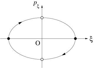
For any small nonzero , one may find a value of for which is so large that the two above-mentioned stationary points can be treated separately in the SPM. At the same time, can be sufficiently small that the stationary points are much smaller than the integration limits . In practice, it is enough to consider and , and we split the integration interval into two parts, i.e., from to and from to , in order to separate the contributions of negative and positive stationary points and . According to the phase-space flow around the PO (see Fig. 1), the curvature ( denotes the momentum conjugate to ) will always change its sign from positive to negative at the caustic catastrophe point Ozoriobook .
Let us consider such crossings with a catastrophe point. Outside the catastrophe point, where , the stationary point corresponds to and its contribution is given by the second integral over positive . For this integral, one can extend the upper integration limit to infinity, like in the SSPM, because and for a small finite [see Eq. (19)]. Within this approximation, one can use the standard complete Airy and Gairy functions
| (22) |
They correspond to the limits and in Eq. (18). Using the asymptotic form of the Airy and Gairy functions for ,
| (23) |
one can evaluate the contribution of the positive stationary point to Eq. (III.1), asymptotically far from the caustic point (III.1). Then one obtains the same result as one would get by the standard second-order expansion of the phase (and zeroth order of the amplitude ) at a simple stationary point ,
| (24) |
On the other side of the crossing with the catastrophe point, , the stationary point corresponds to . Therefore, one should consider the other part of the integral over the negative values of . Obviously, considering in an analogous way with a change of the integration variable , one obtains
| (25) |
Comparing the rightmost expression in Eq. (25) with that in Eq. (24), one sees a shift of phase by . Thus, the famous Maslov theorem MASLOV on the shift of the phase by at each simple caustic point (III.1) of the CT (in particular, the PO) in the SSPM (i.e., the Maslov index is increased by one) has been proved by using the Fedoriuk catastrophe method FEDoryuk_pr .
For the case of a turning point, one has the conditions (III.1) with only the replacement of zero by infinity in the second derivative. In this case, Fedoriuk used a linear coordinate transformation from to , which has the form
| (26) |
where and are new constants that are not singular in ( is independent of ). This transformation reduces the turning-point singularity to the caustic-point one. Indeed, the divergent second derivative of the phase over the variable is transformed, in a new variable, to its zero value
| (27) |
(see the second paper in Ref. FEDoryuk_pr ). Therefore, one obtains the same shift by at each simplest turning point (per a sign change of one momentum component perpendicular to the boundary) along a CT. Finally, the next part of the Maslov theorem MASLOV concerning the Maslov index generated by such a turning point has been proved, too, within the same catastrophe theory of Fedoriuk FEDoryuk_pr .
IV Symmetry-breaking and bifurcations
Assuming a convergence of the expansion [Eq. (10)] to the second order, as shown in the preceding section, one can use the same approach within the simplest ISPM2 of second order222We call the th-order ISPM the ISPM, in which we use the expansion of the phase integral up to the th-order terms and the amplitude up to the th order near the stationary point. The simplest ISPM for is called the ISPM2. to investigate the symmetry-breaking and bifurcation problems in the POT. Therefore, one arrives at a sum over the separate contributions of different kinds of isolated and degenerated orbits, as in the derivation of the Maslov theorem but within the finite integration limits. The latter is important because the bifurcation point is located at a boundary of the classically accessible region. This section is devoted to the extension of the FMCT to the bifurcation catastrophe problems.
In the presence of continuous symmetries, the stationary points form a family of POs that cover a -dimensional submanifold of phase space, whereby is the classical degeneracy of the PO family. The integration over must be performed exactly. In any systems with continuous symmetries, it is an advantage to transform the phase-space variables from the Cartesian to the corresponding action-angle variables (see, e.g., Ref. BT76 ; CREAGHpra97 ). Then the action in Eq. (II) is independent of the angle variables conjugate to the conserving action variables and the integrations over these cyclic angle variables are exactly carried out. For the integrable case, for instance, integrating over the remaining action variables and using the standard SPM, one obtains the so-called Berry-Tabor trace formula BT76 . Under the existence of additional symmetries such as SU(3) or O(4), some of the integrations over the action variables can also be performed exactly because of a higher degeneracy. For partially integrable systems, the integrations over partial set of cyclic variables also greatly simplify the ISPM derivations of the trace formula (II) near the bifurcations.
To solve the bifurcation problems, some of the SPM integrations have to be done in a more exact way. For definiteness, we will consider first a simple bifurcation defined as a caustic point of the first order [Eqs. (10) and (11)] where the degeneracy parameter is locally increased by one. In the SPM, after performing exact integrations over a submanifold , one uses an expansion of the action phase in phase space variables , perpendicular to in the integrand of Eq. (II) over near the stationary point ,
| (28) |
where
| (29) |
is the stationary point, , and . To demonstrate the key point of our derivations of the trace formula, we focus on one of the phase-space variables in Eq. (II), denoted by , which is associated with a catastrophe behavior. In the standard SPM, the above expansion is truncated at the second-order term and the integration over the variable is extended to . The integration can be performed analytically and yields a Fresnel integral (see, e.g., Refs. sclbook ; migdalrev ).
However, one encounters a singularity in the SSPM that is related to the zero or infinite value of , while remains finite in the simplest case under consideration. This singularity occurs when a PO (isolated or degenerated) undergoes a simple bifurcation at the stationary point under the variation of a parameter of the potential (e.g., energy, deformation, or surface diffuseness). The SSPM approximation to the Fresnel (error) functions by the Gaussian integrals breaks down because one has a divergence.
Notice that the bifurcation problem is similar to the caustic singularity considered by Fedoriuk within the catastrophe theory (see Sec. III and Refs. FEDoryuk_pr ; FEDoryuk_book1 ). The FMCT is adopted, however, for the specific position of such a singularity at the end point in the phase-space volume accessible for a classical motion (see the Introduction and also Ref. MAFptp06 ).
In systems with continuous symmetries, the orbit at the end point causes the bifurcation where it coincides with one of the rational tori that appears in the transition from the unphysical to the physical region. The contribution of this end-point orbit is derived using a local phase-space variable along it, independently of the torus orbits. Near the bifurcation point, the contribution of these end-point orbits is mostly included to the newborn orbit term. Therefore, we should consider a kind of separation of the phase space occupied by the newborn and end-point orbits to evaluate their contributions to the trace integral near the bifurcation point. Below we will call the latter an end-point manifold. By definition of the end-point manifold, its measure is zero at the bifurcation limit where the minimal and maximal coincide with the stationary point , i.e.,
| (30) |
Thus, although the contributions of POs participating in the bifurcation are considered separately, the parent orbit contribution vanishes at the bifurcation point and there no risk of double counting. To describe the transition from the bifurcation point to the asymptotic region, one should properly define the end-point manifold. We need it to extract the additional contribution by the end-point orbit that is not covered by the term for the newborn orbit. The detailed treatment of such a transition is still open, but is beyond the scope of the present paper.
We are ready now to employ what we call the improved stationary-phase method MFAMMSBptp99 ; MFAMBpre01 ; MAFMptp02 ; MAFptp06 evaluating the trace integral for the semiclassical level density. Hereby, the integration over in Eq. (II) is restricted to the finite limits defined by the classically allowed phase-space region through the energy-conserving function in the integrand of Eq. (II). The phase and amplitude are expanded around the stationary point up to the second- and zeroth-order terms in , respectively, and to higher-order terms if necessary.
In the simplest version of the ISPM (ISPM2), the expansion of the phase is truncated at second order, keeping the finite integration limits and given by the accessible region of the classical motion in Eq. (II). It will lead to a factor like333 For the case of several variables for which we find find zeros and infinities in eigenvalues of the matrix with second-order derivatives of at , we diagonalize this matrix and reduce the Fresnel-like integrals to products of error functions similar to Eq. (IV).
| (31) |
where is the generalized error function,
| (32) |
with the complex arguments
| (33) |
Note that the expression (IV) has no divergence at the bifurcation point where , since the error function (32) also goes to zero as
| (34) |
Thus, the factor in the denominator of Eq. (IV) is canceled with the same in the numerator. In addition, also taking into account Eq. (30) and the discussion around it, one finds the zero contribution of the end-point term in the trace formula at the bifurcation point, which seems to be a consistent semiclassical picture.
This procedure is proved to be valid in the semiclassical limit by the FMCT FEDoryuk_pr ; MASLOV ; FEDoryuk_book1 . In this way, we can derive the separate PO contributions that are free of divergences, discontinuities, and double counting at any bifurcation point. The oscillating part of the level density can be approximated by the semiclassical trace formula (6). In Eq. (6), the sum runs over all periodic orbits (isolated or degenerated) in the classical system. The term is the action integral along a PO. The amplitude (which, in general, is complex) is of the order of the phase-space volume occupied by CTs. The factor given in Eq. (IV) depends on the degeneracies and stabilities of the POs, respectively (see Sec. III).
Notice that any additional exact integration in Eq. (II) with respect to a bifurcation (catastrophe) variable of the improved SPM can lead to an enhancement of the amplitude in the transition from the bifurcation point to the asymptotic region. This enhancement is of the order as compared to the result of the standard SPM integration. In particular, for the newborn family with the extra degeneracy higher than that of the parent PO, one has such enhancements of the order near the bifurcation.
The trace formula (6) thus relates the quantum oscillations in the level density to quantities that are purely determined by the classical system. Therefore, one can understand the shell effects in terms of classical pictures. The sum over POs in Eq. (6) is asymptotically correct to the leading order in and it is hampered by convergence problems GUTZbook90 . However, one is free from those problems by taking the coarse-grained level density
| (35) |
where is an averaging width. The value of is sufficiently smaller than the distance between the major shells near the Fermi surface (see Refs. BBann72 ; SMepp76 ; SMODzp77 ; sclbook ; migdalrev ; MKApan16 ). Here is the period of the particle motion along a PO taking into account its repetition number. We see that, depending on the smoothing width , longer orbits are automatically suppressed in the above expressions and the PO sum converges, which it usually does not GUTZbook90 for nonintegrable systems in the limit . Thus, one can highlight the major-shell structure in the level density using a smoothing width that is much larger than the mean single-particle level spacing but smaller than the main shell spacing (the distance between major shells) near the Fermi surface. Alternatively, a finer shell structure can be considered by using essentially smaller smoothing widths, which is important for studying the symmetry-breaking (bifurcation) phenomenon associated with longer POs.
It is an advantage of this approach that the major-shell effects in can often be explained semiclassically in terms of only a few of the shortest POs in the system. Examples will be given in Sec. V. However, if one wants to study a finer shell structure, specifically at large deformations, some longer orbits have to be included. Hereby, bifurcations of POs play a crucial role, as it will be exemplified in Sec. V.
V ISPM for the spherical RPL potential model
Let us apply the general FMCT to the RPL potential as an analytically solvable example.
V.1 Scaling property
A realistic mean-field potential for nuclei and metallic clusters is given by the well-known Woods-Saxon (WS) potential
| (36) |
where is the depth of the potential, is the nuclear radius, and is the surface diffuseness. As suggested in Refs. KAijmpe04 ; KAprc12 , this potential can be approximated by the RPL potential for a wide range of mass numbers as
| (37) |
with an appropriate choice of the radial power parameter . One finds good agreement of the quantum spectra for the approximation (37) to the WS potential up to and around the Fermi energy . Eliminating the constant term on the right-hand side of (37), we define the RPL model Hamiltonian as
| (38) |
where is the mass of a particle and is an arbitrary length parameter.
In the spherical RPL model (38), as well as in general spherical potential models, one has the diameter and circle POs that form the two-parameter () families. The diameter and circle POs have minimum and maximum values of the angular momentum and , respectively. They correspond to the end points of the energy surface implicitly given by the relationship (see, e.g., Ref. MKApan16 )
| (39) |
where is the radial momentum
| (40) |
with the particle momentum
| (41) |
The integration limits and in Eq. (39) are functions of the energy and angular momentum for a given spherical potential . In the spherical RPL potential, they are defined by the two real roots of the transcendent equation for the variable :
| (42) |
Another key quantity in the POT is the curvature of the energy surface (39)
| (43) |
Using the invariance of the equations of motion under the scale transformation
| (44) |
one may factorize the action integral along the PO as
| (45) |
In Eq. (V.1) we define the dimensionless variables and as classical characteristics of the particle motion
| (46) |
and
| (47) |
We call them the scaled energy and the scaled period, respectively. To realize the advantage of the scaling invariance under the transformation (V.1), it is helpful to use and in place of the energy and the period for the particle motion along a PO, respectively. In the harmonic-oscillator (HO) limit (), and are proportional to and , while in the cavity limit (), they are proportional to the momentum and the geometrical PO length , respectively.
The PO condition (II) determines several PO families in the RPL potential, namely, the polygonlike (), the circular, and the diametric () POs. This condition for the integrable spherical Hamiltonian is identical to a resonance condition, which is expressed in the spherical variables as
| (48) |
where , , and are frequencies in the radial and angular motion. Figure 2 shows these POs in the RPL potential (38) in the plane, where is the scaled period for the PO specified by , which satisfies the resonance condition (48).
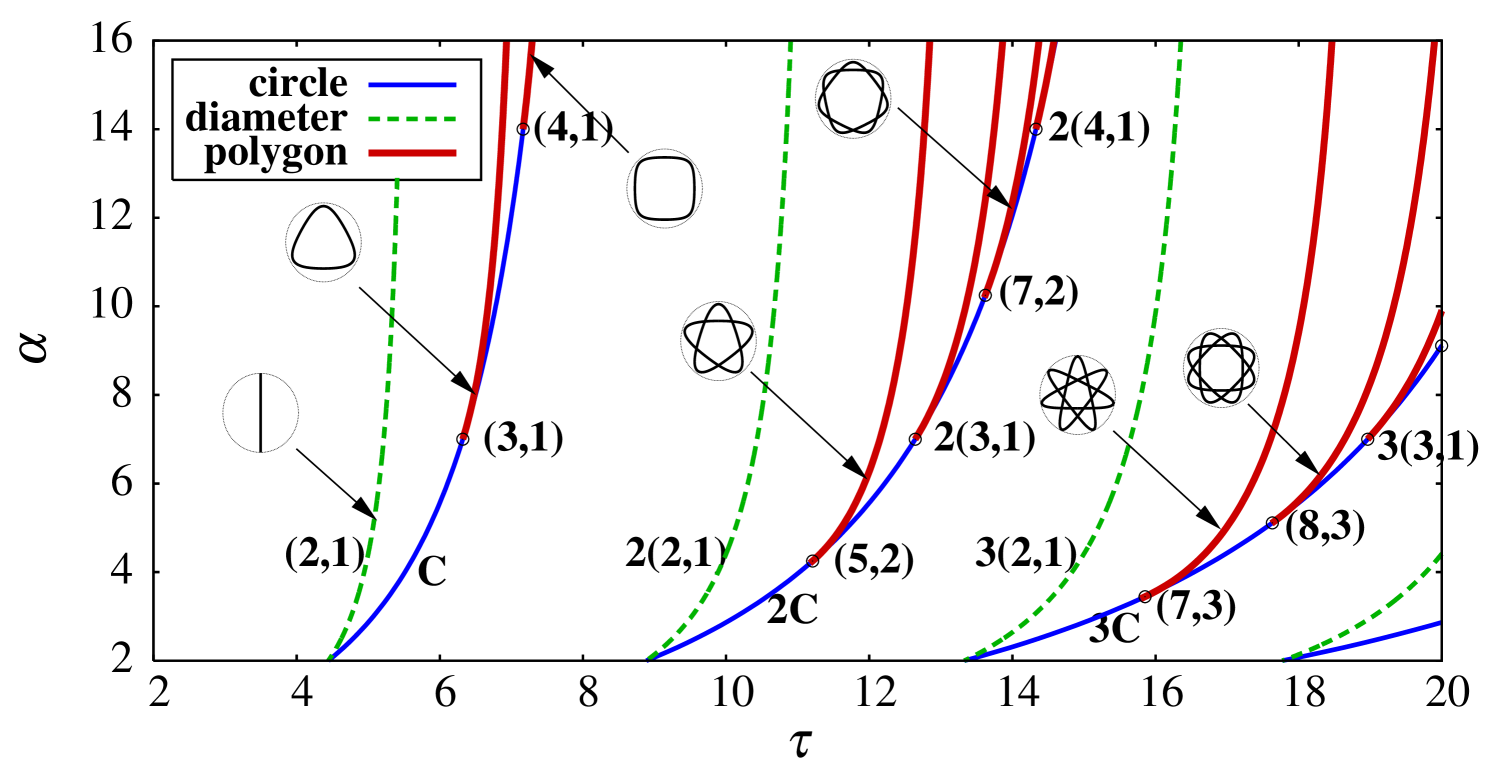
As shown in this figure, the polygonlike orbit continues to exist after its emergence at the bifurcation point from the parent circular orbit (th repetition of the primitive circle orbit ). The exceptions are the diameter orbits (2,1) that exist for all values of and form families with a higher degeneracy at the HO symmetry-breaking point .
V.2 Three-parameter PO families
For the contribution of the three-parameter () families into the density shell correction [Eq. (II)], one obtains MKApan16
| (49) | |||||
The sum is taken over families of the three-parameter () polygonlike orbits ( stands for polygonlike, and for the repetition number ). In Eq. (49), is the action along the PO,
| (50) |
where is the radial action variable in the spherical phase-space coordinates [Eq. (39)]. The angular momentum is given by the classical value for a particle motion along the orbit in an azimuthal plane. The numbers and specify the orbit with . For the amplitude [Eq. (49)], within the ISPM2, one finds
| (51) |
where represents the curvature (43) at and is the period of the primitive () polygonlike orbit, . For a three-parameter family at the stationary point determined by the PO (stationary-phase) equation, one has
| (52) |
The function in Eq. (51) is given by the generalized error function (32). Its complex arguments are expressed in terms of the curvature ,
| (53) |
We used here the ISPM2 for the finite integration limits within the tori, i.e., between the minimal and maximal values of the angular-momentum integration variable for the family contribution. The phase factor in Eq. (49) is the Maslov index (see Sec. III) as in the asymptotic Berry-Tabor trace formula. The amplitude (51) obtained for the formula (49) is regular at the bifurcation points where the stationary point is located at the end point of the action () part of a torus.
For the case of the power parameter sufficiently far from the bifurcation points, one arrives at the SSPM limit of the trace formula (49) with the amplitude , identical to the Berry-Tabor trace formula BT76
| (54) |
According to Sec. III, the Maslov index of Eq. (49) is determined by the number of turning and caustic points within the FMCT (see Refs. FEDoryuk_pr ; MASLOV ; FEDoryuk_book1 ; MAFptp06 ),
| (55) |
The total Maslov index is defined as the sum of this asymptotic part (55) and the argument of the complex density amplitude (51) migdalrev ; MAFMptp02 ; MAFptp06 ; MFAMMSBptp99 ; MKApan16 . The total index behaves as a smooth function of the energy and the power parameter through the bifurcation point.
V.3 Two-parameter circle families in the ISPM2
For contributions of the circular PO families to the trace formula (II), one obtains
| (56) | |||||
The sum is taken over the repetition number for the circle PO and . Here is the action along the orbit ,
| (57) |
where is the angular momentum of the particle moving along the orbit . For amplitudes of the -orbit contributions, one obtains
| (58) | |||||
where is the period of a particle motion along the primitive () orbit C. Here, is the azimuthal frequency,
| (59) |
the radius of the orbit, and is the angular momentum for a particle motion along the PO KAprc12 ; KAijmpe04 ; MVApre13 ; MKApan16 ,
| (60) |
In Eq. (58), is the stability factor (the trace of the monodromy matrix)
| (61) |
and is the Jacobian
| (62) |
where is the curvature for orbits MVApre13 ,
| (63) |
The finite limits in the error functions of Eq. (58), and , are given by
| (64) |
where and are the radial turning points specified below. The interval between them covers the CT manifold including the stationary point .
Asymptotically far from the bifurcations (also far from the symmetry breaking point ), the amplitude (58) approaches the SSPM limit
| (65) |
In these SSPM derivations, the radial integration limits and turn into the asymptotic values
| (66) |
They are given by the two real solutions of Eq. (42) at . The upper limit was extended to infinity in the derivation of Eq. (65) because the stationary point is far away from both integration boundaries and .
The Maslov index in Eq. (56) is given by
| (67) |
For the calculation of this asymptotic Maslov index through the turning and caustic points [see the trace formula (56) with the ISPM2 (58) and the SSPM (65) amplitude], one can use the FMCT (Sec. III). The total Maslov index can be introduced as above (see Refs. migdalrev ; MAFMptp02 ; MAFptp06 ; MFAMMSBptp99 ; MKApan16 ).
Taking the opposite limit to the bifurcations where , but far away from the HO limit , one finds that the argument of the second error function in Eq. (58), coming from the radial-coordinate integration, tends to zero proportional to [Eq. (V.3)]. Thus, as in a general case (Sec. IV), the singular stability factor of the denominator in Eq. (58) is exactly canceled by the same from the numerator. At the bifurcation , one obtains
| (68) | |||||
Therefore, Eq. (58) gives the finite result through the bifurcation. Taking the reduction of the end-point manifold for the parent-orbit term, according to Eq. (30),
| (69) |
the amplitude (58) vanishes at the bifurcation point MKApan16 [see Eq. (68)]. This is in line with general arguments for the bifurcation limit [see Sec. IV around Eq. (30)].
As shown in the Appendix, following the FMCT (Sec. III) one can derive the ISPM3 expression for the oscillating level density. One may note that the parameter given by Eq. (87) can be considered as the dimensionless semiclassical measure of the distance from a bifurcation. Similarly, as for the caustic catastrophe points, in the case of the application of the FMCT (Sec. III) to the bifurcation of the circular orbits (see also Sec. V), one can use simply the ISPM2 (Sec. V.3) as the simplest approximation near the bifurcation, i.e., . However, working out properly the transition itself from the asymptotic SSPM radial-integration limits to the same value at the bifurcation within its close vicinity () is left for future work.
V.4 Two-parameter diameter families
For the diameter-orbit () family contribution to the trace formula (II) for the RPL potential, the ISPM is needed only near the symmetry-breaking at of the harmonic-oscillator limit MKApan16 . For our purpose, we simply use the SSPM approximation for the diameter families, valid at the values of the power parameter far from the symmetry-breaking limit,
| (70) |
where
| (71) |
The frequency is expressed through the radial period,
| (72) |
where is the Gamma function. In Eq. (71), is the diameter curvature MVApre13
| (73) |
For the Maslov index [Eq. (V.4)], one obtains
| (74) |
V.5 TOTAL TRACE FORMULAS FOR THE SPHERICAL RPL POTENTIAL
The total ISPM trace formula for the RPL potential is the sum of the contribution of the polygonlike () families [Eqs. (49) with (51)], the circular () families [Eqs. (56) and (58) for the ISPM2 and Eqs. (A) and (A) for the ISPM3], and the diameter () families [Eqs. (V.4) and (71)],
| (75) |
This trace formula has the correct finite asymptotic limits to the SSPM: The Berry-Tabor result [Eqs. (49) and (54)] for the orbits () and for orbits () [Eqs. (56) and (65)]; see the same for orbits [Eqs. (V.4) and (71)]. Transforming the variable from the ordinary energy to the scaled energy (46), one obtains the trace formula for the scaled-energy level density,
| (76) |
with
| (77) |
The Fourier transform of this scaled-energy level density, truncated by the Gaussian with the cutoff , is expressed as
| (78) |
This gives a function with successive peaks at the scaled periods of the classical POs with the height , which is proportional to the amplitude of the contribution of the orbit PO to the semiclassical level density. Evaluating the same Fourier transform by the exact quantum level density, one has
| (79) | |||||
with
| (80) |
Thus, one can extract the contribution of classical periodic orbits to the level density from the Fourier transform of the quantum level density. In what follows we consider the classical-quantum correspondence using this Fourier transformation technique, in addition to the direct comparison of quantum and semiclassical level densities.
VI Comparison with quantum results

Figure 3 shows the Fourier transform of the quantum-mechanical level density for the RPL potential [see Eq. (79)]. At the HO limit , all the classical orbits are periodic and form the four-parameter family for a given energy. The Fourier transform exhibits the equidistant identical peaks at , corresponding to the th repetitions of the primitive PO family. With increasing , each peak is split into two peaks corresponding to the diameter () and circle () orbits and the amplitudes of the oscillating level density for these orbits are decreased. However, one finds a growth of the peak at corresponding to the orbit around the bifurcation point . Note that, approaching the bifurcation, the contribution of the orbit is strongly enhanced until it forms a local family of POs with a higher degeneracy at the bifurcation point. From this point a trianglelike (3,1) family bifurcates. This family has high degeneracy . It remains important, also for larger . The above enhancement in the Fourier peaks is directly associated with the oscillating ISPM level-density amplitude of the bifurcating PO family having a high degeneracy. This family is a major term in the expansion in the comparison with the SSPM asymptotics (see Sec. IV and Ref. MKApan16 ). The Fourier peak at in Fig. 3 shows the enhancement of the amplitude of the newborn (3,1) family contribution including (1,1) orbits as the end points (see the Introduction and Sec. IV).
As the significance of bifurcations is confirmed through the Fourier analysis [Eqs. (78) and (79)], let us now investigate the oscillating part of the scaled-energy level densities averaged with the Gaussian averaging parameter ,
| (81) |
The semiclassical shell-correction density is given by
| (82) |
[see Eq. (77) for ]. For the quantum density, one has
| (83) |
where
| (84) |
The smooth level density is calculated for the scaled spectrum . For these calculations we employed the standard Strutinsky averaging (over the scaled energy ), finding a good plateau444 It may worth pointing out that the quality of the plateau in the SCM calculations of the level density is much better when using the scaled-energy variable rather than the energy itself MVApre13 . around the Gaussian averaging width and curvature-correction degree .
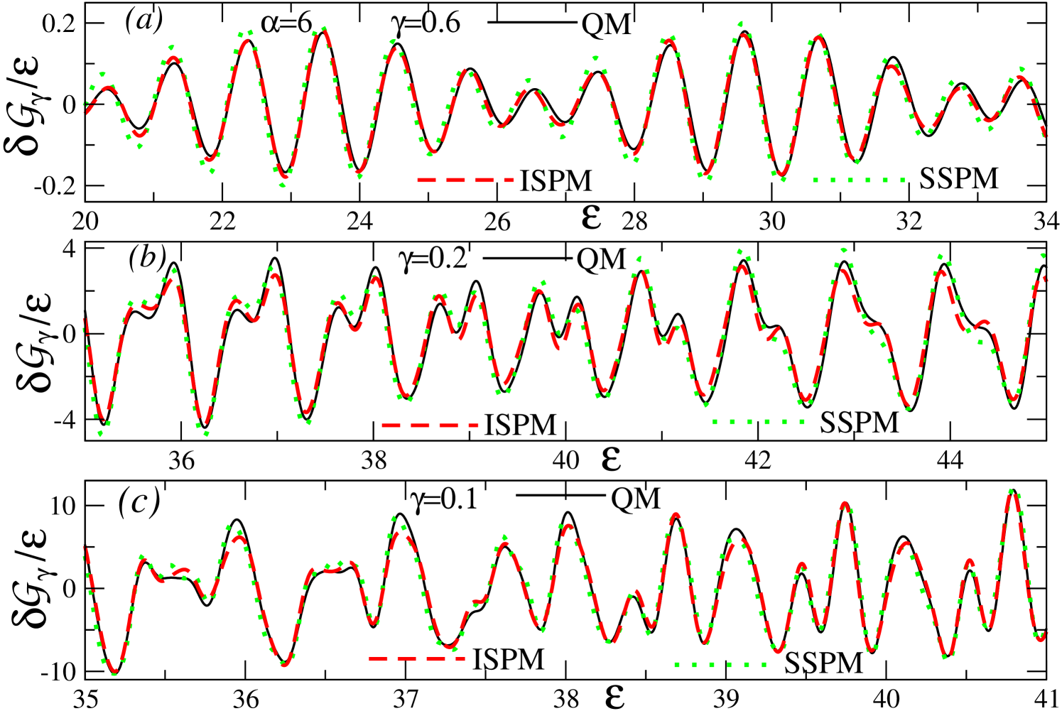
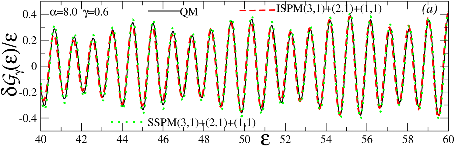
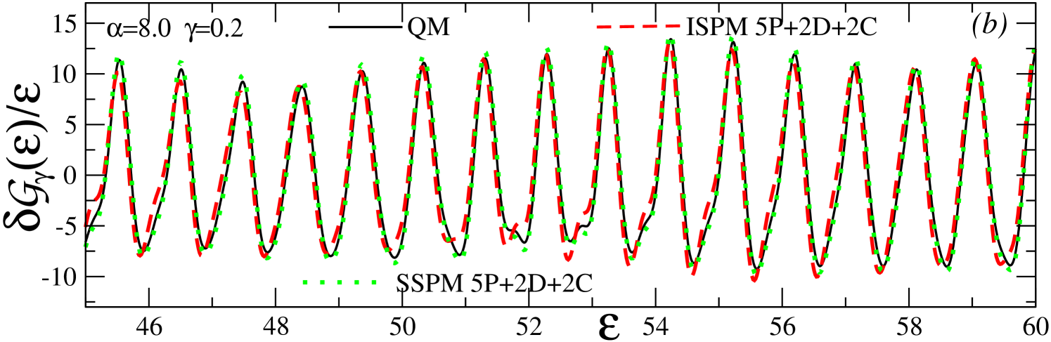
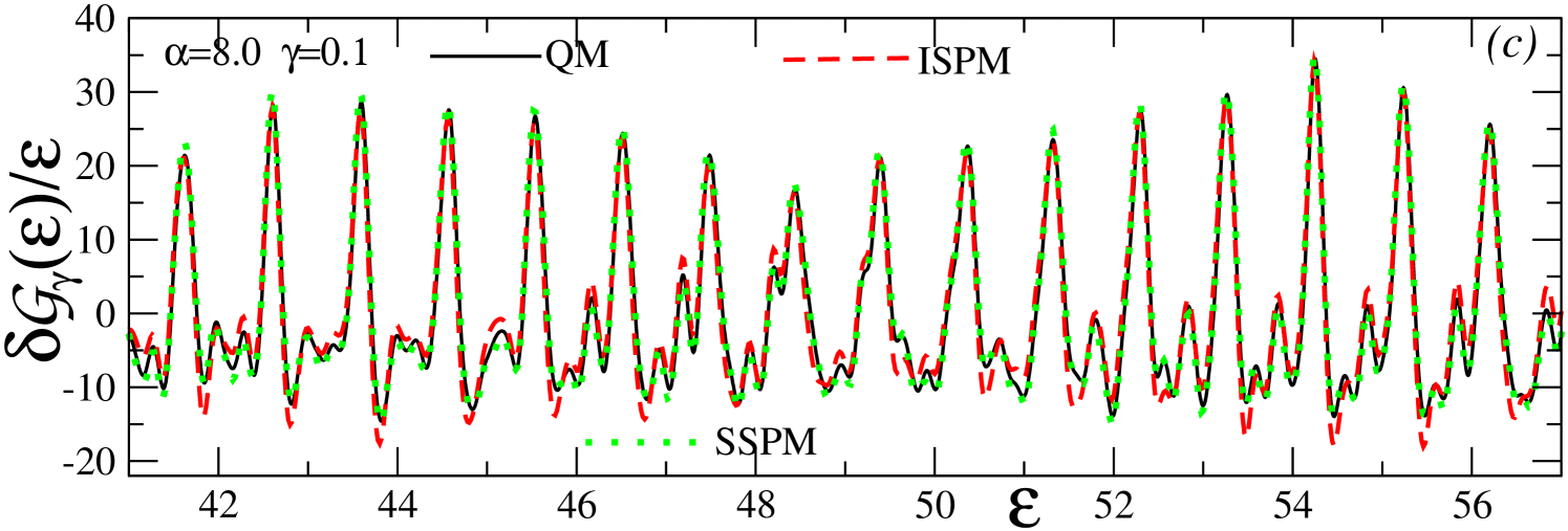
Figures 4–6 show good agreement of the coarse-grained () and fine-resolved () semiclassical and quantum results for (divided by ) as functions of the scaled energy at , and . At , as well as and , the analytic expressions for all of the classical PO characteristics are available, and can be used to check the precision of the numerical calculations MVApre13 ; MKApan16 . The values (Fig. 4) and (Fig. 6) are taken as examples that are sufficiently far from the bifurcation point (Fig. 5). The ISPM results at these values of show good convergence to the SSPM results. The and POs with the shortest (scaled) periods are dominating the PO sum at a large averaging parameter (the coarse-grained or major-shell structure). Many more families with a relatively long period at (the fine-resolved shell structure) become significant in comparison with the quantum results MKApan16 .
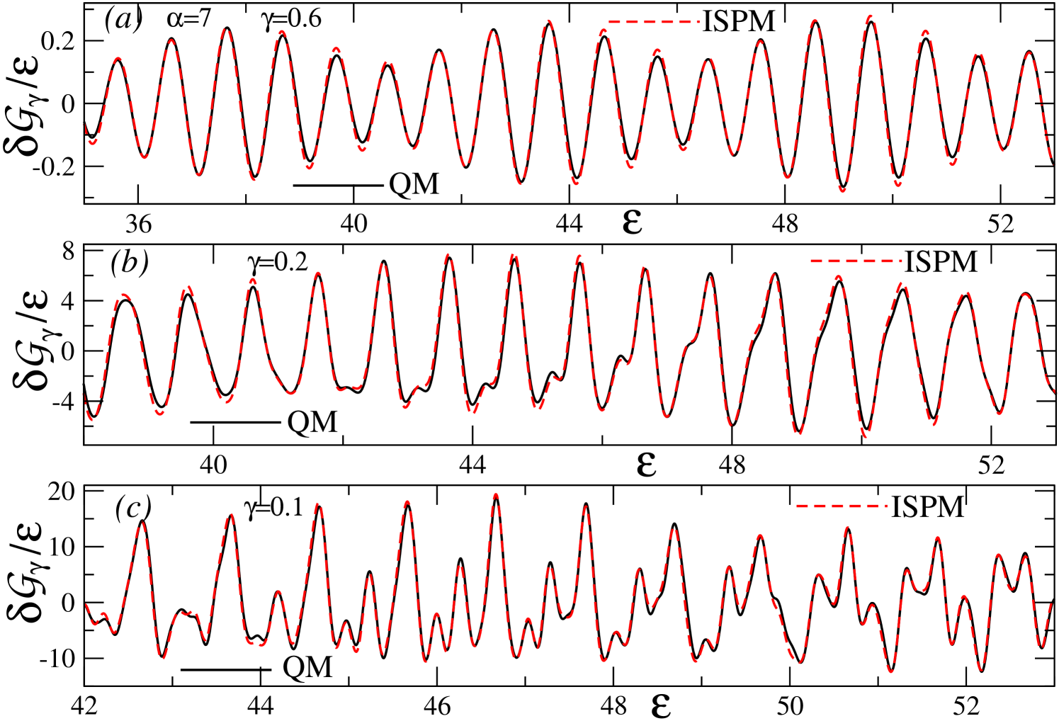
Figure 5 shows the results for the bifurcation point where the trianglelike (3,1) PO family emerges from the parent (1,1) family in a typical bifurcation scenario. One also finds good agreement of the ISPM with quantum results here. As the SSPM approximation fails at the bifurcation, it is not presented in Fig. 5. As discussed above, the SSPM at the bifurcation yields a sharp discontinuity of the (3,1) amplitude and a divergent behavior of the (1,1), in contrast to the continuous ISPM components. Our results in Fig. 5 demonstrate that the ISPM successfully solves these catastrophe problems of the SSPM for all averaging parameters . In contrast to the results shown in Figs. 4 and 6, the coarse-grained () density oscillations at the bifurcation point (Fig. 5) do not contain any contributions from the (1,1) end-point term but instead the (3,1) term becomes dominant.
Note that many more families with relatively long periods become necessary to account for the fine-resolved shell structures () MKApan16 . For the exemplary bifurcation , at smaller averaging parameters () the dominating orbits become the bifurcating newborn (3,1) of the highest degeneracy along with the leading (5,2), (7,3), and (8,3) POs which are born at smaller (see Fig. 2). They include the parent -orbit end-point manifolds. As also shown in the quantum Fourier transforms in Fig. 3, these POs yield larger contributions at the bifurcation values of and are even more enhanced on their right in a wide region of .
VII Conclusions
The Fedoriuk-Maslov catastrophe theory is extended to simple bifurcation problems in the POT. Within the extended FMCT, we overcome the divergence and discontinuity of semiclassical amplitudes of the standard stationary-phase method, in particular, in the Berry-Tabor formula near bifurcations. A fast convergence in the PO expansion of the averaged level density for a large Gaussian averaging parameter is shown too. This allows one often to express significant features of the shell structure in terms of a few short periodic orbits. We have formulated our ISPM trace formula for a simple bifurcation scenario so that the parent orbits at the end points have vanishing contributions at the bifurcation point, which allows us to consider them everywhere separately from the term for a newborn family of the periodic orbits.
The extended FMCT is used for derivations of the trace formula in the case of the three-dimensional spherical RPL potential by employing the improved stationary phase method. We presented a class of the radial power-law potentials that, up to a constant, provides a good approximation to the WS potential in the spatial region where the particles are bound. The RPL potential is capable of controlling surface diffuseness and contains the popular harmonic-oscillator and cavity potentials in the two limiting cases of the power parameter . Its advantage is the scaling invariance of the classical equations of motion. This invariance makes the POT calculations and the Fourier analysis of the level density very easy. The contribution of the POs to the semiclassical level density and shell energies is expressed analytically (and even all the PO characteristics are given explicitly, e.g., for ) in terms of the simple special functions. The quantum Fourier spectra yield directly the amplitudes of the quantum level density at the periods (actions) of the corresponding classical POs.
We have derived the semiclassical trace formulas that are also valid in the bifurcation region and examined them at the bifurcation catastrophe points and asymptotically far from them in the spherical RPL potential model. They are based on the SPM improved to account for the effect of the bifurcations by using the extended FMCT. The ISPM overcomes the problems of singularities in the SSPM and provides the generic trace formula that relates the oscillating component of the level density for a quantum system to a sum over POs of the corresponding classical system. We showed good convergence of this improved trace formula to the simplest ISPM based on the second-order expansion of the classical action at several characteristic values of the power parameter including the bifurcations and asymptotically far from them.
We obtained good agreement between the ISPM semiclassical and quantum results for the level-density shell corrections at different values of the power parameter , both at the bifurcations and far from them. Sufficiently far from the bifurcation of the leading short POs with a maximal degeneracy, one finds also good convergence of the ISPM trace formulas to the SSPM approximation. We emphasize the significant influence of the bifurcations of short POs on the main characteristics of oscillating components of the single-particle level density for a fermionic quantum system. They appear in the significant fluctuations of the energy spectrum (visualized by its Fourier transform), namely, the shell structure.
In line with the general arguments of the extended FMCT, the stationary points forming the circular-orbit families are located at the end point of the classically accessible region and they coincide with the newborn family of the polygonlike orbits at the bifurcation. Taking into account the reduction of the end-point manifold in the bifurcation limit, the parent -family contribution is transformed into the newborn -family term that presents now their common result. Thus, one has the separate contributions of the parent and newborn orbits through the bifurcation scenario, but with no concern about double counting.
Future work should study in detail the transition of the ISPM trace formula from the bifurcation points to its asymptotic SSPM region. This will enable us to understand more properly the shape dynamics of the finite fermion systems. In particular, the improved stationary phase method can be applied to describe the deformed shell structures where bifurcations play an essential role in formations of the superdeformed minima along a potential energy valley migdalrev ; MKApan16 . One of the remarkable tasks might be to clarify, in terms of the symmetry-breaking (restoration) and bifurcation phenomena, the reasons of the exotic deformations such as the octupole and tetrahedral ones within the suggested ISPM. In this way, it would be worth extending our present local bifurcation FMCT to describe, e.g., a bridge (non-local) bifurcation phenomenon found in a more realistic mean field in the fermionic systems (see also Refs. KAprc12 ; AMprc14 ; KAps16 ; KAps17 ).
Our semiclassical analysis may therefore lead to a deeper understanding of the shell effects in the finite fermionic systems such as atomic nuclei, metallic clusters, trapped fermionic atoms, and semiconductor quantum dots sclbook ; ABjpa08 ; RBMpra96 ; BBCzp97 ; FKMSprb08 ; BO05 . Their level densities, conductance, and magnetic susceptibilities are significantly modified by shell effects. As a first step towards the collective dynamics, the oscillating parts of the nuclear moment of inertia should be studied semiclassically in terms of POs taking into account the bifurcations MSKBprc10 ; MGBpan14 ; GMBBprc16 ; MGBpan17 .
ACKNOWLEDGMENTS
The authors gratefully acknowledge M. Brack and K. Matsuyanagi for fruitful collaborations and many useful discussions. One of us (A.G.M.) is also very grateful for hospitality during his working visits to the Department of Physical Science and Engineering of the Nagoya Institute of Technology and for financial support from the Japanese Society of Promotion of Sciences through Grant No. S-14130.
Appendix A The ISPM3 approximation
Following the FMCT (Sec. III), one can derive the improved (ISPM3) contribution of the orbits by taking into account the third-order terms of the action expansion [see Eq. (10)] in the integration over the catastrophe variable . Within the ISPM3, one obtains
| (85) |
The ISPM3 amplitudes are given by
| (86) |
where
| (87) |
with
| (88) |
The parameter of Eq. (8) [Eq. (12)] used in deriving the above expressions is proportional to the stability factor [Eq. (61)],
| (89) |
The incomplete Ai (Gi) integrals in Eq. (A) are defined by Eq. (18). The integration limits of these functions are the same as those given by Eq. (20),
| (90) |
where are the upper () and lower () limits for the radial integration. These integration limits are defined in Eq. (66). In the bifurcation limit , both terms in square brackets in Eq. (A) [see also Eq. (90)] go to zero for the same reason as in the ISPM2 case. The incomplete Ai and Gi functions of the integrand [Eq. (18)] have no singularities in the bifurcation limit . In addition, the radial integration limits and approach the stationary point , which is the -orbit radius [Eq. (69)]. This ensures the disappearance of the end-point manifold in this limit and therefore, in line with the general arguments of Sec. IV (see also Sec. V.3), one finds the zero contribution of the circular orbit term exactly at this bifurcation. In turn, the contribution of the circular orbit is included in the newborn orbit term.
In the opposite limit, sufficiently far from the bifurcation points, where the stability factor takes a finite nonzero value, the second term in Eq. (90) changes with increasing much faster (proportional to ) than the first component (proportional to ). Thus, one has in this limit. The ISPM3 expression [Eq. (A) with Eq. (A)] for the oscillating level density suggests that the parameter () can be considered as a dimensionless measure of the distance from the bifurcation [see Eqs. (87) and (89)]. For a large distance from the bifurcation [Eq. (87)], one can extend the radial integration limits as and . In this limit, the incomplete Airy and Gairy functions (18) can be approximated by the complete ones (22). Since the argument of these standard functions [Eq. (87)] at a finite stability factor becomes large in the semiclassical limit , one can use their asymptotic expressions (23). Thus, we arrive at the same SSPM result [Eqs. (56) and (65)] for the family contributions as obtained from the ISPM2 -trace formula [see Eq. (A) for its amplitude].
For the simplest catastrophe problem, the ISPM3 might become important when the PO is distant from the bifurcation points to some extent but not asymptotically far from them. It is also necessary for the higher-order catastrophe problem, which is not found in the RPL model discussed in this paper. The definition of the end-point manifold might also be affected by the consideration of higher expansion terms. This is also a problem to be solved in the future in order to describe the transition from a bifurcation vicinity to the asymptotic region.
References
- (1) M. C. Gutzwiller, J. Math. Phys. 12, 343 (1971).
- (2) M. C. Gutzwiller, Chaos in Classical and Quantum Mechanics (Springer, New York, 1990).
- (3) R. B. Balian and C. Bloch, Ann. Phys. (N.Y.) 69, 76 (1972).
- (4) M. Brack and R. K. Bhaduri, Semiclassical Physics (Westview, Boulder, 2003).
- (5) V. M. Strutinsky, Nucleonica, 20, 679 (1975); V. M. Strutinsky and A. G. Magner, Sov. J. Part. Nucl., 7, 138 (1976) [Fiz. Elem. Chastits At. Yadra, 7, 356 (1976)].
- (6) V. M. Strutinsky, A. G. Magner, S. R. Ofengenden, and T. Døssing, Z. Phys. A 283, 269 (1977).
- (7) A. G. Magner, Sov. J. Nucl. 28, 759 (1978) [Yad. Fiz. 28, 1477 (1978)].
- (8) S. C. Creagh, J. M. Robbins, and R. G. Littlejohn, Phys. Rev. A 42, 1907 (1990); S. C. Creagh, R. G. Littlejohn, ibid. 44, 836 (1991); J. Phys. A 25, 1643 (1992).
- (9) M. V. Berry and M. Tabor, Proc. R. Soc. London Ser. A 349, 101 (1976); 356, 375 (1977).
- (10) A. G. Magner, I. S. Yasyshyn, K. Arita, and M. Brack, Phys. Atom. Nucl. 74, 1445 (2011) [Yad. Fiz. 74, 1475 (2011)].
- (11) A. G. Magner, M. V. Koliesnik, and K. Arita, Phys. Atom. Nucl. , 79, 1067 (2016).
- (12) A. G. Magner, K. Arita, S. N. Fedotkin, and K. Matsuyanagi, Prog. Theor. Phys. 108, 853 (2002).
- (13) A. G. Magner, K. Arita, and S. N. Fedotkin, Prog. Theor. Phys. 115, 523 (2006).
- (14) A. G. Magner, S. N. Fedotkin, K. Arita, T. Misu, K. Matsuyanagi, T. Schachner, and M. Brack, Prog. Theor. Phys. 102, 551 (1999).
- (15) A. G. Magner, S. N. Fedotkin, K. Arita, K. Matsuyanagi, and M. Brack, Phys. Rev. E 63, 065201(R) (2001).
- (16) M. V. Koliesnik, Y. D. Krivenko-Emetov, A. G. Magner, K. Arita, and M. Brack, Phys. Scr. 90, 114011 (2015).
- (17) A. M. Ozorio de Almeida and J. H. Hannay, J. Phys. A 20, 5873 (1987).
- (18) A. M. Ozorio de Almeida: Hamiltonian Systems: Chaos and Quantization (Cambridge University Press, Cambridge, 1988).
- (19) K. R. Meyer, Trans. Amer. Math. Soc. 149, 95 (1970).
- (20) M. V. Fedoriuk, Sov. J. Comput. Math. Math. Phys. 2, 145 (1962); 4, 671 (1964).
- (21) V. P. Maslov, Theor. Math. Phys. 2, 21 (1970).
- (22) M. V. Fedoriuk, Metod Perevala (Nauka, Moscow, 1977).
- (23) D. Ullmo, M. Grinberg, and S. Tomsovic, Phys. Rev. E 54, 136 (1996).
- (24) M. Sieber, J. Phys. A 30, 4563 (1997).
- (25) H. Schomerus and M. Sieber, J. Phys. A 30 4537 (1997); M. Sieber and H. Schomerus, ibid 31, 165 (1998).
- (26) H. Schomerus, J. Phys. A: Math. Gen. 31, 4167 (1998).
- (27) Ch. Amann and M. Brack, J. Phys. A: Math. Gen. 35 6009 (2002).
- (28) K. Arita, Int. J. Mod. Phys. E 13 191 (2004).
- (29) M. Brack, M. Ögren, Y. Yu, and S. M. Reimann, J. Phys. A 38, 9941 (2005).
- (30) K. Arita and M. Brack, J. Phys. A 41, 385207 (2008).
- (31) K. Arita, Phys. Rev. C 86, 034317 (2012).
- (32) J. Møller-Andersen and M. Ögren, Rep. Math. Phys. 75, 359 (2015).
- (33) V. M. Strutinsky, Nucl. Phys. A, 95, 420 (1967); 122, 1 (1968).
- (34) M. Brack, J. Damgaard, A. S. Jensen, H. C. Pauli, V. M. Strutinsky, and C. Y. Wong, Rev. Mod. Phys. 44, 320 (1972).
- (35) K. Arita, Phys. Scr. 91, 063002 (2016).
- (36) K. Arita, Phys. Scr. 92, 074005 (2017).
- (37) K. Arita and Y. Mukumoto, Phys. Rev. C 89, 054308 (2014).
- (38) A. G. Magner, A. A. Vlasenko, and K. Arita, Phys. Rev. E 87, 062916 (2013).
- (39) S. Reimann, M. Brack, A. G. Magner, J. Blashke, and M. V. N. Murthy, Phys. Rev. A 53, 39 (1996).
- (40) M. Brack, J. Blaschke, S. C. Creagh, A. G. Magner, P. Meier, and S. M. Reimann, Z. Phys. D 40, 276 (1997).
- (41) S. Frauendorf, V. M. Kolomietz, A. G. Magner, and A. I. Sanzhur, Phys. Rev. B 58, 5622 (1998).
- (42) A.G. Magner, A.S. Sitdikov, A.A. Khamzin, and J. Bartel, Phys. Rev. C 81, 064302 (2010).
- (43) A. G. Magner, D. V. Gorpinchenko, and J. Bartel, Phys. Atom. Nucl. 77, 1229 (2014).
- (44) D. V. Gorpinchenko, A. G. Magner, J. Bartel, and J. P. Blocki, Phys. Rev. C 93, 024304 (2016).
- (45) A.G. Magner, D.V. Gorpinchenko, and J. Bartel, Phys. Atom. Nucl. , 80, 122 (2017).