Semiclassical measures for higher dimensional quantum cat maps
Abstract.
Consider a quantum cat map associated to a matrix , which is a common toy model in quantum chaos. We show that the mass of eigenfunctions of on any nonempty open set in the position-frequency space satisfies a lower bound which is uniform in the semiclassical limit, under two assumptions: (1) there is a unique simple eigenvalue of of largest absolute value and (2) the characteristic polynomial of is irreducible over the rationals. This is similar to previous work [DJ18, DJN22] on negatively curved surfaces and [Sch21] on quantum cat maps with , but this paper gives the first results of this type which apply in any dimension. When condition (2) fails we provide a weaker version of the result and discuss relations to existing counterexamples. We also obtain corresponding statements regarding semiclassical measures and damped quantum cat maps.
In [DJN22], Dyatlov–Jin–Nonnenmacher proved the following lower bound on mass of eigenfunctions: if is a compact connected Riemannian surface with Anosov geodesic flow (e.g. a negatively curved surface) and is an eigenfunction of the Laplacian on with eigenvalue , then
| (1.1) |
where the constant depends on and , but does not depend on . This result has applications to control for the Schrödinger equation, exponential energy decay for the damped wave equation, and semiclassical measures, and belongs to the domain of quantum chaos – see [DJN22] and §1.3 for a historical overview.
The paper [DJN22] only deals with the case of surfaces because the key ingredient, the fractal uncertainty principle of Bourgain–Dyatlov [BD18], is only known for subsets of . To prove an analogous result for manifolds of dimension would require a fractal uncertainty principle for subsets of . A naive extension of the fractal uncertainty principle to higher dimensions is false and no generalization suitable for applications to (1.1) is currently known – see the review of Dyatlov [Dya19, §6] and the paper of Han–Schlag [HS20].
In this paper we give a class of higher dimensional examples where a bound of type (1.1) can still be shown using the one-dimensional fractal uncertainty principle of [BD18]. We work in the setting of quantum cat maps, which are toy models commonly used in quantum chaos. In this setting, the geodesic flow on a Riemannian manifold is replaced by a classical cat map, which is the automorphism of the torus induced by an integer symplectic matrix . The eigenfunctions of the Laplacian are replaced by those of a quantum cat map, an operator on an -dimensional space which quantizes in the sense of (1.2) below. The high eigenvalue limit is replaced by the limit . More general quantum maps have also been used in the study of continuous systems (such as Laplacians on Riemannian manifolds), where the quantum map corresponds to Poincaré map(s) of the original dynamical system, see in particular Bogomolny [Bog92] for a physics perspective and Sjöstrand–Zworski [SZ02] for an approach relevant to trace formulas.
For two-dimensional quantum cat maps (analogous to the case of Laplacian eigenfunctions on surfaces) an estimate similar to (1.1) was recently proved by Schwartz [Sch21]. The novelty of the present paper is that it also applies in higher dimensions.
1.1. Setting and lower bounds on eigenfunctions
To explain quantum cat maps in more detail, we use a semiclassical quantization procedure, mapping each classical observable (a function on a symplectic manifold called the phase space) to a quantum observable (an operator on some Hilbert space). In our setting the phase space is the torus and each classical observable is quantized to a family of operators (see §2.2.3):
Here is a parameter, is an integer, and the Hilbert spaces of quantum states , defined in §2.2.1, have dimension . We denote the inner product on these spaces by . The semiclassical parameter is .
Every matrix defines a symplectic automorphism of the torus . This automorphism is quantized by a family of unitary maps
which satisfy the following exact Egorov’s theorem (2.58) intertwining the action of on with conjugation by :
| (1.2) |
To construct such we need to impose a quantization condition (2.57) on . The constructed operators are unique up to multiplication by a unit complex constant. See §2.2.4 for more details and §2.2.5 for explicit formulas for and .
Throughout the paper we fix and assume the following spectral gap condition on the spectrum :
| (1.3) |
This condition is crucial in the proof because it means there is a one-dimensional ‘fast’ direction in which the powers of grow faster than in other directions, which makes it possible to apply the one-dimensional fractal uncertainty principle – see §1.4.
Our first result is the following analog of (1.1):
Theorem 1.
Assume that satisfies (1.3) and the characteristic polynomial of is irreducible over the rationals. Then for each , , there exists such that for all large enough and every eigenfunction of we have
| (1.4) |
Here the norm on the right-hand side of (1.4) plays a similar role to the norm on the right-hand side of (1.1): if is supported in some -independent subset of , then can be thought of as the norm of localized in the position-frequency space to this set.
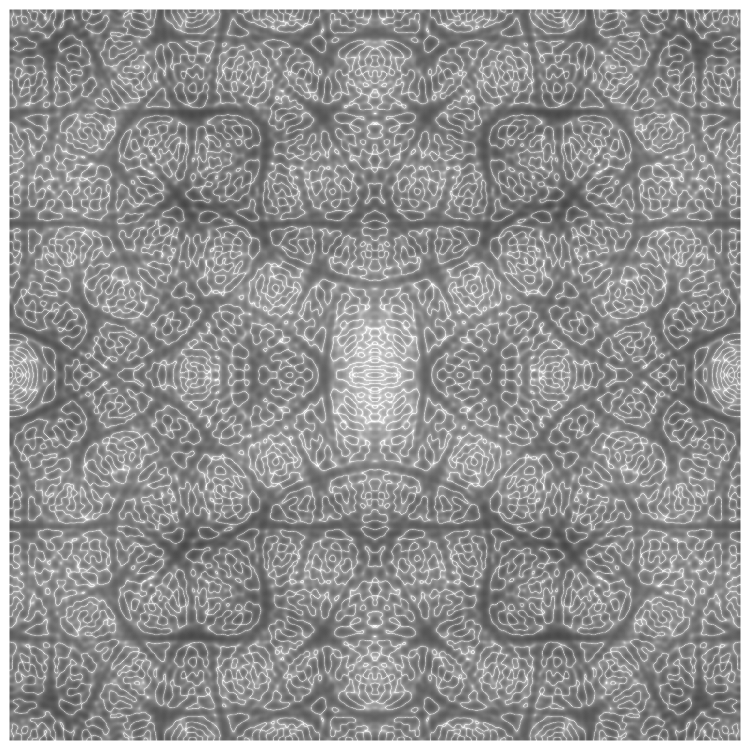
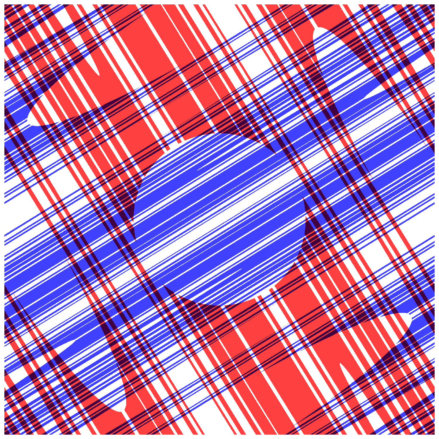
We remark that the conditions of Theorem 1 are always satisfied if (i.e. is a matrix) and is hyperbolic, that is it has no eigenvalues on the unit circle. Thus Theorem 1 (or more precisely, Theorem 2 below) implies the result of [Sch21]. See Figure 1 for a numerical illustration in the case . For , our assumption (1.3) does not require to be hyperbolic. We also remark that having characteristic polynomial irreducible over is a generic property for integer symplectic matrices, see Rivin [Riv08] and the book of Kowalski [Kow08, Theorem 7.12].
1.2. Further results
Theorem 1 is a consequence of a more general result, Theorem 2 below, that applies to quasimodes of and does not require the irreducibility over of the characteristic polynomial of . Before stating it, we need to introduce more notation. In order to measure the strength of a quasimode, we introduce for the quantity
| (1.5) |
where denotes the unit circle in . Note that if and only if is an eigenfunction of .
To relax the assumption on the characteristic polynomial of , let us notice that by (1.3) the leading eigenvalue is real. Since the matrix is symplectic, its transpose is conjugate to its inverse, thus is also a simple eigenvalue for and . Moreover, all other eigenvalues of satisfy .
Denote by the (real) eigenspaces of associated to . Let be the smallest subspace of such that is contained in . Note that are invariant under . Denote by
| (1.6) |
the subtori given by the projections of to .
The tori are relevant here because of their alternative dynamical definition given in Lemma 4.3: if is any eigenvector of associated to the eigenvalue , then the closure of the orbit of a point by the translation flow generated by is . In our setting, these translation flows will play the role that was played by the horocyclic flows on the unit tangent bundle of hyperbolic surfaces in [DJ18]. Let us also give
Definition 1.1.
Let and be respectively an open subset and a subtorus of and assume that . We say that satisfies the geometric control condition transversally to if, for every , there exists such that intersects .
We now state a more general version of Theorem 1:
Theorem 2.
Assume that satisfies (1.3). Let be such that satisfies the geometric control condition transversally to and . Then there exists such that for all large enough and every , we have
| (1.7) |
Theorem 2 implies Theorem 1. Indeed, if the characteristic polynomial of is irreducible over the rationals, then (see Lemma A.3), thus every nonempty open set satisfies the geometric control condition transversally to and . However, one can find a matrix that satisfies (1.3) but for which (1.4) fails for certain choices of (in particular the characteristic polynomial of is reducible over ) – see the examples in §A.2.
We will also prove the following theorem about damped quantum cat maps. It is analogous to exponential energy decay for negatively curved surfaces proved in [DJN22] (following earlier work of Jin [Jin20] in the constant curvature case):
Theorem 3.
Assume that satisfies (1.3). Let be such that . Assume that the set satisfies the geometric control condition transversally to and . Then there exists such that for all large enough the spectral radius of the operator is less than .
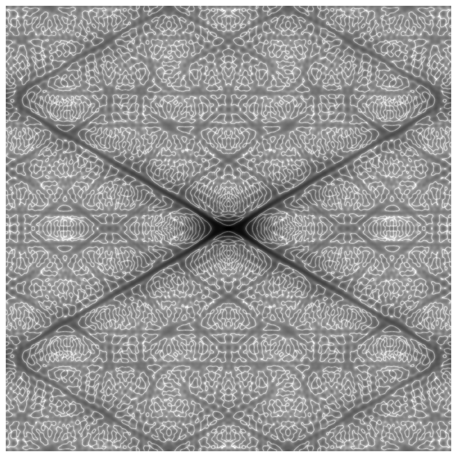
Note that by Lemma A.3, if the characteristic polynomial of is irreducible over then the condition on simplifies to . See Figure 2 for a numerical illustration.
1.3. Semiclassical measures and overview of history
We now give an application of Theorem 2 to semiclassical measures. These measures describe the possible ways in which the mass of eigenfunctions of can distribute in the position-frequency space in the limit , and they are defined as follows:
Definition 1.2.
Let , be sequences such that the quantization condition (2.57) holds for all . Let be eigenfunctions of of norm 1. We say that the sequence converges weakly to a Borel measure on if
| (1.8) |
A measure on is called a semiclassical measure (associated to the toric automorphism ) if there exist sequences such that (1.8) holds.
One can show (similarly to [Zwo12, Theorem 5.2] using a diagonal argument, the norm bound (2.51), Riesz representation theorem for the dual to , and the sharp Gårding inequality (2.48)) that each norm 1 sequence has a subsequence which has a weak limit in the sense of (1.8). Every semiclassical measure is a probability measure on (as follows from taking in (1.8) and using that ) which is invariant under the map (as follows from (1.2)). Semiclassical measures for quantum cat maps are analogous to those for Laplacian eigenfunctions on a Riemannian manifold , which are probability measures on the cosphere bundle invariant under the geodesic flow – see [Zwo12, Chapter 5] for more information.
As explained in §3.3, Theorem 2 implies the following property of the support of semiclassical measures:
Theorem 4.
Assume that satisfies (1.3) and is a semiclassical measure associated to . Then contains a set of the form or for some . In particular, if the characteristic polynomial of is irreducible over the rationals, then .
In Appendix A, we discuss the algebraic properties of the spaces and , and their implications in terms of the supports of semiclassical measures for . In particular, we give examples of the following situations:
-
•
the characteristic polynomial of is irreducible, and hence the semiclassical measures are fully supported;
-
•
, in which case there are semiclassical measures supported on translates of and due to [Kel10];
-
•
and there are semiclassical measures supported in and ;
-
•
but the supports of semiclassical measures (associated to a certain basis of eigenfunctions) are strictly larger than or .
The last two cases emphasize the fact that when , one has to study the action of on in order to refine the information on the support of semiclassical measures given by Theorem 4.
We now give a brief overview of history of semiclassical measures in quantum chaos, referring the reader to review articles by Marklof [Mar06], Sarnak [Sar11], Nonnenmacher [Non13], and Dyatlov [Dya21] for more information. In the setting of eigenfunctions of the Laplacian on compact negatively curved Riemannian manifolds, the Quantum Ergodicity theorem of Shnirelman [Shn74], Zelditch [Zel87], and Colin de Verdière [CdV85] states that a density 1 sequence of eigenfunctions equidistributes, i.e. converges to the Liouville measure in a way analogous to (1.8). The Quantum Unique Ergodicity conjecture of Rudnick–Sarnak [RS94] claims that the whole sequence of eigenfunctions equidistributes, i.e. the Liouville measure is the only semiclassical measure. It is open in general but known in the particular cases of arithmetic hyperbolic surfaces for joint eigenfunctions of the Laplacian and the Hecke operators, which are additional symmetries present in the arithmetic case – see Lindenstrauss [Lin06] and Brooks–Lindenstrauss [BL14].
The works of Anantharaman [Ana08], Anantharaman–Nonnenmacher [AN07b], Anantharaman–Koch–Nonnenmacher [AKN09], Rivière [Riv10b, Riv10a], and Anantharaman–Silberman [AS13] establish entropy bounds, which are positive lower bounds on the Kolmogorov–Sinaĭ entropy of semiclassical measures. As mentioned in the beginning of the introduction, in the setting of negatively curved surfaces the paper [DJN22] gives another restriction: all semiclassical measures have full support. In the case of hyperbolic surfaces this was previously proved by Dyatlov–Jin [DJ18].
The study of quantum cat maps, which is the setting of the present paper, goes back to the work of Hannay–Berry [HB80]. Bouzouina–De Bièvre [BDB96] proved the analogue of quantum ergodicity in this setting. Faure–Nonnenmacher–De Bièvre [FNDB03] constructed examples of semiclassical measures for 2-dimensional quantum cat maps which are not the Liouville measure; this contradicts the Quantum Unique Ergodicity conjecture for quantum cat maps but it does not contradict Theorem 1 since these measures were supported on the entire . Faure–Nonnenmacher [FN04], Brooks [Bro10], and Rivière [Riv11] established ‘entropy-like’ bounds on semiclassical measures; see also Anantharaman–Nonnenmacher [AN07a] and Gutkin [Gut10] for entropy bounds for other models of quantum maps. As mentioned above, Schwartz [Sch21] obtained Theorem 1 for 2-dimensional quantum cat maps.
Kurlberg–Rudnick [KR00] introduced the analogue of Hecke operators in the setting of 2-dimensional quantum cat maps. For the joint eigenfunctions of a quantum cat map and the Hecke operators (known as arithmetic eigenfunctions) they showed that Quantum Unique Ergodicity holds; see also Gurevich–Hadani [GH11]. This does not contradict the counterexample in [FNDB03] since the quantum cat maps used there have eigenvalues of high multiplicity.
In the setting of higher dimensional quantum cat maps which have an isotropic invariant rational subspace, Kelmer [Kel10] constructed examples of semiclassical measures (for arithmetic eigenfunctions) which are supported on proper submanifolds of . On the other hand, if there are no isotropic invariant rational subspaces, then [Kel10] gives Quantum Unique Ergodicity for arithmetic eigenfunctions. Compared to Theorem 4, the conclusion of [Kel10] is stronger than and the assumption is weaker than the characteristic polynomial of being irreducible over rationals (since [Kel10] only assumes that there are no isotropic invariant rational subspaces), however the result of [Kel10] only applies to arithmetic eigenfunctions. For a further discussion of the relation of our results with those of [Kel10], see Appendix A.
1.4. Outline of the proof
We now give an outline of the proof of Theorem 2. For simplicity we assume that the symbol satisfies , as well as the following stronger version of the geometric control condition: there exists an open set such that on and each shifted torus , intersects . We also assume that is large and is an eigenfunction of .
1.4.1. Reduction to the key estimate
Take the partition of unity on
| (1.9) |
Quantizing to pseudodifferential operators, we get the quantum partition of unity
For an operator on and an integer , define the conjugated operator
Since is an eigenfunction of the unitary operator , we have for all and
| (1.10) |
We will propagate up to time , where is chosen so that
| (1.11) |
and the constant is chosen later. We write a refined quantum partition of unity
| (1.12) |
Since , we have (see (2.51)), thus we can bound the norm of the product by 2. Applying the partition (1.12) to and using (1.10) with , we then get
| (1.13) |
The key component of the proof is the following estimate valid for the right choice of :
| (1.14) |
Here the exponent only depends on the matrix and the choice of the partition (1.9).
Together with (1.13), the key estimate (1.14) implies the following weaker version of Theorem 2:
| (1.15) |
To remove the prefactor, we revise the decomposition in the same way as in [DJ18, DJN22] (which in turn was inspired by [Ana08]), including more terms into and using that the norm bound in (1.14) (or rather, its slight generalization) is a negative power of . See §3.1.2 for details.
1.4.2. Microlocal structure of the propagated operators
We now give an outline of the proof of the estimate (1.14). To simplify the presentation, we assume the following stronger version of the gap condition (1.3):
| (1.16) |
Let be the one-dimensional eigenspaces of corresponding to and . We also define to be the sum of the generalized eigenspaces corresponding to all eigenvalues of other than . Then
By (1.16) we have the following norm bounds as :
| (1.17) |
Returning to the proof of (1.14), conjugating by we reduce it to the bound
We would like to write the operators as quantizations of some symbols. By the exact Egorov’s Theorem (1.2), we have for all . However, when is too large the derivatives of the symbols grow too fast with and the methods of semiclassical analysis no longer apply.
If , then by (1.17) the derivatives of in the eigendirection are bounded by but the derivatives along the complementary hyperplane are bounded by . Thus lies in the anisotropic symbol class , consisting of -dependent functions in such that each derivative along gives an growth and derivatives in other directions give an growth – see §§2.1.4,2.2.3 for details. In order for the standard properties of semiclassical quantization to hold, we need , that is
| (1.18) |
For such we can then show (see Lemma 3.11) that for any
Reversing the direction of propagation and replacing with , we similarly have
Then the key estimate (1.14) reduces to
| (1.19) |
The symbols lie in the classes for each but when they cannot be put in the same symbol calculus. This is important because otherwise the norm of would converge as to , which would be equal to 1 as long as contains at least one periodic trajectory of .
1.4.3. Applying the fractal uncertainty principle
Of course, just not being in the same symbol calculus does not give the bound (1.19). This is where the fractal uncertainty principle of [BD18] enters.
We first discuss the case , that is, the matrix has size . Then the fractal uncertainty principle shows the decay bound (1.19) if the sets are porous on scales to 1 in the sense of Definition 4.1 below, and . Here we think of as subsets of and are two linearly independent linear functionals. (The original result of [BD18] is stated in the particular case , and the general case follows via conjugation by a metaplectic transformation.)
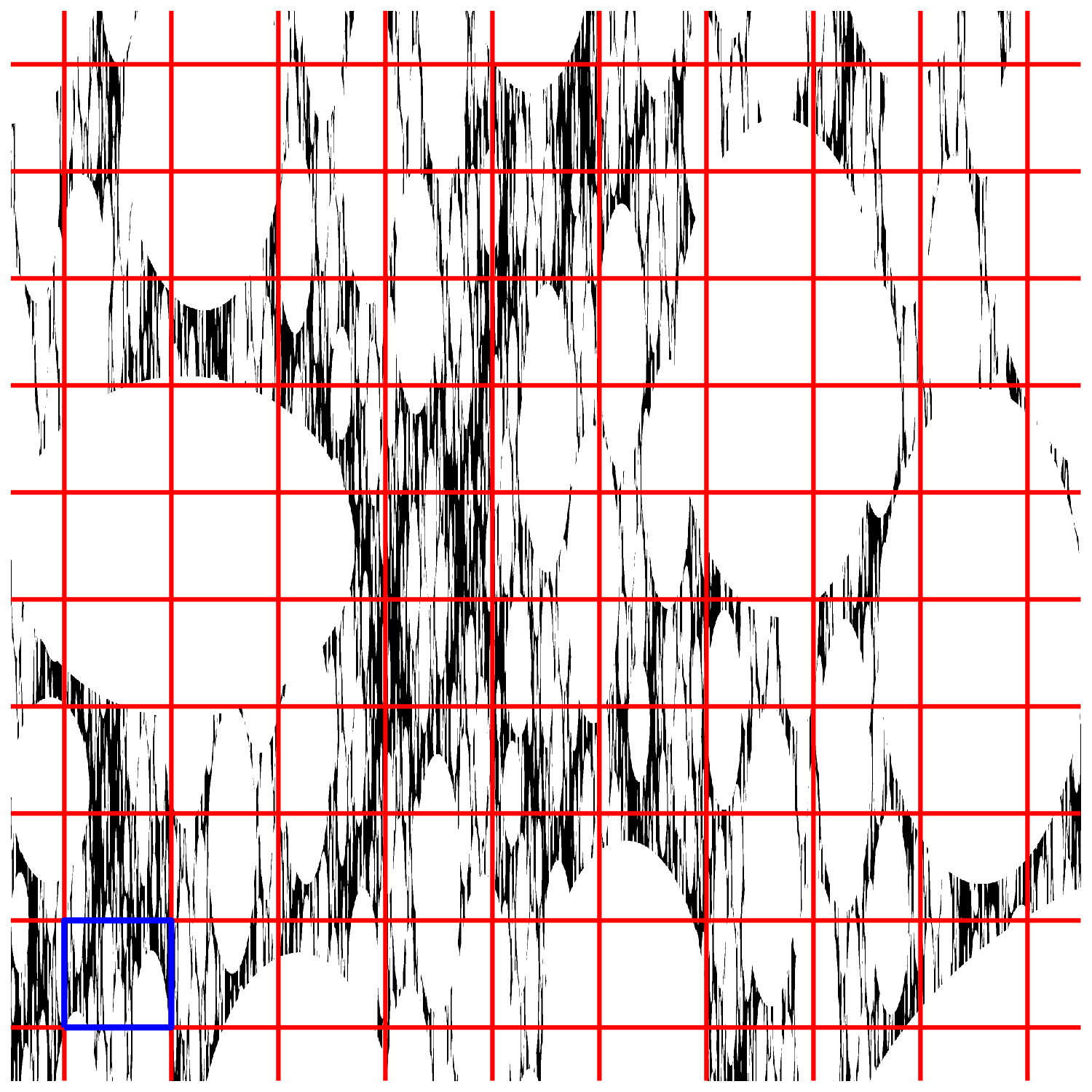
The required porosity property holds if we choose the projections such that their kernels are given by the eigenspaces . This is illustrated on Figure 3, and can be proved (taking the case of to fix notation) roughly speaking by combining the following observations:
-
(1)
Whether or not some belongs to depends on the forward trajectory , more specifically on whether the points in this trajectory all lie in .
-
(2)
The intersection of with any line in the direction is porous on scales to 1. Indeed, the projection of to is dense, so any sufficiently large line segment in the direction of intersects the complement of (recalling (1.9)). This creates the pores on scale 1. To get pores on smaller scales, we use that segments in the direction of are expanded by the map by the factor , so the condition that creates pores on scales .
-
(3)
If lie on the same line segment in the direction (of bounded length), then the forward trajectories , converge to each other as . Thus the projection looks similar to the intersection of with any fixed line segment in the direction of , which we already know is porous.
Now, if we take , then the fractal uncertainty principle applies and gives the key estimate. This roughly corresponds to the proof in [Sch21].
We now move on to the case of higher dimensions which is the main novelty of this paper. As mentioned above, the higher dimensional version of fractal uncertainty principle is not available. However, we can still derive the key estimate (1.19) from the one-dimensional fractal uncertainty principle as long as the projections are porous on scales to 1 for some , where are some fixed linear maps such that is a codimension 2 symplectic subspace of . Following the case , it is natural to take such that their kernels are given by the spaces . However, we cannot expect to be porous because the observation (3) above is no longer valid: there exist such that but as , for example one can take to be an eigenvector of with any eigenvalue such that .
To deal with this issue, we split the product of operators in (1.19) into a sum of many pieces:
| (1.20) |
where is a partition of unity on such that each looks like a ball of radius . We then observe that:
-
•
the terms in the sum in (1.20) form an almost orthogonal family, namely
This follows from the nonintersecting support property of semiclassical calculus, where we use that the symbols , grow by with each differentiation and thus belong to both the calculi where the symbols lie. By the Cotlar–Stein Theorem, this reduces the estimate (1.19) to a bound on the norms of the individual summands
(1.21) -
•
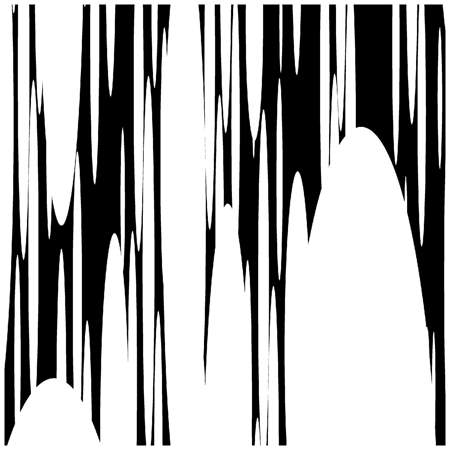
Each of the localized symbols does satisfy the porosity condition, namely is porous on scales to 1. This is because a localized version of the observation (3) above holds: if and has length , then for the difference is small. Indeed, by (1.16) the expansion rate of in the direction of is slower than , and . (See Figure 4.) On the other hand, an analogue of the observation (2) above holds as well: the closure of the projection of onto is equal to the subtorus , all of whose shifts intersect the complement of (see the beginning of §1.4). Thus the one-dimensional fractal uncertainty principle can be applied to give (1.21) and thus finish the proof.
In the above argument we again fix . More precisely we need so that the fractal uncertainty principle can be applied (i.e. we get porosity down to some scale below ), and we need so that semiclassical calculus could be used to get the almost orthogonality property.
There are several differences of the above outline from the actual proof of the key estimate. First of all, since we make the weaker spectral gap assumption (1.3) instead of (1.16), we need to revise the choice of and the parameters in the calculus – see §3.1.1. Secondly, at a certain point in the argument (see §3.5) we pass from the toric quantization to the Weyl quantization on , with .
1.5. Structure of the paper
-
•
In §2 we review semiclassical quantization and metaplectic operators on and on the torus , as well as the anisotropic symbol classes .
- •
- •
- •
Notation: if is a normed vector space and is a family depending on a parameter , then we say that if . We write if the constant in depends on some additional parameter(s) .
2. Preliminaries
2.1. Semiclassical quantization
Here we briefly review semiclassical quantization on , referring the reader to the book of Zworski [Zwo12] for details.
2.1.1. Basic properties
Let be the semiclassical parameter. Throughout the paper we denote by the Weyl quantization on . For a Schwartz class symbol it can be defined as follows [Zwo12, §4.1.1]:
| (2.1) |
One can extend this definition to belonging to the set of symbols (see [Zwo12, §4.4.1])
| (2.2) |
A natural set of seminorms on is given by
| (2.3) |
For any , the operator acts on the space of Schwartz functions and on the dual space of tempered distributions , see [Zwo12, Theorem 4.16].
We define the standard symplectic form on by
| (2.4) |
where denotes the Euclidean inner product on .
We now list several standard properties of the Weyl quantization:
-
•
Composition formula [Zwo12, Theorems 4.11–4.12, 4.17–4.18]: for
(2.5) the function is bounded in uniformly in and satisfies the following asymptotic expansion as for all :
(2.6) where is a second order differential operator in , . Each -seminorm of the remainder can be bounded by for some and depending only on .
-
•
Adjoint formula [Zwo12, Theorem 4.1]: if , then
(2.7) -
•
-boundedness [Zwo12, Theorem 4.23]: For , the operator is bounded uniformly in , more precisely its norm is bounded by for some depending only on .
-
•
Sharp Gårding inequality [Zwo12, Theorem 4.32]: if and for all , then
where the constant has the form for some depending only on .
The above properties imply in particular the nonintersecting support property
| (2.8) |
The next lemma gives an improved version of (2.8) in a special case when are separated far from each other in some direction. Lemma 2.1 is needed for the proof of Lemma 2.4, which is itself used in the proof of Lemma 4.5.
Lemma 2.1.
Let be a linear functional of norm 1 and assume that satisfy for some
| (2.9) |
Then for each we have
| (2.10) |
where the constant depends only on , , and some seminorms , where depends only on .
Proof.
If , then (2.10) follows immediately from (2.8). The constant does not depend on or : we only use that all the terms in the expansion (2.6) for are equal to 0. Thus we henceforth assume that .
1. Fix a function
Then there exists a constant such that
| (2.11) |
Now define the function
It follows from (2.11) that the function , as well as any its power , is an order function in the sense of [Zwo12, §4.4.1].
Following [Zwo12, (4.4.2)], we define for an order function the class of symbols consisting of functions satisfying the derivative bounds
The space has a natural family of seminorms defined similarly to (2.3).
2. Take arbitrary . From the support property (2.9) we see that
where the constants in depend only on some -seminorms of . The composition formula (2.6) is true for , with the remainder in the expansion still in , see [Zwo12, Theorems 4.17–4.18]. Since , all the terms in the asymptotic expansion (2.6) are zero, so in particular
Now (2.10) follows from the -boundedness property of quantizations of symbols in . ∎
2.1.2. Quantum translations
For , consider the operator
| (2.12) |
Here the symbol lies in , though its seminorms are not bounded uniformly in . By [Zwo12, Theorem 4.7] we have
| (2.13) |
In particular, is a unitary operator on .
We call a quantum translation because it satisfies the following exact Egorov’s Theorem (which is easy to check for using (2.1) and extends to the general case by density):
| (2.14) |
The map is not a group homomorphism, instead we have
| (2.15) |
This in particular implies the commutator formula
| (2.16) |
2.1.3. Metaplectic transformations
Denote by the group of real symplectic matrices, i.e. linear isomorphisms such that, with the symplectic form defined in (2.4),
For each , denote by the set of all unitary transformations satisfying the following exact Egorov’s theorem:
| (2.17) |
Such transformations exist and are unique up to multiplication by a unit complex number, see [Zwo12, Theorem 11.9]. Moreover, they act and . The set
is a subgroup of the group of unitary transformations of called the metaplectic group and the map is a group homomorphism .
The metaplectic transformations and the quantum translations are intertwined by the following corollary of (2.17):
| (2.18) |
2.1.4. Symbol calculus associated to a coisotropic space
We now introduce an exotic calculus corresponding to a linear foliation by coisotropic spaces. For each subspace , define its symplectic complement as
| (2.19) |
Note that is a subspace of dimension .
We call coisotropic if . This in particular implies that . The case corresponds to being Lagrangian, that is . On the opposite end, both the whole and any codimension 1 subspace of it are coisotropic.
Our exotic calculus will use symbols in the class , defined as follows:
Definition 2.2.
Let be a coisotropic subspace. Fix
We say that an -dependent symbol lies in if for any choice of constant vector fields on such that are tangent to there exists a constant such that for all
| (2.20) |
Remarks. 1. The derivative bounds (2.20) can be interpreted as follows: the symbol can grow by when differentiated along and by when differentiated in other directions.
2. If is Lagrangian, then a version of the class corresponding to compactly supported symbols but an arbitrary (not necessarily constant) Lagrangian foliation previously appeared in [DJ18] which inspired part of the argument in the present paper. In the important special case this class was introduced in [DZ16].
3. In the case the class does not depend on and becomes the standard mildly exotic pseudodifferential class , see [Zwo12, §4.4.1]. In particular, if then we recover the class defined in (2.2).
4. In [DZ16, DJ18] the value of was taken close to 1 and was either 0 or very small. In the present paper we choose in a more complicated way depending on the size of the spectral gap of the matrix , see §3.1.1.
Each lies in for any fixed value of . Therefore, the quantization defines an operator on . The -seminorms of are not bounded uniformly as , so the standard properties of quantization from §2.1.1 do not apply. However, using that and the fact that is coisotropic, we can establish analogues of these properties with weaker remainders:
Lemma 2.3.
1. Assume that . Then where satisfies the following asymptotic expansion as for all :
| (2.21) |
2. Assume that . Then is bounded uniformly in .
3. Assume that and everywhere. Then there exists a constant such that
| (2.22) |
The constants in the above estimates depend only on certain -seminorms of similarly to the properties of the -calculus in §2.1.1, where the choice of the seminorms additionally depends on .
Proof.
1. Let . Since is coisotropic, there exists a linear symplectomorphism
| (2.23) |
Denote where and . For , we have
where the space can be characterized by the following inequalities for all multiindices :
| (2.24) |
Fix a metaplectic operator . Then by (2.17) (which applies since the symbols in question are in for any fixed )
Since is unitary on and the terms in the expansion (2.21) are equivariant under composing with , we reduce the proof of the lemma to the case .
2. Henceforth we assume that . We use the unitary rescaling operator on defined by
A direct calculation using (2.1) shows that for all we have
| (2.25) |
By (2.24) we see that uniformly in . This gives parts 2–3 of the lemma.
3. To show part 1 of the lemma, define the symbol by the formula and consider the rescaling map . Then by (2.25)
| (2.26) |
Define the remainder
then by (2.26)
Since are bounded in uniformly in , we see from (2.6) with replaced by that
which implies that for all multiindices
| (2.27) |
If , i.e. is Lagrangian, then this immediately gives the expansion (2.21) as (2.27) shows that . In the general case, since we get that all the derivatives of the remainder become rapidly decaying in when , that is for each there exists such that . Combining this with the fact that the -th term in (2.21) is we see that the expansion (2.21) holds. ∎
Remark. Lemma 2.3 does not hold for the standard quantization
Indeed, consider the case and . The analog of the expansion (2.21) for the standard quantization is [Zwo12, Theorem 4.14]
Take and put for some nonzero -independent function . Then and the -th term in the asymptotic expansion for is
For , each successive term in the expansion grows faster in than the previous one, which makes it impossible for this expansion to hold. The difference between the standard and the Weyl quantization exploited in the proof of Lemma 2.3 is that the Weyl quantization obeys the exact Egorov Theorem (2.17) and the related fact that the terms in the asymptotic expansion (2.21) are equivariant under .
We also prove here a statement on composition of operators whose symbols have well-separated supports, used in the proof of Lemma 4.5:
Lemma 2.4.
Let be a linear functional of norm 1 and assume that satisfy for some and
| (2.28) |
Then for each and we have
| (2.29) |
where the constant depends only on , , and some -dependent -seminorms of .
Proof.
1. We first show that for all satisfying (2.28) and all
| (2.30) |
We may shift the supports of by conjugating by a quantum translation (see (2.14)), so we may assume that . We may also conjugate by a metaplectic transformation similarly to Step 1 in the proof of Lemma 2.3 to reduce to the case where is defined in (2.23). Next, using the dilation formula (2.25) we see that
where and the rescaled symbols , lie in uniformly in . The support condition (2.28) implies that
where we put
Note that and thus .
2. We now prove (2.29). If then (2.29) follows by applying twice the composition formula (2.21) and using the boundedness property of the class and the fact that . Henceforth we assume that . Fix
and decompose
Then the symbols are bounded in uniformly in . Moreover
We now write and estimate (using boundedness of , )
We finally use (2.30) with replaced by and replaced by to get
which finishes the proof. ∎
2.2. Quantization on the torus
In this section we study quantizations of functions on the torus
Each can be identified with a -periodic function on . This function lies in the symbol class defined in (2.2) and thus its Weyl quantization is an operator on . We will decompose into a direct integral of finite dimensional spaces , , which we call the spaces of quantum states. The operator descends to these spaces and gives a quantization of the observable . Our presentation partially follows [BDB96].
To make sure that the spaces of quantum states are nontrivial, we henceforth make the following assumption (see [BDB96, Proposition 2.1]):
| (2.31) |
2.2.1. The spaces of quantum states
Recall the quantum translations , , defined in §2.1.2. By (2.14) we have the commutation relations
| (2.32) |
This motivates the following definition of the spaces of quantum states: for each , put
| (2.33) |
where the quadratic form on is defined by
| (2.34) |
Denote
The following description of the spaces is a higher dimensional version of [BDB96, Proposition 2.1]:
Lemma 2.5.
The space is -dimensional with a basis given by , , where for we define
| (2.35) |
Remark. The distributions satisfy the identities
| (2.36) | ||||
In particular, even though the space is canonically defined for in the torus , in order to define the basis we need to fix a representative . Note also that is supported on the shifted lattice .
Proof.
By (2.16), for each the quantum translation is an isomorphism from onto . On the other hand, we compute for all and
| (2.37) |
Thus it suffices to consider the case .
Using and in the definition (2.33), as well as (2.15), we can characterize as the set of all such that
| (2.38) |
The first condition in (2.38) is equivalent to being a linear combination of delta functions at the points in the lattice , that is
The second condition in (2.38) is then equivalent to the periodic property for all . It follows that is the span of , which finishes the proof. ∎
We fix the inner product on each by requiring that be an orthonormal basis. Note that while the basis depends on the choice of the representative , the inner product only depends on as follows from (2.36).
Using the bases , we can consider the spaces as the fibers of a smooth -dimensional complex vector bundle over , which we denote by .
2.2.2. Decomposing
We now construct a unitary isomorphism between and the space of sections . This gives a decomposition of into the direct integral of the spaces over .
Define the operators by
| (2.39) |
Even though the basis depends on the choice of the preimage , the operator does not depend on this choice as follows from (2.36). We next define the operator
We also define the operator as follows: for
Here one can check that using a non-stationary phase argument and the following corollary of (2.36):
Lemma 2.6.
The map extends to a unitary isomorphism from to and extends to its adjoint.
Proof.
We argue similarly to [BDB96, Proposition 2.3].
1. We first show that extends to an isometry from to . For that it suffices to show the identity
| (2.40) |
For and , define the function by
Then can be written as a Fourier series:
Therefore by Parseval’s Theorem
We then have
which gives (2.40).
2. It remains to show that is onto and is the adjoint of . For that it suffices to prove that for each we have . We compute for all and
Here in the last line we use that by (2.36), as well as convergence of the Fourier series of the function . We now compute for all , finishing the proof. ∎
By duality, we may extend to operators
We then have the natural formula
| (2.41) |
which follows by duality from the identity
2.2.3. Semiclassical quantization
Fix and put as before. Let . By (2.32) and (2.33), the operator maps each of the spaces to itself. This defines the quantizations
which depend smoothly on .
A special case is given by which is independent of and -periodic in . In this case is the multiplication operator by (see [Zwo12, Theorem 4.3]), so by (2.35)
| (2.42) |
In particular, is the identity operator on .
Let be the unitary operators constructed in §2.2.2. By (2.41), they relate the operator to its restrictions as follows:
| (2.43) |
Notice that (2.43) may also be deduced from the explicit expression (verified by an explicit computation using (2.13), (2.35), (2.39), and the Poisson summation formula; the series below converges in )
| (2.44) |
and the commutation identity (2.32).
Since depends smoothly on , it follows from (2.43) and Lemma 2.6 that
| (2.45) |
Recall from Definition 2.2 the symbol class where is a coisotropic subspace and , . We similarly define the corresponding symbol class on the torus
whose elements are the -periodic symbols in . Note that putting we obtain the standard symbol class consisting of functions in with all derivatives bounded uniformly in .
Using (2.43) and (2.45), we see that Lemma 2.3 applies to the quantization . In particular, we have the product formula for all
| (2.46) |
where satisfies the expansion (2.21), the adjoint formula (following from (2.7))
| (2.47) |
the norm is bounded by some -seminorm of , and we have the sharp Gårding inequality for all such that everywhere
| (2.48) |
where is some -seminorm of . The choice of seminorms above depends on but not on or . The inequality (2.48) follows from the usual sharp Gårding inequality, and Lemma 2.6 that implies that is self-adjoint and that its spectrum is contained in the spectrum of .
We now give several corollaries of the basic calculus above. First of all, from (2.46), the expansion (2.21) with , and the boundeness of the operator norm of we get for all
| (2.49) |
where the constant in depends only on some -seminorms of .
Next, we have the following inequality of norms:
Lemma 2.7.
Assume that and everywhere. Then we have for all
| (2.50) |
where the constant depends only on some -seminorms of .
Remark. Taking to be the constant symbol , we get
| (2.51) |
where only depends on some -seminorm of .
Proof.
Finally, we record here the following lemma regarding products of many quantized observables, which is analogous to [DJ18, Lemmas A.1 and A.6]:
Lemma 2.8.
Assume that , where , satisfy and each -seminorm of is bounded uniformly in . Then:
1. The product lies in for all small .
2. We have for all
Here the constant in depends only on , and on the maximum over of a certain -seminorm of .
Proof.
1. We have , so it suffices to show that for each constant vector fields on such that are tangent to we have
| (2.54) |
Using the Leibniz Rule, we write as a sum of terms. Each of these is a product of the form where each is a product of some subset of and . Using that and each is bounded in uniformly in , we get (2.54).
2.2.4. Quantization of toric automorphisms
Let be the subgroup of integer symplectic matrices, i.e. elements of which preserve the lattice . We will quantize elements of as unitary operators on the spaces provided that satisfy the condition (2.57) below. To do this we need the following
Lemma 2.9.
Remark. Note that the map satisfies for all
Proof.
For , denote
We have
which together with the fact that implies that
Thus is a group homomorphism , which gives the existence and uniqueness of such that (2.55) holds. ∎
Now, fix and choose a metaplectic operator (see §2.1.3)
Here we put as before. Using (2.18) and (2.33) we see that
Denote
which depends smoothly on . Using (2.41) or (2.44), we see that the action of on is intertwined with the operators as follows:
| (2.56) |
Since is unitary on , it follows that each is a unitary operator as well.
We will be interested in the spectrum of , so we need its domain and range to be the same space . This is true if we choose such that the following quantization condition holds:
| (2.57) |
Note that when is even or , the equation (2.57) is satisfied in particular when .
2.2.5. Explicit formulas
Here we give some explicit formulas for the operators and . These are not used in the proofs but are helpful for implementing numerics. For simplicity we assume in this subsection that .
Our first statement computes the expression in terms of the values of at the points in the lattice . As before we define and similarly .
Proposition 2.10.
Let . Then for all we have
| (2.59) |
Proof.
Since trigonometric polynomials are dense in , it suffices to consider the case of
Using (2.12), (2.37), and (2.36), we compute for all
Therefore the left-hand side of (2.59) is
On the other hand, the right-hand side of (2.59) is equal to
The sum over is equal to 0 unless which happens for exactly one value of . Using that for this we write the right-hand side of (2.59) as
This equals the left-hand side of (2.59) which finishes the proof. ∎
We now compute the action of metaplectic transformations where for some and we assume that is even so that (2.57) is satisfied for and all . The general formulas are complicated, so instead we follow the approach of [Kel10, §1.2.1]. As proved for instance in [Koh97] the group is generated by matrices of the following block form, where denotes the transpose of :
| (2.61) | ||||
Since the map such that is a group homomorphism, it suffices to compute the operators for where is in one of the forms (2.61). This is done in
Proposition 2.11.
Assume that is even. Then there exist
| (2.62) | ||||
| (2.63) | ||||
| (2.64) |
for all and where .
3. Proofs of Theorems 2–4
In this section, we reduce the proofs of Theorems 2 and 3 to a decay statement for long words, Proposition 3.10, that will be proved in §4. In §3.1, we introduce notation that will be used in the proofs of Theorems 2 and 3 and state the main estimates that we will need to write these proofs: Lemmas 3.1, 3.2, and 3.4. In §3.2, we explain how these estimates allow us to prove Theorems 2 and 3. In §3.3, we derive Theorem 4 from Theorem 2. In §3.4, we prove Lemmas 3.1 and 3.2. Finally, in §3.5, we reduce Lemma 3.4 to Proposition 3.10.
Our strategy in this section generally follows [DJ18, Jin20, DJN22]. However, the proofs have to be modified to adapt to the setting of quantum maps used here and to the assumption of geometric control transversally to . Another important difference is the choice of propagation times, see §3.1.1.
Throughout this section we fix that satisfies the spectral gap condition (1.3) and choose a metaplectic operator quantizing . We take large and satisfying the quantization condition (2.57) and study the restrictions of to the spaces of quantum states , see §2.2.4. Following (2.31) we put .
3.1. Words decomposition
In the proofs of both Theorems 2 and 3, we will consider two -independent functions on the torus . The choice of these functions will differ in the proof of each theorem, but we will always assume that they satisfy
| (3.1) |
The functions and are supposed given for now, we will explain in the proofs of Theorems 2 and 3 how they are constructed. We will always explicitly point out when specific properties of and are required.
Let us write and take the quantizations (see §2.2.3)
For any operator on and , we define the conjugated operator
| (3.2) |
For , we introduce the set of words
For , define the operator
| (3.3) |
and the corresponding symbol
| (3.4) |
To a function , we associate the operator
| (3.5) |
and accordingly the symbol
If is the characteristic function of a subset , then we simply write instead of . Notice then that we have
| (3.6) |
In the proof of Theorem 2, we will have , and thus as well. On the other hand, Theorem 3 will be deduced from estimates on large powers of that will follow from estimates on for large.
3.1.1. Propagation times
We need now to fix a few parameters that will be used to choose a relevant value of . Recall from §1.2 that by the spectral gap assumption (1.3), has two particular simple eigenvalues
| (3.7) |
and all other eigenvalues of are contained in the open annulus . Fix a constant such that
Define the hyperplanes
| (3.8) |
Note that are coisotropic (since they have codimension 1), invariant under and, denoting by the eigenspaces of corresponding to ,
| (3.9) |
Moreover, since we have (where denotes the symplectic form from (2.4))
| (3.10) |
Next, is the sum of all generalized eigenspaces of with eigenvalues not equal to . Therefore we have the spectral radius bounds
| (3.11) | ||||
Let us now fix two numbers such that
| (3.12) |
We also fix an integer that satisfies
| (3.13) |
We now set
| (3.14) |
We call the short logarithmic propagation time and the long logarithmic propagation time.
Remark. Let us give some explanations regarding the choice of and the propagation times :
- •
- •
- •
- •
-
•
It is also useful to consider what happens in degenerate cases. Assume first that all the eigenvalues in lie on the unit circle (this is true in particular if ). Then we could take to be any fixed number in and to be any sufficiently small positive number. This is the choice made in [DJ18] (which additionally took close to 1).
-
•
On the other hand, if is close to (i.e. the spectral gap of is small) then our conditions force to both be close to .
3.1.2. Partition into controlled/uncontrolled words and main estimates
We now decompose the operator , , into the sum of two operators corresponding to the controlled and uncontrolled region (see (3.20) below), and state the main estimates used in the proofs of Theorems 2 and 3.
Let be the function that gives the proportion of the digit in a word, that is for we have
| (3.16) |
Let then be very small (small enough so that Lemma 3.4 below holds) and define
| (3.17) |
We call elements of controlled short logarithmic words.
We next use the set to split into two subsets: , writing each word in as a concatenation of words in :
| (3.18) | ||||
| (3.19) |
We call elements of uncontrolled long logarithmic words and elements of controlled long logarithmic words.
It follows from (3.6) that (with the operators defined using (3.5))
| (3.20) |
In order to get an estimate on , we will control and separately. Let us start with . It will be dealt with differently in the proofs of Theorem 2 and 3, but the main idea is the same: we make an assumption on the symbol that translates into control on the operator that is inherited by . In more practical terms, we will use the following lemma in the proof of Theorem 2.
Lemma 3.1.
Let . Assume that satisfy
| (3.21) |
Let . Then there is a constant such that for all and
| (3.22) |
Here we recall that the quantity , defined in (1.5), measures how close is to an eigenfunction of . Note that the condition (3.13) on ensures that the power of in the last term on the right-hand side of (3.22) is negative for small enough.
Lemma 3.2.
The control on will be more subtle to obtain. We will use the following estimate, whose proof ultimately relies on the Fractal Uncertainty Principle. Recall the subtori defined in (1.6), and make the following
Definition 3.3.
Let be a set. We say that is safe if and only if for every , each of the shifted tori , intersects .
Notice that being safe is slightly more restrictive than satisfying the geometric control condition with respect to and (Definition 1.1) as we do not have here the flexibility to replace a point by its image by an iterate of .
The control on is achieved in
Lemma 3.4.
3.2. Proofs of Theorems 2 and 3
Let us explain now how Lemmas 3.1–3.4 allow us to prove Theorems 2 and 3. First of all, we need to construct the functions and that appear in the statement of these lemmas. To do so, we will use the following two lemmas:
Lemma 3.5.
Assume that is a safe open set. Then contains a safe compact subset .
Proof.
We argue by contradiction: we write where are compact sets with and assume that none of the ’s are safe. Then for every there exist
Up to extracting a subsequence, we may assume that is constant equal to some and that converges to some point . Since is safe, the set intersects . Take and put . Then , so for large enough. This gives a contradiction with our assumption that does not intersect . ∎
Lemma 3.6.
Let be an open subset of which is safe in the sense of Definition 3.3. Then there exist such that
and the complements , are both safe.
Proof.
1. We show that there exist two compact sets
| (3.25) |
and are both safe. To do this, let be a hyperplane transverse to each of the tangent spaces of where are the subspaces defined in the paragraph preceding (1.6). Denote by the projection map. Take large , denote by the closed ball of radius in , and define
Then, we can fix large enough so that the set is safe. Indeed, every element of can be written as for some . Then we can decompose where , . Moreover, if is large enough then we can choose this decomposition so that . Then .
Now, the open set is safe since is open and safe and each intersection has empty interior in . Then by Lemma 3.5 there exists a safe compact set . The complement contains and thus is an open safe set. Using Lemma 3.5 again, let be a compact safe subset of this complement, then satisfy (3.25).
2. Using a partition of unity subordinate to the cover of by the sets , we choose such that
The complements of , contain the sets , and are thus both safe, finishing the proof. ∎
Proof of Theorem 2.
Let be as in the statement of Theorem 2. Since satisfies the geometric control condition transversally to and , the open set
is safe. We apply Lemma 3.6 to to construct two functions and we set and in §3.1. Notice that we have consequently and (3.20) becomes
Fix be small enough so that Lemma 3.4 applies, that is there are such that for every we have
| (3.26) |
Next, applying Lemma 3.1 with sufficiently small , recalling (3.13), and making larger and smaller if needed, we have for every
| (3.27) |
Putting (3.26) and (3.27) together, we find that, for every , we have
| (3.28) |
Now, for large enough we can remove the last term on the right-hand side of (3.28), obtaining (1.7) and finishing the proof.∎
Proof of Theorem 3.
We will find -independent constants and an integer such that
| (3.29) |
It will then follow from (3.29) that the spectral radius of is bounded above by
which will give the conclusion of the theorem.
1. We first reduce to the situation when the set is safe (which is a stronger assumption than made in Theorem 3). Consider the open set
By the assumption of the theorem, the set is safe. By Lemma 3.5, contains a safe compact subset . Since each is open, we may fix such that , which implies that is safe.
Using (2.51) to bound the operator norm of by , we have for any fixed
Hence to show (3.29) it suffices to prove
| (3.30) |
The operator lies in , with the matrix still satisfying the spectral gap assumption (1.3) and producing the same tori . Therefore, to show (3.30) it suffices to prove the bound
| (3.31) |
for any satisfying (1.3) and any , where we assume that , everywhere, and the set is safe.
2. We now show (3.31). Using Lemma 3.6 for the set , we construct two cutoff functions . Put
Note that in agreement with the convention of §3.1 and . Moreover, . By construction, and satisfy the hypotheses of Lemma 3.4. Consequently, we can choose small enough so that this lemma applies: there are such that
As is supported in , we see that on , and we can consequently apply Lemma 3.2 to see that, up to making larger and smaller, we also have
Recalling (3.20), we see that
Since is defined by (3.14), we just established (3.31), which ends the proof of the theorem. ∎
3.3. Proof of Theorem 4
We argue by contradiction. Let be a semiclassical measure associated to and assume that does not contain any sets of the form or . Then the complement is an open safe set in the sense of Definition 3.3. By Lemma 3.5, there exists a compact safe set such that . Take such that and on . Then the set is safe, so satisfies the hypothesis of Theorem 2.
Let be a sequence converging to in the sense of (1.8). Since is an eigenfunction of and , Theorem 2 shows that there exists a constant such that for all large enough
| (3.32) |
Now, by (2.47) and (2.49) (with ) we have
| (3.33) | ||||
By (3.32), the left-hand side of (3.33) is bounded away from 0 as . By (1.8), the right-hand side of (3.33) converges to ; thus this integral is positive. This contradicts the fact that and finishes the proof.
3.4. Estimates in the controlled region
Here we prove Lemmas 3.1 and 3.2, using the notation that we introduced in §3.1. We start by relating the operator from (3.3) and the symbol from (3.4). Recall the symbol classes from §2.2.3, the constants defined in (3.12), the integers defined in (3.13) and (3.14), and the hyperplane defined in (3.8).
Lemma 3.7.
Let . For every , the symbol belongs to the symbol class and
Here the semi-norms of and the constant in the are bounded uniformly in .
Proof.
1. We first show that each -seminorm of the symbols
is bounded uniformly in and . To simplify notation we give the proof for , which applies to as well (in fact, it applies with replaced by any fixed function in ).
Let be constant vector fields on such that are tangent to . Since is a linear map, we compute for
Here, denotes the -th derivative of , which is a -linear form, uniformly bounded since it does not depend on . Consequently, for some -independent constant , we have
Using the norm bounds (3.11) on and we get (for a different choice of )
which is precisely the required estimate. Here we used the definition (3.14) of and the condition (3.12) that we imposed on .
Proof of Lemma 3.2.
1. Let us prove first the required estimate for the operator (instead of ) associated to the set defined by (3.17). Put
then everywhere. For , denote
Recalling the function from (3.16) and the definition (3.4) of , we see that
Summing over , we find that
Let be very small. By (3.14), there are at most elements in . It follows from Lemma 3.7 that is bounded in uniformly in and that
We can consequently apply (2.51) to the symbol in order to find that, for some that may vary from one line to another,
| (3.34) |
with
Notice that the condition (3.13) that we imposed on ensures that is positive (provided is small enough).
2. The same proof with replaced by gives
| (3.35) |
3. Let us now use the estimates (3.34) and (3.35) to prove the lemma. If is the concatenation of the words , then by (3.3) we have
Using the definition (3.19) of , and splitting this set into the disjoint union of subsets corresponding to the largest such that , we write
| (3.36) |
According to (3.34) and (3.35), the operator norm of each term in this sum is less than
Since the number of terms in this sum is , that does not depend on , the estimate (3.24) follows. ∎
In order to prove Lemma 3.1, we need a few more preliminary results. We start with a norm estimate on the operators defined in (3.5).
Lemma 3.8.
Assume that . Let . Let
Then there is a constant , that does not depend on nor such that, for every , we have
Proof.
We will also use a standard elliptic estimate.
Lemma 3.9.
Let and assume that
Then there is a constant such that, for every and every , we have (with defined in (1.5))
| (3.37) |
Proof.
1. First of all, we may assume that everywhere, since we may replace with and use the following corollary of (2.49) (with ):
Here denotes an -independent constant whose precise value may change from line to line.
2. By a compactness argument, we see that there exists such that
We write for some . Then by (2.49) and (2.58)
Applying this with replaced by , we see that for all , with the constant independent of ,
| (3.38) |
3. We have for every operator , , and
| (3.39) |
Indeed, take such that . Then we have when ,
By a similar computation, we see that this estimate still holds when . These estimates imply (3.39).
We are now ready to prove Lemma 3.1.
Proof of Lemma 3.1.
We will prove the estimate (3.22) first for , then for , and finally for .
1. We start by considering the operator associated to the function defined by (3.16). Notice that the assumption that implies that for . It follows from the definition of that
Consequently, using Lemma 3.9, we find that for we have
Recalling the definition (3.14) of , we find that, up to making larger, we have
| (3.40) |
3.5. Reduction to a fractal uncertainty principle
We now explain how Lemma 3.4 may be deduced from a Fractal Uncertainty Principle type statement, Proposition 3.10 below. The proof of Proposition 3.10 is given in §4.3.
Let . Decompose the word into two words of length :
Then, we relabel and as
and define the symbols
| (3.43) |
In §4, we will prove the following estimate, where , is the Weyl quantization on defined in (2.1), and we treat as -periodic functions in .
Proposition 3.10.
Assume that the complements , are both safe in the sense of Definition 3.3. Then there are constants that do not depend on nor such that
In order to take advantage of Proposition 3.10, let us first notice that the proof of Lemma 3.7 also gives without major modification:
Lemma 3.11.
Let . The symbols and belong respectively to the symbol classes and , with bounds on the semi-norms that do not depend on . (Here are defined in (3.8).) Moreover, we have
where the constants in are uniform in .
Lemma 3.12.
Assume that the complements , are both safe. Then there are constants that do not depend on nor such that
Proof.
We start by noticing that
| (3.44) |
By Lemma 3.11, the operators are bounded in norm uniformly in . Hence, we deduce from Lemma 3.11 and (3.44) that, for some , we have
Now, we deduce from (2.43) that for every we have
Hence, using Lemma 2.6, we find as we did for (2.45) that
and the result follows then immediately from Proposition 3.10. ∎
In order to get an estimate on the operator norm of from Lemma 3.12, we will need the following bound on the cardinal of .
Lemma 3.13.
There are a constant (that does not depend on ) and a constant (that may depend on ) such that for large enough we have
Proof.
We have now all the tools required to prove Lemma 3.4.
4. Decay for long words
In this section, we use the fractal uncertainty principle, Proposition 4.2 below, to prove Proposition 3.10 and end the proof of Theorems 2 and 3. In §4.1, we recall the definition of porosity and the statement of the fractal uncertainty principle. In §4.2, we establish porosity estimates for the supports of and from Proposition 3.10, which allows us to use the fractal uncertainty principle in §4.3 to prove Proposition 3.10.
4.1. Fractal uncertainty principle
The central tool of our proof is the fractal uncertainty principle, due originally to Bourgain–Dyatlov [BD18]. Roughly speaking, it states that a function in cannot be localized in both position and (semiclassically rescaled) frequency near a fractal set. To make the statement precise, we use the following
Definition 4.1.
Let and be nonnegative real numbers. Let be a subset of . We say that is -porous on scales to if for every interval of length , there is a subinterval of length such that .
We also recall the definition of the -dimensional semiclassical Fourier transform:
| (4.1) |
Denote by the multiplication operator by the indicator function of . We use the following extension of the fractal uncertainty principle of [BD18] proved by Dyatlov–Jin–Nonnenmacher [DJN22, Proposition 2.10] (where we put , in the notation of [DJN22]):
Proposition 4.2.
Let and . Then there exist such that for every and every which are -porous on scales to , we have
Remark. The condition that is essential. Indeed, the sets are -porous on scales to 1, but does not go to 0 as , as can be checked by applying the operator in question to the function where has norm 1.
4.2. Porosity property
In order to use Proposition 4.2, we need to establish certain porosity properties for sets related to the support of and from Proposition 3.10. Recall that the symbols are defined in (3.43) using arbitrary words , where the long logarithmic propagation time is defined in (3.14). The functions used in the definitions of satisfy (3.1) and the complements , are both safe in the sense of Definition 3.3.
Fix eigenvectors of associated to the eigenvalues (see (3.7)). Note that by (3.9) and (3.10) we have . We choose so that we get the following identity used in §4.3.3 below:
| (4.2) |
We let be the translation flows on the torus corresponding to , that is
| (4.3) |
Recall that the subtori are defined as the projections to of the spaces where are minimal subspaces such that .
Lemma 4.3.
Let . Then the closure in of the orbit of under is
| (4.4) |
Proof.
Let us consider for instance the case of . By (4.3), it suffices to show that where
Since , we have , and let us prove the reciprocal inclusion.
The set is a closed subgroup of , thus it is a Lie subgroup. Let be the Lie algebra of ; since is connected, the exponential map is onto and thus where . Since is compact, the rank of the lattice is equal to the dimension of , thus where is the subspace generated by . Since , by the definition of we have . This implies that and thus as needed. ∎
We now fix a constant (to be chosen in Step 2 of the proof of Lemma 4.6 in §4.3.3 below) and introduce for the -dependent sets
| (4.5) |
Here as before; and have been introduced in §3.1.1, see in particular (3.8) and (3.12). We can visualize the sets as follows: let us lift to a subset of and to a point in . The set
is a cylinder in , and is the projection onto the direction of the intersection of this cylinder with .
The porosity statement needed in order to apply Proposition 4.2 is the following
Lemma 4.4.
Let . Then there exist , independent of such that, if , then for every , the sets and are -porous on scales to .
Remarks. 1. Lemma 4.4 is where we use the assumption that the complements , are both safe.
2. The choice of scales in Lemma 4.4 can be explained as follows using (3.15) (taking to simplify notation). On one hand, since , the map expands the vector by . Thus we expect porosity of in the direction of on scales from to 1. On the other hand, by (3.11), the same map sends the ball to a set of diameter , so changing by an element of this ball does not change much the forward trajectory under up to time , which is used to define the symbol in (3.43).
Proof.
We show the porosity of , with the case of handled similarly (reversing the direction of time).
1. Since the complements , are safe, by Lemma 3.5 there exist compact subsets such that the interiors are safe and
We claim that there exist constants , such that for any , the intersection of every length flow line of with contains a segment of length . (Here the length of flow lines is defined using the parametrization by .)
We argue by contradiction: assume that such do not exist, then there is a sequence such that for each the intersection does not contain any segment of length . Passing to a subsequence, we may assume that the sequence converges to some as . Since the interior is safe, it intersects . Then by Lemma 4.3 there exists such that . For large enough the segment lies inside . This contradicts our assumption and proves the claim.
2. Let . We will show that is -porous on scales to 1 for
Let be an interval of length between and . Let denote the smallest integer such that . By the definition (3.14) of , and recalling that ,
thus , provided is small enough.
Since , the set is a flow line of of length . Consequently, the intersection of this set with contains a segment of length . It follows that there exists a segment of length such that
| (4.6) |
By our choice of , we have . It remains to prove that . Recalling the definition (4.5) of , we see that it suffices to show that for each we have
We have . Recalling the bound (3.11) on the norm of restricted to , as well as the condition (3.12) we imposed on , we see that (with the constant depending on )
By (4.6) and since , we see that , provided is small enough so that is less than the distance between and . Recalling the definition (3.43) of , it follows that , which finishes the proof. ∎
4.3. Proof of Proposition 3.10
We now give the proof of Proposition 3.10, relying on the following three ingredients:
-
•
the fact that for any , we have uniformly in and in the words (see Lemma 3.11);
-
•
the porosity property of the supports given by Lemma 4.4;
-
•
and the fractal uncertainty princple in the form of Proposition 4.2.
Henceforth we treat as -invariant symbols in . All the constants in the estimates below are independent of .
4.3.1. Decomposing the operator and the scheme of the proof
We start by decomposing the operator into a series, see (4.8) below. For that, fix a function
For instance, we can start with such that the -periodic function is everywhere positive, and put .
Now, consider the partition of unity where the -dependent symbol is given by
| (4.7) |
Recalling Definition 2.2, we see that lies in uniformly in for any coisotropic subspace .
We have the following decomposition, with the series below converging in the strong operator topology as an operator , which can be checked by applying it to a function in :
| (4.8) |
We now state two estimates on the operators which together will give Proposition 3.10. The first one is an almost orthogonality type statement when is sufficiently large:
Lemma 4.5.
For every there exists a constant such that for every such that we have
The second one is the norm bound on each individual , which uses the fractal uncertainty principle:
Lemma 4.6.
There exist constants such that for every we have
Here the constant only depends on the porosity constant in Lemma 4.4 and on .
4.3.2. Almost orthogonality
Proof of Lemma 4.5.
1. Let be such that . Define the linear functional by
Note that has norm 1. Putting , we have
| (4.9) | ||||
Indeed, assume that . Then . Since and , we have . This gives the first statement in (4.9), with the second one proved similarly. Note that (4.9) implies in particular that .
2. We estimate the norm , with estimated in a similar way. We write using (2.5) and (2.7)
It follows from Lemmas 2.3 and 3.11 that is uniformly bounded on . Thus it suffices to show that
| (4.10) |
To show (4.10), it suffices to apply Lemma 2.4 with
Here for each the symbols are bounded in the class uniformly in by Lemmas 2.3 and 3.11, as well as (4.7). The support condition of Lemma 2.4 is satisfied by (4.9). ∎
4.3.3. Decay for an individual summand
Finally, we apply the fractal uncertainty principle to prove Lemma 4.6.
Proof of Lemma 4.6.
1. Recall that the ’s belong uniformly to both the symbol classes and . Recalling Lemma 3.11, we can apply the product formula from Lemma 2.3 to find that for every
Therefore it suffices to show that
| (4.11) |
2. We next study the supports of the symbols . We have from (4.7)
Thus by (3.9) any can be written as where , , and for some constant depending only on the matrix . Choose such that . Put . Recalling the definition (4.5) of the sets , we get
| (4.12) |
3. We now conjugate by a metaplectic transformation which ‘straightens out’ the vectors and the subspaces . Using (3.10), (4.2), and the linear version of Darboux’s Theorem, we construct a symplectic matrix such that
-
•
and ;
-
•
;
-
•
.
Let be a metaplectic operator associated to (see §2.1.3). Then by (2.17)
Thus (4.11) reduces to
| (4.13) |
and the support condition (4.12) becomes
| (4.14) | ||||
4. For , denote the -neighborhood of by
Let be the convolutions of the indicator functions of with the function where is a nonnegative function integrating to 1. Then
and for each there exists a constant (depending only on and the choice of ) such that
Define the symbols by
Then lie in the symbol class uniformly in . On the other hand, by Lemma 3.11 the symbols lie in the larger class uniformly in for every fixed . By Lemma 2.3 and since by (4.14), we have
Note that is a multiplication operator and is a Fourier multiplier (see [Zwo12, Theorem 4.9]). Multiplying the above estimates and using that are bounded uniformly as operators on , we reduce (4.13) to the following estimate:
| (4.15) |
5. If we consider as the Hilbert tensor product corresponding to the decomposition , , then the operators and are the tensor products of the same operators in one variable with the identity operator on . Thus (4.15) is equivalent to
| (4.16) |
where we now treat the factors in the product as operators on . Denote by the unitary semiclassical Fourier transform, see (4.1). Then . Thus the left-hand side of (4.16) is equal to . Since and , the bound (4.16) reduces to
| (4.17) |
6. We finally apply the fractal uncertainty principle. Fix , which is possible since by (3.12). By Lemma 4.4, there exists such that the sets are -porous on scales to 1. Since for , the neighborhoods are -porous on scales to 1 – see for example [DJN22, Lemma 2.11]. Now (4.17) follows from the fractal uncertainty principle of Proposition 4.2, and the proof is finished. ∎
Appendix A Properties of integer symplectic matrices
In this Appendix, we discuss the algebraic hypotheses made on the matrix in Theorems 2, 3, and 4. More precisely, we investigate the spaces and (and hence the tori and ) defined in (1.6). In particular, we prove Lemma A.3 that allows us to deduce Theorem 1 from Theorem 2.
A.1. Algebraic considerations
We start by giving a new characterization of and . Let satisfy the spectral gap condition (1.3) and recall from the introduction that were defined as the smallest subspaces of such that where are the eigenspaces of corresponding to the eigenvalues and .
We will be using basic field theory, see e.g. [DF04, Chapter 13]. Recall that for an algebraic number , its minimal polynomial (over ) is the unique irreducible monic polynomial such that . Two algebraic numbers are called Galois conjugates if they have the same minimal polynomial.
Lemma A.1.
Let denote the minimal polynomials of . Then . The dimensions of are equal to each other and to the degrees of . Moreover, we have the following two cases:
-
(1)
if is a Galois conjugate of , then ;
-
(2)
otherwise .
Proof.
1. We first show that and . (The case of is treated similarly.) Note that is an -invariant subspace of . Any (complex) eigenvalue of the endomorphism has to be a root of , thus the characteristic polynomial of is a power of . On the other hand, divides the characteristic polynomial of . Since is a simple eigenvalue of , we see that .
Since , we see that , and consequently we have . As is -invariant, the characteristic polynomial of the endomorphism divides the characteristic polynomial of the endomorphism . Since is irreducible over and , we see that these two characteristic polynomials are equal. It follows that and .
2. Recall that the degree of is the dimension of the field as a vector field over . Since , we have , so that . It follows that .
3. Since and are irreducible over the rationals, either they are coprime, in which case , or they are equal, in which case , due to the characterization we just proved. If , then and is a Galois conjugate of . Reciprocally, if , then and are not coprime, so that . ∎
In order to discuss the sharpness of Theorem 4, we introduce a decomposition of . For a subspace , denote by its symplectic complement, see (2.19). Recall that is called symplectic if .
Lemma A.2.
We have the following two cases:
-
(1)
if is a Galois conjugate of , then is symplectic;
-
(2)
otherwise are both isotropic and the symplectic form is nondegenerate on .
Consequently, we have a decomposition of into
where and are symplectic.
Proof.
1. For each complex eigenvalue , define the space of generalized eigenvectors
Then we have the decomposition
| (A.1) |
We claim that for all such that ,
| (A.2) |
To prove (A.2), we argue by induction on where are the smallest numbers such that . If or , then since or . Otherwise we use that is symplectic to write
Using the inductive hypothesis we see that the last two terms on the right-hand side are 0, which gives as needed.
2. Since is a simple eigenvalue of and is its minimal polynomial, each root of is a simple eigenvalue of . By Lemma A.1 we have
Since are the minimal polynomials of and , we have for some . It follows from (A.3) that
If is a Galois conjugate of , then , so is symplectic. Otherwise and are coprime, so are both isotropic and is nondegenerate on . ∎
Remark. Using Lemma 4.3, the algebraic consideration from this section have dynamical implication. Lemma A.1 that if then the closure of the orbits of for the flows and are either identical (if is a Galois conjugate of ) or have a finite number of points of intersection.
From Lemma A.2, we know that if then the closure of the orbit of under the action by translation of the -dimensional vector space generated by and is always a symplectic subtorus of .
A.2. Most favorable cases
Theorem 4 gives a condition on the support of semiclassical measures for in terms of the spaces and . The larger these spaces are, the stronger the conclusion of Theorem 4 is. Considering the decomposition from Lemma A.2, the most favorable case is when is trivial. In that situation, there are still two possibilities according to Lemma A.1:
-
(1)
, or
-
(2)
and are Lagrangian.
In case (1), Theorem 4 says that all semiclassical measures for are fully supported. Actually, this is exactly the setting of Theorem 1, as we prove now.
Lemma A.3.
The characteristic polynomial of is irreducible over if and only if (that is , or equivalently the flows and are minimal).
Proof.
Notice that divides the characteristic polynomial of and recall that the dimension of is the degree of . Hence, if is equal to , the degree of is and must be the characteristic polynomial of , which is consequently irreducible. Reciprocally, if the characteristic polynomial of is irreducible, it must be equal to , so that . ∎
Of course, when , the control of the support of semiclassical measures for given by Theorem 4 is sharp. When , satisfies the spectral gap condition (1.3) if and only if it is hyperbolic (i.e. it has no eigenvalues on the unit circle), and in this case we always have . When , one can easily construct examples of matrices satisfying (1.3) with irreducible characteristic polynomials. For example, when one can take
| (A.4) |
with the characteristic polynomial
which has a root in , a root in , and two complex roots on the unit circle.
Let us now consider the case (2), when . Our result is still sharp in this situation since, under some mild additional assumptions, Kelmer [Kel10, Theorem 1] constructed semiclassical measures supported in some translate of and semiclassical measures supported in some translate of . A basic example (previously presented by Gurevich [Gur05] and Kelmer [Kel10]) is
| (A.5) |
where , , has irreducible characteristic polynomial and a leading simple eigenvalue, that also dominates the inverses of the eigenvalues of (so that satisfies the spectral gap condition (1.3)). One can take for instance
Using the coordinates on , we see that the spaces are given by , . Note that if we allow to be in , then, when , the matrix is always of the form (A.5) after a symplectic (rational) change of coordinates.
Using Proposition 2.11, we see that for a matrix of the form (A.5) and , the following elements of are eigenvectors for the quantizations of :
It follows from Proposition 2.10 that these eigenvectors converge respectively to the semiclassical measures
These measures are supported respectively in and .
A.3. General case
For now, we only considered the case in which the space from Lemma A.2 is trivial. Let us now discuss what happens when is non-trivial. Let and be the subtori of tangent respectively to and . As before, we consider two cases:
-
(1)
If is a Galois conjugate of , then Theorem 4 shows that the support of every semiclassical measure contains a translate of .
-
(2)
Otherwise Theorem 4 shows that the support of every semiclassical measure contains a translate of or , which are different tori (their tangent spaces intersect trivially). On the other hand, from [Kel10, Theorem 1], we know that (under mild additional assumptions) there are semiclassical measures supported in some translate of and semiclassical measures supported in some translate of .
Note that in both cases the conclusion of Theorem 4 is not sharp. However, we cannot say more on the support of the semiclassical measures for without further information on the action of on .
To illustrate this fact, take a matrix that satisfies (1.3) and a matrix whose eigenvalues are dominated by the leading eigenvalue of . Assume in addition that in the decomposition from Lemma A.2 for the matrix , the factor is trivial. Then, we form the matrix
Notice that the matrix satisfies the condition (1.3) and that the action of on the spaces and is given respectively by the matrices and . The quantizations of are tensor products of quantizations of with quantizations of , with a basis of eigenfunctions consisting of tensor products of eigenfunctions corresponding to with those corresponding to . The torus decomposed as and the semiclassical measures for associated to eigenfunctions of product type are of the form where and are semiclassical measures respectively for and . We know that the support of must contain a translate of or (and this estimate cannot be improved as discussed in §A.2).
If the semiclassical measures for have large supports, then Theorem 4 is not sharp. For instance, if satisfies (1.3) and has an irreducible characteristic polynomial over the rationals, then must be fully supported, so that the supports of the semiclassical measures for (associated to eigenfunctions of product type) contain a translate of or .
However, it is not true in general that the semiclassical measures for have a large support. The most extreme case is when is given by the symplectic rotation matrix from (2.61). In that case, the Dirac mass at is a semiclassical measure for (as proved in Lemma A.4 below). Hence, all the measures of the form are semiclassical measures for , and we see that Theorem 4 is sharp in that case. A concrete example of a matrix for which this happens is
| (A.6) |
We end this section with an example of matrix with the Dirac mass at as a semiclassical measure, that was needed for our discussion above.
Lemma A.4.
Let be the symplectic matrix from (2.61). Then the Dirac mass at is a semiclassical measure associated to .
Proof.
Note that , so the quantization condition (2.57) holds for and all . We will construct an eigenvector for the quantizations of using a Gaussian function localized near in phase space. We start with the function
where is the semiclassical Fourier transform on defined in (2.65) and a quantization of on is given by . Using the projector from §2.2.2, define the state
where for . More explicitly, recalling (2.35) we have
| (A.7) |
Since , it follows from Lemma 2.6 and the intertwining relation (2.56) that is an eigenvector for the quantizations of on . By a diagonal argument (similarly to [Zwo12, Theorem 5.2]) there is a sequence of even numbers and a semiclassical measure for such that, for every ,
| (A.8) |
We will show that is the delta measure at , which (by the diagonal argument again and since the limit of every convergent subsequence is the same) implies that the convergence statement (A.8) holds for the entire sequence . Let us prove first that is supported in . Let be such that the ball centered at 0 of some small radius does not intersect . By (2.42), we have
| (A.9) |
From (A.7) we get for all such that . On the other hand . Thus
for all , which gives that . Since is a semiclassical measure associated to , it is invariant under . Thus . It follows that . Since is a probability measure, it has to be the delta measure at . ∎
Acknowledgements. We would like to thank the anonymous referee for a careful reading of the paper and many useful comments. SD was supported by NSF CAREER grant DMS-1749858 and a Sloan Research Fellowship. Most of this work was done while MJ was supported by the European Research Council (ERC) under the European Union’s Horizon 2020 research and innovation programme (grant agreement No 787304), and working at LPSM111Laboratoire de Probabilités, Statistique et Modélisation (LPSM), CNRS, Sorbonne Université, Université de Paris, 4, Place Jussieu, 75005 Paris, France.
References
- [AKN09] Nalini Anantharaman, Herbert Koch, and Stéphane Nonnenmacher. Entropy of eigenfunctions. In Vladas Sidoravičius, editor, New Trends in Mathematical Physics, pages 1–22, Dordrecht, 2009. Springer Netherlands.
- [AN07a] Nalini Anantharaman and Stéphane Nonnenmacher. Entropy of semiclassical measures of the Walsh-quantized baker’s map. Ann. Henri Poincaré, 8(1):37–74, 2007.
- [AN07b] Nalini Anantharaman and Stéphane Nonnenmacher. Half-delocalization of eigenfunctions for the Laplacian on an Anosov manifold. Ann. Inst. Fourier (Grenoble), 57(7):2465–2523, 2007. Festival Yves Colin de Verdière.
- [Ana08] Nalini Anantharaman. Entropy and the localization of eigenfunctions. Ann. of Math. (2), 168(2):435–475, 2008.
- [AS13] Nalini Anantharaman and Lior Silberman. A Haar component for quantum limits on locally symmetric spaces. Israel J. Math., 195(1):393–447, 2013.
- [BD18] Jean Bourgain and Semyon Dyatlov. Spectral gaps without the pressure condition. Ann. of Math. (2), 187(3):825–867, 2018.
- [BDB96] Abdelkader Bouzouina and Stephan De Bièvre. Equipartition of the eigenfunctions of quantized ergodic maps on the torus. Comm. Math. Phys., 178(1):83–105, 1996.
- [BL14] Shimon Brooks and Elon Lindenstrauss. Joint quasimodes, positive entropy, and quantum unique ergodicity. Invent. Math., 198(1):219–259, 2014.
- [Bog92] Evgeny Bogomolny. Semiclassical quantization of multidimensional systems. Nonlinearity, 5(4):805–866, 1992.
- [Bro10] Shimon Brooks. On the entropy of quantum limits for 2-dimensional cat maps. Comm. Math. Phys., 293(1):231–255, 2010.
- [CdV85] Yves Colin de Verdière. Ergodicité et fonctions propres du laplacien. In Bony-Sjöstrand-Meyer seminar, 1984–1985, pages Exp. No. 13, 8. École Polytech., Palaiseau, 1985.
- [DF04] David S. Dummit and Richard M. Foote. Abstract algebra. John Wiley & Sons, Inc., Hoboken, NJ, third edition, 2004.
- [DJ18] Semyon Dyatlov and Long Jin. Semiclassical measures on hyperbolic surfaces have full support. Acta Math., 220(2):297–339, 2018.
- [DJN22] Semyon Dyatlov, Long Jin, and Stéphane Nonnenmacher. Control of eigenfunctions on surfaces of variable curvature. J. Amer. Math. Soc., 35(2):361–465, 2022.
- [Dya19] Semyon Dyatlov. An introduction to fractal uncertainty principle. J. Math. Phys., 60(8):081505, 31, 2019.
- [Dya21] Semyon Dyatlov. Around quantum ergodicity. Annales mathématiques du Québec, 2021.
- [DZ16] Semyon Dyatlov and Joshua Zahl. Spectral gaps, additive energy, and a fractal uncertainty principle. Geom. Funct. Anal., 26(4):1011–1094, 2016.
- [FN04] Frédéric Faure and Stéphane Nonnenmacher. On the maximal scarring for quantum cat map eigenstates. Comm. Math. Phys., 245(1):201–214, 2004.
- [FNDB03] Frédéric Faure, Stéphane Nonnenmacher, and Stephan De Bièvre. Scarred eigenstates for quantum cat maps of minimal periods. Comm. Math. Phys., 239(3):449–492, 2003.
- [GH11] Shamgar Gurevich and Ronny Hadani. Proof of the Kurlberg-Rudnick rate conjecture. Ann. of Math. (2), 174(1):1–54, 2011.
- [Gur05] Shamgar Gurevich. Weil representation, deligne sheaf and proof of the kurlberg-rudnick conjecture, 2005. Ph.D. thesis; arXiv:math-ph/0601031.
- [Gut10] Boris Gutkin. Entropic bounds on semiclassical measures for quantized one-dimensional maps. Comm. Math. Phys., 294(2):303–342, 2010.
- [HB80] John Hannay and Michael Berry. Quantization of linear maps on a torus-Fresnel diffraction by a periodic grating. Phys. D, 1(3):267–290, 1980.
- [HS20] Rui Han and Wilhelm Schlag. A higher-dimensional Bourgain-Dyatlov fractal uncertainty principle. Anal. PDE, 13(3):813–863, 2020.
- [Jin20] Long Jin. Damped wave equations on compact hyperbolic surfaces. Communications in Mathematical Physics, 373(3):771–794, 2020.
- [Kel10] Dubi Kelmer. Arithmetic quantum unique ergodicity for symplectic linear maps of the multidimensional torus. Ann. of Math. (2), 171(2):815–879, 2010.
- [Koh97] Winfried Kohnen. On the generators of . Linear Algebra Appl., 253:363–367, 1997.
- [Kow08] Emmanuel Kowalski. The large sieve and its applications, volume 175 of Cambridge Tracts in Mathematics. Cambridge University Press, Cambridge, 2008. Arithmetic geometry, random walks and discrete groups.
- [KR00] Pär Kurlberg and Zeév Rudnick. Hecke theory and equidistribution for the quantization of linear maps of the torus. Duke Math. J., 103(1):47–77, 2000.
- [Lin06] Elon Lindenstrauss. Invariant measures and arithmetic quantum unique ergodicity. Ann. of Math. (2), 163(1):165–219, 2006.
- [Mar06] Jens Marklof. Arithmetic quantum chaos. In Jean-Pierre Françoise, Gregory L. Naber, and Tsou Sheung Tsun, editors, Encyclopedia of mathematical physics. Vol. 1, 2, 3, 4, 5, pages 212–220. Academic Press/Elsevier Science, Oxford, 2006.
- [Non13] Stéphane Nonnenmacher. Anatomy of quantum chaotic eigenstates. In Chaos, volume 66 of Prog. Math. Phys., pages 193–238. Birkhäuser/Springer, Basel, 2013.
- [Riv08] Igor Rivin. Walks on groups, counting reducible matrices, polynomials, and surface and free group automorphisms. Duke Math. J., 142(2):353–379, 2008.
- [Riv10a] Gabriel Rivière. Entropy of semiclassical measures for nonpositively curved surfaces. Ann. Henri Poincaré, 11(6):1085–1116, 2010.
- [Riv10b] Gabriel Rivière. Entropy of semiclassical measures in dimension 2. Duke Math. J., 155(2):271–336, 2010.
- [Riv11] Gabriel Rivière. Entropy of semiclassical measures for symplectic linear maps of the multidimensional torus. Int. Math. Res. Not. IMRN, (11):2396–2443, 2011.
- [RS94] Zeév Rudnick and Peter Sarnak. The behaviour of eigenstates of arithmetic hyperbolic manifolds. Comm. Math. Phys., 161(1):195–213, 1994.
- [Sar11] Peter Sarnak. Recent progress on the quantum unique ergodicity conjecture. Bull. Amer. Math. Soc. (N.S.), 48(2):211–228, 2011.
- [Sch21] Nir Schwartz. The full delocalization of eigenstates for the quantized cat map, 2021. arXiv:2103.06633.
- [Shn74] Alexander Shnirelman. Ergodic properties of eigenfunctions. Uspehi Mat. Nauk, 29(6(180)):181–182, 1974.
- [SZ02] Johannes Sjöstrand and Maciej Zworski. Quantum monodromy and semi-classical trace formulae. J. Math. Pures Appl. (9), 81(1):1–33, 2002.
- [Zel87] Steven Zelditch. Uniform distribution of eigenfunctions on compact hyperbolic surfaces. Duke Math. J., 55(4):919–941, 1987.
- [Zwo12] Maciej Zworski. Semiclassical analysis, volume 138 of Graduate Studies in Mathematics. American Mathematical Society, Providence, RI, 2012.