Semiclassical Mechanism for the Quantum Decay in Open Chaotic Systems

Besides their relevance to many areas of physics, open quantum systems play an outstanding role in gaining an improved understanding of the relation between classical and quantum physics JPA . For a closed quantum system the spatially integrated probability density

of a wave function $\psi({\bf r},t)$ in the volume $V$ is constant, i.e. $\rho(t)\!\equiv\!1$. This fact is naturally retained when taking the classical limit in a semiclassical evaluation of Eq. (1), reflecting particle conservation in the quantum and classical limit. However, when opening up the system, $\rho(t)$, then representing the quantum survival probability, exhibits deviations from its classical counterpart $\rho_{\rm cl}(t)$; in other words, certain quantum properties of the closed system can be unveiled upon opening it.

For an open quantum system with a classically chaotic counterpart, the classical survival probability is asymptotically $\rho_{\rm cl}(t)\!=\!\exp{(-t/\tau_{d})}$, with classical dwell time $\tau_{d}$. This has been observed in various disciplines, either directly, as in atom billiards ref:Raizen01 ; ref:Friedman01 , or indirectly in the spectral regime of Ericson fluctuations in electron ref:Marcus92 or microwave ref:Doron90 cavities, and in atomic photo-ionization ref:Stania05 .

However, it was found numerically ref:Casati and confirmed with supersymmetry techniques ref:Frahm97 ; ref:Savin that the difference between $\rho(t)$ and $\rho_{\rm cl}(t)$ becomes significant at times close to the quantum relaxation time $t^{*}=\sqrt{\tau_{d}t_{H}}$. In the semiclassical limit $t^{*}$ is shorter than the Heisenberg time $t_{H}=2\pi\hbar/\Delta$ (with $\Delta$ the mean level spacing). It was shown in Refs. ref:Frahm97 ; ref:Savin that $\rho(t)$ is a universal function depending only on $\tau_{d}$ and $t_{H}$ in the random matrix theory (RMT) limit ref:Kaplan . Though the leading quantum deviations from $\rho_{\rm cl}(t)$ were reproduced semiclassically for quantum graphs ref:Puhlmann05 , a general understanding of its dynamical origin is still lacking.

In this Letter we present a semiclassical calculation of $\rho(t)$ for $t<t^{*}$ for general, classically chaotic systems. It reveals the mechanism underlying the appearance of quantum corrections upon opening the system. In our calculation we go beyond the so-called diagonal approximation and evaluate contributions from correlated trajectory pairs ref:loops . This technique has been extended and applied to calculate various spectral ref:Heusler ; ref:Brouwer06B and scattering ref:Richter02 ; ref:Adagideli03 ; ref:Ehrenfest2 ; ref:Heusler06 ; ref:Brouwer06 ; ref:Jacquod06 ; ref:Kuipers08 properties of quantum chaotic systems. We find however that for calculating $\rho(t)$ a new class of correlated trajectory pairs, ‘one-leg-loops’, has to be considered along with the previously known loop diagrams. They prove particularly crucial for ensuring unitarity in problems involving semiclassical propagation along open trajectories inside a system and, moreover, allow one to semiclassically recover the continuity equation.

We present the dominant quantum corrections to $\rho_{\rm cl}(t)$ for systems with and without time reversal symmetry. Going beyond RMT, we calculate Ehrenfest time effects on $\rho(t)$, compare with quantum simulations of billiard dynamics, and extend our approach to photo-ionization and -dissociation cross sections.

Semiclassical approach – We consider $\rho(t)$, Eq. (1), for a two-dimensional system of area $A$ and express $\psi({\bf r},t)=\int d{\bf r^{\prime}}K({\bf r},{\bf r^{\prime}};t)\psi_{0}({\bf r^{\prime}})$ through the initial wave function $\psi_{0}({\bf r}^{\prime})$ and the time-dependent propagator $K({\bf r},{\bf r^{\prime}};t)$ that we approximate semiclassically by ref:Gutzwiller90

Here $S_{\bar{\gamma}}\!=\!S_{\bar{\gamma}}({\bf r},{\bf r^{\prime}};t)$ is the classical action along the path $\bar{\gamma}$ connecting ${\bf r}^{\prime}$ and ${\bf r}$ in time $t$, and $D_{\bar{\gamma}}\!=\!\left|{\rm det}(\partial^{2}S_{\bar{\gamma}}/\partial{\bf r}\partial{\bf r^{\prime}})\right|^{1/2}\!\!\!\!\exp(-i\pi\mu_{\bar{\gamma}}/2)$ with Maslov index $\mu_{\bar{\gamma}}$.

The semiclassical survival probability, $\rho_{\rm sc}(t)$, obtained by expressing the time evolution of $\psi({\bf r},t)$ and $\psi^{\ast}({\bf r},t)$ in Eq. (1) through $K_{\rm sc}$, Eq. (2), is given by three spatial integrals over a double sum over trajectories $\bar{\gamma},\bar{\gamma}^{\prime}$ starting at initial points $\mathbf{r}^{\prime}$ and $\mathbf{r}^{\prime\prime}$, weighted by $\psi_{0}(\mathbf{r}^{\prime})$ and $\psi_{0}^{\ast}(\mathbf{r}^{\prime\prime})$, and ending at the same point $\mathbf{r}$ inside $A$. For simplicity of presentation we here assume $\psi_{0}$ to be spatially localized (e.g. a Gaussian wave packet); while generalizations are given below. Introducing $\mathbf{r}_{0}\!=\!(\mathbf{r}^{\prime}\!+\!\mathbf{r}^{\prime\prime})/2$ and $\mathbf{q}\!=\!(\mathbf{r}^{\prime}\!-\!\mathbf{r}^{\prime\prime})$, we replace the original paths $\bar{\gamma},\bar{\gamma}^{\prime}$, by nearby trajectories $\gamma$ and $\gamma^{\prime}$ connecting $\mathbf{r}_{0}$ and $\mathbf{r}$ in time $t$. Then, upon expanding the action $S_{\bar{\gamma}}({\bf r},{\bf r^{\prime}};t)\simeq S_{\gamma}({\bf r},{\bf r}_{0};t)-\mathbf{q}\mathbf{p}_{0}^{\gamma}/2$ (with $\mathbf{p}_{0}^{\gamma}$ the initial momentum of path $\gamma$) and $S_{\bar{\gamma}^{\prime}}$ analogously, we obtain

The double sums in Eq. (3) contain rapidly oscillating phases $(S_{\gamma}\!-\!S_{\gamma^{\prime}})/\hbar$ which are assumed to vanish unless $\gamma$ and $\gamma^{\prime}$ are correlated. The main, diagonal, contribution to $\rho_{\rm sc}$ arises from pairs $\gamma\!=\!\gamma^{\prime}$ that, upon employing a sum rule ref:Richter02 , yield the classical decay $\rho_{\rm cl}(t)\!=\!\langle{\rm e}^{-t/\tau_{d}}\rangle$ ergodic . Here $\langle F\rangle\!=\!(2\pi\hbar)^{-2}\int d{\mathbf{r}}_{0}d{\mathbf{p}}_{0}F({\mathbf{r}}_{0},{\mathbf{p}}_{0})\rho_{W}({\mathbf{r}}_{0},{\mathbf{p}}_{0})$, where $\rho_{W}({\mathbf{r}}_{0},{\mathbf{p}}_{0})\!=\!\int d{\mathbf{q}}\psi_{0}({\mathbf{r}}_{0}\!+\!{\mathbf{q}}/2)\psi_{0}^{\ast}({\mathbf{r}}_{0}\!-\!{\mathbf{q}/2})e^{-(i/\hbar){\mathbf{q}}\cdot{\mathbf{p}}_{0}}$ is the Wigner transform of the initial state and $\tau_{d}\!=\!\Omega(E)/2wp$, with $\Omega(E)\!=\!\int d{\mathbf{r}}d{\mathbf{p}}\delta(E\!-\!H({\mathbf{r}},{\mathbf{p}}))$ and $w$ the size of the opening. For chaotic billiards $\tau_{d}(p)\!=\!m\pi A/wp$. For initial states with small energy dispersion $\rho_{\rm cl}(t)\!=\!{\rm e}^{-t/\!\tau_{d}(p_{0})}$.

For systems with time reversal symmetry, leading-order quantum corrections to $\rho_{\rm cl}(t)$ arise from off-diagonal contributions to the double sum in Eq. (3), given by pairs of correlated orbits depicted as full and dashed line in Fig. 1(a), as in related semiclassical treatments ref:loops ; ref:Richter02 ; ref:Adagideli03 ; ref:Ehrenfest2 ; ref:Heusler06 ; ref:Brouwer06 ; ref:Jacquod06 . The two orbits are exponentially close to each other along the two open ‘legs’ and along the loop ref:Richter02 , but deviate in the intermediate encounter region (box in Fig. 1(a)). Its length is $t_{\rm enc}\!=\!\lambda^{-1}\!\ln(c^{2}/|su|)$ ref:Heusler , where $\lambda$ is the Lyapunov exponent, $c$ is a classical constant, and $s$ and $u$ are the stable and unstable coordinates in a Poincaré surface of section (PSS) in the encounter region. Such ‘two-leg-loops’ (2ll) are based on orbit pairs with $S_{\gamma}\!-\!S_{\gamma^{\prime}}\!=\!su$ and a density $w_{\rm 2ll}(s,u,t)\!=\![t-2t_{\rm enc}(s,u)]^{2}/[2\Omega(E)t_{\rm enc}(s,u)]$ref:Heusler06 . Invoking the sum rule, the double sum in Eq. (3) is replaced by $\int du\int dse^{(-t+t_{\rm enc})/\tau_{d}}w_{\rm 2ll}(s,u,t)e^{(i/\hbar)su}$. Here $e^{t_{\rm enc}/\tau_{d}}$ accounts for the fact that if the first encounter stretch is inside $A$ the second must also be inside $A$. This gives the 2ll contribution (Fig. 1(a)) to $\rho(t)$:

The linear term in Eq. (4) violates unitarity, since it does not vanish upon closing the system, i.e.  as $\tau_{d}\to\infty$. This is cured by considering a new type of diagrams. These orbit pairs, to which we refer as ‘one-leg-loops’ (1ll), are characterized by an initial or final point inside the encounter region (Fig. 1(b,c)). They are relevant for open orbits starting or ending inside $A$ and hence have not arose in conductance treatments based on lead-connecting paths, since at an opening the exit of one encounter stretch implies the exit of the other one ref:cite1 .

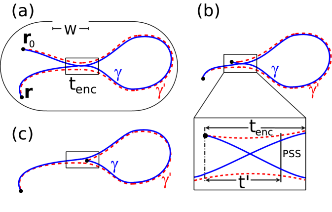
For their evaluation consider the time $t^{\prime}$ between the initial or final point of the trajectory and the PSS, defined in the zoom into Fig. 1(b). Then $t_{\rm enc}(t^{\prime},u)\!=\!=t^{\prime}\!+\!\lambda^{-1}\!\ln(c/|u|)$ and $S_{\gamma}\!-\!S_{\gamma^{\prime}}\!=\!su$ for any position of the PSS. The density of encounters is $w_{\rm 1ll}(s,u,t)\!=\!2\int_{0}^{\lambda^{-1}\ln(c/|s|)}dt^{\prime}\![t\!-\!2t_{\rm enc}(t^{\prime},u)]/[\Omega(E)t_{\rm enc}(t^{\prime},u)]$, where the prefactor 2 accounts for the two cases of beginning or ending in an encounter region. We evaluate this contribution by modifying $\rho_{\rm cl}(t)$ by $e^{t_{\rm enc}/\tau_{d}}$ as before and integrating over $s$, $u$ and $t^{\prime}$. To this end we substitute ref:Brouwer06 $t^{\prime\prime}\!=\!t^{\prime}+\lambda^{-1}\ln(c/|u|)$, $\sigma\!=\!c/u$ and $x\!=\!su/c^{2}$, with integration domains $-1\!<\!x\!<\!1$, $1\!<\!\sigma\!<\!e^{\lambda t^{\prime\prime}}$ and $0\!<\!t^{\prime\prime}\!<\!\lambda^{-1}\!\ln(1/|x|)$. Note that the limits for $t^{\prime}$ include the case when the paths do not have a self-crossing in configuration space (Fig. 1(c)). The integration yields

It precisely cancels the linear term in $\rho_{\rm 2ll}$, Eq. (4), i.e. $\rho_{\rm 2ll}(t)\!+\!\rho_{\rm 1ll}(t)\!=\!e^{-t/\tau_{d}}t^{2}/(2\tau_{d}t_{H})$, recovering unitarity!

The next-order quantum corrections are obtained by calculating ref:Gutierrez 1ll and 2ll contributions of diagrams such as discussed in ref:Heusler . Together with Eqs. (4,5), this yields for systems with time reversal symmetry

for $t<t^{*}$. The term quadratic in $t$ represents the weak localization-type enhancement of the quantum survival probability. The quadratic and the quartic terms, which agree with RMT ref:Frahm97 , dominate for the time range considered. The cubic term in Eq. (6), whose functional form was anticipated in ref:Frahm97 , scales differently with $\tau_{d}$ and $t_{H}$.

For systems without time reversal symmetry the calculation of the relevant one- and two-leg-loops gives, again in accordance with RMT ref:Frahm97 ,

We finally note that our restriction to localized initial states can be lifted and the results generalized to arbitrary initial states ref:Gutierrez . This is because the trajectory pairs $\bar{\gamma},\bar{\gamma}^{\prime}$ survive the integration in Eq. (3) only if their starting points are close to each other in phase space, rendering the above analysis valid.

Continuity equation.– It is instructive to reformulate the decay problem in terms of paths crossing the opening. To this end we consider the integral version of the continuity equation, $\partial\rho({\mathbf{r}},t)/\partial t\!+\!\nabla\!\cdot\!\mathbf{j}(\mathbf{r},t)\!=\!0$, namely

where $S$ is the cross section of the opening with a normal vector $\hat{n}_{x}$. In Eq. (8), the current density $\mathbf{j}(\mathbf{r},t)\!=\!(1/m){\rm Re}[(\hbar/i)\psi^{*}(\mathbf{r},t)\mathbf{\nabla}\psi(\mathbf{r},t)]$ can be semiclassically expressed through Eq. (2) in terms of orbit pairs connecting points inside $A$ with the opening. In the diagonal approximation we obtain $\int_{S}\mathbf{j}_{\rm diag}\cdot\hat{n}_{x}dx=e^{-t/\tau_{d}}/\tau_{d}$, consistent with $\rho_{\rm cl}(t)$. Loop contributions are calculated analogously to those of $\rho_{\rm sc}$ from Eq. (3), giving

Time integration of Eq. (8) leads to $\rho_{\rm 2ll}(t)\!+\!\rho_{\rm 1ll}(t)\!=\!e^{-t/\tau_{d}}t^{2}/(2\tau_{d}t_{H})$, consistent with Eq. (6). The 1ll contributions enter into Eq. (9) with half the weight, since 1lls with a short leg (encounter box) at the opening must be excluded. These ’missing’ paths assure the correct form of quantum deviations from $\rho_{\rm cl}(t)$.

Higher 2ll and 1ll corrections to $\mathbf{j}$ lead to Eqs. (6,7). We conclude that both, 2ll and 1ll contributions to $\mathbf{j}$ are essential to achieve a unitary flow and thereby to establish a semiclassical version of the continuity equation.

Ehrenfest time effects.– The Ehrenfest time $\tau_{E}$ ref:Chirikov separates the evolution of wave packets following essentially the classical dynamics from longer time scales dominated by wave interference. While $\tau_{E}$-effects have been mainly considered for stationary processes involving time integration ref:Aleiner96 ; ref:Yevtushenko00 ; ref:Adagideli03 ; ref:Ehrenfest2 ; ref:Brouwer06 ; ref:Jacquod06 , signatures of $\tau_{E}$ should appear most directly in the time domain ref:Brouwer06B ; ref:Schomerus04 , i.e. for $\rho(t)$. Here we semiclassically compute the $\tau_{E}$-dependence of the weak-localization correction to $\rho(t)$ in Eq. (6). To this end we distinguish between $\tau_{E}^{\rm c}\!=\!\lambda^{-1}\!\ln({\mathcal{L}}/\lambda_{B})$, where ${\mathcal{L}}$ is the typical system size and $\lambda_{B}$ the de Broglie wavelength, and $\tau_{E}^{\rm o}\!=\!\lambda^{-1}\!\ln(w^{2}/({\mathcal{L}}\lambda_{B}))$, related to the width $w$ of the opening ref:Jacquod06 . As before we consider that the densities $w_{\rm 2ll,1ll}(s,u,t)$ contain the Heaviside function $\theta(t\!-\!2t_{\rm enc})$ (negligible for $\tau_{E}^{\rm o,c}\ll\tau_{d}$) assuring that the time required to form a 1ll or 2ll is larger than $2t_{\rm enc}$. Our calculation gives (for $\tau_{E}^{\rm o,c}\lambda\gg 1$ with $2\tau_{E}^{\rm e}\!=\!\tau_{E}^{\rm o}+\tau_{E}^{\rm c}$)

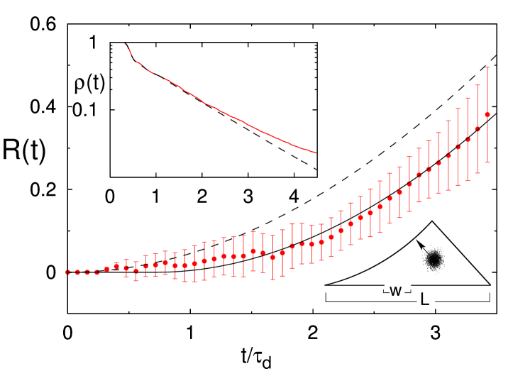
Numerical simulation.– The leading-order quantum corrections in Eq. (6) and (7) were confirmed by numerical simulations for graphs ref:Puhlmann05 . Here we compare our semiclassical predictions with quantum calculations of $\rho(t)$ based on the numerical propagation of Gaussian wave packets inside a billiard, a setup much closer to experiment. We chose the desymmetrized diamond billiard (inset Fig. 2) ref:Goussev07 that is classically chaotic ($\lambda^{-1}\simeq 3\tau_{f}$, with $\tau_{f}$ the mean free flight time). Its opening $w$ corresponds to $N\!=\!10$ open channels and to $\tau_{d}\!\simeq\!15\tau_{f}$. For the simulations, we reach $t_{H}\!=\!10.6\tau_{d}$ implying $t^{\ast}\!=\!3.3\tau_{d}$, $\tau_{E}^{\rm o}\!\simeq\!0.17\tau_{d}$ and $\tau_{E}^{\rm c}\!\simeq\!0.55\tau_{d}$ (with $\mathcal{L}\!=\!\sqrt{A}$).

In the upper inset of Fig. 2 we compare the decay, $\rho^{\rm sim}_{\rm qm}(t)$ (red full line), for a representative wave packet simulation with the corresponding classical, $\rho^{\rm sim}_{\rm cl}(t)$ (dashed line), obtained from an ensemble of trajectories with the same phase space distribution as the Wigner function of the initial quantum state. $\rho^{\rm sim}_{\rm cl}(t)$ merges into the exponential decay $\exp(-t/\tau_{d})$, and $\rho^{\rm sim}_{\rm qm}(t)$ coincides with $\rho^{\rm sim}_{\rm cl}(t)$ up to scales of $t^{\ast}$. For a detailed analysis of the quantum deviations we consider the ratio $R(t)\!\equiv\![\rho^{\rm sim}_{\rm qm}(t)\!-\!\rho^{\rm sim}_{\rm cl}(t)]/\rho^{\rm sim}_{\rm cl}(t)$. The red symbols in Fig. 2 represent an average of $R(t)$ over 27 different opening positions and initial momentum directions. The dashed and full curve depict the semiclassical results based on the quadratic term in Eq. (6) (dominant for the $t/\tau_{d}$-range displayed) and on Eq. (10). The overall agreement of the numerical data with the full curve indicates $\tau_{E}$-signatures. We note, however, that we cannot rule out other non-universal effects (e.g. due to scars ref:Kaplan , short orbits, diffraction or fluctuations of the effective $\tau_{d}$ ref:Casati ) that may also yield time shifts. Furthermore the individual numerical traces $R(t)$ exhibit strong fluctuations (reflected in a large variance in Fig. 2). A numerical confirmation of the $\log(1/\hbar)$-dependence of $\tau_{E}$ seems to date impossible for billiards.

Photo-ionization and -dissociation cross sections.– Related to the decay problem are photo absorption processes where a molecule ref:Schinke93 (or correspondingly an atom) is excited into a classically chaotic, subsequently decaying resonant state. In dipole approximation, the photo-dissociation cross section of the molecule excited from the ground state $|g\rangle$ is $\sigma(\epsilon)\!=\!{\rm Im}{\rm Tr}\{\hat{A}G(\epsilon)\}$, where $G(\epsilon)$ is the retarded molecule Green function, $\hat{A}\!=\![\epsilon/(c\hbar\epsilon_{0})]|\phi\rangle\langle\phi|$ and $|\phi\rangle\!=\!D|g\rangle$, with $D\!=\!{\bf d}\!\cdot\!\hat{{\bf e}}$ the projection of the dipole moment on the light polarization $\hat{\bf e}$. The two-point correlation function of $\sigma(\epsilon)$ is defined as

where $\langle{\sigma}(\epsilon)\rangle_{\epsilon}\approx\pi(2\pi\hbar)^{-2}\!\int{\mathbf{d}r}{\mathbf{d}p}A_{W}({\mathbf{r}},{\mathbf{p}})\delta(\epsilon\!-\!H({\mathbf{r}},{\mathbf{p}}))$ semiclassically, with Wigner transform $A_{W}$ of $\hat{A}$. Previous semiclassical treatments of $C(\omega)$ ref:Agam00 ; ref:Eck00 were limited to the diagonal approximation. To compute off-diagonal (loop) terms we consider $Z(\tau)\!=\!\int_{-\infty}^{\infty}d\omega e^{2\pi i\omega\tau}C(\omega)$ with $\tau\!=\!t/t_{H}$. Semiclassically, $Z_{\rm sc}$ is again given by a double sum over orbits with different initial and final points. Due to rapidly oscillating phases from the action differences, only two possible configurations of those points contribute ref:Agam00 : (i) orbits in a sum similar to Eq. (3) leading to a contribution as for $\rho_{\rm sc}(t)$; (ii) trajectories in the vicinity of a periodic orbit. Expanding around it, as in ref:Eck00 , leads to the spectral form factor $K^{\rm open}_{\rm sc}(\tau)$ of an open system. From (i) and (ii) we have $Z_{\rm sc}(\tau)\!=\!K^{\rm open}_{\rm sc}(\tau)\!+\!2\rho_{\rm sc}(\tau)$ for the time reversal case. Up to second order in $\tau\!>\!0$ we find $K^{\rm open}_{\rm sc}(\tau)\!=\!{\rm e}^{-N\tau}(2\tau-2\tau^{2})$ and $\rho_{\rm sc}(\tau)\!=\!{\rm e}^{-N\tau}(1+N\tau^{2}/2)$ (Eq. (6)), Thereby $Z_{\rm sc}(\tau)\!=\!e^{-N\tau}[2\!+\!2\tau\!+\!(N\!-\!2)\tau^{2}]$, confirming a conjecture of ref:Gorin05 . Its inverse Fourier transform yields the two-point correlation (with $\Gamma=2\pi\omega\tau_{d}/t_{H}$)

The first two diagonal terms agree with ref:Agam00 ; the third term represents the leading quantum correction.

To conclude, we presented a general semiclassical approach to the problems of quantum decay and photo cross-section statistics in open chaotic quantum systems.

We thank I. Adagideli, J. Kuipers and C. Petitjean for useful discussions and for a critical reading of the manuscript. We acknowledge funding by DFG under GRK 638 and the A. von Humboldt Foundation (AG).

References

- (1) for a recent account of quantum chaotic scattering see e.g., J. Phys. A 38, Special Issue no. 49 (2005).
- (2) V. Milner et al., Phys. Rev. Lett. 86, 1514 (2001).
- (3) N. Friedman et al., Phys. Rev. Lett. 86, 1518 (2001).
- (4) C. M. Marcus et al., Phys. Rev. Lett. 69, 506 (1992).
- (5) E. Doron, U. Smilansky, and A. Frenkel, Phys. Rev. Lett. 65, 3072 (1990).
- (6) G. Stania and H. Walther, Phys. Rev. Lett. 95, 194101 (2005).
- (7) G. Casati, G. Maspero, and D. Shepelyansky, Phys. Rev. E 56, R6233 (1997).
- (8) K. Frahm, Phys. Rev. E 56, R6237 (1997).
- (9) D. Savin and V. Sokolov, Phys. Rev. E 56, R4911 (1997).
- (10) for a comprehensive analysis of (scar) effects beyond RMT, see L. Kaplan, Phys. Rev. E 59, 5325 (1999).
- (11) M. Puhlmann et al., Europhys. Lett. 69, 313 (2005).
- (12) M. Sieber and K. Richter, Phys. Scr. T90, 128 (2001); M. Sieber, J. Phys. A 35, 613 (2002).
- (13) S. Müller et al., Phys. Rev. Lett. 93, 014103 (2004).
- (14) P. W. Brouwer, S. Rahav, and C. Tian, Phys. Rev. E 74, 066208 (2006).
- (15) K. Richter and M. Sieber, Phys. Rev. Lett. 89, 206801 (2002).
- (16) I. Adagideli, Phys. Rev. B 68, 233308 (2003).
- (17) S. Rahav and P. W. Brouwer, Phys. Rev. Lett. 96, 196804 (2006).
- (18) P. W. Brouwer and S. Rahav, Phys. Rev. B 74, 075322 (2006).
- (19) Ph. Jacquod and R. S. Whitney, Phys. Rev. B 73, 195115 (2006).
- (20) S. Heusler et al., Phys. Rev. Lett. 96, 066804 (2006).
- (21) J. Kuipers and M. Sieber, Phys. Rev. E, in press (2008).
- (22) M. Gutzwiller, Chaos in Classical and Quantum Mechanics, (Springer, New York, 1990).
- (23) We consider times for a chaotic system with Lyapunov exponent and a small opening such that , while the number of channels is still large.
- (24) Orbits where and are inside the encounter region, i.e. responsible for coherent backscattering, yield negligible contributions in the semiclassical limit ref:Gutierrez .
- (25) M. Gutiérrez et al., in preparation.
- (26) B. V. Chirikov, F M. Izrailev, and D. L. Shepelyanskii, Sov. Sci. Rev. C 2, 209 (1981).
- (27) I. L. Aleiner and A. I. Larkin, Phys. Rev. B 54, 14423 (1996).
- (28) O. Yevtushenko et al., Phys. Rev. Lett. 84, 542 (2000).
- (29) H. Schomerus and J. Tworzydlo, Phys. Rev. Lett. 93, 154102 (2004); H. Schomerus and Ph. Jacquod, J. Phys. A 38, 10663 (2005).
- (30) For more details of the simulations see A. Goussev and K. Richter, Phys. Rev. E 75 015201 (2007).
- (31) R. Schinke, Photodissociation Dynamics (Cambridge University Press, Cambridge, 1993).
- (32) O. Agam, Phys. Rev. E 61, 1285 (2000).
- (33) B. Eckhardt, S. Fishman, and I. Varga, Phys. Rev. E 62, 7867 (2000).
- (34) T. Gorin, J. Phys. A 38, 10805 (2005).