Semiparametric Inference of the Complier Average Causal Effect with Nonignorable Missing Outcomes
Abstract
Noncompliance and missing data often occur in randomized trials, which complicate the inference of causal effects. When both noncompliance and missing data are present, previous papers proposed moment and maximum likelihood estimators for binary and normally distributed continuous outcomes under the latent ignorable missing data mechanism. However, the latent ignorable missing data mechanism may be violated in practice, because the missing data mechanism may depend directly on the missing outcome itself. Under noncompliance and an outcome-dependent nonignorable missing data mechanism, previous studies showed the identifiability of complier average causal effect for discrete outcomes. In this paper, we study the semiparametric identifiability and estimation of complier average causal effect in randomized clinical trials with both all-or-none noncompliance and the outcome-dependent nonignorable missing continuous outcomes, and propose a two-step maximum likelihood estimator in order to eliminate the infinite dimensional nuisance parameter. Our method does not need to specify a parametric form for the missing data mechanism. We also evaluate the finite sample property of our method via extensive simulation studies and sensitivity analysis, with an application to a double-blinded psychiatric clinical trial.
Key Words: Causal inference; Instrumental variable; Missing not at random; Noncompliance; Outcome-dependent missing; Principal stratification.
1 Introduction
Randomization is an effective way to study the average causal effects (s) of new drugs or training programs. However, randomized trials are often plagued with noncompliance and missing data, which may make statistical inference difficult and biased. The noncompliance problem happens when some subjects fail to comply with their assigned treatments, and the missing data problem happens when investigators fail to collect information for some subjects. Ignoring noncompliance and missing data problems may lead to biased estimators of the s.
The noncompliance problem has attracted a lot of attention in the literature. Efron and Feldman (1991) studied the noncompliance problem before the principal stratification framework (Frangakis and Rubin, 2002) was proposed. In the presence of noncompliance, Balke and Pearl (1997) proposed large sample bounds of the s for binary outcomes using the linear programming method. Angrist et al. (1996) discussed the identifiability of the causal effect using the instrumental variable method. Imbens and Rubin (1997) proposed a Bayesian method to estimate the complier average causal effect (). When some outcomes are missing, the identifiability and estimation of are more complicated, and different types of missing data mechanisms have sizable impacts on the identifiability and estimation of . Frangakis and Rubin (1999) established the identifiability and proposed a moment estimator of under the latent ignorable (LI) missing data mechanism. Under the LI missing data mechanism, Zhou and Li (2006) and O'Malley and Normand (2005) proposed Expectation-Maximization (EM) algorithms (Dempster et al., 1977) to find the maximum likelihood estimators (MLEs) of for binary and normally distributed outcomes, respectively. Barnard et al. (2003) proposed a Bayesian approach to estimate with bivariate outcomes and covariate adjustment. Taylor and Zhou (2011) proposed a multiple imputation method to estimate for clustered encouragement design studies.
However, the LI assumption may be implausible in some clinical studies when the missing data mechanism may depend on the missing outcome. Chen et al. (2009) and Imai (2009) discussed the identifiability of for discrete outcomes under the outcome-dependent nonignorable (ODN) missing data mechanism. To the best of our knowledge, there are no published papers in the literature studying the identifiability of for continuous outcomes under the ODN assumption. In this paper, we show that is semiparametrically identifiable under some regular conditions, and propose estimation methods for with continuous outcomes under the ODN assumption. For our semiparametric method, we need only assume that the distribution of the outcomes belongs to the exponential family without specifying a parametric form for the missing data mechanism.
This paper proceeds as follows. In Section 2, we discuss the notation and assumptions used in this paper and define the parameter of interest. In Section 3, we show the semiparametric identifiability and propose a two-step maximum likelihood estimator (TSMLE). In Section 4, we use several simulation studies to illustrate the finite sample properties of our proposed estimators and consider sensitivity analysis to assess the robustness of our estimation strategy. In Section 5, we analyze a double-blinded randomized clinical trial using the methods proposed in this paper. We conclude with a discussion and provide all proofs in the Appendices.
2 Notation and Assumptions
We consider a randomized trial with a continuous outcome. For the -th subject, let denote the randomized treatment assignment ( for treatment and for control). Let denote the treatment received ( for treatment and for control). When , there exists noncompliance. Let denote the outcome variable. Let denote the missing data indicator of , i.e., if is observed and if is missing. First, we need to make the following fundamental assumption.
- Assumption 1 (Stable unit treatment value assumption, SUTVA):
Except in the dependent case for infectious diseases (Hudgens and Halloran, 2008), the SUTVA assumption is reasonable in many cases. Under the SUTVA assumption, we define and as the potential treatment received, the potential outcome measured, and the potential missing data indicator for subject if he/she were assigned to treatment . These variables are potential outcomes because only one of the pairs and can be observed. Since is the observed treatment assignment for subject , , and are the observed treatment received, the observed outcome, and the observed missing data indicator.
Under the principal stratification framework (Angrist et al., 1996; Frangakis and Rubin, 2002), we let be the compliance status of subject , defined as follows:
| (5) |
where and represent ``always-taker'', ``complier'', ``defier'' and ``never-taker'', respectively. Here is an unobserved variable, because we can observe only or for subject , but not both. The of to is the parameter of interest, defined as
is a subgroup causal effect for the compliers, with incompletely observed compliance status. Next, we give some sufficient conditions about the latent variables to make identifiable, in the presence of noncompliance and nonignorable missing outcomes.
- Assumption 2 (Randomization):
-
The treatment assignment is completely randomized.
Randomization means that is independent of , and we define . Under the randomization assumption, can be expressed as
- Assumption 3 (Monotonicity):
-
for each subject .
The monotonicity of implies that there are no defiers. Define for , and the monotonicity assumption implies . Assumption 3 is plausible when the treatment assignment has a nonnegative effect on the treatment received for each subject, and it holds directly when the treatment is not available to subjects in the control arm, meaning for all subjects. The monotonicity assumption implies a positive of on . However, under general circumstances, Assumption 3 is not fully testable, since only one of and can be observed.
- Assumption 4:
-
By randomization, we have that under Assumption 4, and therefore is correlated with . Without Assumption 4, we have , which implies that under Assumption 3. Since we are interested in the identifiability of , Assumption 4 is necessary.
- Assumption 5 (Compound exclusion restrictions):
-
For never-takers and always-takers, we assume , and .
The traditional exclusion restriction assumes for and . Frangakis and Rubin (1999) extended it to the compound exclusion restrictions, and imposed similar assumption on the joint vector of the outcome and the missing data indicator. Assumption 5 is reasonable in a double-blinded clinical trial, because the patients do not know the treatment assigned to them and thus has no ``direct effect'' on the outcome and the missing data indicator. However, when the missing data indicator depends on the treatment assigned, the compound exclusion restrictions may be violated. When is randomized, Assumption 5 is equivalent to and
- Assumption 6 (Outcome-dependent nonignorable missing data):
-
For all ; and , we assume
(6) (7)
When is randomized, the equation (6) becomes and (7) becomes . Define . Therefore Assumption 2 and Assumption 6 imply that . Hence depends on , but is independent of given .
In previous papers (Frangakis and Rubin, 1999; O'Malley and Normand, 2005; Zhou and Li, 2006), the LI assumption is used for modeling missing data, which means that the potential outcomes and associated potential nonresponse indicators are independent within each principal stratum, that is . Under the ODN missing data mechanism, the missing data indicator depends on the possibly missing outcome , which may be more reasonable than the LI missing data assumption in some applications. For example, some patients may have higher probabilities to leave the trial if their health outcomes are not good, and they may be more likely to stay in the trial otherwise. We illustrate the LI and ODN missing data mechanisms using the graphical models in Figure 1. Note that the arrows from to are absent because of the compound exclusion restriction assumption.
| (a) LI under Assumptions 2 and 5 | (b) ODN under Assumptions 2 and 5 |
3 Semiparametric Identifiability and Estimation
In this section, we first discuss the difficulty of nonparametric identifiability without assuming a parametric form for both the outcome distribution and the missing data mechanism. If both the distribution of the outcome and the missing data mechanism are not specified, the model is essentially not identifiable without further assumptions. We then propose a semiparametric method, specifying only the distribution of without assuming any parametric form for the missing data mechanism. We show the identifiability and propose a TSMLE of under the assumption that the distribution of the outcome variable belongs to the exponential family.
3.1 Semiparametric Identifiability
Under SUTVA, randomization and monotonicity assumptions, we have , , , and . These parameters can be identified directly from the observed data. Next we focus on the identification of the parameters of .
- Assumption 7:
-
The conditional density of the outcome variable belongs to the following exponential family:
(8) where , and are known functions, and are unknown parameters. We denote simply as hereinafter.
The parametric assumption of the outcome is untestable in general, since the missing data mechanism depends arbitrarily on the outcome. But for binary outcome, Small and Cheng (2009) proposed a goodness-of-fit test for the model under the ODN missing data mechanism. When the randomization assumption holds, the is the difference between the expectations of the conditional density of , that is
Hence if the parameters of are identified, the is also identified. The exponential family defined by Assumption 7 includes many common distributions, such as normal distributions , exponential distributions with mean parameter , Gamma distributions with shape parameter and rate parameter , and the log-normal distributions , where s are specified as , , , and , respectively.
Next, Theorem 1 will show the identifiability of the parameters of . The proof of Theorem 1 is provided in Appendix A. Assumption 5 implies and , which can be simplified as and respectively.
Theorem 1.
Under Assumptions 1 to 7, the vector , , , , , , , , , is identifiable. If there exists a one-to-one mapping from the parameter set to the vector , then is identifiable and so is
The one-to-one mapping condition seems complicated, but it is reasonable and holds for many widely-used distributions, such as homoskedastic normal distributions, exponential distributions, etc. We will verify the one-to-one mapping condition for normal and exponential distributions in Appendix C and Appendix D. Other distributions such as heteroskedastic normal distributions, Gamma distributions and lognormal distributions can be verified similarly. However, counterexamples do exist, and we provide one in Appendix A.
3.2 TSMLE of
Because we do not specify a parametric form on the missing data mechanism , the joint distribution of is not specified completely. Thus the MLEs of parameters are hard to obtain, since the likelihood depends on the infinite dimensional parameter as shown in Appendix B. In this subsection, we propose a two-step likelihood method to estimate parameters, which can be viewed as an example of the Two-Step Maximum Likelihood studied by Murphy and Topel (2002).
In the first step, a consistent estimator for can be obtained by MLE using the data . Let denote the sample size, , and for and . Then the log likelihood function for is
| (9) |
The MLE for is , equivalent to the moment estimator.
In the second step, we propose a conditional likelihood method to estimate the parameter set , which is based on the conditional probability of given and . Here the proposed conditional likelihood function does not depend on the nuisance parameter , based on the fact that the following equations (3.2) to (12) do not depend on :
| (12) |
It is obvious that
| (13) |
The left hand sides of equations (3.2) to (12) consist of and , with the latter identified from the first step. The right hand sides of equations (3.2) to (12) consist of the parameters of interest. Therefore we can estimate through a likelihood method. Note the right hand sides do not depend on , so we do not need to specify the form of . Let denote . Since given follows a multinomial distribution with four categories, the conditional log-likelihood function of can be written as
| (14) |
From the proof of Theorem 1, the parameter can be identified from the second likelihood function (14) after identifying from the first likelihood function (9). Therefore, by maximizing over , we obtain the maximizer . In practice, we can use the bootstrap method to approximate the sampling variance of the estimator of
4 Simulation Studies and Sensitivity Analysis
We report simulation studies and sensitivity analyses in order to evaluate the finite sample properties of the estimating methods proposed in this paper. In Tables 2-4, the columns with labels ``bias'', `` '', `` CP'' and `` CI'' represent the average bias, standard deviation, coverage proportion and average confidence interval, respectively.
First, we generate the outcomes under the ODN missing data mechanism from homoskedastic normal distributions (denoted as ``''), exponential distributions, Gamma distributions and log-normal distributions, respectively. We set the number of simulations to be , and choose the sample sizes as , and , respectively. We show the joint distributions of in Table 1, and report the results in Table 2. The results have small biases and standard deviations, which decrease as the sample sizes become larger. And all the confidence intervals of have empirical coverage proportions very close to their nominal values.
| Exponential | Gamma | Lognormal | ||
| Bernoulli(0.5) | ||||
| true value | bias | CP | CI | ||
|---|---|---|---|---|---|
| 500 | -0.0194 | 0.3395 | 0.9489 | [0.3152, 1.6461] | |
| 1000 | -0.0073 | 0.2343 | 0.9476 | [0.5335, 1.4518] | |
| 2000 | 0.0022 | 0.1629 | 0.9500 | [0.6828, 1.3215] | |
| 4000 | -0.0019 | 0.1145 | 0.9504 | [0.7736, 1.2225] | |
| 500 | 0.0872 | 1.5910 | 0.9455 | [-2.0312, 4.2056] | |
| 1000 | 0.0312 | 1.0309 | 0.9441 | [-0.9893, 3.0517] | |
| 2000 | 0.0106 | 0.7091 | 0.9479 | [-0.3793, 2.4004] | |
| 4000 | 0.0072 | 0.4891 | 0.9506 | [0.0486, 1.9657] | |
| 500 | 0.0830 | 1.6872 | 0.9915 | [-2.2237, 4.3901] | |
| 1000 | 0.0284 | 0.5978 | 0.9625 | [-0.1432, 2.2000] | |
| 2000 | 0.0108 | 0.3636 | 0.9493 | [0.2981, 1.7235] | |
| 4000 | 0.0032 | 0.2530 | 0.9505 | [0.5073, 1.4992] | |
| 500 | 0.1156 | 0.7849 | 0.9617 | [-0.3806, 2.6962] | |
| 1000 | 0.0599 | 0.4571 | 0.9494 | [0.2061, 1.9981] | |
| 2000 | 0.0218 | 0.3093 | 0.9496 | [0.4578, 1.6702] | |
| 4000 | 0.0106 | 0.2130 | 0.9469 | [0.6353, 1.4702] |
Second, we report the results of comparison of our methods with the MLE proposed by O'Malley and Normand (2005) (``LI'' in Tables 3) under five different cases, which violate the homoskedastic normal outcomes or the ODN assumption. We repeat our simulation times with sample sizes of in each case. The results of five cases are shown in Table 3, named as ``Heter'', ``Unif'',``T'', ``DY'' and ``DYU'', respectively. The first case, ``Heter'' case, violates the homoskedastic normal outcomes. Next two cases, ``Unif'' and ``T'', violate the exponential family assumption. The last two cases, ``DY'' and ``DYU'', violate the ODN assumption. In the ``Heter'' case we generate data from heteroskadastic normal outcomes. The data generating process is the same as ``'' except that , for . In the `Unif'' case the data is generated the same as ``'' except that the outcomes follow uniform distribution with , , and , respectively. The data generating process in the ``T'' case is the same as ``'' except that the outcomes follow t distributions with the same means as ``'' and degrees of freedom . In the ``DY'' case we generate data under the missing data mechanism depending on both and , and choose with other conditional distributions the same as ``''. In the ``DYU'' case we generate data with the missing data mechanism depending on , and , and choose , with other conditional distributions the same as ``'' and corresponding to . From Table 3, we can see that the point estimator of our method is generally robust to four kinds of violations of the assumptions. However, the results are worse for ``Unif'' case, which has a large bias, low coverage proportion and whose confidence interval does not cover the true value.
| Method | Assump. | bias | CP | CI | |
|---|---|---|---|---|---|
| ODN | Heter | -0.0268 | 0.0772 | 0.9363 | [0.8220, 1.1244] |
| Unif | -0.3815 | 0.1865 | 0.4676 | [0.2530, 0.9841] | |
| T | -0.0350 | 0.1730 | 0.9427 | [0.6960, 1.3740] | |
| DY | 0.0201 | 0.1555 | 0.9465 | [0.7154, 1.3249] | |
| DYU | -0.0852 | 0.1691 | 0.9242 | [0.5834, 1.2462] | |
| LI | Heter | -0.0277 | 0.0677 | 0.9300 | [0.8395, 1.1051] |
| Unif | -0.8521 | 0.2474 | 0.0695 | [-0.3369, 0.6327] | |
| T | 0.2244 | 0.1225 | 0.5577 | [0.9843, 1.4646] | |
| DY | -0.0288 | 0.0894 | 0.9370 | [0.7959, 1.1465] | |
| DYU | -0.1267 | 0.1321 | 0.8426 | [0.6144, 1.1322] |
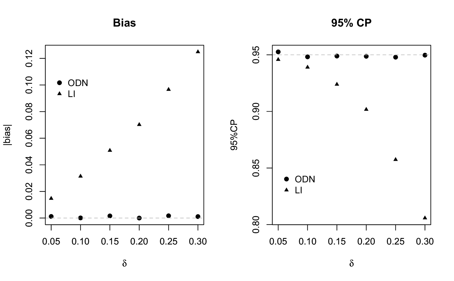
Finally, we compare our methods with the MLE proposed by O'Malley and Normand (2005) under the LI missing data mechanism (``LI'' in Table 4). We repeat our simulation times with sample sizes of in each case. The data generating processes are the same as ``'', but the missing data mechanisms are LI. Denote , and choose , , and for ``LI1'' to ``LI4'' respectively as shown in rows 1-4 and 5-8 of Table 4. Since the missing data mechanisms are LI, the ``LI'' method exhibits very small biases. Although the assumptions required by the ``ODN'' methods do not hold, the biases are not very large except for the missing mechanism LI4. The last case, LI4, has the largest variability among the 's and thus the largest bias for estimating the , since the missing data mechanism has the ``strongest'' dependence on and but not . Next we generate data under the ODN assumption, and compare the methods under both ODN and LI assumptions. Let where . As increases, the relationship between and becomes stronger. The data are generated from the same joint distribution as ``'' except for different . The results are shown in Figure 2. The method under ODN missing data mechanism has small bias and promising coverage property irrespective of , but the method under LI missing data mechanism has larger bias and poorer coverage property with larger .
| Method | bias | CP | CI | ||
|---|---|---|---|---|---|
| ODN | LI1 | -0.0291 | 0.1236 | 0.9438 | [0.7287, 1.2132] |
| LI2 | 0.0976 | 0.1452 | 0.8961 | [0.8130, 1.3823] | |
| LI3 | -0.0569 | 0.1371 | 0.9332 | [0.6745, 1.2118] | |
| LI4 | -0.1961 | 0.1152 | 0.5966 | [0.5781, 1.0297] | |
| LI | LI1 | -0.0013 | 0.1123 | 0.9491 | [0.7785, 1.2189] |
| LI2 | -0.0010 | 0.1099 | 0.9504 | [0.7836, 1.2145] | |
| LI3 | -0.0008 | 0.1262 | 0.9502 | [0.7519, 1.2465] | |
| LI4 | -0.0015 | 0.1290 | 0.9505 | [0.7456, 1.2515] |
5 Application
We use the new methods proposed in this paper to re-analyze a psychiatric clinical trial. It is a double-blinded randomized study comparing the relative effect of clozapine and haloperidol in adults with refractory schizophrenia at fifteen Veterans Affairs medical centers. Clozapine is found to be more efficacious than standard drugs in patients with refractory schizophrenia. Yet it is associated with potentially fatal agranulocytosis. One objective for conducting this trial is to evaluate the clinical effect of two antipsychotic medications. The dataset has been analysed in Rosenheck et al. (1997), Levy et al. (2004), and O'Malley and Normand (2005). Some summary statistics of the data are described in Table 5. More details about the trial can be found in Rosenheck et al. (1997) and O'Malley and Normand (2005). In the treatment arm, patients are randomized to clozapine; in the control arm, patients are randomized to haloperidol. The outcome of interest is the positive and negative syndrome score (PANSS) with higher values indicating more severe symptoms. The baseline PANSS is nearly balanced in both groups. Missing outcome patterns are obviously different in the clozapine group (about ) than in the haloperidol group (about ). Hence it is possible that outcomes are not missing at random. The primary reasons for dropout in the clozapine group are side effects or non-drug-related reasons. The reasons for discontinuing haloperidol are lack of efficacy or worsening of symptoms. Therefore, the missing mechanism may possibly depend on the missing outcome, and we think that the ODN assumption may be more reasonable in this case.
| Received treatment | |||
| Assigned treatment | Clozapine () | Haloperidol () | Total |
| Clozapine () | |||
| Sample size | 122 | 81 | 203 |
| Missing sample size | 0 | 40 | 40 |
| Mean of the baseline PANSS | 90.83 | 91.20 | 90.98 |
| Haloperidol () | |||
| Sample size | 57 | 161 | 218 |
| Missing sample size | 12 | 47 | 59 |
| Mean of the Baseline PANSS | 96.30 | 90.69 | 92.16 |
The estimates of by different methods are shown in Table 6. In Table 6, the ``homo'' and ``hetero'' in parentheses after ``ODN'' correspond to the homoskedastic and heteroskedastic model assumptions, respectively; and ``LI'' corresponds to the MLE proposed in O'Malley and Normand (2005). The columns of Table 6 correspond to the methods, point estimates, standard errors, and confidence intervals, respectively. The bootstrap method is used to compute standard errors and confidence intervals for all methods. From Table 6, we can see that under the homoskedastic assumption subjects in the clozapine group had lower symptom levels than those in the haloperidol group, and under the heteroskedastic assumption it was . Both methods have similar conclusions that clozapine is somewhat more effective than haloperidol for patients with refractory schizophrenia. Both of the semiparametric methods give insignificant results since both confidence intervals include zero. Our results are similar to O'Malley and Normand (2005) which also gave an insignificant result. However, the results of the confidence intervals are somewhat different: the result under the ODN mechanism with the heteroskedastic assumption is significant, but the results from other two models are not.
Assuming different missing data mechanisms such as LI, ODN and under other different assumptions on the outcome variable, we can find different point estimates and confidence intervals for using the data from the psychiatric clinical trial. When we have prior knowledge that the missing mechanism depends only on the treatment received and the compliance status, the method under LI missing mechanism will provide more credible conclusion. However, when we have prior knowledge that the missing mechanism depends directly on the outcome, we recommend our methods under the ODN missing data mechanism. The newly proposed methods can be used as alternatives for the predominate methods assuming the LI missing mechanism in sensitivity analysis.
| Method | Estimate | CI | CI | |
|---|---|---|---|---|
| ODN(homo) | -5.00 | 3.05 | [-10.98, 0.98] | [-10.02, 0.02] |
| ODN(hetero) | -5.54 | 3.05 | [-11.52, 0.44] | [-10.56, -0.52] |
| LI | -4.36 | 4.35 | [-12.89, 4.17] | [-11.52, 2.80] |
6 Discussion
Randomization is a powerful tool to measure the relative causal effect of treatment versus control. Some subjects in randomized trials, however, may fail to comply with the assigned treatments or drop out before the final outcomes are measured. Noncompliance and missing data problems make statistical causal inference difficult, because the causal effects are not identifiable without additional assumptions. Under different assumptions about the missing data mechanisms of the outcomes, the identifiability and estimation methods may be fundamentally different. Most previous studies (Frangakis and Rubin, 1999; Barnard et al., 2003; O'Malley and Normand, 2005; Zhou and Li, 2006) rely on the LI assumption in order to identify , but the LI assumption may be not reasonable when the missing data mechanism may depend on the outcome. Under the ODN missing data mechanism, Chen et al. (2009) and Imai (2009) showed the identifiability and proposed the moment estimator and the MLE of for discrete outcomes. But there are no results for continuous outcomes under both noncompliance and ODN missing data mechanism. As a generalization of Chen et al. (2009) and Imai (2009), we study the semiparametric identifiability, and propose estimation methods for with continuous outcomes under the ODN missing data mechanism.
The ODN assumption allows the missing data mechanism to depend on the outcome. However, the missing data processes in practical problems may be more complicated, and they may depend on other variables such as , and . For example, a missing mechanism depending on both the compliance status and the outcome may be reasonable in some real studies. Small and Cheng (2009) proposed a saturated model for , and the models under LI and ODN are special cases of their model. However, their model is generally not identifiable without restrictions on the parameters. It is worthwhile to study the identifiability of under all possible restrictions of and perform sensitivity analysis for models lack of identifiability. We consider only cross-sectional data in this paper, and generalizing our methods to longitudinal data is a future research topic.
Acknowledgments
We would like to thank Editor, Associate Editor and three reviewers for their very valuable comments and suggestions. Chen's research was supported in part by NSFC 11101045, CAEP 2012A0201011 and CAEP 2013A0101004. Geng's research was supported by NSFC 11021463, 10931002 and 11171365. Zhou's research was supported in part by Department of Veterans Affairs HSR&D RCS Award 05-196. It does not necessarily represent the views of VA HSR&D Service.
Appendices
Appendix A
Proof of Theorem 3.1. From equations (3.5) to (3.7), we can identify , , , , , , , , , using generalized linear models. Therefore is identifiable because of the one-to-one mapping.
Counterexample for identifiability. Consider the following exponential family:
The number of unknown parameters contained in is , and the number of identifiable parameters contained in is . A necessary condition for the existence of a one-to-one mapping from to is , or, equivalently, Therefore, when , a one-to-one mapping from to does not exist.
Appendix B: Full likelihood for
Define for and Under the compound exclusion restriction, we have and The full likelihood for is
Appendix C: Verification of homoskedastic normal distribution in Subsection 3.2
For homoskedastic normal outcomes, equations (3.5) to (3.7) can be re-written as:
Since and can be identified from generalized linear models, we can identify all the parameters from the above equations and obtain the following results:
Therefore, we can identify
Appendix D: Verification of the exponential distribution in Subsection 3.2
For the exponentially distributed outcomes, equations (3.5) to (3.7) can be re-written as:
Since and can be identified from generalized linear models, we can identify all the parameters from the above equations and obtain the following results:
References
- Angrist et al. (1996) J. D. Angrist, G. W. Imbens, and D. B. Rubin. Identification of causal effects using instrumental variables (with discussion). Journal of the American Statistical Association, 91:444–455, 1996.
- Balke and Pearl (1997) A. Balke and J. Pearl. Bounds on treatment effects from studies with imperfect compliance. Journal of the American Statistical Association, 92:1171–1176, 1997.
- Barnard et al. (2003) J. Barnard, C. E. Frangakis, J. L. Hill, and D. B. Rubin. Principle stratification approach to broken randomized experiments: A case study of school choice vouchers in New York City (with discussion). Journal of the American Statistical Association, 98:299–314, 2003.
- Chen et al. (2009) H. Chen, Z. Geng, and X. H. Zhou. Identifiability and estimation of causal effects in randomized trials with noncompliance and completely non-ignorable missing data (with discussion). Biometrics, 65:675–682, 2009.
- Dempster et al. (1977) A.P. Dempster, N.M. Laird, and D.B. Rubin. Maximum likelihood from incomplete data via the EM algorithm (with discussion). Journal of the Royal Statistical Society: Series B (Statistical Methodology), 39:1–38, 1977.
- Efron and Feldman (1991) B. Efron and D. Feldman. Compliance as an explanatory variable in clinical trials (with discussion). Journal of the American Statistical Association, 86:9–17, 1991.
- Frangakis and Rubin (1999) C. E. Frangakis and D. B. Rubin. Addressing complications of intention-to-treat analysis in the combined presence of all-or-none treatment-noncompliance and subsequent missing outcomes. Biometrika, 86:365–379, 1999.
- Frangakis and Rubin (2002) C. E. Frangakis and D. B. Rubin. Principal stratification in causal inference. Biometrics, 58:21–29, 2002.
- Hudgens and Halloran (2008) M. G. Hudgens and M. E. Halloran. Toward causal inference with interference. Journal of the American Statistical Association, 103:832–842, 2008.
- Imai (2009) K. Imai. Statistical analysis of randomized experiments with non-ignorable missing binary outcomes: an application to a voting experiment. Journal of the Royal Statistical Society: Series C (Applied Statistics), 58:83–104, 2009.
- Imbens and Rubin (1997) G. W. Imbens and D. B. Rubin. Bayesian inference for causal effects in randomized experiments with noncompliance. The Annals of Statistics, 25:305–327, 1997.
- Levy et al. (2004) D. E. Levy, A. J. O'Malley, and Normand S. L. T. Covariate adjustment in clinical trials with non-ignorable missing data and non-compliance. Statistics in Medicine, 23:2319–2339, 2004.
- Murphy and Topel (2002) K.M. Murphy and R.H. Topel. Estimation and inference in two-step econometric models. Journal of Business and Economic Statistics, 20:88–97, 2002.
- O'Malley and Normand (2005) A. J. O'Malley and S. L. T. Normand. Likelihood methods for treatment noncompliance and subsequent nonresponse in randomized trials. Biometrics, 61:325–334, 2005.
- Rosenheck et al. (1997) R. Rosenheck, J. Cramer, W. Xu, J. Thomas, W. Henderson, L. Frisman, C. Fye, and D. Charney. A comparison of clozapine and haloperidol in hospitalized patients with refractory schizophrenia. New England Journal of Medicine, 337:809–815, 1997.
- Rubin (1980) D. B. Rubin. Comment on ``Randomization analysis of experimental data: the Fisher randomization test'' by D. Basu. Journal of the American Statistical Association, 75:591–593, 1980.
- Rubin (1986) D. B. Rubin. Comments on ``Statistics and causal inference'' by Paul Holland: Which ifs have causal answers. Journal of the American Statistical Association, 81:961–962, 1986.
- Small and Cheng (2009) D. S. Small and J. Cheng. Discussion of ``Identifiability and estimation of causal effects in randomized trials with noncompliance and completely non-ignorable missing data'' by Hua Chen, Zhi Geng and Xiaohua Zhou. Biometrics, 65:682–685, 2009.
- Taylor and Zhou (2011) L. Taylor and X. H. Zhou. Methods for clustered encouragement design studies with noncompliance and missing data. Biostatistics, 12:313–326, 2011.
- Zhou and Li (2006) X. H. Zhou and S. M. Li. ITT analysis of randomized encouragement design studies with missing data. Statistics in Medicine, 25:2737–2761, 2006.