Sending classical information through relativistic quantum channels

Let us assume that Alice has a classical information source that produces symbols $X=0,1$ according to the probability distribution $p_{0}=\lambda,p_{1}=1-\lambda$, $0\leq\lambda\leq 1$. Depending on the value she obtains for $X$, she prepares a pure quantum state $\psi_{X}$, chosen from a fixed set $\left\{\psi_{0},\psi_{1}\right\}$, of a spin-$1/2$ particle with mass $m$ and then sends it to Bob. He then makes a spin measurement of his choice on that state and has to identify $X$ based on the outcome $Y$. We assume that (see, e.g., Ref. Bogolubov1975 for the two-spinor notation used below)

where

Here, the parameters $w_{i}\in\mathbb{R}_{+}$ and $\mathbf{k}_{i}=\left(k_{i},0,0\right)$, $i=0,1$, give the particle’s momentum dispersion and the average momentum, respectively. Note that $\psi_{1}$ can be written as

making manifest its direct product structure.

First we summarize what happens when Bob is at rest relative to Alice, which is the typical quantum information scenario. All spin measurement results can be predicted through the reduced spin density operator, obtained by tracing out the momenta,

where

is the complete density operator of the system. We thus obtain

Note that, due to the linearity of the trace, we can write $\tau\equiv\lambda\,\tau_{0}+(1-\lambda)\,\tau_{1}$, where

and

As can be easily seen from Eq. (14), $\tau$ is just a statistical mixture of the pure spin states $\phi_{\uparrow}$ and

where $\phi_{\uparrow}\equiv\left(\begin{array}[]{c}1\\ 0\\ \end{array}\right)$ and $\phi_{\downarrow}\equiv\left(\begin{array}[]{c}0\\ 1\\ \end{array}\right)$ are the eigenvectors of $S_{\rm z}$ with eigenvalues $1/2$ and $-1/2$, respectively. Note that $\phi_{\theta}$ is an eigenstate of ${\bf S}\cdot{\bf n}$ where ${\bf n}=(\sin 2\theta,0,\cos 2\theta)$, ${\bf S}\equiv\boldsymbol{\sigma}/2$, and $\boldsymbol{\sigma}=\left(\sigma_{\rm x},\sigma_{\rm y},\sigma_{\rm z}\right)$ is the Pauli vector. Thus, we can say that the momentum degrees of freedom play absolutely no role in this case. As $\tau_{1}$ and $\tau_{2}$ correspond to pure states, we have $S\left(\tau_{1}\right)=S\left(\tau_{2}\right)=0$, so that

where $\beta_{\pm}$ are the eigenvalues of $\tau$, namely,

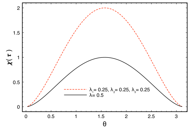
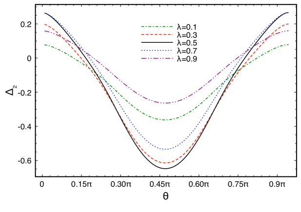
Note that $\chi(\tau)$ has periodicity $\pi$ with respect to $\theta$. It is straightforward to verify that the Holevo bound reaches its maximum value when $\theta=\pi/2$, corresponding to orthogonal spin states (see Fig. 1). At this point, and only at this point, it is possible for Bob to determine with certainty which state Alice has prepared, which he does simply by measuring $S_{z}$. This is actually a general property of orthogonal states, which can always be completely distinguished by appropriate measurements. By contrast, the minimum is attained at $\theta=0$ and $\theta=\pi$, which means that the states $\psi_{0}$ and $\psi_{1}$ are identical (up to a phase) when it comes solely to spin and, therefore, they cannot be distinguished at all.

Now, let us see how the above results generalize to the case where more classical bits are sent through the quantum communication channel. For this purpose, let us suppose now that Alice has a classical information source that produces symbols $\tilde{X}=00,01,10,11$ according to the probability distribution $p_{00}=\lambda_{1},p_{01}=\lambda_{2},p_{10}=\lambda_{3}$, $p_{11}=\lambda_{4}=1-\lambda_{1}-\lambda_{2}-\lambda_{3}$, $0\leq\lambda_{\tilde{l}}\leq 1,$ $\tilde{l}=1,2,3,4$. As in the previous case, Alice can choose pure quantum states from the set $\left\{\psi_{0},\psi_{1}\right\}$, where $\psi_{0}$ and $\psi_{1}$ are given by Eqs. (5) and (10), respectively. Therefore, depending on the value of $\tilde{X}$, Alice prepares one of the four product states

and sends it to Bob. He then makes a spin measurement of his choice on that state and has to identify $\tilde{X}$ based on the outcome $\tilde{Y}$. The total density operator of the system is given by

If the momentum degrees of freedom are traced out in Eq. (21), we obtain the reduced spin density operator

which can be written as

and from which all spin measurement results can be predicted. The density operators $\tau_{0}$ and $\tau_{1}$ are given in Eqs. (15) and (16), respectively. Now, by using that $S(\omega_{1}\otimes\omega_{2})=S(\omega_{1})+S(\omega_{2})$ for any density matrices $\omega_{1}$ and $\omega_{2}$ and that $S(\tau_{i})=0,$ we can write $\chi\left(\tilde{\tau}\right)$ as

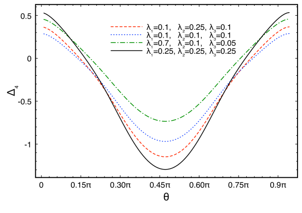
where $\tilde{\beta}_{\tilde{l}}$ are the eigenvalues of $\tilde{\tau}.$ In Fig 1, $\chi\left(\tilde{\tau}\right)$ is plotted when $\lambda_{1}=\lambda_{2}=\lambda_{3}=1/4$. We can see that, as in the case of two bits, its maximum value is attained when $\theta=\pi/2.$

Let us suppose first that Alice wants to transmit two bits of classical information. Thus, as explained in Section II.1, she prepares the state $\rho$ given in Eq. (13) and sends it to Bob. Due to his motion, Bob sees the state $\rho$ prepared by Alice unitarily transformed in his proper frame as

where Halpern1968 ; Weinberg1996

with

$p=\left(\sqrt{\mathbf{p}^{2}+m^{2}},\mathbf{p}\right)$, and $\Lambda^{-1}\mathbf{p}$ denoting the spatial part of the four-vector $\Lambda^{-1}p$. The Wigner rotation is given by

where $\alpha=-\tanh^{-1}v$, $q\equiv\Lambda^{-1}p,$ $\sigma^{0}=I$ is the identity matrix, and $\mathbf{e}$ gives the direction of the boost, which in our case is ${\bf e}_{x}$, so that

By using Eq. (27) in Eq. (26) with $\psi_{i}$ given in Eqs. (5) and (10), we obtain

and

where the momentum wave packets are given by

with

By tracing out the momentum degrees of freedom we obtain the reduced spin operator in Bob’s frame

where

and $\rho^{\prime}(\mathbf{p},\mathbf{p})$ is given in Eq (24). Explicitly, we have

where

with $V(\alpha)$ and $U(\alpha)$ being given by

and

respectively. In the above equations, we have used the fact that $\mbox{d}{\bf p}/p^{0}$ is a relativistic invariant and performed the change of variables $q=\Lambda^{-1}p$. Using Eqs. (36) and (39) in Eq (31), we can cast $\tau^{\prime}$ as

Note that, contrary to $\tau_{0}$ and $\tau_{1}$, $\tau_{0}^{\prime}$ and $\tau_{1}^{\prime}$ are not pure states, so that $S(\tau_{0}^{\prime})$ and $S(\tau_{1}^{\prime})$ are both non-zero. The Holevo bound in Bob’s frame is given by

By using Eqs. (36), (39) and (44), the above equation can be rewritten as

where, for $l=\pm$, $\gamma_{l}$, $\delta_{l}$, and $\epsilon_{l}$ are the eigenvalues of $\tau^{\prime}$, $\tau_{0}^{\prime}$, and $\tau_{1}^{\prime}$, respectively. These can be easily calculated as functions of the integrals $V(\alpha)$ and $U(\alpha)$. In this paper, we proceed a numerical analysis of Eq. (46) to examine various aspects of the transmission of classical information through relativistic quantum channels. In order to do that, we rewrite Eqs. (42) and (43) as

and

respectively, where we have used Eq. (11) and cylindrical coordinates with $q_{x}$ as the symmetry axis, and introduced

In addition, we have defined the normalized non-dimensional variables $Q_{r}\equiv q_{r}/m$, $Q_{x}\equiv q_{x}/m$, $Q^{0}=\sqrt{{Q_{x}}^{2}+{Q_{r}}^{2}+1}$, $W_{i}\equiv w_{i}/m$ and $K_{i}\equiv k_{i}/m$.

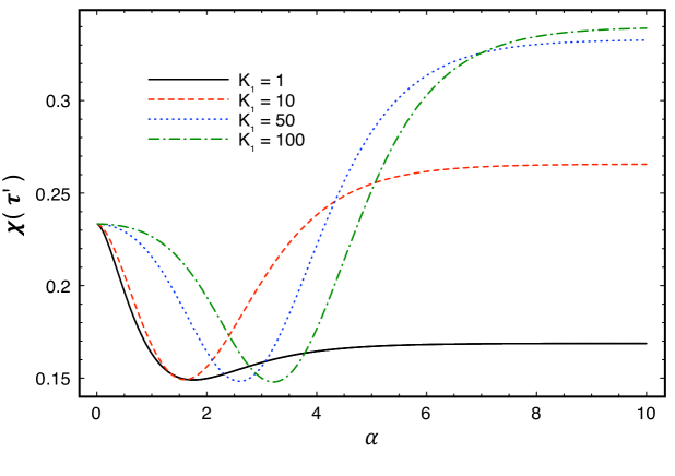
Let us first analyze the behavior of Eq (45) [or, equivalently, Eq (46)] as a function of the rapidity $\alpha=-\tanh^{-1}v,$ where we recall that $v$ is the relative velocity between Bob and Alice. First, it should be noted that if both $W_{0}$ and $W_{1}$ were much smaller than the unity, the effects of Bob’s velocity would be negligible and, for any value of $\alpha$, $\chi(\tau^{\prime})$ would have, approximately, its value for $\alpha=0$ (since in this case, $\psi_{0}$ and $\psi_{1}$ would be almost momentum eigenstates). However, if we allow $W_{1}$ to be much larger than $W_{0},$ the situation changes considerably, as can be seen in Fig. 2. There, $\chi(\tau^{\prime})$ is plotted as a function of the rapidity $\alpha$, for different values of the normalized mean momentum $K_{1}$ of $\psi_{1}$, when $W_{0}=0.05$, $W_{1}=6$, $\lambda=1/2$, $K_{0}=1$, and $\theta=\pi/8$. We can see that although $\chi(\tau^{\prime})$ initially decreases with $\alpha$, it begins to increase for larger values of the rapidity, eventually overcoming the value for $\alpha=0$ when $K_{1}$ is large enough. Thus, for some codifications, i.e., for some values of $\theta$, the (relativistic) velocity of the receiver can actually increase his accessible information. This is possible because, when $K_{1}$ is large, even though $W_{1}/W_{0}\approx 10^{2}$, the states $\psi_{0}$ and $\psi_{1}$ are almost orthogonal (despite of the fact that their spin parts, $\phi_{\uparrow}$ and $\phi_{\theta}$, are not), as can be easily checked. When Bob is moving, the momentum and spin degrees of freedom of the original state prepared by Alice are mixed up by the Wigner rotation. As a consequence, Bob can obtain some extra information in the spin degrees of freedom due to the fact that the states $\psi_{0}$ and $\psi_{1}$ prepared by Alice are more clearly distinguishable in momentum than in spin.

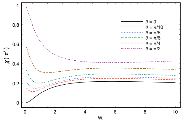
In view of the above results, let us study now how the width of the wave packet of the second state influences the accessible information in different codification schemes. In Fig. 3, $\chi(\tau^{\prime})$ is plotted as a function of $W_{1}$, in the limit $\alpha\rightarrow\infty$, for different values of $\theta$. We have fixed $W_{0}=0.05,$ $K_{0}=1,$ $K_{1}=10$, and $\lambda=1/2$. We can see that when $\theta$ is small and $W_{1}$ is large enough, the accessible information always increase when Bob moves with relativistic velocities with respect to Alice. When $\theta$ is larger (in particular, when it is close to $\pi/2$), the increase in $W_{1}$ always leads to a decrease in $\chi(\tau^{\prime})$ and therefore in the accessible information. This is so because the spin parts, $\phi_{\uparrow}$ and $\phi_{\theta},$ of the states $\psi_{0}$ and $\psi_{1}$ prepared by Alice are already quite distinguishable and thus the entanglement between the spin and momentum degrees of freedom caused by Bob’s movement ends up only making the spin degrees of freedom less distinguishable. It is interesting to note that Alice can codify the information in states $\psi_{0}$ and $\psi_{1}$ using $\theta=0$. This makes the states completely indistinguishable in spin in her frame. Yet, Bob can have a non zero value of $\chi(\tau^{\prime})$, as can be seen from Fig. 3. Thus, Alice can use the fact that spin and momentum are mixed up in Bob’s frame to “hide” the information in the momentum degrees of freedom in her frame, and let Bob movement make this information available to him in spin. This may be useful when considering noisy quantum channels in the spin degrees of freedom.

We will analyze now if the above results still apply when Alice sends more classical bits through the quantum channel. For the sake of simplicity, we will describe here what happens when she tries to transmit four bits of classical information to Bob. Thus, as explained in Section II.2, Alice prepares the state $\tilde{\rho}$ given in Eq. (21) and sends it to Bob. As Bob is moving with respect to her, he sees the state $\tilde{\rho}$ prepared by Alice unitarily transformed in his proper frame as

where $\psi^{\prime}_{ij}({\bf p},\tilde{{\bf p}})\equiv\psi^{\prime}_{i}({\bf p})\otimes\psi^{\prime}_{j}(\tilde{{\bf p}})$, $i,j=0,1$, and $\psi^{\prime}_{0}$ and $\psi^{\prime}_{1}$ are given in Eqs. (29) and (30), respectively. If we trace out the momentum degrees of freedom in $\tilde{\rho}^{\prime}\left(\mathbf{p},\mathbf{\tilde{p}},\mathbf{p}^{\prime},\mathbf{\tilde{p}}^{\prime}\right)$ we obtain the density operator

which can be written as

and from which all spin measurement results can be predicted. We recall that $\tau^{\prime}_{0}$ and $\tau^{\prime}_{1}$ are given in Eqs. (36) and (39), respectively.

Now, using again the identity $S(\omega_{1}\otimes\omega_{2})=S(\omega_{1})+S(\omega_{2})$, which is valid for any density matrices $\omega_{1}$ and $\omega_{2}$, we can write the Holevo bound

as

where $\tilde{\gamma}_{\tilde{l}},$ $\tilde{l}=1,2,3,4,$ are the eigenvalues of $\tilde{\tau}^{\prime}$.

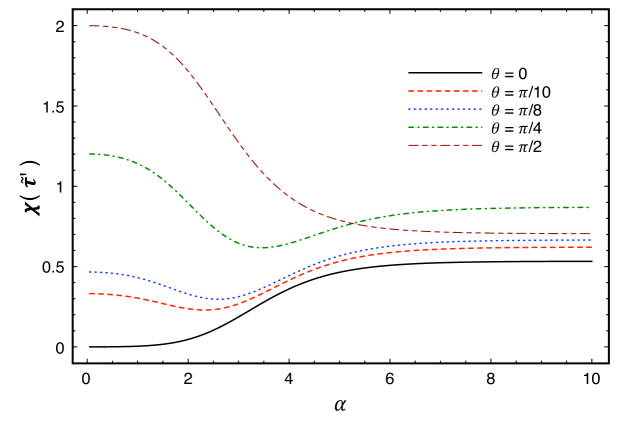
In Fig. 4 we plot $\chi(\tilde{\tau}^{\prime})$ as a function of the rapidity $\alpha$ for different values of the angle $\theta$. We have verified that the behavior of the Holevo bound for $\tilde{\tau}^{\prime}$ as a function of $\alpha$ for different values of $K_{1}$ is very similar to that of $\chi(\tau^{\prime})$, which is shown in Fig. 2. Similarly, the behavior $\chi(\tilde{\tau}^{\prime})$, when $\alpha\rightarrow\infty$, as a function of $W_{1}$ looks very close to the behavior of $\chi(\tau^{\prime})$ described in Fig. 3. Therefore, in order to analyze the Holevo bound for different choices of the angle $\theta$ of $\psi_{1}$, we have fixed $K_{1}$ and $W_{1}$ much larger than $K_{0}$ and $W_{0}$, respectively. Explicitly, we have chosen $K_{0}=1$, $K_{1}=50$, $W_{0}=0.05$, $W_{1}=6$, and $\lambda_{1}=\lambda_{2}=\lambda_{3}=\lambda_{4}=1/4.$ As can be seen from Fig. 4, $\chi(\tilde{\tau}^{\prime})$ initially decreases as $\alpha$ increases. However, for small angles (for instance, $\theta=0,$ $\theta=\pi/10$, and $\theta=\pi/8$), the Holevo bound begins to increase as $\alpha$ gets larger and, eventually, $\chi(\tilde{\tau}^{\prime})$ overcomes its value for $\alpha=0$ (where Bob is at rest with respect to Alice). Thus, for some codifications of the classical bits, the (relativistic) velocity of the receiver can increase his accessible information. For angles closer to $\pi/2,$ Bob’s movement only makes the Holevo bound smaller compared to the case where Alice and Bob do not have a relative motion. In particular, we can see from the graph that, when $\alpha$ is large enough, the use of orthogonal states, $\theta=\pi/2,$ is not even the best strategy anymore [i.e. orthogonal states do not maximize $\chi(\tilde{\tau}^{\prime})$]. Thus, for larger angles, it is better to use both $W_{0}$ and $W_{1}$ much smaller than $1$ so that $\psi_{0}$ and $\psi_{1}$ are “almost” momentum eigenstates and therefore, the effects of the motion of the receiver on the accessible information are negligible.

It is interesting to note that, as in the case where two bits are being sent through the quantum channel, Alice can “hide” the information on the momentum degrees of freedom by using states $\psi_{ij},$ $i,j=0,1$, with $\theta=0$ (which are completely indistinguishable in spin), and let Bob’s movement make the information available to him in the spin degrees of freedom. As we have already pointed out in Section III.1, this might be useful to protect the communication against possible noises in the spin degrees of freedom.