Sensing-Communication-Computing-Control Closed-Loop Optimization for 6G Unmanned Robotic Systems
Abstract
Rapid advancements in field robots have brought a new kind of cyber physical system (CPS)–unmanned robotic system–under the spotlight. In the upcoming sixth-generation (6G) era, these systems hold great potential to replace humans in hazardous tasks. This paper investigates an unmanned robotic system comprising a multi-functional unmanned aerial vehicle (UAV), sensors, and actuators. The UAV carries communication and computing modules, acting as an edge information hub (EIH) that transfers and processes information. During the task execution, the EIH gathers sensing data, calculates control commands, and transmits commands to actuators—leading to reflex-arc-like sensing-communication-computing-control () loops. Unlike existing studies that design loop components separately, we take each loop as an integrated structure and propose a goal-oriented closed-loop optimization scheme. This scheme jointly optimizes uplink and downlink (UL&DL) communication and computing within and across the loops to minimize the total linear quadratic regulator (LQR) cost. We derive optimal closed-form solutions for intra-loop allocation and propose an efficient iterative algorithm for inter-loop optimization. Under the condition of adequate CPU frequency availability, we derive an approximate closed-form solution for inter-loop bandwidth allocation. Simulation results demonstrate that the proposed scheme achieves a two-tier task-level balance within and across loops.
Index Terms:
Closed-loop optimization, goal-oriented communication, sensing-communication-computing-control () loop, unmanned robotic system, uplink and downlink (UL&DL) configurationI Introduction
I-A Background and Motivation
Cyber physical system (CPS) refers to the system that integrates communication, computing, and control to get information from the physical world, perform analysis, and change the physical world [1, 2]. In recent decades, a new kind of CPSs–unmanned robotic system–has received great attention for their human-like capabilities [3]. Driven by technologies such as smart computing and cloud-fog architectures, these systems have made significant strides in industrial automation, significantly improving production efficiency [4, 5]. Moreover, recent advancements in field robots have extended unmanned robotic systems from indoor factories to outdoor environments. These systems are now being deployed in hard-to-access areas, replacing humans in dangerous tasks such as disaster rescue [6], oil exploitation, and space exploration [7]. To fully unlock the potential of unmanned robotic systems, supporting field robots has been identified as an important use case for the sixth-generation (6G) network [nextG].
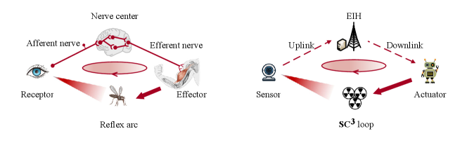
Due to the lack of ground facilities in remote areas, aerial-borne and space-borne platforms such as unmanned aerial vehicles (UAVs) and satellites, are envisioned to provide global seamless coverage in 6G [8, 9]. These platforms are agile to carry communication and computing modules, acting as edge information hubs (EIHs) to both transfer and process information [10]. A digital twin can be further integrated into EIHs to enable intelligent decision-making [11]. During the task execution, sensors collect raw data and upload them to the EIH via the sensor-EIH link. Based on the sensing data, the EIH calculates control commands. These commands are then transmitted to the actuators via the EIH-actuator link for actions. Synergistically, the sensor, the sensor-EIH link, the EIH, the EIH-actuator link, and the actuator form an integrated sensing-communication-computing-control () loop. Through effective feedback, the loop continuously learns the behavior of the physical system and guides its evolution to the desired direction. From the perspective of biology, the loop has great similarity to the reflex arc, as we compared in Fig. 1. In biology, it is widely recognized that the presence of the reflex depends on the functional integrity of the reflex arc [12]. In this sense, it is reasonable to take the loop as an integrated structure when we investigate the unmanned robotic system.
However, due to the heterogeneity of communication, computing, and control, current applications design -loop components separately. For this reason, the fifth-generation (5G) network positions itself as a communication network and primarily focuses on data transmission. It applies multiple access and duplex techniques, e.g., orthogonal frequency-division multiple access (OFDMA) and time-division duplexing/frequency-division duplexing (TDD/FDD), to decompose the network into independent links. Although this link-level division brings high capacity for communication, the task-level connections of different components within the loop are disintegrated. The mismatch of the sensor-EIH link, computing, and EIH-actuator link impairs the overall functioning of the loop, ultimately degrading the task efficiency of the robotic system.
Unlike Shannon who separated communication from its served system and regarded communication engineering as “reproducing at one point either exactly or approximately a message selected at another point” [13], the creator of cybernetics, Wiener, noted that “The problems of control engineering and communication engineering were inseparable, and that they centered not around the technique of electrical engineering but around the much more fundamental notion of the message.” [14]. By understanding communication through Wiener’s lens, we can find that communication is not merely for data transmission but an integral part for task execution. In this context, we need to shift our focus from individual communication links to integrated loops. As a result, the communication efficiency transcends bit transmission: it involves cooperating with computing and control to achieve good task performance. Building on these insights, we use a structured lens to regard the sensor and actuator within the loop as a virtual user [15]. The sensor-EIH link and EIH-actuator link are thus the uplink and downlink (UL&DL) of this virtual user. On this basis, we consider the goal-oriented closed-loop design for the unmanned robotic system.
I-B Related Studies
In the literature, related studies mostly focus on part of the loop. In wireless control systems (WCSs), the interplay between communication and control has been extensively studied. In mobile edge computing (MEC), joint optimization of communication and computing has been a central topic. In goal-oriented communication, related studies integrated the task efficiency into the communication design, and the learning-based approaches have become a dominant trend. In the following, we review related studies on WCS, MEC, and goal-oriented communication.
1) WCS: In WCS, related studies investigated the impact of imperfect communication, such as low data rate and latency, on control [16, 17]. From the theoretical perspective, Tatikonda et al. analyzed linear discrete-time systems and derived the lower and upper bounds on the data rate required for different control objectives [18]. Kostina et al. further generalized the work in [18] and derived the lower bound of the data rate given the control objective measured by the linear quadratic regulator (LQR) cost [19]. In terms of optimization schemes, Baumann et al. and Gatsis et al. devised control-aware transmission schemes that the sensor uploads sensing data only when the estimation error surpasses a certain threshold [20, 21]. By taking the LQR cost as the objective, Wang et al. optimized the UL [22], while Lei et al. and Fang et al. optimized the DL [23, 7]. For ultra-reliable and ultra-low latency communication (URLLC)-supported WCSs, Chang et al. jointly optimized communication bandwidth, power, and control convergence rate to maximize the spectrum efficiency (SE) [24], and Yang et al. optimized the UL&DL transmit power and block length to minimize a new metric named energy-to-control efficiency [25]. In addition to above theoretical advancements, researchers also established simulation platforms to testify the control performance under different communication conditions. Bhimavarapu et al. proposed a Unobtrusive Latency Tester solution to measure the communication latency and reliability in real-time control [26]. Lyu et al. proposed a novel hardware-in-the-loop simulation platform, which provided reliable test results by accurately stimulating the real wireless environment [27, 28]. Utilizing these platforms, the performance of 5G and Wi-Fi 6 was assessed, which provides valuable insights for selecting communication protocols for specific applications [26, 27, 28].
2) MEC: The core idea of MEC is to place computing resources close to mobile devices to support real-time applications. Most studies used joint communication and computing optimization to minimize the task latency [29, 30, 31], energy consumption [32][33], or maximize the utility [34, 35, 36]. For example, Wen et al. considered a TDD-mode MEC system in which each user is allocated a single slot to complete the data uploading, computing, and result downloading. The authors optimized bit, subchannel, and time allocation to minimize energy consumption [33]. Jian et al. focused on computing and DL transmission, proposing a joint MEC server-user association, CPU frequency, and bandwidth optimization scheme [34]. Wang et al. considered a joint sensing, communication, and computing framework, where the base station detects surrounding objects and uploads part of computing tasks to the cloud center using integrated sensing and communication (ISAC) signals. The authors optimized the beamformer and CPU frequency to maximize the computing rate [36].
3) Goal-Oriented Communication: The core idea of goal-oriented communication is to adapt communication strategies to the specific needs of supported tasks. For example, Wen et al. considered a real-time inference task performed by ISAC devices and an edge server. The authors took the discriminant gain as the objective and jointly optimized the transmit power, time allocation, and quantization bit allocation [37]. Girgis et al. proposed a semantic communication-control co-design that trains an encoder at the edge to abstract the low dimensional feature and a decoder at the control center to recover the state and calculate the command [38]. Shao et al. utilized the information bottleneck method to maximize the mutual information between the inference result and the encoded feature, while minimizing the mutual information between the raw input data and the encoded feature [39]. Mostaani et al. devised a distributed deep learning scheme for a multi-agent system, and maximized the long-term return by jointly optimizing communication and control policies [40].
In summary, these studies offer valuable insights into the design of the loop. Most of these studies have focused on part of the loop, such as UL and computing or DL and control, using indirect task metrics like latency or computing performance as their optimization objectives. However, for unmanned robotic systems, the reflex-arc-like loop is an integrated structure. The loop performance is reflected by the control actions on the physical world rather than the intermediate metrics. There is a lack of work that jointly optimizes the UL, computing, and DL within and across the loops from a goal-oriented perceptive.
I-C Main Contributions
In this paper, we consider an unmanned robotic system formed by a multi-functional UAV, sensors, and actuators. The UAV carries communication and computing modules, with a digital twin simulating the physical process in real time. During the task execution, the UAV acts as an EIH that collects data, calculates commands, and distributes commands to actuators to take actions. Together, the EIH, sensors, and actuators form reflex-arc-like loops. Different from current studies that devise loop components separately, our study takes the loop as an integrated structure and jointly configures UL, computing, and DL within and across the loops from a goal-oriented perspective. The main contributions are listed as follows.
-
1.
We investigate an unnamed robotic system formed by multiple reflex-arc-like loops. To effectively use limited resources, we propose a goal-oriented closed-loop optimization scheme that jointly optimizes bandwidth, time, and CPU frequency within and across loops, with the objective of minimizing the total LQR cost.
-
2.
In the intra-loop configuration, we derive optimal closed-form solutions for UL&DL bandwidth and time, along with the optimal LQR cost. Based on these results, we demonstrate the task-level balance between the UL&DL, as well as the interchange relationships between communication bandwidth and computing CPU frequency.
-
3.
In the inter-loop configuration, we propose an iterative algorithm to optimize the bandwidth and CPU-frequency allocation. Under the condition of adequate CPU frequency availability, we derive an approximate closed-form solution for the inter-loop bandwidth allocation and analyze the allocation principles regarding communication and control parameters.
-
4.
We conduct comprehensive simulation to validate our findings. We show the superiority of the goal-oriented closed-loop optimization by comparing it with separate schemes and communication-oriented schemes. We show that the proposed scheme achieves a two-tier task-level balance within and across the loops, which is crucial for the overall performance of the unmanned robotic system.
I-D Organization and Notation
The rest of this paper is organized as follows. Section II introduces the model of the unmanned robotic system and the related loop. Section III presents the goal-oriented closed-loop optimization scheme and its solution. Section IV presents simulation results and discussion. Section V draws conclusions.
Throughout this paper, vectors, matrices, and sets are represented by bold lowercase letters, bold uppercase letters, and curly uppercase letters, respectively. represents the set of real matrices, is the unit matrix, and is the zero matrix. denotes the eigenvalue of matrix and denotes the determinant of matrix . The complex Gaussian distribution of zero mean and variance is denoted as . The optimal solution of is denoted as .
II Unmanned Robotic System and Loop Model
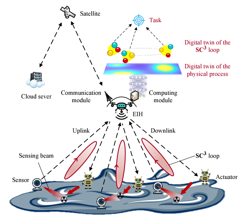
As shown in Fig. 2, we consider an unmanned robotic system performing a control-type task, such as radioactive object recycling. The system consists of loops, which are formed by a multi-functional UAV and pairs of sensors and actuators. The UAV carries communication and computing modules, serving as an EIH that transfers and processes information. A digital twin can be further integrated into the EIH for simulating the physical process in real time. We regard each pair of sensor and actuator as a virtual user. In this way, the sensor-EIH link and EIH-actuator link are the UL&DL of the virtual user. During the task execution, sensors collect raw data and upload them to the EIH via the UL. Based on the sensing data, the EIH updates the digital twin and calculates control commands using the reasoning of system behavior. These commands are transmitted to the actuators via the DL. Then, the actuators take actions. To ensure the correct operations of the EIH, the satellite provides telemetry, tracking, and control services for the EIH, while a cloud server provides high-level guidelines. In this paper, we focus on the unmanned robotic system in the field and do not consider the remote satellite and cloud server.
For simplicity, we assume that the controlled systems are linear time-invariant processes. For nonlinear processes, this linear model represents the linearization around the system’s working point, which provides a reasonable approximation of its local behavior [41]. Taking the -th loop and time index as an example, the system evolution is described by the following equation:
| (1) |
where denotes the system state, denotes the control action, denotes the process noise, and denotes the dimension of the controlled system. The matrices and are determined by the system dynamics, i.e., quantifies the intrinsic dynamics of the system without external intervention, and quantifies the effect of control actions on the state evolution. The system to be controlled is inherently unstable , and it can be stabilized by the pair . We use LQR cost to measure the control performance of the loop, which is a weighted summation of system states and control inputs over the entire control process,
| (2) |
where denotes the LQR cost, and are weighting matrices that balance the cost between state deviations and control inputs.
For communication, we denote the bandwidth, transmission time, and the SE of UL&DL as , , , , , and , respectively. According to the Shannon capacity, and are calculated as follows
| (3) | ||||
where and denote the channel gain, and denote the transmit power, is the channel noise variance. In this paper, we assume that the UL&DL SEs, and , remain constant throughout the control process. This can be achieved through adaptive power control, that the transmit power is dynamically adjusted according to channel conditions to maintain a target signal-to-noise ratio (SNR) [42]. This assumption applies to the bandwidth-constrained systems whose power resources are relatively sufficient to compensate for channel variations. By making this assumption, we focus on the bandwidth and time allocation in this paper. The channel gain consists of both small-scale fading and large-scale fading, which is given by,
| (4) | ||||
where and are the small-scale fading, which conforms to the complex Gaussian distribution, and and are the large-scale fading, which are calculated by the path-loss model,
| (5) | ||||
where (km) and (km) denote the transmission distance of the UL&DL, and (MHz) denotes the carrier frequency. In each cycle, the amount of information transmit via the UL&DL are given by,
| (6) | ||||
For computing, upon receiving sensing data, the EIH processes these data, extracts task-related information, and updates the digital twin. Using the updated digital twin, which simulates system behavior, the EIH calculates control commands. The information extraction process is described as,
| (7) |
where is a proportion parameter. denotes the task-related information extracted from the sensing data, which also denotes the information contained in the command. The computing time is calculated by,
| (8) |
where (cycles/bit) denotes the processing difficulty (the required CPU cycles for processing one-bit data), denotes the allocated CPU frequency for the -th loop, and we denote . In practice, and are the parameters of the neural network . A larger network usually provides a more accurate modeling of the physical process, enables a more thorough extraction of task-related information, and outputs more effective control commands, resulting in a higher . Conversely, the larger network also incurs greater computational complexity, resulting in a higher . Therefore, finding a proper precision of the digital twin is crucial for the practical deployment [43]. Nonetheless, we do not delve into this issue in this paper. The calculated commands are sent to the actuators to guide their actions. However, due to the capacity constraints of the DL, the command information may not fully reach the actuators. The information that finally works for the controlled system is jointly determined by the task-related information extracted from the UL and the information successfully transmitted via the DL,
| (9) |
where is defined as the closed-loop information, which is the information that finally works within one cycle. According to [19], the lower bound of the LQR cost has a direct relationship with the closed-loop information as,
| (10) |
where and is the differential entropy of , i.e., , is the covariance matrix of the process noise, is the intrinsic entropy, and and are determined by the Riccati equations,
| (11) | ||||
To ensure the system can be stabilized, the closed-loop information needs to satisfy the following stable condition [19],
| (12) |
In addition, the loop needs to run within the given cycle time, and we have the following cycle-time constraint,
| (13) |
where denotes the cycle time for the -th loop. We can see from (9) and (10), the LQR cost is constrained by the closed-loop information, and the closed-loop information is further determined by the information transmitted via the UL&DL. In addition, the computing time affects the time available for data transmission, thereby indirectly influencing the LQR cost. Consequently, a co-design of UL, computing, and DL is essential to ensure a good control performance of the loop.
III Goal-Oriented Closed-Loop Optimization
III-A Problem Formulation
In this paper, we aim to minimize the total LQR cost of the unmanned robotic system by jointly optimizing bandwidth, CPU frequency, and time within and across the loops. The optimization problem is formulated as follows:
| (P1) | (14a) | |||
| s.t. | (14b) | |||
| (14c) | ||||
| (14d) | ||||
| (14e) | ||||
| (14f) | ||||
| (14g) | ||||
| (14h) | ||||
| (14i) | ||||
| (14j) | ||||
where and denote the maximal bandwidth and CPU frequency, respectively. Due to the coupling relationships among different variables, (P1) is a highly complex problem with non-convex constraints (14e), (14f) and (14g). To address this challenge, we begin by investigating the intra-loop configuration within an loop and move to investigate the inter-loop optimization across multi- loops.
III-B Single--Loop Optimization
For simplicity, the index is omitted when we consider an loop. When , the optimization problem becomes
| (PA-1) | (15a) | |||
| s.t. | (15b) | |||
| (15c) | ||||
| (15d) | ||||
| (15e) | ||||
| (15f) | ||||
| (15g) | ||||
| (15h) | ||||
| (15i) | ||||
| (15j) | ||||
As the lower bound of the LQR cost (15b) monotonically decreases with the closed-loop information, minimizing the LQR cost is equivalent to maximizing the closed-loop information for an loop. In addition, as there are no other loops competing for resources, the optimal CPU frequency is its maximum allowable value, i.e., . As a result, the critical focus in the single--loop optimization is the UL&DL configuration,
| (PA-2) | (16a) | |||
| s.t. | (16b) | |||
| (16c) | ||||
| (16d) | ||||
| (16e) | ||||
| (16f) | ||||
| (16g) | ||||
where the stable condition (15d) is omitted. We test it after solving (PA-2). If the optimization result, satisfies (15d), we calculate the LQR cost according to (10). Otherwise, the controlled system cannot be stabilized, and the LQR cost is infinite.
Lemma 1:
The optimal UL&DL configuration for an loop is to keep a task-level balance, described by the following equation,
| (17) |
The optimal UL&DL time allocation is given by,
| (18) | |||
Proof:.
See Appendix A.
From (17), we can see that the task-level balance between UL&DL is to match the task-related information extracted from the raw data transmitted via the UL with the information transmitted via the DL. This balance can be illustrated by the analogy to water pipes. The UL and computing are considered as one pipe, while the DL is another. Just as the maximum water flow through the interconnected pipes is limited by the pipe with the smallest capacity, the optimal solution requires equalizing the capacities of both pipes, as indicated by the equilibrium in (17).
Based on the (17) and (18), we can express the closed-form information as an expression of the bandwidth,
| (19) | ||||
From (19), we observe that is monotonically decreasing with . This expression represents the time to transfer or process one-bit task-related information, where , , and represent the time for UL, computing, and DL, respectively. Therefore, we move to consider the time-minimization problem as follows:
| (20a) | ||||
| s.t. | (20b) | |||
| (20c) | ||||
Theorem 1:
The optimal UL&DL bandwidth allocation is given by:
| (21a) | ||||
| (21b) | ||||
The optimal closed-loop information and optimal LQR cost are given by:
| (22) |
| (23) |
where denotes the SE of the loop, referred to as closed-loop SE, and denotes the computing efficiency (CE):
| (24a) | ||||
| (24b) | ||||
Proof:.
See Appendix B.
From (24a), we can see that the closed-loop SE is jointly determined by the UL&DL SEs. It has the following approximation,
| (25) |
In fact, and represent the task-level SE of UL&DL, respectively. From (25), we can learn that closed-loop SE is determined by the weak link. A task-level balance of UL&DL SEs is required to ensure a large closed-loop SE.
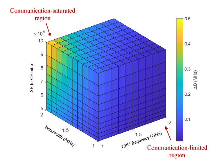
In addition, from (22), we observe an interesting trade-off between bandwidth and CPU frequency for a given closed-loop performance. This trade-off is achieved by adjusting communication and computing time. For instance, increasing the bandwidth reduces communication time, , which in turn allows for an increase in computing time, , leading to a reduction of the CPU frequency. Consequently, the relationship between and can be derived to illustrate how bandwidth and CPU frequency can be exchanged for a given closed-loop performance:
| (26) | ||||
From the above expression, we observe that is influenced by the working point of the loop, characterized by the bandwidth, CPU frequency, and SE-to-CE ratio, . With a fixed , a large bandwidth is required when is high, is low, and is high, which corresponds to the communication-saturated region.
III-C Multi--Loop Optimization
Based on the optimal intra-loop configuration, we move to the inter-loop allocation problem. Using the optimal LQR cost expression (23), (P1) is simplified into the following inter-loop bandwidth and CPU frequency allocation problem:
| (PB-1) | (27a) | |||
| s.t. | (27b) | |||
| (27c) | ||||
| (27d) | ||||
| (27e) | ||||
| (27f) | ||||
| (27g) | ||||
where denotes the bandwidth allocated to the -th loop and we denote . By calculating the second-order derivative of the right-hand side of (27b), it is easy to prove that it is a convex expression of . Thus, the only non-convex constraint in (PB-1) is (27c). To address this, we first transform it into
| (28) |
Since is a convex expression of when , we can see that only the right-hand side of (28) does not satisfy the rule of convex optimization. By using the successive convex approximation, we propose an iterative algorithm. The convex optimization problem in the -th iteration is given by
| (PB-2) | (29a) | |||
| s.t. | (29b) | |||
| (29c) | ||||
where the right side of (29c) is the Taylor expansion of at the result obtained in the -th iteration, . We summarize the proposed iterative algorithm in Algorithm 1. The convergence of the algorithm is proved in Appendix C.
Next, we derive the approximate closed-form solution for the inter-loop bandwidth allocation. We assume that the CPU frequency is sufficiently adequate such that the computing time becomes negligible compared to the communication time, . On this basis, the LQR cost can be approximated as follows:
| (30) |
where the term [] in the denominator is omitted from its original expression (23), under the assumption that the system operates in the assured-to-be-stable region, i.e., . Using (30), (PB-1) is simplified into a convex bandwidth allocation problem,
| (31a) | ||||
| s.t. | (31b) | |||
| (31c) | ||||
where is omitted as it does not influence the allocation results. The stable condition is also omitted as in the assure-to-be-stable region.
Theorem 2:
The optimal bandwidth allocation to (PB-3) is given by
| (32) | ||||
where denotes the control-related parameter,
| (33) |
Proof:.
See Appendix D.
We can learn from (32) that bandwidth allocation is influenced by both the communication parameter, , and the control parameter, . The loop with poor communication performance (smaller ) or controlling a more unstable system (larger ) is allocated more bandwidth. This shows that this inter-loop bandwidth allocation is fairness-minded, which balances the control processes across different loops.
IV Simulation Results and Discussion
In this section, we present the simulation results and discussion. We consider an unmanned robotic system composed of loops. The channel noise variance is dBm [44], and the large-scale fading coefficients, and , are calculated using the path-loss model given in (5), where GHz, and UL&DL distances are set as km and km, respectively. The small-scale fading is randomly generated following [44]. The UL&DL transmit power is adjusted to maintain a constant received SNR, i.e., and . Accordingly, we can calculate the UL&DL SEs by (3), i.e, bits/s/Hz and bits/s/Hz. The computing-related parameters are set as GHz, , , and (cycles/bit). The control-related parameters are configured as , , , [7], and ms, . The iteration termination threshold is set as , and the optimization tool is CVX [45]. Unless otherwise stated, these parameters are used throughout the results below.
IV-A Single--Loop Simulation
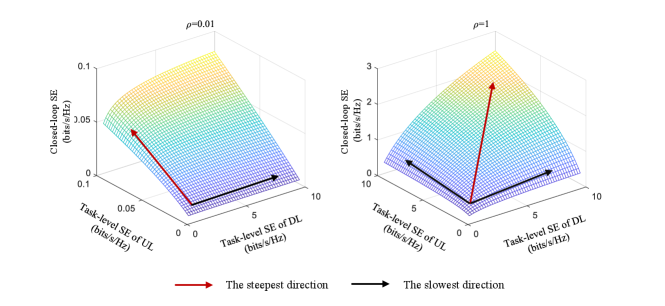
In Fig. 3, we present the relationships between UL&DL SEs and the closed-loop SE, as described in (25). In the left figure, we set the information extraction ratio as , which creates the unbalance of UL&DL SEs at the task level. In this case, the closed-loop SE is constrained by the UL. As indicated by the red and black arrows, the most effective way to enhance the closed-loop SE is by improving the UL SE, while improving the DL SE provides little improvement. In contrast, the right figure illustrates the case where the information extraction ratio is set as , resulting in relatively balanced task-level UL&DL SEs. In this case, the most effective way to enhance the closed-loop SE is to simultaneously improve UL&DL SEs. It is noted that, in practice, the raw data transmitted via the UL often contain redundant and irrelevant information, leading the information extraction ratio a very small number, . An enhanced UL is usually required for keeping the task-level balance between UL&DL.
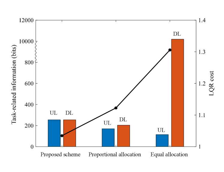
In Fig. 4, we present the LQR cost under different UL&DL configurations. Here, we compare the proposed scheme with two classical schemes: equal allocation and proportional allocation.
-
•
Equal allocation: The bandwidth is equally divided for UL&DL like FDD, .
-
•
Proportional allocation: The UL&DL bandwidth is proportional allocated per the information extraction ratio, and .
In above two schemes, the DL transmission time is set as , and the remaining time is adjusted between UL and computing by letting the UL transmitted information rightly processed by computing, i.e., . The maximal bandwidth is set as kHz, and the CPU frequency is set as GHz. Fig. 4 is a dual-axis chart with the left side representing the task-related information and the right side representing the LQR cost. From the bar, we can see that, under the proposed scheme, the UL&DL are aligned to transmit the same amount of task-related information, while the other two schemes fail to achieve this balance. Their weak ULs constrain the control performance of the loop, leading to the high LQR cost (shown by the black curve). In addition, we can observe that the LQR cost is higher with more degree of UL&DL imbalance, indicating the importance of keeping task-level UL&DL balance within the loop.
In Fig. 5, we illustrate the interchange relationships between bandwidth and CPU frequency. This figure shows the required bandwidth in exchange for 1 MHz CPU frequency under different working points of the loop, described by the bandwidth, CPU frequency, and SE-to-CE ratio, i.e., (, ,). The color gradient represents the amount of required bandwidth, increasing as the color shifts from blue to yellow. The figure shows that in the communication-saturated region, more bandwidth is required compared to the communication-limited region. For example, at the working point of , the required bandwidth is , whereas at , the required bandwidth is , with an increase of forty-fold. This indicates the marginal effect, that the effectiveness of additional bandwidth diminishes as the loop approaches the communication-saturated region.
IV-B Multi--Loop Simulation
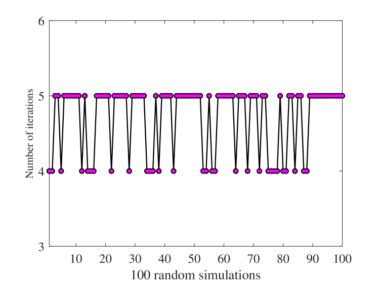
In Fig. 6, we provide the convergence performance of the proposed iterative algorithm. In this simulation, we randomly generate UL&DL distances within the range of km, the maximum bandwidth is set as MHz. The results show that, across all 100 simulations, the proposed algorithm consistently requires only 4 or 5 iterations to converge.
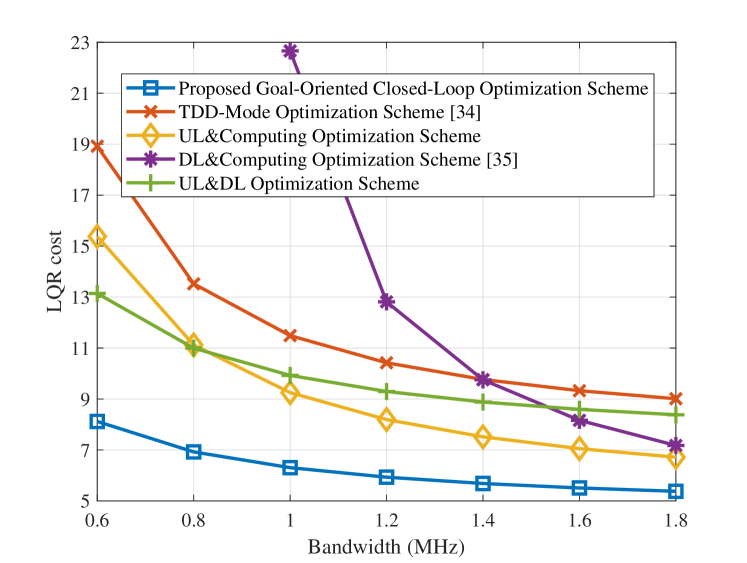
In Fig. 7 we compare the proposed scheme with a TDD-mode optimization scheme [33] and three separate schemes, with each focused on a part of the loop. For fair comparisons, we consider these schemes to be goal-oriented by taking the LQR cost as the objective.
-
•
TDD-Mode Optimization Scheme [33]: This scheme uses TDD to access four loops. Each loop is allocated with an equal time slot, ms, and exclusively uses bandwidth and CPU frequency resources in this slot. It optimizes the UL&DL, and computing time for each loop.
-
•
UL&Computing Optimization Scheme: This scheme optimizes UL transmission and computing, while the DL parameters are fixed as and .
-
•
DL&Computing Optimization Scheme [34]: This scheme optimizes DL transmission and computing, with the UL parameters fixed at and .
-
•
UL&DL Optimization Scheme: This scheme optimizes UL&DL transmission, with the CPU frequency fixed at .
It can be observed that the proposed scheme achieves the lowest LQR cost compared to the other four schemes. In the bandwidth-limited region, the DL&Computing Optimization Scheme [34] performs the worst. This is because the fixed UL is the bottleneck, which largely determines the -loop performance: the data transmitted via the UL are the data processed by computing, which in turn determines the accuracy of the command transmitted via the DL. Conversely, in the bandwidth-adequate region, the TDD-Mode Optimization Scheme and UL&DL Optimization Scheme perform poorly. This is because these two schemes constrain the inter-loop adjustment, negatively affecting the balance of the control progress across different loops. This highlights the advantage of treating the loop as an integrated structure and jointly configuring resources within and across the loops.
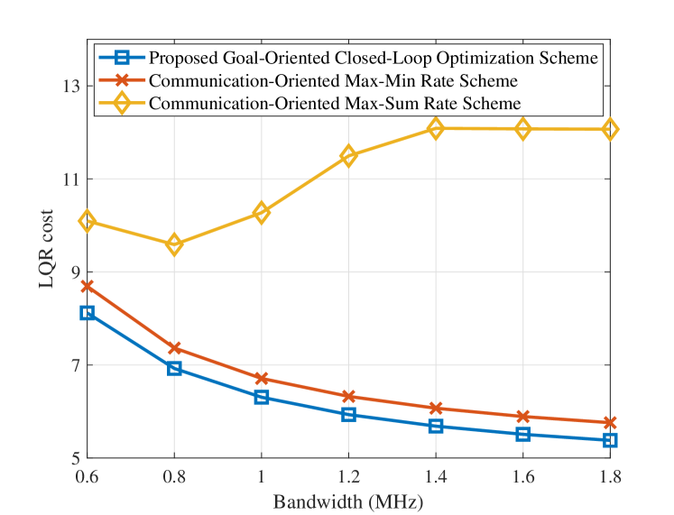
In Fig. 8, we compare the proposed goal-oriented scheme with two communication-oriented schemes.
-
•
Communication-Oriented Max-Sum Rate Scheme: This scheme maximizes the sum of the closed-loop information, i.e., .
-
•
Communication-Oriented Max-Min Rate Scheme: This scheme maximizes the minimal closed-loop information, i.e., .
These two communication-oriented schemes can be solved using a similar iterative algorithm by replacing the objective of the LQR cost with the sum-rate and min-rate objective, i.e., and , and convert the LQR constraint (29b) into a closed-loop-information constraint,
| (34) |
In this simulation, we set the LQR cost requirement in (34) as . From the figure we can see that, the Communication-Oriented Max-Sum Rate Scheme performs the worst. This is because this scheme disproportionately allocates the most resources to the loops with the highest SE and CE, amplifying the imbalance among different loops. As the bandwidth increases, this bias intensifies, leading the LQR cost of other loops to rise sharply, resulting in the increase of the sum LQR cost. In addition, we can observe that, when MHz, the LQR cost reaches its maximum and remains unchanged under the Communication-Oriented Max-Sum Rate Scheme. In this region, the control performance of the loops diverges into two extremes: the LQR cost of the loops with the highest SE or CE approaches its minimal value, while the LQR cost of the remaining loops barely meets the basic requirement as given in (34). Conversely, the Communication-Oriented Max-Min Rate Scheme performs similarly to the proposed scheme. They have a small performance gap, which is because the Max-Min Rate Scheme prioritizes the rate balance while overlooking the differences of controlled systems. The good performance of the Max-Min Rate Scheme and the proposed scheme indicates the importance of keeping balance across different loops.
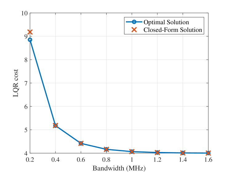
Fig. 9 compares the approximate closed-form solution for the inter-loop bandwidth allocation (32) with the optimal solution obtained by CVX. We can see that the LQR costs under the approximate closed-form solution and the optimal solution exhibit a small gap in the bandwidth-limited region, and this gap rapidly approaches zero as the bandwidth increases. This demonstrates the accuracy of the approximate closed-form solution, particularly when the system has sufficient communication and computing resources.
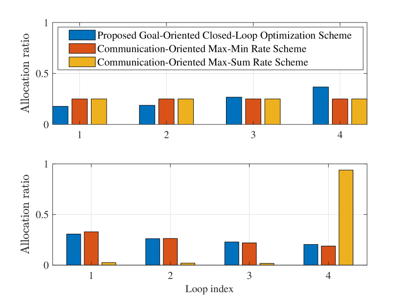
Furthermore, we show the bandwidth allocation principles by comparing the proposed goal-oriented scheme with two communication-oriented schemes in Fig. 10. The maximal bandwidth is set as MHz. In the top subfigure, we set the four loops with different intrinsic entropy, , and equal SE, bits/s/Hz, . It can be seen that the proposed scheme allocates more bandwidth to the loops with higher intrinsic entropy, whereas two communication-oriented schemes allocate bandwidth equally. This is because the communication-oriented schemes focus on the data rate, and as a result, they are unable to perceive the stability differences of the controlled systems. In the bottom subfigure, we set the four loops with different SEs, bits/s/Hz, and equal intrinsic entropy, . In this case, the Max-Sum Rate Scheme disproportionately allocates the most resources to the loop with the highest SE (loop 4), leaving other loops with minimal resources to satisfy the LQR-cost constraint (34). In contrast, both the proposed scheme and the Max-Min Rate Scheme allocate more bandwidth to the loops with lower SEs, aiming to achieve the task-level and rate-level balance, respectively. This shows that the proposed scheme is fairness-minded. Instead of over-resourcing the strong loop at the expense of others, it maintains the task-level balance across loops to ensure the control performance of the whole unmanned robotic system.
V Conclusions
In this paper, we have investigated an unmanned robotic system formed by the reflex-arc-like loops. We have proposed a goal-oriented closed-loop optimization scheme that jointly configures UL&DL bandwidth, time, and CPU frequency to improve the control performance of the system. We have derived closed-form solutions for the UL&DL bandwidth and time allocation within the loop and proposed an iterative algorithm to optimize the inter-loop bandwidth and CPU frequency allocation. Under the condition of adequate CPU frequency availability, we have also derived the approximate closed-form solution for the inter-loop bandwidth allocation. We have shown that the superiority of the proposed scheme lies in achieving a two-tier task-level balance within and across the loops. We believe that such a structured design—taking the loop as an integrated structure—will promote the development of unmanned robotic systems in 6G.
Appendix A Proof of Lemma 1
In (PA-2), the optimal values of , , and are their maximum value allowed. As a result, the equality in constraints (16b)–(16d) must hold at the optimal solution,
| (35) |
where
| (36) |
If at the optimal solution, taking as an example, we thus have . In this case, can be improved by reallocating UL time to the DL as long as . This improves the objective by
| (37) |
which contradicts the assumption that is optimal. Similarly, if , we can use the similar reasoning to show that can be improved. Therefore, neither nor hold, meaning that at the optimal solution .
Furthermore, based on , we have . The optimal time for DL transmission and computing can be expressed as a function of the optimal time for UL transmission,
| (38) |
In addition, since more time enables transmitting and processing more information, thereby increasing , the cycle-time constraint (16e) must be satisfied as an equality at the optimal solution,
| (39) |
Then by substituting (38) into (39), we obtain the optimal expression of the UL transmission time,
| (40) | |||||
Based on , we can further obtain and by substituting (40) into (38).
Appendix B Proof of Theorem 1
In (PA-3), the objective is monotonically decreasing with the UL&DL bandwidth. Therefore, the bandwidth constraint (20b) must be satisfied as an equality at the optimal solution,
| (41) |
We let and substitute it to the objective. By calculating the first-order derivative of the objective and setting it to zero, we derive the optimal closed-form solution for the bandwidth allocation as follows:
| (42) | ||||
Then, it is easy to further get according to (41). By substituting and into (19) and (10), we further get the optimal expression of the closed-form information, , and LQR cost, .
Appendix C Proof of the convergence of Algorithm 1
We prove the convergence of the proposed algorithm by proving this optimization process leads to a non-increasing objective. We first prove that the solution in the -th iteration is a feasible solution in the -th iteration.
From convenience, we introduce a function to express the constraint (29c) in (PB-2),
| (43) |
Denote the results obtained in the -th iteration as . The constraint (29c) in the -th iteration can be expressed as
| (44) |
where represents the Taylor expansion of at . Since is a concave expression for when , its Taylor expansion is greater than or equal to the original value. Therefore, we have the following inequalities:
| (45) | ||||
This shows that is a feasible solution in the -th iteration. As a result, is an achievable objective in the -th iteration. Since in the -th iteration, is the optimal solution, it satisfies that . According to the monotone bounded theorem, the proposed iterative algorithm is assured to be convergent.
Appendix D Proof of Theorem 2
(PB-3) is a convex optimization problem and satisfies the Slater condition, which guarantees strong duality. As a result, the optimal solution to the dual problem is the same as that of the primal problem. Therefore, we solve the dual problem of (PB-3) to obtain the closed-form solution for the bandwidth. The dual problem is formulated as follows:
| (46a) | ||||
| s.t. | (46b) | |||
where is the Lagrange multiplier. The Karush-Kuhn-Tucker (KKT) condition of (PB-4) is given by
| (47a) | |||
| (47b) | |||
| (47c) | |||
| (47d) | |||
where the constraint (47b) is an equality since the available bandwidth must be fully utilized at the optimal solution. By calculating (47a), the optimal bandwidth is expressed as a function of ,
| (48) |
We further substitute (48) into (47b) to get the following expression of the Lagrange multiplier,
| (49) | ||||
By back-substituting the above expression into (48), we thus obtain the closed-form solution for the inter-loop bandwidth allocation, as given in (32) in Theorem 2.
References
- [1] E. A. Lee, “The past, present and future of cyber-physical systems: A focus on models,” Sensors, vol. 15, no. 3, pp. 4837-4869, Feb. 2015.
- [2] H. Chen “Applications of cyber-physical system: A literature review,” J. Ind. Integr. Manage., vol. 2, no. 3, pp. 1750012, Qct. 2017.
- [3] P. Jain, P. K. Aggarwal, P. Chaudhary et al., “Convergence of IoT and CPS in robotics,” Emergence of Cyber Physical System and IoT in Smart Automation and Robotics, Cham, Springer Int. Publ., 2021.
- [4] H. Lyu, J. Yan, J. Zhang, Z. Pang, G. Yang, and A. J. Isaksson, “Cloud–fog automation: Heterogenous applications over new-generation infrastructure of virtualized computing and converged networks,” IEEE Ind. Electron. Mag., Early Access, Jun. 2024.
- [5] J. Jin, K. Yu, J. Kua, N. Zhang, Z. Pang, and Q. -L. Han, “Cloud-fog automation: Vision, enabling technologies, and future research directions,” IEEE Trans. Ind. Inf., vol. 20, no. 2, pp. 1039-1054, Feb. 2024.
- [6] R. Mariappan, P. V. Narayana Reddy, and C. Wu, “Cyber physical system using intelligent wireless sensor actuator networks for disaster recovery,” in Proc. 2015 Int. Conf. Comput. Intell. Commun. Netw. (CICN), Jabalpur, India, 2015, pp. 95-99.
- [7] X. Fang, W. Feng, Y. Chen, N. Ge, and G. Zheng, “Control-oriented deep space communications for unmanned space exploration,” IEEE Trans. Wireless Commun., Early Access, Jun. 2024.
- [8] X. Fang, W. Feng, T. Wei, Y. Chen, N. Ge, and C. -X. Wang, “5G embraces satellites for 6G ubiquitous IoT: Basic models for integrated satellite terrestrial networks,” IEEE Internet Things J., vol. 8, no. 18, pp. 14399-14417, Sep. 2021.
- [9] W. Feng, Y. Lin, Y. Wang, J. Wang, Y. Chen, N. Ge, S. Jin, and H. Zhu, “Radio map-based cognitive satellite-UAV networks towards 6G on-demand coverage,” IEEE Trans. Cognit. Commun. Netw., vol. 10, no. 3, pp. 1075-1089, Jun. 2024.
- [10] C. Lei, W. Feng, P. Wei, Y. Chen, N. Ge, and S. Mao, “Edge information hub: Orchestrating satellites, UAVs, MEC, sensing and communications for 6G closed-loop controls,” IEEE J. Sel. Areas Commun., Early access, Sep. 2024.
- [11] D. Jones, C. Snider, A. Nassehi, et al., “Characterising the digital twin: A systematic literature review,” CIRP J. Manuf. Sci. Technol., vol.29, pp. 36-52, May 2020.
- [12] A. Rijnberk and H. W. (Eds.) De Vries, “Medical history and physical examination in companion animals,” Springer Science & Business Media, 1995.
- [13] C. E. Shannon, “A mathematical theory of communication,” The Bell Sys. Tech. J., vol. 27, no. 3, pp. 379-423, Jul. 1948.
- [14] N. Wiener, “Cybernetics: Or control and communication in the animal and the machine,” MIT press, 2019.
- [15] W. Feng, Y. Wang, Y. Chen, N. Ge, and C.-X. Wang, “Structured satellite-UAV-terrestrial networks for 6G Internet of Things,” IEEE Netw., vol. 38, no. 4, pp. 48-54, Jul. 2024.
- [16] P. Park, S. Coleri Ergen, C. Fischione, C. Lu, and K. H. Johansson, “Wireless network design for control systems: A survey,” IEEE Commun. Surv. Tutorials, vol. 20, no. 2, pp. 978-1013, Q2nd 2018.
- [17] Y. Wang, S. Wu, C. Lei, J. Jiao, and Q. Zhang, “A review on wireless networked control system: The communication perspective,” IEEE Internet Things J., vol. 11, no. 5, pp. 7499-7524, Mar. 2024.
- [18] S. Tatikonda and S. Mitter, “Control under communication constraints,” IEEE Trans. Autom. Control, vol. 49, no. 7, pp. 1056-1068, Jul. 2004.
- [19] V. Kostina and B. Hassibi, “Rate-cost tradeoffs in control,” IEEE Trans. Autom. Control, vol. 64, no. 11, pp. 4525-4540, Nov. 2019.
- [20] D. Baumann, F. Mager, M. Zimmerling, and S. Trimpe, “Control-guided communication: Efficient resource arbitration and allocation in multi-hop wireless control systems,” IEEE Control Sys. Lett., vol. 4, no. 1, pp. 127-132, Jan. 2020.
- [21] K. Gatsis, A. Ribeiro, and G. J. Pappas, “Optimal power management in wireless control systems,” IEEE Trans. Autom. Control, vol. 59, no. 6, pp. 1495-1510, Jun. 2014.
- [22] X. Wang, C. Chen, J. He, S. Zhu, and X. Guan, “AoI-aware control and communication co-design for industrial IoT systems,” IEEE Internet Things J., vol. 8, no. 10, pp. 8464-8473, May 2021.
- [23] C. Lei, W. Feng, J. Wang, S. Jin, and N. Ge, “Control-oriented power allocation for integrated satellite-UAV networks,” IEEE Wireless Commun. Lett., vol. 12, no. 5, pp. 883-887, May 2023.
- [24] B. Chang, L. Zhang, L. Li, G. Zhao, and Z. Chen, “Optimizing resource allocation in URLLC for real-time wireless control systems,” IEEE Trans. Veh. Technol., vol. 68, no. 9, pp. 8916-8927, Sep. 2019.
- [25] H. Yang, K. Zhang, K. Zheng, and Y. Qian, “Leveraging linear quadratic regulator cost and energy consumption for ultrareliable and low-latency IoT control systems,” IEEE Internet Things J., vol. 7, no. 9, pp. 8356-8371, Sep. 2020.
- [26] K. Bhimavarapu, Z. Pang, O. Dobrijevic, and P. Wiatr, “Unobtrusive, accurate, and live measurements of network latency and reliability for time-critical internet of things,” IEEE Internet Things Mag., vol. 5, no. 3, pp. 38-43, Sep. 2022.
- [27] H. Lyu, Z. Pang, K. Bhimavarapu, and G. Yang, “Impacts of wireless on robot control: The network hardware-in-the-loop simulation framework and real-life comparisons,” IEEE Trans. Ind. Inf., vol. 19, no. 9, pp. 9255-9265, Sep. 2023.
- [28] H. Lyu, Z. Pang, A. Bengtsson, S. Nilsson, A. J. Isaksson, and G. Yang, “Latency-aware control for wireless cloud-fog automation: Framework and case study,” IEEE Trans. Autom. Sci. Eng., Early Access, Jul. 2024.
- [29] J. Liu and Q. Zhang, “Offloading schemes in mobile edge computing for ultra-reliable low latency communications,” IEEE Access, vol. 6, pp. 12825-12837, Feb. 2018.
- [30] L. Ferdouse, A. Anpalagan, and S. Erkucuk, “Joint communication and computing resource allocation in 5G cloud radio access networks,” IEEE Trans. Veh. Technol., vol. 68, no. 9, pp. 9122-9135, Sep. 2019.
- [31] C.-L. Chen, C. G. Brinton, and V. Aggarwal, “Latency minimization for mobile edge computing networks,” IEEE Trans. Mob. Comput., vol. 22, no. 4, pp. 2233-2247, Apr. 2023.
- [32] X. Cao, F. Wang, J. Xu, R. Zhang, and S. Cui, “Joint computation and communication cooperation for energy-efficient mobile edge computing,” IEEE Internet Things J., vol. 6, no. 3, pp. 4188-4200, Jun. 2019.
- [33] W. Wen, Y. Fu, T. Q. S. Quek, F. -C. Zheng, and S. Jin, “Joint uplink/downlink sub-channel, bit and time allocation for multi-access edge computing,” IEEE Commun. Lett., vol. 23, no. 10, pp. 1811-1815, Oct. 2019.
- [34] Z. Jian, W. Muqing, and Z. Min, “Joint computation offloading and resource allocation in C-RAN with MEC based on spectrum efficiency,” IEEE Access, vol. 7, pp. 79056-79068, Jun. 2019.
- [35] S. Li, S. Lin, L. Cai, W. Li, and G. Zhu, “Joint resource allocation and computation offloading with time-varying fading channel in vehicular edge computing,” IEEE Trans. Veh. Technol., vol. 69, no. 3, pp. 3384-3398, Mar. 2020.
- [36] Z. Wang, X. Mu, Y. Liu, X. Xu, and P. Zhang, “NOMA-aided joint communication, sensing, and multi-tier computing systems,” IEEE J. Sel. Areas Commun., vol. 41, no. 3, pp. 574-588, Mar. 2023.
- [37] D. Wen et al., “Task-oriented sensing, computation, and communication integration for multi-device edge AI,” IEEE Trans. Wireless Commun., vol. 23, no. 3, pp. 2486-2502, Mar. 2024.
- [38] A. M. Girgis, H. Seo, J. Park, and M. Bennis, “Semantic and logical communication-control codesign for correlated dynamical systems,” IEEE Internet Things J., vol. 11, no. 7, pp. 12631-12648, Apr. 2024.
- [39] J. Shao, Y. Mao, and J. Zhang, “Learning task-oriented communication for edge inference: An information bottleneck approach,” IEEE J. Sel. Areas Commun., vol. 40, no. 1, pp. 197-211, Jan. 2022.
- [40] A. Mostaani, T. X. Vu, H. Habibi, S. Chatzinotas, and B. Ottersten, “Task-oriented communication design at scale,” IEEE Trans. Commun., Early Access, Jun. 2024.
- [41] L. B. Prasad, B. Tyagi, and H. O. Gupta, “Optimal control of nonlinear inverted pendulum dynamical system with disturbance input using PID controller & LQR,” in Proc. 2011 IEEE Int. Conf. Control Sys., Comput. Eng., Penang, Malaysia, 2011, pp. 540-545.
- [42] R. K. Mallik, M. Z. Win, J. W. Shao, M.-S. Alouini, and A. J. Goldsmith, “Channel capacity of adaptive transmission with maximal ratio combining in correlated Rayleigh fading,” IEEE Trans. Wireless Commun., vol. 3, no. 4, pp. 1124-1133, Jul. 2004.
- [43] M. Liu, S. Fang , H. Dong et al., “Review of digital twin about concepts, technologies, and industrial applications,” J. Manuf. Syst., vol. 58, pp. 346-361, Jun. 2021.
- [44] X. Fang et al., “NOMA-based hybrid satellite-UAV-terrestrial networks for 6G maritime coverage,” IEEE Trans. Wireless Commun., vol. 22, no. 1, pp. 138-152, Jan. 2023.
- [45] M. C. Grant and S. P. Boyd, “The CVX users’ guide,” Jan. 2020, [Online], Available:https://cvxr.com/cvx/doc/CVX.pdf.