Sequence-to-point learning with neural networks for non-intrusive load monitoring

AAAI Press
Association for the Advancement of Artificial Intelligence
2275 East Bayshore Road, Suite 160
Palo Alto, California 94303
Chaoyun Zhang¹, Mingjun Zhong², Zongzuo Wang¹, Nigel Goddard¹, and Charles Sutton¹
¹School of Informatics, University of Edinburgh, United Kingdom
chaoyun.zhang@ed.ac.uk, {ngoddard,csutton}@inf.ed.ac.uk
²School of Computer Science, University of Lincoln, United Kingdom
mzhong@lincoln.ac.uk

Abstract

Energy disaggregation (a.k.a nonintrusive load monitoring, NILM), a single-channel blind source separation problem, aims to decompose the mains which records the whole house electricity consumption into appliance-wise readings. This problem is difficult because it is inherently unidentifiable. Recent approaches have shown that the identifiability problem could be reduced by introducing domain knowledge into the model. Deep neural networks have been shown to be a promising approach for these problems, but sliding windows are necessary to handle the long sequences which arise in signal processing problems, which raises issues about how to combine predictions from different sliding windows. In this paper, we propose sequence-to-point learning, where the input is a window of the mains and the output is a single point of the target appliance. We use convolutional neural networks to train the model. Interestingly, we systematically show that the convolutional neural networks can inherently learn the signatures of the target appliances, which are automatically added into the model to reduce the identifiability problem. We applied the proposed neural network approaches to real-world household energy data, and show that the methods achieve state-of-the-art performance, improving two standard error measures by 84% and 92%.

Energy disaggregation (?) is a single-channel blind source separation (BSS) problem that aims to decompose the whole energy consumption of a dwelling into the energy usage of individual appliances. The purpose is to help households to reduce their energy consumption by helping them to understand what is causing them to use energy, and it has been shown that disaggregated information can help householders to reduce energy consumption by as much as $5-15\%$ (?). However, current electricity meters can only report the whole-home consumption data. This triggers the demand of machine-learning tools to infer the appliance-specific consumption.

Energy disaggregation is unidentifiable and thus a difficult prediction problem because it is a single-channel BSS problem; we want to extract more than one source from a single observation. Additionally, there are a large number of sources of uncertainty in the prediction problem, including noise in the data, lack of knowledge of the true power usage for every appliance in a given household, multiple devices exhibiting similar power consumption, and simultaneous switching on/off of multiple devices. Therefore energy disaggregation has been an active area for the application of artificial intelligence and machine learning techniques. Popular approaches have been based on factorial hidden Markov models (FHMM) (?; ?; ?; ?; ?; ?) and signal processing methods (?; ?; ?; ?; ?).

Recently, it has been shown that single-channel BSS could be modelled by using sequence-to-sequence (seq2seq) learning with neural networks (?; ?; ?). In particular, it has been applied to energy disaggregation (?) —both convolutional (CNN) and recurrent neural networks (RNN) were employed. The idea of sequence-to-sequence learning is to train a deep network to map between an input sequence, such as the mains power readings in the NILM problem, and an output sequence, such as the power readings of a single appliance.

A difficulty immediately arises when applying seq2seq in signal processing applications such as BSS. In these applications, the input and output sequences can be long, for example, in one of our data sets, the input and output sequences are 14,400 time steps. Such long sequences can make training both computationally difficult, both because of memory limitations in current graphics processing units (GPUs) and, with RNNs, because of the vanishing gradient problem. A common way to avoid these problems is a sliding window approach, that is, training the network to map a window of the input signal to the corresponding window of the output signal. However, this approach has several difficulties, in that each element of the output signal is predicted many times, once for each sliding window; an average of multiple predictions is naturally used, which consequently smooths the edges. Further, we expect that some of the sliding windows will provide a better prediction of a single element than others; particularly, those windows where the element is near the midpoint of the window rather than the edges, so that the network can make use of all nearby regions of the input signal, past and future. But a simple sliding window approach cannot exploit this information.

In this paper, we propose a different architecture called sequence-to-point learning (seq2point) for single-channel BSS. This uses a sliding window approach, but given a window of the input sequence, the network is trained to predict the output signal only at the midpoint of the window. This has the effect of making the prediction problem easier on the network, as rather than needing to predict in total $W(T-W)$ outputs as in the seq2seq method, where $T$ is the length of the input signal and $W$ the size of the sliding window, the seq2point method predicts only $T$ outputs. This allows the neural network to focus its representational power on the midpoint of the window, rather than on the more difficult outputs on the edges, hopefully yielding more accurate predictions.

We provide both an analytical and empirical analysis of the methods, showing that seq2point has a tighter approximation to the target distribution than seq2seq learning. On two different real-world NILM data sets (UK-DALE (?) and REDD (?)), we find that sequence-to-point learning performs dramatically better than previous work, with as much as 83% reduction in error.

Finally, to have confidence in the models, it is vital to interpret the model predictions and understand what information the neural networks for NILM are relying on to make their predictions. By visualizing the feature maps learned by our networks, we found that our networks automatically extract useful features of the input signal, such as change points, and typical usage durations and power levels of appliances. Interestingly, these signatures have been commonly incorporated into handcrafted features and architectures for the NILM problem (?; ?; ?; ?; ?; ?; ?; ?), but in our work these features are learned automatically.

Energy disaggregation

The goal of energy disaggregation is to recover the energy consumption of individual appliances from the mains signal, which measures the total electricity consumption. Suppose we have observed the mains $Y$ which indicates the total power in Watts in a household, where $Y=(y_{1},y_{2},...,y_{T})$ and $y_{t}\in R_{+}$ . Suppose there are a number of appliances in the same house. For each appliance, its reading is denoted by $X_{i}=(x_{i1},x_{i2},...,x_{iT})$ , where $x_{it}\in R_{+}$ . At each time step, $y_{t}$ is assumed to be the sum of the readings of individual appliances, possibly plus a Gaussian noise factor with zero mean and variance $\sigma^{2}$ such that $y_{t}=\sum_{i}x_{it}+\epsilon_{t}$ . Often we are only interested in $I$ appliances, i.e., the ones that use the most energy; others will be regarded as an unknown factor $U=(u_{1},\cdots,u_{T})$ . The model could then be represented as $y_{t}=\sum_{i=1}^{I}x_{it}+u_{t}+\epsilon_{t}$ .

The additive factorial hidden Markov model (AFHMM) is a natural approach to represent this model (?; ?; ?). Various inference algorithms could then be employed to infer the appliance signals $\{X_{i}\}$ (?; ?; ?). It is well-known that the problem is still unidentifiable. To tackle the identifiability problem, various approaches have been proposed by incorporating domain knowledge into the model. For example, local information, e.g., appliance power levels, ON-OFF state changes, and durations, has been incorporated into the model (?; ?; ?; ?; ?); others have incorporated global information, e.g., total number of cycles and total energy consumption (?; ?; ?). However, the domain knowledge required by these methods needs to be extracted manually, which makes the methods more difficult to use. As was previously noted, all these approaches require handcrafted features based on the observation data. Instead, we propose to employ neural networks to extract those features automatically during learning.

Sequence-to-sequence learning

? [?] have applied deep learning methods to NILM. The neural networks learns a nonlinear regression between a sequence of the mains readings and a sequence of appliance readings with the same time stamps. We will refer to this as a sequence-to-sequence approach. Although RNN architectures are most commonly used in sequence-to-sequence learning for text (?), for NILM ? [?] employ both CNNs and RNNs. Similar sequence-to-sequence neural network approaches have been applied to single-channel BSS problems in audio and speech (?; ?; ?).

Sequence-to-sequence architectures define a neural network $F_{s}$ that maps sliding windows $Y_{t:t+W-1}$ of the input mains power to corresponding windows $X_{t:t+W-1}$ of the output appliance power, that is, they model $X_{t:t+W-1}=F_{s}(Y_{t:t+W-1})+\epsilon$ , where $\epsilon$ is $W$ -dimensional Gaussian random noise. Then, to train the network on a pair $(X,Y)$ of full sequences, the loss function is

L_{s}=\sum_{t=1}^{T-W+1}\log p(X_{t:t+W-1}|Y_{t:t+W-1},\theta_{s}),

(1)

where $\theta_{s}$ are the parameters of the network $F_{s}$ . In practice, a subset of all possible windows can be used during training in order to reduce computational complexity.

Since there are multiple predictions for ${x}_{t}$ when $2\leq t\leq{T}-1$ , one for each sliding window that contains time $t$ , the mean of these predicted values is used as the prediction result. It has been shown that this neural network approach outperforms AFHMMs for the NILM task.

Sequence-to-point learning

Refer to caption — Figure 1: The architectures for sequence-to-point and sequence-to-sequence neural networks.

Instead of training a network to predict a window of appliance readings, we propose to train a neural network to only predict the midpoint element of that window. The idea is that the input of the network is a mains window $Y_{t:t+W-1}$ , and the output is the midpoint element $x_{\tau}$ of the corresponding window of the target appliance, where $\tau=t+\lfloor W/2\rfloor$ . We call this type of method a sequence-to-point learning method, which is widely applied for modelling the distributions of speech and image (?; ?; ?). This method assumes that the midpoint element is represented as a non-linear regression of the mains window. The intuition behind this assumption is that we expect the state of the midpoint element of that appliance should relate to the information of mains before and after that midpoint. We will show explicitly in the experiments that the change points (or edges) in the mains are among the features that the network uses to infer the states of the appliance.

Instead of mapping sequence to sequence, the seq2point architectures define a neural network $F_{p}$ which maps sliding windows $Y_{t:t+W-1}$ of the input to the midpoint $x_{\tau}$ of the corresponding windows $X_{t:t+W-1}$ of the output. The model is $x_{\tau}=F_{p}(Y_{t:t+W-1})+\epsilon$ . The loss function has the following form for training the network:

L_{p}=\sum_{t=1}^{T-W+1}\log p(x_{\tau}|Y_{t:t+W-1},\theta_{p}).

(2)

where $\theta_{p}$ are the network parameters. To deal with the endpoints of the sequence, given a full input sequence $Y=(y_{1}\ldots y_{T})$ , we first pad the sequence with $\lceil W/2\rceil$ zeros at the beginning and end. The advantage of the seq2point model is that there is a single prediction for every $x_{t}$ , rather than an average of predictions for each window.

Architectures

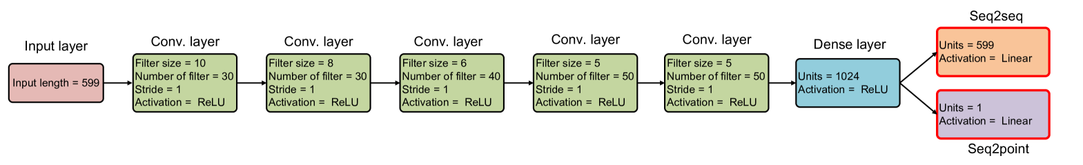
? [?] showed that denoising autoencoders performed better than other architectures for seq2seq learning. Instead, we propose to employ the same convolutional neural network for seq2seq and seq2point learning in this paper, as we will show in the following section that both approaches can have the same architecture, shown in Figure 1. ? [?] generated the training data heuristically. In contrast, we use all the sliding windows for both methods for training, thus not requiring heuristic rules for generating training data.

Table 1: The parameters used in this paper for each appliance. Power unit is Watt.

	Kettle	Microwave	Fridge	Dish Washer	Washing Machine
Window length (point)	599	599	599	599	599
Maximum power	3948	3138	2572	3230	3962
On power threshold	2000	200	50	10	20
Mean on power	700	500	200	700	400
Standard deviation on power	1000	800	400	1000	700

Posterior distribution estimators

In this section we show that both seq2seq and seq2point learning are essentially posterior density estimators. Suppose $T\rightarrow\infty$ , then we could have infinite number of sliding windows. They inherently form a population distribution $\pi(X|Y)$ which is unobserved, where $X$ and $Y$ are random temporally-aligned vectors of length $W$ . Seq2seq tries to find $\theta$ to maximise $p(X|Y,\theta)$ to approximate the population posterior $\pi(X|Y)$ . This could be achieved by minimizing Kullback-Leibler (KL) divergence with respect to $\theta$

\min_{\theta}KL(\pi||p)=\min_{\theta}\int\pi(X|Y)\log{\frac{\pi(X|Y)}{p(X|Y,\theta)}}dX.

So we have the standard interpretation that both methods are minimizing a Monte Carlo approximation to KL-divergence.

Now we will characterize the difference between seq2seq and seq2point learning. If we assume a factorizable form such that $p(X|Y,\theta)=\prod_{w=1}^{W}p_{w}(x_{w}|Y,\theta)$ , the objective function can then be represented as

KL(\pi||p)=\sum_{w=1}^{W}KL(\pi(x_{w}|Y)||p_{w}(x_{w}|Y,\theta)).

Now denote $\phi_{w}(\theta|Y)=KL(\pi(x_{w}|Y)||p_{w}(x_{w}|Y,\theta))$ which is a function of $\theta$ given $Y$ .

Seq2seq learning assumes the following distribution

	$\displaystyle p(X\|Y,\theta)$	$\displaystyle=\mathcal{N}(\mu(\theta),cI)=\prod_{w=1}^{W}\mathcal{N}(\mu_{w}(\theta),c)$
		$\displaystyle=\prod_{w=1}^{W}p_{w}(x_{w}\|Y,\theta)$

where $\mu(\theta)=(\mu_{1}(\theta),\cdots,\mu_{W}(\theta))^{T}$ , $c$ is a constant, and $I$ is the identity matrix. All the distributions $p_{w}$ partially share the same parameters $\theta$ except the parameters from the last hidden layer to outputs, and therefore, optimization needs to be performed jointly over all the distributions $p_{w}$ ( $w=1,2,\cdots,W$ ) such that

\min_{\theta}\sum_{w=1}^{W}\phi_{w}(\theta|Y).

Denote $\widetilde{\theta}$ as the optimum, the approximate distribution of the midpoint value is then $p_{\tau}(x_{\tau}|Y,\widetilde{\theta})$ by using seq2seq, and the corresponding KL-divergence for the midpoint value is $\phi_{\tau}(\widetilde{\theta}|Y)=KL(\pi(x_{\tau}|Y)||p_{\tau}(x_{\tau}|Y,\widetilde{\theta}))$ .

The seq2point learning directly models the midpoint value, and therefore, the optimization over $p(x_{\tau}|Y,\theta)$ can be performed by the following problem

\min_{\theta}\phi_{\tau}(\theta|Y).

Denote $\theta^{*}$ as the optimum, the approximate distribution of the midpoint value is then $p_{\tau}(x_{\tau}|Y,{\theta}^{*})$ . This shows that seq2seq and seq2point infer two different approximate distributions respectively to the same posterior distribution for midpoint value.

The following theorem shows that seq2point learning infers a tighter approximation to the target distribution than the seq2seq learning when they use the same architecture.

Theorem 1.

Assume all the distributions are well-defined. Suppose both the seq2point and seq2seq learning have the same architecture. Suppose $\theta^{*}$ is the optimum of the seq2point model, and $\widetilde{\theta}$ is the optimum of the seq2seq model. Then $\phi_{\tau}(\theta^{*}|Y)\leq\phi_{\tau}(\widetilde{\theta}|Y)$ .

Proof.

It is natural to assume that all the distributions are well-defined, and thus KL-divergence has a lower bound $0$ such that $\phi_{w}\geq 0$ . Since both learning methods have the same architecture, the functions $\phi_{w}$ for the two methods are the same. Since $\theta^{*}$ is the optimum of the problem $\min_{\theta}\phi_{\tau}(\theta|Y)$ , for any $\theta$ , $\phi_{\tau}(\theta^{*}|Y)\leq\phi_{\tau}(\theta|Y)$ . So $\phi_{\tau}(\theta^{*}|Y)+\sum_{w=1,w\neq\tau}^{W}\phi_{w}(\theta|Y)\leq\sum_{w=1}^{W}\phi_{w}(\theta|Y)$ is true for any $\theta$ . Therefore, $\phi_{\tau}(\theta^{*}|Y)+\sum_{w=1,w\neq\tau}^{W}\phi_{w}(\widetilde{\theta}|Y)\leq\sum_{w=1}^{W}\phi_{w}(\widetilde{\theta}|Y)$ . Consequently, $\phi_{\tau}(\theta^{*}|Y)\leq\phi_{\tau}(\widetilde{\theta}|Y)$ . ∎

This theorem ensures that seq2point learning always provides a tighter approximation than seq2seq learning.

Table 2: The appliance-level mean absolute error (MAE) (Watt) and signal aggregate error (SAE) for UK-DALE data. Best results are shown in bold. Seq2seq(Kelly) is proposed in (?).

Error measures	Methods	Kettle	Microwave	Fridge	Dish w.	Washing m.	Overall
MAE	AFHMM	47.38	21.18	42.35	199.84	103.24	82.79 $\pm$ 64.50
	seq2seq(Kelly)	13.000	14.559	38.451	237.96	163.468	93.488 $\pm$ 91.112
	seq2seq(this paper)	9.220	13.619	24.489	32.515	10.153	17.999 $\pm$ 9.063
	seq2point(this paper)	7.439	8.661	20.894	27.704	12.663	$\mathbf{15.472\pm 7.718}$
SAE	AFHMM	1.06	1.04	0.98	4.50	8.28	3.17 $\pm$ 2.88
	seq2seq(Kelly)	0.085	1.348	0.502	4.237	13.831	4.001 $\pm$ 5.124
	seq2seq(this paper)	0.309	0.205	0.373	0.779	0.453	0.423 $\pm$ 0.194
	seq2point(this paper)	0.069	0.486	0.121	0.645	0.284	$\mathbf{0.321\pm 0.217}$

Table 3: The appliance-level mean absolute error (MAE) (Watt) and signal aggregate error (SAE) for REDD data. Best results are shown in bold.

Error measures	Methods	Microwave	Fridge	Dish w.	Washing m.	Overall
MAE	seq2seq(this paper)	33.272	30.630	19.449	22.857	26.552 $\pm$ 5.610
MAE	seq2point(this paper)	28.199	28.104	20.048	18.423	$\mathbf{23.693\pm 4.494}$
SAE	seq2seq(this paper)	0.242	0.114	0.557	0.509	0.355 $\pm$ 0.183
SAE	seq2point(this paper)	0.059	0.180	0.567	0.277	$\mathbf{0.270\pm 0.187}$

Experiments

We compare four different models for the energy disaggregation problem, namely, the AFHMM (?), seq2seq(Kelly) (?), seq2seq, and seq2point. Note that seq2seq and seq2point use the same architecture (see Figure 1). There are two differences between the seq2seq proposed in this paper and the seq2seq(Kelly): 1) seq2seq uses the same training samples as seq2point where the samples were obtained by sliding the windows across all the data sequences; seq2seq(Kelly) uses selected windows obtained from all the data sequences, including some generated via data augmentation; 2) seq2seq uses a multilayer CNN architecture; seq2seq(Kelly) uses an autoencoder which includes a convolutional layer at each end. To verify the effectiveness and efficiency, we conduct comprehensive comparisons in terms of different performance metrics. The deep learning models are implemented in Python using TensorFlow. The networks were trained on machines with NVIDIA GTX 970 and NVIDIA GTX TITAN X GPUs.

Data sets

We report results on the UK-DALE (?) and REDD (?) data sets, which measured the domestic appliance-level energy consumption and whole-house energy usage of five UK houses and six US houses respectively.

UK-DALE data

All the readings were recorded in every 6 seconds from November 2012 to January 2015. The dataset contains the measurements of over 10 types of appliances, however, in this paper we are only interested in kettle, microwave, fridge, dish washer and washing machine which are popular appliances for evaluating NILM algorithms. We used the houses 1, 3, 4, and 5 for training the neural networks, and house 2 as the test data, because only houses 1 and 2 have all these appliances (?; ?). Note that we are therefore considering the transfer learning setting in which we train and test on different households. This setting has the challenge that the same type of appliance will vary in its power demands in different houses, but good performance in the transfer learning set-up is vital to practical application of NILM methods.

REDD data

The appliance and mains readings were recorded in every 3 seconds and 1 second respectively. The data set contains measurements from six houses. We used houses 2 to 6 for training, and house 1 for testing the algorithms, for similar reasons to those in ? [?]. Since there is no kettle data, we only looked at microwave, fridge, dish washer and washing machine.

Data preprocessing

We describe how the training data were prepared for training the neural networks. A window of the mains was used as the input sequence; the window length for each appliance is shown in the Table 1. The training windows were obtained by sliding the mains (input) and appliance (output) readings one timestep at a time; for seq2point, the midpoint values of the corresponding appliance windows were used as the outputs. Both the input windows and targets were preprocessed by subtracting the mean values and dividing by the standard deviations (see these parameters in the Table 1). These data samples were used for training both the seq2seq and seq2point methods. The training samples for training seq2seq(Kelly) were obtained by the method described in ? [?].

Performance evaluation

We use two metrics to compare these approaches. Denote $x_{t}$ as the ground truth and $\hat{x}_{t}$ the prediction of an appliance at time $t$ . When we are interested in the error in power at every time point, we use the mean absolute error (MAE)

\displaystyle\mbox{MAE}=\frac{1}{T}\sum_{t=1}^{T}|\hat{x}_{t}-x_{t}|.

This provides a measure of errors that is less affected by outliers, i.e. isolated predictions that are particularly inaccurate. When we are interested in the total error in energy over a period, in this case, one day, we use the normalised signal aggregate error (SAE)

\begin{aligned} \mbox{SAE}=\frac{|\hat{r}-r|}{r}\end{aligned},

where $r$ and $\hat{r}$ denote the ground truth and inferred total energy consumption of an appliance, that is $r=\sum_{t}x_{t}$ and $\hat{r}=\sum_{t}\hat{x}_{t}.$ This measure is useful because a method could be accurate enough for reports of daily power usage even if its per-timestep prediction is less accurate.

Experimental results

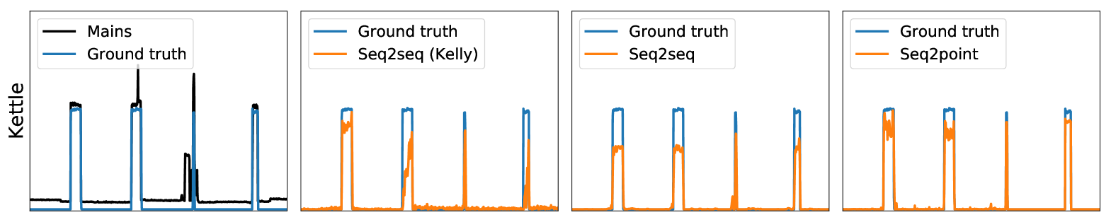
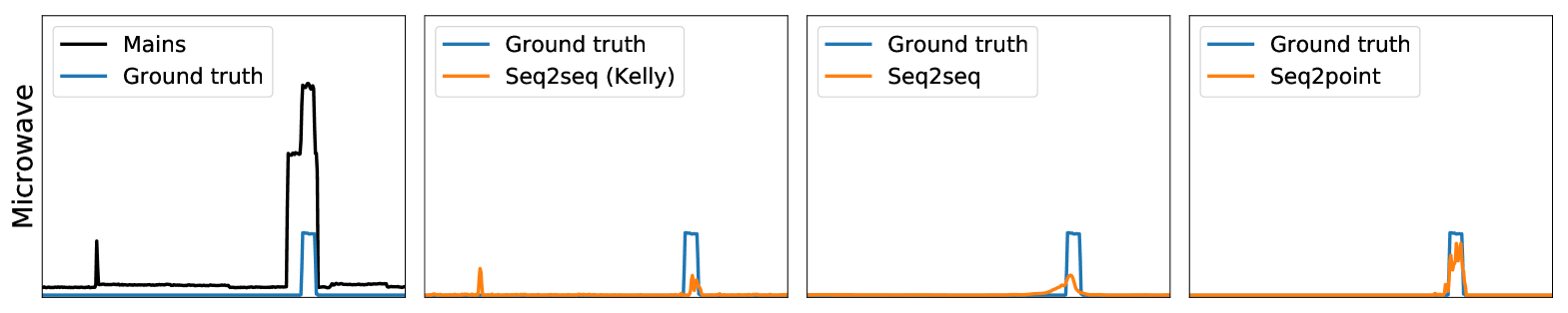
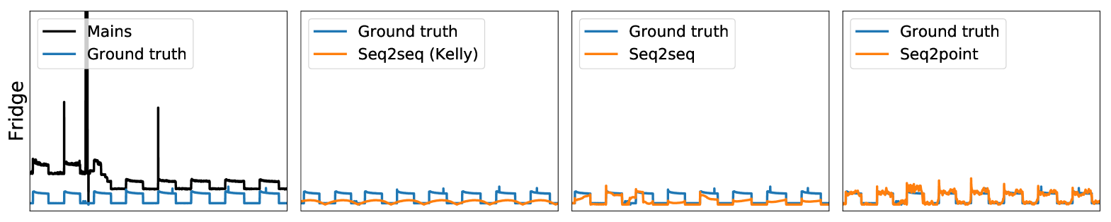
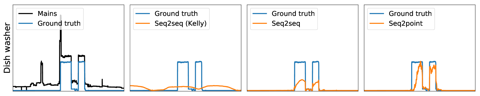
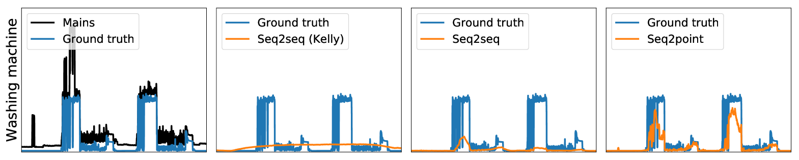
First, on the UK-DALE data, Table 2 shows that both the seq2seq and seq2point methods proposed in the paper outperformed the other two methods (AFHMM and seq2seq(Kelly). Our seq2seq reduces MAE by 81% and SAE by 89% overall compared to seq2seq(Kelly), with improvements in MAE for every appliance — this can be explained by our use of deeper architectures. Our seq2point method outperformed our seq2seq method in three out of four appliances, and overall — matching the results we obtained in the theorem. Compared to seq2seq(Kelly) our seq2point reduces MAE by 84% and SAE by 92%. We show example disaggregations on this data set performed by the three neural network methods in Figure 2.

Since AFHMM and seq2seq(Kelly) perform worse than our two methods on UK-DALE, we only applied our seq2seq and seq2point method to the REDD data set. The results are shown in Table 3. We can see that seq2point outperformed seq2seq in most of the appliances, and overall seq2point performs better than seq2seq — improving MAE by 11% and SAE by 24%, very close to the overall improvements on UK-DALE.

Visualization of latent features

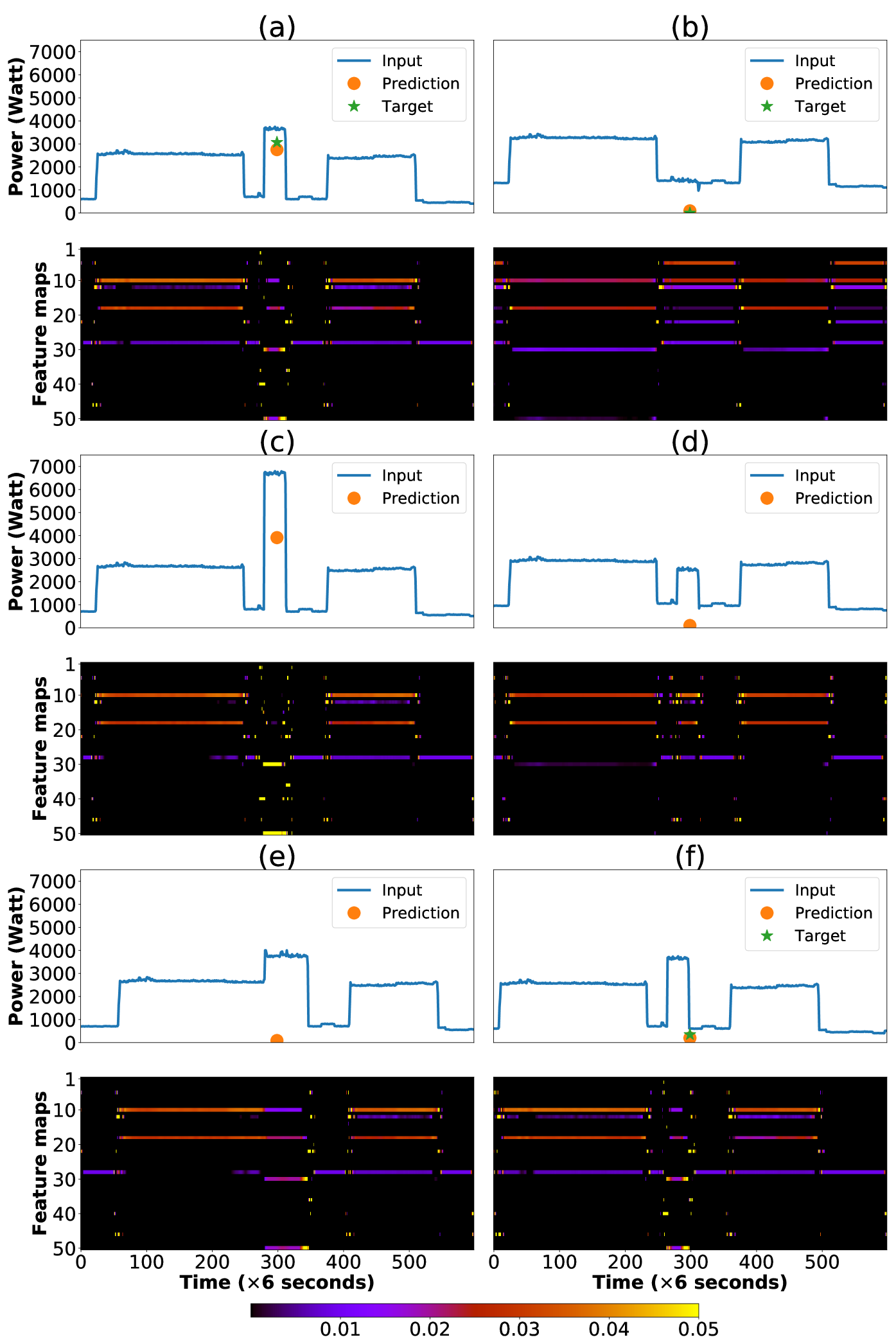
To validate the models, we would like to understand the reasons behind the network’s predictions. We expect that appliance signals have characteristic signatures that indicate when they are on. For example, a kettle only has two states: ON and OFF, and when it is ON the power should be approximately $2,000-3,000$ Watts; 2) the approximate duration of the kettle when it is ON. This information could be enough to detect a kettle. This information can greatly improve the performance of some algorithms (?; ?; ?).

Interestingly, we observed that the convolutional neural networks proposed in this paper are inherently learning these signatures. To test what the network has learnt, we take a window from the data, and manually modify it in ways that we believe should affect the prediction of the network. In these experiments we looked at the kettle which is easier to study because there are less number of states. For each different input, we plotted the feature maps of the last CNN layer in the Figure 3. It is interesting that all the filters detected the state changes of the appliances. More specifically, some filters take the responsibility of detecting amplitude of the appliance and as well as the state changes, but others only detect the state changes. Figure 3 (b) shows that when the kettle was manually removed, the network suggests that the amplitude of the signal and as well as the duration were not appropriate for a kettle. Figure 3 (c) shows that when the amplitude of the kettle was double, the network detects the kettle which is reasonable because both the duration and amplitude correspond to a kettle. Figure 3 (d) indicates that when the amplitude of the kettle was manually reduced, the network suggests there was no kettle. Figure 3 (e) shows that when the duration of the appliance usage was set too long ( $>8$ minutes), the network might suggest it was too long for a kettle. Figure 3 (f) shows that when there is no activation at the midpoint, the learnt signatures have the similar types to those in (a).

Conclusions

We have proposed a sequence-to-point learning with neural networks for energy disaggregation. We have applied the proposed schemes to real world data sets. We have shown that sequence-to-point learning outperforms previous work using sequence-to-sequence learning. By visualizing the learnt feature maps, we have shown that the neural networks learn meaningful features from the data, which are crucial signatures for performing energy disaggregation. It would be interesting to apply the proposed methods to the single-channel blind source separation problems in other domains, for example, audio and speech.

References

[Batra, Singh, and Whitehouse 2016] Batra, N.; Singh, A.; and Whitehouse, K. 2016. Gemello: Creating a detailed energy breakdown from just the monthly electricity bill. In Proceedings of the 22nd ACM SIGKDD International Conference on Knowledge Discovery and Data Mining, 431–440. ACM.
[Du et al. 2016] Du, J.; Tu, Y.; Dai, L.-R.; and Lee, C.-H. 2016. A regression approach to single-channel speech separation via high-resolution deep neural networks. IEEE/ACM Trans. Audio, Speech and Lang. Proc. 24(8):1424–1437.
[Fischer 2008] Fischer, C. 2008. Feedback on household electricity consumption: a tool for saving energy? Energy efficiency 1(1):79–104.
[Grais, Sen, and Erdogan 2014] Grais, E. M.; Sen, M. U.; and Erdogan, H. 2014. Deep neural networks for single channel source separation. In 2014 IEEE International Conference on Acoustics, Speech and Signal Processing (ICASSP), 3734–3738. IEEE.
[Hart 1992] Hart, G. 1992. Nonintrusive appliance load monitoring. Proceedings of the IEEE 80(12):1870 –1891.
[Huang et al. 2014] Huang, P.-S.; Kim, M.; Hasegawa-Johnson, M.; and Smaragdis, P. 2014. Deep learning for monaural speech separation. In 2014 IEEE International Conference on Acoustics, Speech and Signal Processing (ICASSP), 1562–1566. IEEE.
[Kelly and Knottenbelt 2015a] Kelly, J., and Knottenbelt, W. 2015a. Neural NILM: Deep neural networks applied to energy disaggregation. In Proceedings of the 2nd ACM International Conference on Embedded Systems for Energy-Efficient Built Environments, 55–64. ACM.
[Kelly and Knottenbelt 2015b] Kelly, J., and Knottenbelt, W. 2015b. The UK-DALE dataset, domestic appliance-level electricity demand and whole-house demand from five UK homes. Scientific Data 2(150007).
[Kolter and Jaakkola 2012] Kolter, Z., and Jaakkola, T. S. 2012. Approximate inference in additive factorial hmms with application to energy disaggregation. In AISTATS, volume 22, 1472–1482.
[Kolter and Johnson 2011] Kolter, J. Z., and Johnson, M. J. 2011. Redd: A public data set for energy disaggregation research.
[Lange and Bergés 2016] Lange, H., and Bergés, M. 2016. Efficient inference in dual-emission FHMM for energy disaggregation. In Workshops at the Thirtieth AAAI Conference on Artificial Intelligence.
[Parson et al. 2012] Parson, O.; Ghosh, S.; Weal, M.; and Rogers, A. 2012. Non-intrusive load monitoring using prior models of general appliance types. In Proceedings of the Twenty-Sixth Conference on Artificial Intelligence (AAAI-12), 356–362.
[Pattem 2012] Pattem, S. 2012. Unsupervised disaggregation for non-intrusive load monitoring. In Machine Learning and Applications (ICMLA), 2012 11th International Conference on, volume 2, 515–520. IEEE.
[Sainath et al. 2015] Sainath, T. N.; Kingsbury, B.; Saon, G.; Soltau, H.; rahman Mohamed, A.; Dahl, G.; and Ramabhadran, B. 2015. Deep convolutional neural networks for large-scale speech tasks. Neural Networks 64:39 – 48.
[Shaloudegi et al. 2016] Shaloudegi, K.; György, A.; Szepesvari, C.; and Xu, W. 2016. SDP relaxation with randomized rounding for energy disaggregation. In Lee, D. D.; Sugiyama, M.; Luxburg, U. V.; Guyon, I.; and Garnett, R., eds., Advances in Neural Information Processing Systems 29. Curran Associates, Inc. 4979–4987.
[Sutskever, Vinyals, and Le 2014] Sutskever, I.; Vinyals, O.; and Le, Q. 2014. Sequence to sequence learning with neural networks. In Advances in Neural Information Processing Systems (NIPS).
[Tabatabaei, Dick, and Xu 2017] Tabatabaei, S. M.; Dick, S.; and Xu, W. 2017. Toward non-intrusive load monitoring via multi-label classification. IEEE Transactions on Smart Grid 8(1):26–40.
[van den Oord et al. 2016] van den Oord, A.; Dieleman, S.; Zen, H.; Simonyan, K.; Vinyals, O.; Graves, A.; Kalchbrenner, N.; Senior, A.; and Kavukcuoglu, K. 2016. Wavenet: A generative model for raw audio. arXiv preprint arXiv:1609.03499.
[van den Oord, Kalchbrenner, and Kavukcuoglu 2016] van den Oord, A.; Kalchbrenner, N.; and Kavukcuoglu, K. 2016. Pixel recurrent neural networks. In Proceedings of The 33rd International Conference on Machine Learning, 1747–1756.
[Zhao, Stankovic, and Stankovic 2015] Zhao, B.; Stankovic, L.; and Stankovic, V. 2015. Blind non-intrusive appliance load monitoring using graph-based signal processing. In 2015 IEEE Global Conference on Signal and Information Processing (GlobalSIP), 68–72.
[Zhao, Stankovic, and Stankovic 2016] Zhao, B.; Stankovic, L.; and Stankovic, V. 2016. On a training-less solution for non-intrusive appliance load monitoring using graph signal processing. IEEE Access 4:1784–1799.
[Zhong, Goddard, and Sutton 2013] Zhong, M.; Goddard, N.; and Sutton, C. 2013. Interleaved factorial non-homogeneous hidden Markov models for energy disaggregation. In Neural Information Processing Systems, Workshop on Machine Learning for Sustainability.
[Zhong, Goddard, and Sutton 2014] Zhong, M.; Goddard, N.; and Sutton, C. 2014. Signal aggregate constraints in additive factorial HMMs, with application to energy disaggregation. In Advances in Neural Information Processing Systems, 3590–3598.
[Zhong, Goddard, and Sutton 2015] Zhong, M.; Goddard, N.; and Sutton, C. 2015. Latent Bayesian melding for integrating individual and population models. In Advances in Neural Information Processing Systems, 3618–3626.