This paper was converted on www.awesomepapers.org from LaTeX by an anonymous user.
Want to know more? Visit the Converter page.

Sequential Monte Carlo algorithms for agent-based models of disease transmission

Nianqiao Ju Corresponding author: nju@g.harvard.edu Department of Statistics, Harvard University, USA Jeremy Heng ESSEC Business School, Singapore Pierre E. Jacob Department of Statistics, Harvard University, USA
Abstract

Agent-based models of disease transmission involve stochastic rules that specify how a number of individuals would infect one another, recover or be removed from the population. Common yet stringent assumptions stipulate interchangeability of agents and that all pairwise contact are equally likely. Under these assumptions, the population can be summarized by counting the number of susceptible and infected individuals, which greatly facilitates statistical inference. We consider the task of inference without such simplifying assumptions, in which case, the population cannot be summarized by low-dimensional counts. We design improved particle filters, where each particle corresponds to a specific configuration of the population of agents, that take either the next or all future observations into account when proposing population configurations. Using simulated data sets, we illustrate that orders of magnitude improvements are possible over bootstrap particle filters. We also provide theoretical support for the approximations employed to make the algorithms practical.

1 Introduction

1.1 Statistical inference for agent-based models

Agent-based models also called individual-based models are used in many fields, such as social sciences (Epstein, 2006), demographics (Hooten et al., 2020), ecology (DeAngelis and Gross, 2018) and macroeconomics (Turrell, 2016). These models describe the time evolution of a population according to a Markov process. The population comprises of NN\in\mathbb{N} agents who interact with one another through a probabilistic mechanism. The popularity of these models could be attributed to the ease of model building and interpretation, while allowing the representation of complex phenomena. Specialized software is available to facilitate their simulation and the visualization of their output (e.g. Tisue and Wilensky, 2004).

The primary use of these models seems to involve “forward simulations” using various parameters corresponding to hypothetical scenarios. In comparison, relatively fewer works have tackled the question of statistical inference for such models, i.e. the estimation of model parameters given available observations, also known as model calibration. Broad articles on the question of fitting agent-based models include Grazzini et al. (2017); Hooten et al. (2020); Hazelbag et al. (2020) and this is a very active research area. The question of estimation is well-posed: by viewing agent-based models as a subclass of hidden Markov models, we can define the associated likelihood function, from which maximum likelihood and Bayesian procedures can be envisioned.

Gibbs sampling or “data augmentation” Markov chain Monte Carlo (MCMC) methods, that alternate between parameter and latent agent states updates are generically applicable, see Fintzi et al. (2017); Bu et al. (2020) in the context of disease transmission. However, the mixing properties of these chains can be problematic, as we illustrate in Appendix C. Likelihood-based inference that avoid the use of data augmentation requires one to marginalize out the latent population process. This is computationally challenging as the number of possible configurations of the population of agents grows exponentially in NN. Our contribution is to design improved particle filters to estimate the likelihood function of agent-based models, which can then be used for parameter inference procedures such as simulated maximum likelihood and particle MCMC (Andrieu et al., 2010). Particle MCMC methods, based on more standard particle filters, have been used for agent-based models before, see e.g. Kattwinkel and Reichert (2017). For indirect inference and approximate Bayesian computation applied to agent-based models we refer to (Platt, 2020; van der Vaart et al., 2016; Chen et al., 2017; Sirén et al., 2018).

1.2 Statistical inference for agent-based models of disease transmission

We limit the scope of this article to some agent-based models of disease transmission. We next introduce a specific model which will be used to draw clear connections between agent-based models and more tractable but restrictive formulations of disease outbreak models.

The state of agent nn at time tt, denoted by XtnX_{t}^{n}, takes the value 0 or 11, corresponding to a “susceptible” or “infected” status in the context of disease transmission. We consider a closed population of size NN, TT\in\mathbb{N} time steps and a stepsize of h>0h>0. Initial agent states follow independent Bernoulli distributions, i.e.

X0nBer(α0),X_{0}^{n}\sim\text{Ber}(\alpha_{0}), (1)

for n[1:N]={1,,N}n\in[1:N]=\{1,\ldots,N\}, where we assume for the time being that each agent has the same probability α0(0,1)\alpha_{0}\in(0,1) of being infected. The state of the population Xt=(Xtn)n[1:N]{0,1}NX_{t}=(X_{t}^{n})_{n\in[1:N]}\in\{0,1\}^{N} evolves according to a Markov process that depends on the interactions between the agents. The Markov transition specifies that, given the previous states xth{0,1}Nx_{t-h}\in\{0,1\}^{N}, the next agent states (Xtn)n[1:N](X_{t}^{n})_{n\in[1:N]} are conditionally independent Bernoulli variables with probabilities (αn(xth))n[1:N](\alpha^{n}(x_{t-h}))_{n\in[1:N]} given by

αn(xth)={hλN1m=1Nxthm,if xthn=0,1hγ,if xthn=1.\displaystyle\alpha^{n}(x_{t-h})=\begin{cases}h\lambda N^{-1}\sum_{m=1}^{N}x_{t-h}^{m},\quad&\mbox{if }x_{t-h}^{n}=0,\\ 1-h\gamma,\quad&\mbox{if }x_{t-h}^{n}=1.\end{cases} (2)

Here λ(0,1)\lambda\in(0,1) and γ(0,1)\gamma\in(0,1) represent infection and recovery rate parameters respectively. An uninfected agent becomes infected with probability proportional to λ\lambda and to the proportion of infected individuals. An infected agent recovers with probability proportional to γ\gamma. The ratio R0=λ/γR_{0}=\lambda/\gamma is known as the basic reproductive number, which characterizes the transmission potential of a disease (Lipsitch et al., 2003; Britton, 2010). The latent population process (Xt)(X_{t}) can be related to aggregated observations (Yt)(Y_{t}) of the entire population. For example, the number of infections reported at each time could be modelled as a Binomial distribution, i.e.

YtXt=xtBin(I(xt),ρ),Y_{t}\mid X_{t}=x_{t}\sim\text{Bin}(I(x_{t}),\rho), (3)

where I(xt)=n=1Nxtn[0:N]I(x_{t})=\sum_{n=1}^{N}x_{t}^{n}\in[0:N] counts the number of infected individuals and ρ(0,1)\rho\in(0,1) represents a reporting rate. Equations (1), (2) and (3) define a susceptible-infected-susceptible (SIS) hidden Markov model.

As the latent state space has cardinality 2N2^{N}, evaluating the likelihood function with the forward algorithm would be impractical. Statistical inference is still feasible as the latent process admits low-dimensional summaries. Since (2) assumes that all agents are interchangeable and all pairwise contact are equally likely, the dynamics depends only on the number of infected individuals It=I(Xt)I_{t}=I(X_{t}) and susceptible individuals St=NItS_{t}=N-I_{t}. More precisely, the Markov transition for each t>0t>0 can be summarized as

St=Sth+NtSNtI,It=IthNtS+NtI,\displaystyle S_{t}=S_{t-h}+N^{S}_{t}-N^{I}_{t},\qquad I_{t}=I_{t-h}-N^{S}_{t}+N^{I}_{t}, (4)

where NtSBin(Ith,hγ)N^{S}_{t}\sim\text{Bin}(I_{t-h},h\gamma) and NtIBin(Sth,hλN1Ith)N^{I}_{t}\sim\text{Bin}(S_{t-h},h\lambda N^{-1}I_{t-h}) denote the number of new recoveries and infections, respectively. The initialization in (1) corresponds to having I0Bin(N,α0)I_{0}\sim\text{Bin}(N,\alpha_{0}) and S0=NI0S_{0}=N-I_{0}. The process (St,It)(S_{t},I_{t}) is a Markov chain on the lower-dimensional state space {n,m[0:N]:n+m=N}\{n,m\in[0:N]:n+m=N\}, and not in {0,1}N\{0,1\}^{N}. When combined with (3), the resulting hidden Markov model can be estimated using particle filtering strategies; see e.g. Ionides et al. (2006); Endo et al. (2019); Whiteley and Rimella (2020).

For large population sizes NN, one can exploit the asymptotic properties of the dynamics (4) to further simplify inference procedures. As NN\rightarrow\infty, the finite population proportions S¯tN=St/N\bar{S}_{t}^{N}=S_{t}/N and I¯tN=It/N\bar{I}_{t}^{N}=I_{t}/N admit deterministic limits S¯t\bar{S}_{t} and I¯t\bar{I}_{t}, defined by the recursion

S¯t=S¯th+hγI¯thλS¯tI¯t,I¯t=I¯thhγI¯t+hλS¯tI¯t,\displaystyle\bar{S}_{t}=\bar{S}_{t-h}+h\gamma\bar{I}_{t}-h\lambda\bar{S}_{t}\bar{I}_{t},\qquad\bar{I}_{t}=\bar{I}_{t-h}-h\gamma\bar{I}_{t}+h\lambda\bar{S}_{t}\bar{I}_{t}, (5)

with initial condition (S¯t,I¯t)=(1α0,α0)(\bar{S}_{t},\bar{I}_{t})=(1-\alpha_{0},\alpha_{0}). If fine time resolutions are desired, one can also consider the limit h0h\rightarrow 0, in which case (S¯t,I¯t)(\bar{S}_{t},\bar{I}_{t}) converges to a deterministic continuous-time process (S¯(t),I¯(t))(\bar{S}(t),\bar{I}(t)), defined by the following system of ordinary differential equations

dS¯(t)dt=γI¯(t)λS¯(t)I¯(t),dI¯(t)dt=γI¯(t)+λS¯(t)I¯(t),\displaystyle\frac{d\bar{S}(t)}{dt}=\gamma\bar{I}(t)-\lambda\bar{S}(t)\bar{I}(t),\qquad\frac{d\bar{I}(t)}{dt}=-\gamma\bar{I}(t)+\lambda\bar{S}(t)\bar{I}(t), (6)

with (S¯(0),I¯(0))=(1α0,α0)(\bar{S}(0),\bar{I}(0))=(1-\alpha_{0},\alpha_{0}). We refer to Allen and Burgin (2000) and Allen et al. (2008, Chapter 3) for formal links between stochastic and deterministic SIS models, in the form of limit theorems as NN\to\infty. The dynamics in (5) or (6) combined with an observation model such as (3) leads again to a fairly tractable statistical model, which can be estimated by maximum likelihood or in the Bayesian framework (e.g. Osthus et al., 2019).

The tractability in (4) and its limits (5)-(6) hinges critically on the assumption that all agents are interchangeable and equally likely to be in contact. These assumptions are strong as it would be desirable to let the infection and recovery rates depend on individual characteristics or features, and the structure of interactions be specified by an undirected network. Adopting any one of these generalizations would result in an agent-based model that cannot be summarized by low-dimensional counts. This article is concerned with the task of inference when these assumptions are relaxed. Our approach is to return to the hidden Markov model formulation with latent space {0,1}N\{0,1\}^{N}, and seek novel sampling algorithms that have polynomial rather than exponential costs in NN. The guiding principle of our contribution is that we can improve the performance of Monte Carlo algorithms, sometimes dramatically, by tailoring them to the models at hand, and by using available observations.

The rest of this article is organized as follows. In Section 2, we consider a “static” case with a single time step to illustrate some of the challenges and proposed solutions in a simple setting. We describe how the cost of likelihood evaluation and sampling the posterior of agent states given observations can be reduced from exponential to polynomial in NN. In Section 3, we consider the dynamic setting with multiple time steps and design auxiliary particle filters and controlled SMC algorithms tailored to heterogeneous SIS agent-based models. We also provide theoretical support for the approximations employed to make the algorithms practical. We extend our methodology to susceptible-infected-recovered (SIR) models in Section 4 and highlight the associated difficulties. Section 5 summarizes our findings and open questions. This manuscript represents preliminary work and further numerical experiments will be added in a later version. The code is available at https://github.com/nianqiaoju/agents. The proofs and more details are in appendices.

2 Static agent-based model

For simplicity we begin with the static model XnBer(αn)X^{n}\sim\text{Ber}(\alpha^{n}) independently for n[1:N]n\in[1:N], and allow each agent to be unique by modeling αn=(1+exp(βwn))1\alpha^{n}=(1+\exp(-\beta^{\top}w^{n}))^{-1}, where βd\beta\in\mathbb{R}^{d} are parameters and wndw^{n}\in\mathbb{R}^{d} are the covariates of agent nn. This allows individual factors to account for the probability of infection α=(αn)n[1:N]\alpha=(\alpha^{n})_{n\in[1:N]}. Given an observation y[0:N]y\in[0:N] modelled as (3), our inferential objective might include estimating the unknown parameters θ=(β,ρ)Θ\theta=(\beta,\rho)\in\Theta and/or the latent states X=(Xn)n[1:N]{0,1}NX=(X^{n})_{n\in[1:N]}\in\{0,1\}^{N}. The complete data likelihood is pθ(x,y)=fθ(x)gθ(y|x)p_{\theta}(x,y)=f_{\theta}(x)g_{\theta}(y|x), where

fθ(x)=n=1NBer(xn;αn),gθ(y|x)=Bin(y;I(x),ρ)𝟙(I(x)y).f_{\theta}(x)=\prod_{n=1}^{N}\text{Ber}(x^{n};\alpha^{n}),\quad g_{\theta}(y|x)=\text{Bin}(y;I(x),\rho)\mathbbm{1}(I(x)\geq y). (7)

Here Ber(xn;αn)\text{Ber}(x^{n};\alpha^{n}) and Bin(y;I(x),ρ)\text{Bin}(y;I(x),\rho) denote the corresponding probability mass functions (PMF). Marginalizing over the latent states yields the likelihood pθ(y)p_{\theta}(y). The agent states given the observation and a parameter follow the posterior distribution pθ(x|y)p_{\theta}(x|y). In Sections 2.1 and 2.2, we examine the cost of exactly computing pθ(y)p_{\theta}(y) and sampling from pθ(x|y)p_{\theta}(x|y), respectively, and describe cheaper approximations. The gains are assessed numerically in Section 2.3.

2.1 Marginal likelihood computations

A naive approach to compute the marginal likelihood pθ(y)p_{\theta}(y) is to sum over all possible population configurations

pθ(y)=x{0,1}Npθ(x,y)=x{0,1}Nfθ(x)gθ(y|x).p_{\theta}(y)=\sum_{x\in\{0,1\}^{N}}p_{\theta}(x,y)=\sum_{x\in\{0,1\}^{N}}f_{\theta}(x)g_{\theta}(y|x). (8)

This requires 𝒪(2N)\mathcal{O}(2^{N}) operations. A simple Monte Carlo approach involves sampling X(p)=(X(p),n)n[1:N]fθX^{(p)}=(X^{(p),n})_{n\in[1:N]}\sim f_{\theta} independently for p[1:P]p\in[1:P], which represents PP possible configurations of the population, and return the Monte Carlo estimator P1p=1Pgθ(y|X(p))P^{-1}\sum_{p=1}^{P}g_{\theta}(y|X^{(p)}) that weights each configuration according to the observation density. The estimator is unbiased and only costs 𝒪(NP)\mathcal{O}(NP) to compute, but its variance might be prohibitively large for practical values of PP, depending on the observation model gθ(y|x)g_{\theta}(y|x). Another issue with this estimator is that it can collapse to zero whenever I(X(p))<yI(X^{(p)})<y for all p[1:P]p\in[1:P]. Following Del Moral et al. (2015), this can be circumvented by repeatedly drawing samples X(p)fθX^{(p)}\sim f_{\theta} independently until there are PP configurations that satisfy I(X(p))yI(X^{(p)})\geq y, and return the estimator (R1)1p=1R1gθ(y|X(p)){(R-1)}^{-1}\sum_{p=1}^{R-1}g_{\theta}(y|X^{(p)}), where RPR\geq P denotes the number of repetitions needed. The resulting estimator can be shown to be unbiased and has a random cost of 𝒪(N𝔼[R])\mathcal{O}(N\,\mathbb{E}[R]), that depends on the value of yy. An obvious shortcoming of the above estimators is that the agents are sampled from fθf_{\theta} without using the available observation yy.

We can in fact reduce the cost of computing (8) without resorting to Monte Carlo approximations. The starting observation is that I=I(X)I=I(X) under XfθX\sim f_{\theta} is the sum of NN independent Bernoulli random variables with non-identical success probabilities, and follows a distribution called “Poisson Binomial”. We will refer to this distribution as PoiBin(α\alpha) and write its PMF as

PoiBin(i;α)=x{0,1}N𝟙(n=1Nxn=i)n=1N(αn)xn(1αn)(1xn),i[0:N].\text{PoiBin}(i;\alpha)=\sum_{x\in\{0,1\}^{N}}\mathbbm{1}\left(\sum_{n=1}^{N}x^{n}=i\right)\prod_{n=1}^{N}(\alpha^{n})^{x^{n}}(1-\alpha^{n})^{(1-x^{n})},\quad i\in[0:N]. (9)

Exact evaluation of (9) has been considered in Barlow and Heidtmann (1984); Chen et al. (1994); Chen and Liu (1997); Hong (2013) using different approaches. Defining q(i,n)=PoiBin(i;αn:N)q(i,n)=\text{PoiBin}(i;\alpha^{n:N}) for i[0:N]i\in[0:N] and n[1:N]n\in[1:N], we will employ the following recursion

q(i,n)=αnq(i1,n+1)+(1αn)q(i,n+1),i[1:N],n[1:N1],q(i,n)=\alpha^{n}q(i-1,n+1)+(1-\alpha^{n})q(i,n+1),\quad i\in[1:N],n\in[1:N-1], (10)

with initial conditions q(0,n)=m=nN(1αm)q(0,n)=\prod_{m=n}^{N}(1-\alpha^{m}) for n[1:N]n\in[1:N], q(1,N)=αNq(1,N)=\alpha^{N} and q(i,N)=0q(i,N)=0 for i[2:N]i\in[2:N]. The desired PMF q(i,1)=PoiBin(i;α)q(i,1)=\text{PoiBin}(i;\alpha) for i[0:N]i\in[0:N] can thus be computed in 𝒪(N2)\mathcal{O}(N^{2}) operations; see Appendix A.1 for a derivation of (10).

Using the above observation, we can rewrite the marginal likelihood as

pθ(y)=i=0NPoiBin(i;α)Bin(y;i,ρ)𝟙(iy),p_{\theta}(y)=\sum_{i=0}^{N}\text{PoiBin}(i;\alpha)\text{Bin}(y;i,\rho)\mathbbm{1}(i\geq y), (11)

which costs 𝒪(N2)\mathcal{O}(N^{2}) to compute. Using a thinning argument detailed in Appendix A.2, the above sum is in fact equal to pθ(y)=PoiBin(y;ρα)p_{\theta}(y)=\text{PoiBin}(y;\rho\,\alpha). Although the marginal likelihood will not admit such tractability in the general setup considered in Section 3, the preceding observations will guide our choice of approximations.

One can also rely on approximations of the Poisson Binomial distribution to further reduce the cost of computing (11) to 𝒪(N)\mathcal{O}(N). Choices include the Poisson approximation (Hodges and Le Cam, 1960; Barbour and Hall, 1984; Wang, 1993), the Normal approximation (Volkova, 1996) and the translated Poisson approximation (Barbour and Xia, 1999; Cekanavicius and Vaitkus, 2001; Barbour and Ćekanavićius, 2002). We will focus on the translated Poisson approximation which exactly matches the mean and approximately the variance of a Poisson Binomial distribution. Let Poi(λ)\text{Poi}(\lambda) denote a Poisson distribution with rate λ>0\lambda>0 and write the mean and variance of PoiBin(α\alpha) as μ=n=1Nαn\mu=\sum_{n=1}^{N}\alpha^{n} and σ2=n=1Nαn(1αn)\sigma^{2}=\sum_{n=1}^{N}\alpha^{n}(1-\alpha^{n}), respectively. The translated Poisson approximation of (9) is given by

TransPoi(i;μ,σ2)={0,i[0:μσ21],Poi(iμσ2;σ2+{μσ2}),i[μσ2:N],\text{TransPoi}(i;\mu,\sigma^{2})=\begin{cases}0,&i\in[0:\lfloor\mu-\sigma^{2}\rfloor-1],\\ \text{Poi}(i-\lfloor\mu-\sigma^{2}\rfloor;\sigma^{2}+\{\mu-\sigma^{2}\}),&i\in[\lfloor\mu-\sigma^{2}\rfloor:N],\end{cases} (12)

where μσ2\lfloor\mu-\sigma^{2}\rfloor and {μσ2}\{\mu-\sigma^{2}\} denote the floor and fractional part of μσ2\mu-\sigma^{2}, respectively. Since μ\mu and σ2\sigma^{2} can be computed in 𝒪(N)\mathcal{O}(N) operations, the translated Poisson approximation (12) and the resulting approximation of (11) only require 𝒪(N)\mathcal{O}(N) operations. Hence this can be appealing in the setting of large population sizes NN at the expense of an approximation error that is well-studied. Indeed results in Cekanavicius and Vaitkus (2001, Theorem 2.1 & Corollary 2.1) and Barbour and Ćekanavićius (2002, Theorem 3.1) imply that the error, measured in the total variation distance, decay at the rate of N1/2N^{-1/2} as NN\rightarrow\infty.

2.2 Posterior sampling of agent states

Sampling from the posterior distribution pθ(x|y)p_{\theta}(x|y) by naively enumerating over all 2N2^{N} configurations is computationally impractical. A key observation is that the observation density in (7) depends on the high dimensional latent state X{0,1}NX\in\{0,1\}^{N} only through the one-dimensional summary I(X)[0:N]I(X)\in[0:N]. This prompts the inclusion of I=I(X)I=I(X) as an auxiliary variable. Thus the joint posterior distribution can be decomposed as

pθ(x,i|y)=pθ(i|y)pθ(x|i).\displaystyle p_{\theta}(x,i|y)=p_{\theta}(i|y)p_{\theta}(x|i). (13)

The dominant cost of sampling the posterior distribution of the summary

pθ(i|y)=pθ(i)pθ(y|i)pθ(y)=PoiBin(i;α)Bin(y;i,ρ)𝟙(iy)pθ(y),i[0:N],\displaystyle p_{\theta}(i|y)=\frac{p_{\theta}(i)p_{\theta}(y|i)}{p_{\theta}(y)}=\frac{\text{PoiBin}(i;\alpha)\text{Bin}(y;i,\rho)\mathbbm{1}(i\geq y)}{p_{\theta}(y)},\quad i\in[0:N], (14)

is the evaluation of the Poisson Binomial PMF (9). Recall from Section 2.1 that this can be done exactly in 𝒪(N2)\mathcal{O}(N^{2}), and in 𝒪(N)\mathcal{O}(N) using a translated Poisson approximation. The conditional distribution of the latent state given the summary

pθ(x|i)=pθ(x)pθ(i|x)pθ(i)=n=1N(αn)xn(1αn)1xn𝟙(I(x)=i)PoiBin(i;α)\displaystyle p_{\theta}(x|i)=\frac{p_{\theta}(x)p_{\theta}(i|x)}{p_{\theta}(i)}=\frac{\prod_{n=1}^{N}(\alpha^{n})^{x^{n}}(1-\alpha^{n})^{1-x^{n}}\mathbbm{1}(I(x)=i)}{\text{PoiBin}(i;\alpha)} (15)

is known as a conditional Bernoulli distribution, which we will write as pθ(x|i)=CondBer(x;α,i)p_{\theta}(x|i)=\text{CondBer}(x;\alpha,i). Various sampling schemes have been proposed (Fan et al., 1962; Chen et al., 1994); see Chen and Liu (1997, Section 4) for an overview. We will rely on the sequential decomposition

pθ(x|i)\displaystyle p_{\theta}(x|i) =pθ(x1|i)n=2Npθ(xn|x1:n1,i)\displaystyle=p_{\theta}(x^{1}|i)\prod_{n=2}^{N}p_{\theta}(x^{n}|x^{1:n-1},i) (16)
=n=1N1(αn)xn(1αn)1xnq(iin1xn,n+1)q(iin1,n)𝟙(xN=iiN1),\displaystyle=\prod_{n=1}^{N-1}\frac{(\alpha^{n})^{x^{n}}(1-\alpha^{n})^{1-x^{n}}q(i-i_{n-1}-x^{n},n+1)}{q(i-i_{n-1},n)}\mathbbm{1}(x^{N}=i-i_{N-1}),

where i0=0i_{0}=0 and in=m=1nxmi_{n}=\sum_{m=1}^{n}x^{m} for n[1:N1]n\in[1:N-1]. A derivation of (16) can be found in Appendix A of Heng et al. (2020b). The values of q(j,n)q(j,n) for j[0:i],n[1:N]j\in[0:i],n\in[1:N] needed in (16) can be precomputed using the same recursion as (10) in 𝒪(iN)\mathcal{O}(iN) cost. This precomputation is not necessary if these values are stored when computing Poisson Binomial probabilities.

To reduce the cost we can employ a Markov chain Monte Carlo (MCMC) method to sample from the conditional Bernoulli distribution CondBer(α,i)\text{CondBer}(\alpha,i). This incurs a cost of 𝒪(1)\mathcal{O}(1) per iteration and converges in 𝒪(NlogN)\mathcal{O}(N\log N) iterations, under some mild assumptions on α\alpha, as shown in Heng et al. (2020b). On a related note, we can design MCMC algorithms to target pθ(x|y)p_{\theta}(x|y). These might for example update the state of a few agents by sampling from their conditional distributions given every other variables, and alternately propose to swap zeros and ones in the vector X{0,1}NX\in\{0,1\}^{N}. Each of these steps can be done with a cost independent of NN, but the number of iterations for the algorithm to converge is expected to grow at least linearly with NN.

2.3 Numerical illustration

We set up numerical experiments as follows. We generate covariates (wn)(w^{n}) from 𝒩(4,1)\mathcal{N}(4,1) for N=1000N=1000 individuals independently, where 𝒩(μ,σ2)\mathcal{N}(\mu,\sigma^{2}) denotes a Normal distribution with mean μ\mu\in\mathbb{R} and variance σ2>0\sigma^{2}>0. Individual specific infection probabilities are computed as αn=(1+exp(βwn))1\alpha^{n}=(1+\exp(-\beta w^{n}))^{-1} using β=0.3\beta=0.3. We then simulate XnBer(αn)X^{n}\sim\text{Ber}(\alpha^{n}) independently for all nn, and sample YBin(n=1NXn,ρ)Y\sim\text{Bin}(\sum_{n=1}^{N}X^{n},\rho), with ρ=0.8\rho=0.8. We adopt a Bayesian approach and assign an independent prior of 𝒩(0,1)\mathcal{N}(0,1) on β\beta and Uniform(0,1)\text{Uniform}(0,1) on ρ\rho. We focus on the task of sampling from the posterior distribution of θ=(β,ρ)\theta=(\beta,\rho) given yy and the covariates (wn)(w^{n}).

We consider random walk Metropolis–Hastings with exact likelihood calculation (“MH-exact”), associated with a quadratic cost in NN. We also consider the same algorithm with a likelihood approximated by a translated Poisson (“MH-tp”), with a cost linear in NN. Finally we consider a pseudo-marginal approach (Andrieu and Roberts, 2009; Andrieu et al., 2010) with likelihood estimated with P=20P=20 particles sampled from fθf_{\theta} (“PMMH”). Note that P=20P=20 samples resulted in a variance of the log-likelihood estimates of approximately 0.30.3 at the data generating parameters (DGP). These samplers employ the same random walk, based on Normal proposals, independently on β\beta and log(ρ/(1ρ))\log(\rho/(1-\rho)) with standard deviation of 0.20.2. As a baseline we also consider a Gibbs sampler that alternates between the updates of θ\theta given XX, employing the same proposal as above, and updates of XX given θ\theta. These employ an equally weighted mixture of kernels, performing either NN random swap updates, or a systematic Gibbs scan of the NN components of XX; thus the cost per iteration is linear in NN.

We first run “MH-exact” with 100,000100,000 MCMC iterations (after a burn-in of 5,0005,000 iterations), to obtain estimates of the posterior means of β\beta and ρ\rho. Using these posterior estimates as ground truth, we compute the mean squared error (MSE) of the posterior approximations obtained using each method with 20,00020,000 MCMC iterations (excluding a burn-in of 50005000) and 50 independent repetitions. Table 1 displays the MSE, as well as the relative wall-clock time to obtain each estimate. Comparing the results of MH-exact and MH-tp shows that it is possible to save considerable efforts at the expense of small differences in the parameter estimates using a translated Poisson approximation. The appeal of the PMMH approach compared to exact likelihood calculations is also clear. On the other hand, Gibbs samplers that alternate between the updates of θ\theta and XX do not seem to be competitive in this example.

Method 𝔼[β|y]\mathbb{E}[\beta|y] 𝔼[ρ|y]\mathbb{E}[\rho|y] Relative cost
Bias2 Variance Bias2 Variance
MH-exact 25 93.3 0.74 6.39 128
MH-tp 22 52.3 0.32 2.83 1
PMMH 18 79.2 0.50 4.67 8
Gibbs 1040 113 91.1 2.85 42
Table 1: Bias and variance when approximating the posterior mean of β\beta and ρ\rho with each inference method (in units of 10410^{-4}). The rightmost column displays the average cost for each method measured in terms of run-time, relative to MH-tp.

3 Susceptible-Infected-Susceptible model

We now extend the agent-based SIS model in Section 1.2. To allow for individual-specific attributes, for agent n[1:N]n\in[1:N], we model her initial infection probability α0n\alpha_{0}^{n}, infection rate λn\lambda^{n} and recovery rate γn\gamma^{n} as

α0n=(1+exp(β0wn))1,λn=(1+exp(βλwn))1,γn=(1+exp(βγwn))1.\displaystyle\alpha_{0}^{n}=(1+\exp(-\beta_{0}^{\top}w^{n}))^{-1},\quad\lambda^{n}=(1+\exp(-\beta_{\lambda}^{\top}w^{n}))^{-1},\quad\gamma^{n}=(1+\exp(-\beta_{\gamma}^{\top}w^{n}))^{-1}. (17)

Here β0,βλ,βγd\beta_{0},\beta_{\lambda},\beta_{\gamma}\in\mathbb{R}^{d} are parameters and wndw^{n}\in\mathbb{R}^{d} are the covariates of agent nn. The interactions between agents is assumed to be known and specified by an undirected network; inference of the network structure and extension to the time-varying case could be considered in future work. We will write 𝒟(n)\mathcal{D}(n) and 𝒩(n)\mathcal{N}(n) to denote the degree and neighbours of agent n[1:N]n\in[1:N].

For ease of presentation, we consider time steps of size h=1h=1. The time evolution of the population is given by

X0μθ,Xt|Xt1=xt1fθ(|xt1),t[1:T].\displaystyle X_{0}\sim\mu_{\theta},\quad X_{t}|X_{t-1}=x_{t-1}\sim f_{\theta}(\cdot|x_{t-1}),\quad t\in[1:T]. (18)

The initial distribution μθ(x0)=n=1NBer(x0n;α0n)\mu_{\theta}(x_{0})=\prod_{n=1}^{N}\text{Ber}(x_{0}^{n};\alpha_{0}^{n}) corresponds to the static model in Section 2 with infection probabilities α0=(α0n)n[1:N]\alpha_{0}=(\alpha_{0}^{n})_{n\in[1:N]}. The Markov transition fθ(xt|xt1)=n=1NBer(xtn;αn(xt1))f_{\theta}(x_{t}|x_{t-1})=\prod_{n=1}^{N}\text{Ber}(x_{t}^{n};\alpha^{n}(x_{t-1})) has conditional probabilities α(xt1)=(αn(xt1))n[1:N]\alpha(x_{t-1})=(\alpha^{n}(x_{t-1}))_{n\in[1:N]} given by

αn(xt1)={λn𝒟(n)1m𝒩(n)xt1m,if xt1n=0,1γn,if xt1n=1,\displaystyle\alpha^{n}(x_{t-1})=\begin{cases}\lambda^{n}\mathcal{D}(n)^{-1}\sum_{m\in\mathcal{N}(n)}x_{t-1}^{m},\quad&\mbox{if }x_{t-1}^{n}=0,\\ 1-\gamma^{n},\quad&\mbox{if }x_{t-1}^{n}=1,\end{cases} (19)

for n[1:N]n\in[1:N]. We will assume that the cost of evaluating α\alpha is 𝒪(N)\mathcal{O}(N). We refer readers to McVinish and Pollett (2012) for the asymptotic behaviour of this process as NN\to\infty, in the case of a fully connected network. In (19) we see the proportion of infected neighbours appearing in the infection probability at each time step. As an individual can have covariates wnw^{n} that include measures of contact frequency, which would affect αn\alpha^{n} via λn\lambda^{n}, it is possible for an individual with many neighbours (large 𝒟(n)\mathcal{D}(n)) to have low infection probability if the frequency of contact is low.

Equations (17)-(19) and the observation model in (3) define a hidden Markov model on {0,1}N\{0,1\}^{N}, with unknown parameters θ=(β0,βλ,βγ,ρ)Θ=3d×(0,1)\theta=(\beta_{0},\beta_{\lambda},\beta_{\gamma},\rho)\in\Theta=\mathbb{R}^{3d}\times(0,1); see Figure 1 for a graphical model representation in the case of a fully connected network. Given an observation sequence y0:T[0:N]T+1y_{0:T}\in[0:N]^{T+1}, the complete data likelihood is given by

pθ(x0:T,y0:T)=pθ(x0:T)pθ(y0:T|x0:T)=μθ(x0)t=1Tfθ(xt|xt1)t=0Tgθ(yt|xt).\displaystyle p_{\theta}(x_{0:T},y_{0:T})=p_{\theta}(x_{0:T})p_{\theta}(y_{0:T}|x_{0:T})=\mu_{\theta}(x_{0})\prod_{t=1}^{T}f_{\theta}(x_{t}|x_{t-1})\prod_{t=0}^{T}g_{\theta}(y_{t}|x_{t}). (20)

Parameter inference will require marginalizing over the latent process to obtain the marginal likelihood pθ(y0:T)p_{\theta}(y_{0:T}) and estimation of agent states will involve sampling from the smoothing distribution pθ(x0:T|y0:T)p_{\theta}(x_{0:T}|y_{0:T}). Exact computation of the marginal likelihood and marginals of the smoothing distribution using the forward algorithm and forward-backward algorithm, respectively, both require 𝒪(22NT)\mathcal{O}(2^{2N}T) operations. As this is computationally prohibitive for large NN, we will rely on sequential Monte Carlo (SMC) approximations.

In Section 3.1, we describe how SMC methods can be used to approximate the marginal likelihood and the smoothing distribution. Like many Monte Carlo schemes, the efficiency of SMC crucially relies on the choice of proposal distributions. The bootstrap particle filter (BPF) (Gordon et al., 1993), which corresponds to having the joint distribution of the latent process (18) as proposal, can often give poor performance in practice when the observations are informative. By building on the insights from Section 2, we will show how the fully adapted auxiliary particle filter (APF) (Pitt and Shephard, 1999; Carpenter et al., 1999) can be implemented. As the APF constructs a proposal transition at each time step that takes the next observation in account, it often performs better than the BPF, although not always (Johansen and Doucet, 2008). In Section 3.2, we adapt the ideas in Guarniero et al. (2017); Heng et al. (2020a) to our setting and present a novel controlled SMC (cSMC) method that can significantly outperform the APF. Central to our approach is to take the entire observation sequence y0:Ty_{0:T} into account by constructing proposal distributions that approximate the smoothing distribution pθ(x0:T|y0:T)p_{\theta}(x_{0:T}|y_{0:T}). Using a simulated dataset, in Section 3.3 we show that cSMC provides orders of magnitude improvements over BPF and APF in terms of estimating the marginal likelihood. In Section 3.4, we illustrate the behaviour of marginal likelihood as the number of observations increases, and perform parameter inference and predictions. We consider MCMC strategies as alternatives to SMC-based methods in Appendix C.

y0y_{0}X01X_{0}^{1}X02X_{0}^{2}X03X_{0}^{3}y1y_{1}X11X_{1}^{1}X12X_{1}^{2}X13X_{1}^{3}y2y_{2}X21X_{2}^{1}X22X_{2}^{2}X23X_{2}^{3}y3y_{3}X31X_{3}^{1}X32X_{3}^{2}X33X_{3}^{3}y4y_{4}X41X_{4}^{1}X42X_{4}^{2}X43X_{4}^{3}ρ\rhoβγ\beta_{\gamma}βλ\beta_{\lambda} β0\beta_{0}
Figure 1: Graphical model representation of the agent-based SIS model in Section 3 for T=4T=4 time steps and a fully connected network with N=3N=3 agents.

3.1 Sequential Monte Carlo

SMC methods (Liu and Chen, 1998; Doucet et al., 2001), also known as particle filters, provide approximations of pθ(y0:T)p_{\theta}(y_{0:T}) and pθ(x0:T|y0:T)p_{\theta}(x_{0:T}|y_{0:T}) by simulating an interacting particle system of size PP\in\mathbb{N}. In the following, we give a generic description of SMC to include several algorithms in a common framework.

At the initial time, one samples PP configurations of the population from a proposal distribution q0q_{0} on {0,1}N\{0,1\}^{N}, i.e. X0(p)=(X0(p),n)n[1:N]q0(|θ)X_{0}^{(p)}=(X_{0}^{(p),n})_{n\in[1:N]}\sim q_{0}(\cdot|\theta) independently for p[1:P]p\in[1:P]. Each possible configuration is then assigned a weight W0(p)w0(X0(p))W_{0}^{(p)}\propto w_{0}(X_{0}^{(p)}) that is normalized to sum to one. To focus our computation on the more likely configurations, we perform an operation known as resampling that discards some configurations and duplicates others according to their weights. Each resampling scheme involves sampling ancestor indexes (A0(p))p[1:P][1:P]P(A_{0}^{(p)})_{p\in[1:P]}\in[1:P]^{P} from a distribution r(|W0(1:P))r(\cdot|W_{0}^{(1:P)}) on [1:P]P[1:P]^{P}. The simplest scheme is multinomial resampling (Gordon et al., 1993), which samples (A0(p))p[1:P](A_{0}^{(p)})_{p\in[1:P]} independently from the categorical distribution on [1:P][1:P] with probabilities W0(1:P)W_{0}^{(1:P)}; other lower variance and adaptive resampling schemes can also be employed (Fearnhead and Clifford, 2003; Gerber et al., 2019). Subsequently, for time step t[1:T]t\in[1:T], one propagates each resampled configuration according to a proposal transition qtq_{t} on {0,1}N\{0,1\}^{N}, i.e. Xt(p)=(Xt(p),n)n[1:N]qt(|Xt1(At1(p)),θ)X_{t}^{(p)}=(X_{t}^{(p),n})_{n\in[1:N]}\sim q_{t}(\cdot|X_{t-1}^{(A_{t-1}^{(p)})},\theta) independently for p[1:P]p\in[1:P]. As before, we weight each new configuration according to Wt(p)wt(Xt1(At1(p)),Xt(p))W_{t}^{(p)}\propto w_{t}(X_{t-1}^{(A_{t-1}^{(p)})},X_{t}^{(p)}), and for t<Tt<T, resample by drawing the ancestor indexes (At(p))p[1:P]r(|Wt(1:P))(A_{t}^{(p)})_{p\in[1:P]}\sim r(\cdot|W_{t}^{(1:P)}). For notational simplicity, we suppress notational dependence of the weight functions (wt)t[0:T](w_{t})_{t\in[0:T]} on the parameter θ\theta. To approximate the desired quantities pθ(y0:T)p_{\theta}(y_{0:T}) and pθ(x0:T|y0:T)p_{\theta}(x_{0:T}|y_{0:T}), these weight functions have to satisfy

w0(x0)t=1Twt(xt1,xt)=μθ(x0)t=1Tfθ(xt|xt1)t=0Tgθ(yt|xt)q0(x0|θ)t=1Tqt(xt|xt1,θ).\displaystyle w_{0}(x_{0})\prod_{t=1}^{T}w_{t}(x_{t-1},x_{t})=\frac{\mu_{\theta}(x_{0})\prod_{t=1}^{T}f_{\theta}(x_{t}|x_{t-1})\prod_{t=0}^{T}g_{\theta}(y_{t}|x_{t})}{q_{0}(x_{0}|\theta)\prod_{t=1}^{T}q_{t}(x_{t}|x_{t-1},\theta)}. (21)

Given the output of the above simulation, an unbiased estimator of the marginal likelihood pθ(y0:T)p_{\theta}(y_{0:T}) is

p^θ(y0:T)={1Pp=1Pw0(X0(p))}{t=1T1Pp=1Pwt(Xt1(At1(p)),Xt(p))},\displaystyle\hat{p}_{\theta}(y_{0:T})=\left\{\frac{1}{P}\sum_{p=1}^{P}w_{0}(X_{0}^{(p)})\right\}\left\{\prod_{t=1}^{T}\frac{1}{P}\sum_{p=1}^{P}w_{t}(X_{t-1}^{(A_{t-1}^{(p)})},X_{t}^{(p)})\right\}, (22)

and a particle approximation of the smoothing distribution is given by

p^θ(x0:T|y0:T)=p=1PWT(p)δX0:T(p)(x0:T).\displaystyle\hat{p}_{\theta}(x_{0:T}|y_{0:T})=\sum_{p=1}^{P}W_{T}^{(p)}\delta_{X_{0:T}^{(p)}}(x_{0:T}). (23)

In the latter approximation, each trajectory X0:T(p)X_{0:T}^{(p)} is formed by tracing the ancestral lineage of XT(p)X_{T}^{(p)}, i.e. X0:T(p)=(Xt(Bt(p)))t[0:T]X_{0:T}^{(p)}=(X_{t}^{(B_{t}^{(p)})})_{t\in[0:T]} with BT(p)=pB_{T}^{(p)}=p and Bt(p)=At(Bt+1(p))B_{t}^{(p)}=A_{t}^{(B_{t+1}^{(p)})} for t[0:T1]t\in[0:T-1]. Convergence properties of these approximations as the size of the particle system PP\rightarrow\infty are well-studied; see for example Del Moral (2004). However, the quality of these approximations depends crucially on the choice of proposals (qt)t[0:T](q_{t})_{t\in[0:T]} and the corresponding weight functions (wt)t[0:T](w_{t})_{t\in[0:T]} that satisfy (21).

The BPF of Gordon et al. (1993) can be recovered by employing the proposals q0(x0|θ)=μθ(x0),qt(xt|xt1,θ)=fθ(xt|xt1)q_{0}(x_{0}|\theta)=\mu_{\theta}(x_{0}),q_{t}(x_{t}|x_{t-1},\theta)=f_{\theta}(x_{t}|x_{t-1}) for t[1:T]t\in[1:T] and the weight functions wt(xt)=gθ(yt|xt)w_{t}(x_{t})=g_{\theta}(y_{t}|x_{t}) for t[0:T]t\in[0:T]. Although the BPF only costs 𝒪(NTP)\mathcal{O}(NTP) to implement and has convergence guarantees as PP\rightarrow\infty, the variance of its marginal likelihood estimator can be too large to deploy within particle MCMC schemes for practical values of PP (see Section 3.3). Another issue with its marginal likelihood estimator, for this particular choice of observation equation, is that it can collapse to zero if all proposed configurations have less infections than the observed value, i.e. there exists t[0:T]t\in[0:T] such that I(Xt(p))<ytI(X_{t}^{(p)})<y_{t} for all p[1:P]p\in[1:P]. With increased cost, this issue can be circumvented using the alive particle filter of Del Moral et al. (2015), by repeatedly drawing samples at each time step until there are PP configurations with infections that are larger than or equal to the observed value.

Alternatively, one can construct better proposals with supports that respect these observational constraints. One such option is the fully adapted APF (Pitt and Shephard, 1999; Carpenter et al., 1999) that corresponds to having the proposals q0(x0|θ)=pθ(x0|y0),qt(xt|xt1,θ)=pθ(xt|xt1,yt)q_{0}(x_{0}|\theta)=p_{\theta}(x_{0}|y_{0}),q_{t}(x_{t}|x_{t-1},\theta)=p_{\theta}(x_{t}|x_{t-1},y_{t}) for t[1:T]t\in[1:T] and the weight functions w0(x0)=pθ(y0)w_{0}(x_{0})=p_{\theta}(y_{0}) and wt(xt1)=pθ(yt|xt1)w_{t}(x_{t-1})=p_{\theta}(y_{t}|x_{t-1}) for t[1:T]t\in[1:T]. At the initial time, computing the marginal likelihood pθ(y0)p_{\theta}(y_{0}) and sampling from the posterior of agent states pθ(x0|y0)p_{\theta}(x_{0}|y_{0}) can be done exactly (or approximately) as described in Sections 2.1 and 2.2 respectively for the static model. More precisely, we compute

pθ(y0)=i0=0NPoiBin(i0;α0)Bin(y0;i0,ρ)𝟙(i0y0)\displaystyle p_{\theta}(y_{0})=\sum_{i_{0}=0}^{N}\text{PoiBin}(i_{0};\alpha_{0})\text{Bin}(y_{0};i_{0},\rho)\mathbbm{1}(i_{0}\geq y_{0}) (24)

and sample from

pθ(x0,i0|y0)=pθ(i0|y0)pθ(x0|i0)=PoiBin(i0;α0)Bin(y0;i0,ρ)𝟙(i0y0)pθ(y0)CondBer(x0;α0,i0),\displaystyle p_{\theta}(x_{0},i_{0}|y_{0})=p_{\theta}(i_{0}|y_{0})p_{\theta}(x_{0}|i_{0})=\frac{\text{PoiBin}(i_{0};\alpha_{0})\text{Bin}(y_{0};i_{0},\rho)\mathbbm{1}(i_{0}\geq y_{0})}{p_{\theta}(y_{0})}\text{CondBer}(x_{0};\alpha_{0},i_{0}), (25)

which admits pθ(x0|y0)p_{\theta}(x_{0}|y_{0}) as its marginal distribution. For time step t[1:T]t\in[1:T], by conditioning on the previous configuration xt1{0,1}Nx_{t-1}\in\{0,1\}^{N}, the same ideas can be used to compute the predictive likelihood pθ(yt|xt1)p_{\theta}(y_{t}|x_{t-1}) and sample from the transition pθ(xt|xt1,yt)p_{\theta}(x_{t}|x_{t-1},y_{t}), i.e. we compute

pθ(yt|xt1)=it=0NPoiBin(it;α(xt1))Bin(yt;it,ρ)𝟙(ityt)\displaystyle p_{\theta}(y_{t}|x_{t-1})=\sum_{i_{t}=0}^{N}\text{PoiBin}(i_{t};\alpha(x_{t-1}))\text{Bin}(y_{t};i_{t},\rho)\mathbbm{1}(i_{t}\geq y_{t}) (26)

and sample from

pθ(xt,it|xt1,yt)\displaystyle p_{\theta}(x_{t},i_{t}|x_{t-1},y_{t}) =pθ(it|xt1,yt)pθ(xt|xt1,it)\displaystyle=p_{\theta}(i_{t}|x_{t-1},y_{t})p_{\theta}(x_{t}|x_{t-1},i_{t}) (27)
=PoiBin(it;α(xt1))Bin(yt;it,ρ)𝟙(ityt)pθ(yt|xt1)CondBer(xt;α(xt1),it)\displaystyle=\frac{\text{PoiBin}(i_{t};\alpha(x_{t-1}))\text{Bin}(y_{t};i_{t},\rho)\mathbbm{1}(i_{t}\geq y_{t})}{p_{\theta}(y_{t}|x_{t-1})}\text{CondBer}(x_{t};\alpha(x_{t-1}),i_{t})

which admits pθ(xt,|xt1,yt)p_{\theta}(x_{t},|x_{t-1},y_{t}) as its marginal transition.

An algorithmic description of the resulting APF is detailed in Algorithm 1, where the notation Cat([0:N],V(0:N))\text{Cat}([0:N],V^{(0:N)}) refers to the categorical distribution on [0:N][0:N] with probabilities V(0:N)=(V(i))i[0:N]V^{(0:N)}=(V^{(i)})_{i\in[0:N]}. As the weights in the fully adapted APF at time t[1:T]t\in[1:T] only depend on the configuration at time t1t-1, note that we have interchanged the order of sampling and resampling to promote sample diversity. The cost of running APF exactly is 𝒪(N2TP)\mathcal{O}(N^{2}TP). To reduce the computational cost to 𝒪(Nlog(N)TP)\mathcal{O}(N\log(N)TP) one can approximate the above Poisson binomial PMFs with the translated Poisson approximation (12), and employ MCMC to sample from the above conditioned Bernoulli distributions.

Input: Parameters θΘ\theta\in\Theta and number of particles PP\in\mathbb{N}
compute v0(i)=PoiBin(i;α0)Bin(y0;i,ρ)𝟙(iy0)v_{0}^{(i)}=\text{PoiBin}(i;\alpha_{0})\text{Bin}(y_{0};i,\rho)\mathbbm{1}(i\geq y_{0}) for i[0:N]i\in[0:N]
set w0=i=0Nv0(i)w_{0}=\sum_{i=0}^{N}v_{0}^{(i)}
normalize V0(i)=v0(i)/w0V_{0}^{(i)}=v_{0}^{(i)}/w_{0} for i[0:N]i\in[0:N]
sample I0(p)Cat([0:N],V0(0:N))I_{0}^{(p)}\sim\text{Cat}([0:N],V_{0}^{(0:N)}) and X0(p)|I0(p)CondBer(α0,I0(p))X_{0}^{(p)}|I_{0}^{(p)}\sim\text{CondBer}(\alpha_{0},I_{0}^{(p)}) for p[1:P]p\in[1:P]
for t=1,,Tt=1,\cdots,T and p=1,,Pp=1,\cdots,P do
   compute vt(i,p)=PoiBin(i;α(Xt1(p)))Bin(yt;i,ρ)𝟙(iyt)v_{t}^{(i,p)}=\text{PoiBin}(i;\alpha(X_{t-1}^{(p)}))\text{Bin}(y_{t};i,\rho)\mathbbm{1}(i\geq y_{t}) for i[0:N]i\in[0:N]
   set wt(p)=i=0Nvt(i,p)w_{t}^{(p)}=\sum_{i=0}^{N}v_{t}^{(i,p)}
   normalize Vt(i,p)=vt(i,p)/wt(p)V_{t}^{(i,p)}=v_{t}^{(i,p)}/w_{t}^{(p)} for i[0:N]i\in[0:N]
   normalize Wt(p)=wt(p)/k=1Pwt(k)W_{t}^{(p)}=w_{t}^{(p)}/\sum_{k=1}^{P}w_{t}^{(k)}
   sample At1(p)r(|Wt(1:P))A_{t-1}^{(p)}\sim r(\cdot|W_{t}^{(1:P)})
   sample It(p)Cat([0:N],Vt(0:N,At1(p)))I_{t}^{(p)}\sim\text{Cat}([0:N],V_{t}^{(0:N,A_{t-1}^{(p)})}) and Xt(p)|It(p)CondBer(α(Xt1(At1(p))),It(p))X_{t}^{(p)}|I_{t}^{(p)}\sim\text{CondBer}(\alpha(X_{t-1}^{(A_{t-1}^{(p)})}),I_{t}^{(p)})
 
end for
Output: Marginal likelihood estimator p^θ(y0:T)=w0t=1TP1p=1Pwt(p)\hat{p}_{\theta}(y_{0:T})=w_{0}\prod_{t=1}^{T}P^{-1}\sum_{p=1}^{P}w_{t}^{(p)}, states (Xt(p))(t,p)[0:T]×[1:P](X_{t}^{(p)})_{(t,p)\in[0:T]\times[1:P]} and ancestors (At(p))(t,p)[0:T1]×[1:P](A_{t}^{(p)})_{(t,p)\in[0:T-1]\times[1:P]}
Algorithm 1 Auxiliary particle filter for SIS model

3.2 Controlled sequential Monte Carlo

To obtain better performance than APF, we can construct proposals that take not just the next but all future observations into account. We can sequentially decompose the smoothing distribution as

pθ(x0:T|y0:T)=pθ(x0|y0:T)t=1Tpθ(xt|xt1,yt:T),\displaystyle p_{\theta}(x_{0:T}|y_{0:T})=p_{\theta}(x_{0}|y_{0:T})\prod_{t=1}^{T}p_{\theta}(x_{t}|x_{t-1},y_{t:T}), (28)

and it follows that the optimal proposal is q0(x0|θ)=pθ(x0|y0:T)q_{0}^{\star}(x_{0}|\theta)=p_{\theta}(x_{0}|y_{0:T}) and qt(xt|xt1,θ)=pθ(xt|xt1,yt:T)q_{t}^{\star}(x_{t}|x_{t-1},\theta)=p_{\theta}(x_{t}|x_{t-1},y_{t:T}) for t[1:T]t\in[1:T], as this gives exact samples from the smoothing distribution. The resulting SMC marginal likelihood estimator in (22) would have zero variance for any choice of weight functions satisfying (21). To design approximations of the optimal proposal, it will be instructive to rewrite it as

pθ(x0|y0:T)=μθ(x0)ψ0(x0)μθ(ψ0),pθ(xt|xt1,yt:T)=fθ(xt|xt1)ψt(xt)fθ(ψt|xt1),t[1:T],\displaystyle p_{\theta}(x_{0}|y_{0:T})=\frac{\mu_{\theta}(x_{0})\psi_{0}^{\star}(x_{0})}{\mu_{\theta}(\psi_{0}^{\star})},\quad p_{\theta}(x_{t}|x_{t-1},y_{t:T})=\frac{f_{\theta}(x_{t}|x_{t-1})\psi_{t}^{\star}(x_{t})}{f_{\theta}(\psi_{t}^{\star}|x_{t-1})},\quad t\in[1:T], (29)

where ψt(xt)=p(yt:T|xt)\psi_{t}^{\star}(x_{t})=p(y_{t:T}|x_{t}) for t[0:T]t\in[0:T], μθ(ψ0)=x0{0,1}Nμθ(x0)ψ0(x0)\mu_{\theta}(\psi_{0}^{\star})=\sum_{x_{0}\in\{0,1\}^{N}}\mu_{\theta}(x_{0})\psi_{0}^{\star}(x_{0}) denotes the expectation of ψ0\psi_{0}^{\star} with respect to μθ\mu_{\theta} and fθ(ψt|xt1)=xt{0,1}Nfθ(xt|xt1)ψt(xt)f_{\theta}(\psi_{t}^{\star}|x_{t-1})=\sum_{x_{t}\in\{0,1\}^{N}}f_{\theta}(x_{t}|x_{t-1})\psi_{t}^{\star}(x_{t}) denotes the conditional expectation of ψt\psi_{t}^{\star} under fθf_{\theta}. Equation (29) shows how the latent process (18), defined by μθ\mu_{\theta} and fθf_{\theta}, should be modified to obtain the optimal proposal. The functions (ψt)t[0:T](\psi_{t}^{\star})_{t\in[0:T]}, known as the backward information filter (BIF) (Bresler, 1986; Briers et al., 2010), can be defined using the backward recursion

ψT(xT)=gθ(yT|xT),ψt(xt)=gθ(yt|xt)fθ(ψt+1|xt),t[0:T1],\displaystyle\psi_{T}^{\star}(x_{T})=g_{\theta}(y_{T}|x_{T}),\quad\psi_{t}^{\star}(x_{t})=g_{\theta}(y_{t}|x_{t})f_{\theta}(\psi_{t+1}^{\star}|x_{t}),\quad t\in[0:T-1], (30)

which shows how information from future observations are propagated backwards over time. As the cost of computing and storing the BIF using the recursion (30) are 𝒪(22NT)\mathcal{O}(2^{2N}T) and 𝒪(2NT)\mathcal{O}(2^{N}T), respectively, approximations are necessary when NN is large. In contrast to Guarniero et al. (2017); Heng et al. (2020a) that rely on regression techniques to approximate the BIF, our approach is based on dimensionality reduction by coarse-graining the agent-based model.

At the terminal time TT, the function ψT(xT)=Bin(yT;I(xT),ρ)𝟙(I(xT)yT)\psi_{T}^{\star}(x_{T})=\text{Bin}(y_{T};I(x_{T}),\rho)\mathbbm{1}(I(x_{T})\geq y_{T}) only depends on the agent states xT{0,1}Nx_{T}\in\{0,1\}^{N} through the one-dimensional summary I(xT)[0:N]I(x_{T})\in[0:N]. Therefore it suffices to compute and store ψT(iT)=Bin(yT;iT,ρ)𝟙(iTyT)\psi_{T}(i_{T})=\text{Bin}(y_{T};i_{T},\rho)\mathbbm{1}(i_{T}\geq y_{T}) for all iT[0:N]i_{T}\in[0:N]. Note that ψT(I(xT))\psi_{T}(I(x_{T})) should be seen as a function of the agent states. To iterate the backward recursion (30), we have to compute the conditional expectation fθ(ψT|xT1)=iT=0NPoiBin(iT;α(xT1))ψT(iT)f_{\theta}(\psi_{T}|x_{T-1})=\sum_{i_{T}=0}^{N}\text{PoiBin}(i_{T};\alpha(x_{T-1}))\psi_{T}(i_{T}) for all xT1{0,1}Nx_{T-1}\in\{0,1\}^{N}. By a thinning argument (Appendix A.2), this is equal to PoiBin(yT;ρα(xT1))\text{PoiBin}(y_{T};\rho\,\alpha(x_{T-1})). Hence it is clear that all 2N2^{N} possible configurations of the population have to be considered to iterate the recursion, and an approximation of α(xT1)\alpha(x_{T-1}) is necessary at this point.

To reduce dimension, we consider

α¯n(xT1)={λ¯N1I(xT1),if xT1n=0,1γ¯,if xT1n=1.\bar{\alpha}^{n}(x_{T-1})=\begin{cases}\bar{\lambda}N^{-1}I(x_{T-1}),\quad&\mbox{if }x_{T-1}^{n}=0,\\ 1-\bar{\gamma},\quad&\mbox{if }x_{T-1}^{n}=1.\end{cases} (31)

This amounts to approximating the proportion of infected neighbours of each agent by the population proportion of infections, and replacing individual infection and recovery rates in (19) by their population averages, i.e. λnλ¯=N1n=1Nλn\lambda^{n}\approx\bar{\lambda}=N^{-1}\sum_{n=1}^{N}\lambda^{n} and γnγ¯=N1n=1Nγn\gamma^{n}\approx\bar{\gamma}=N^{-1}\sum_{n=1}^{N}\gamma^{n}. Writing f¯θ(xT|xT1)=n=1NBer(xTn;α¯n(xT1))\bar{f}_{\theta}(x_{T}|x_{T-1})=\prod_{n=1}^{N}\text{Ber}(x_{T}^{n};\bar{\alpha}^{n}(x_{T-1})) as the Markov transition associated to (31), we approximate the conditional expectation fθ(ψT|xT1)f_{\theta}(\psi_{T}|x_{T-1}) by

f¯θ(ψT|I(xT1))=iT=0NSumBin(iT;NI(xT1),λ¯N1I(xT1),I(xT1),1γ¯)ψT(iT),\displaystyle\bar{f}_{\theta}(\psi_{T}|I(x_{T-1}))=\sum_{i_{T}=0}^{N}\text{SumBin}(i_{T};N-I(x_{T-1}),\bar{\lambda}N^{-1}I(x_{T-1}),I(x_{T-1}),1-\bar{\gamma})\psi_{T}(i_{T}), (32)

where SumBin(N1,p1,N2,p2)\text{SumBin}(N_{1},p_{1},N_{2},p_{2}) denotes the distribution of a sum of two independent Bin(N1,p1)\text{Bin}(N_{1},p_{1}) and Bin(N2,p2)\text{Bin}(N_{2},p_{2}) random variables. This follows as a Poisson binomial distribution with homogeneous probabilities (31) reduces to the SumBin distribution in (32), which is not analytically tractable but can be computed exactly in 𝒪(N2)\mathcal{O}(N^{2}) cost using a naive implementation of the convolution111SumBin(i;N1,p1,N2,p2)=j=0iBin(j;N1,p1)Bin(ij;N2,p2)\text{SumBin}(i;N_{1},p_{1},N_{2},p_{2})=\sum_{j=0}^{i}\text{Bin}(j;N_{1},p_{1})\text{Bin}(i-j;N_{2},p_{2}) for i[0:N1+N2]i\in[0:N_{1}+N_{2}].. In the large NN regime, we advocate approximating the SumBin distribution with the translated Poisson (12), which reduces the cost to 𝒪(N)\mathcal{O}(N) at the price of an approximation error. Moreover, the latter bias only affects the quality of our proposal distributions, and not the consistency properties of SMC approximations. The resulting approximation of ψT1(xT1)\psi_{T-1}^{\star}(x_{T-1}) can be computed using

ψT1(iT1)=Bin(yT1;iT1,ρ)𝟙(iT1yT1)f¯θ(ψT|iT1)\displaystyle\psi_{T-1}(i_{T-1})=\text{Bin}(y_{T-1};i_{T-1},\rho)\mathbbm{1}(i_{T-1}\geq y_{T-1})\bar{f}_{\theta}(\psi_{T}|i_{T-1}) (33)

for all iT1[0:N]i_{T-1}\in[0:N]. This costs 𝒪(N3)\mathcal{O}(N^{3}) if convolutions are implemented naively and 𝒪(N2)\mathcal{O}(N^{2}) if translated Poisson approximations of (32) are employed. We then continue in the same manner to approximate the recursion (30) until the initial time. Algorithm 2 summarizes our approximation of the BIF (ψt)t[0:T](\psi_{t})_{t\in[0:T]}, which costs 𝒪(N3T)\mathcal{O}(N^{3}T) or 𝒪(N2T)\mathcal{O}(N^{2}T) to compute and 𝒪(NT)\mathcal{O}(NT) in storage.

Our corresponding approximation of the optimal proposal (29) is

q0(x0|θ)=μθ(x0)ψ0(I(x0))μθ(ψ0),qt(xt|xt1,θ)=fθ(xt|xt1)ψt(I(xt))fθ(ψt|xt1),t[1:T].\displaystyle q_{0}(x_{0}|\theta)=\frac{\mu_{\theta}(x_{0})\psi_{0}(I(x_{0}))}{\mu_{\theta}(\psi_{0})},\quad q_{t}(x_{t}|x_{t-1},\theta)=\frac{f_{\theta}(x_{t}|x_{t-1})\psi_{t}(I(x_{t}))}{f_{\theta}(\psi_{t}|x_{t-1})},\quad t\in[1:T]. (34)

To employ these proposals within SMC, the appropriate weight functions (Scharth and Kohn, 2016) satisfying (21) are

w0(x0)=μθ(ψ0)gθ(y0|x0)fθ(ψ1|x0)ψ0(I(x0)),\displaystyle w_{0}(x_{0})=\frac{\mu_{\theta}(\psi_{0})g_{\theta}(y_{0}|x_{0})f_{\theta}(\psi_{1}|x_{0})}{\psi_{0}(I(x_{0}))}, wt(xt)=gθ(yt|xt)fθ(ψt+1|xt)ψt(I(xt)),t[1:T1],\displaystyle w_{t}(x_{t})=\frac{g_{\theta}(y_{t}|x_{t})f_{\theta}(\psi_{t+1}|x_{t})}{\psi_{t}(I(x_{t}))},\quad t\in[1:T-1], (35)

and wT(xT)=1w_{T}(x_{T})=1. To evaluate the weights, note that expectations can be computed as

μθ(ψ0)=i0=0NPoiBin(i0;α0)ψ0(i0),fθ(ψt|xt1)=it=0NPoiBin(it;α(xt1))ψt(it),t[1:T].\displaystyle\mu_{\theta}(\psi_{0})=\sum_{i_{0}=0}^{N}\text{PoiBin}(i_{0};\alpha_{0})\psi_{0}(i_{0}),\quad f_{\theta}(\psi_{t}|x_{t-1})=\sum_{i_{t}=0}^{N}\text{PoiBin}(i_{t};\alpha(x_{t-1}))\psi_{t}(i_{t}),\quad t\in[1:T]. (36)

Sampling from the proposals in (34) can be performed in a similar manner as the APF. To initialize, we sample from

q0(x0,i0|θ)=q0(i0|θ)q0(x0|i0,θ)=PoiBin(i0;α0)ψ0(i0)μθ(ψ0)CondBer(x0;α0,i0)\displaystyle q_{0}(x_{0},i_{0}|\theta)=q_{0}(i_{0}|\theta)q_{0}(x_{0}|i_{0},\theta)=\frac{\text{PoiBin}(i_{0};\alpha_{0})\psi_{0}(i_{0})}{\mu_{\theta}(\psi_{0})}\text{CondBer}(x_{0};\alpha_{0},i_{0}) (37)

which admits q0(x0|θ)q_{0}(x_{0}|\theta) as its marginal distribution, and for time t[1:T]t\in[1:T]

qt(xt,it|xt1,θ)\displaystyle q_{t}(x_{t},i_{t}|x_{t-1},\theta) =qt(it|xt1,θ)qt(xt|xt1,it,θ)\displaystyle=q_{t}(i_{t}|x_{t-1},\theta)q_{t}(x_{t}|x_{t-1},i_{t},\theta) (38)
=PoiBin(it;α(xt1))ψt(it)fθ(ψt|xt1)CondBer(xt;α(xt1),it)\displaystyle=\frac{\text{PoiBin}(i_{t};\alpha(x_{t-1}))\psi_{t}(i_{t})}{f_{\theta}(\psi_{t}|x_{t-1})}\text{CondBer}(x_{t};\alpha(x_{t-1}),i_{t})

which admits qt(xt|xt1,θ)q_{t}(x_{t}|x_{t-1},\theta) as its marginal transition. Algorithm 3 gives an algorithmic summary of the resulting SMC method, which we shall refer to as controlled SMC (cSMC), following the terminology of Heng et al. (2020a). This has the same cost as the APF, and one can also employ translated Poisson approximations (12) and MCMC to reduce the computational cost.

To study the performance of cSMC, we consider the Kullback–Leibler (KL) divergence from our proposal distribution qθ(x0:T)=q0(x0|θ)t=1Tqt(xt|xt1,θ)q_{\theta}(x_{0:T})=q_{0}(x_{0}|\theta)\prod_{t=1}^{T}q_{t}(x_{t}|x_{t-1},\theta) to the smoothing distribution pθ(x0:T|y0:T)p_{\theta}(x_{0:T}|y_{0:T}), denoted as KL(pθ(x0:T|y0:T)qθ(x0:T))\text{KL}\left(p_{\theta}(x_{0:T}|y_{0:T})\mid q_{\theta}(x_{0:T})\right), which characterizes the quality of our importance proposal (Chatterjee and Diaconis, 2018). The following result provides a decomposition of this KL divergence in terms of logarithmic differences between the BIF (ψt)t[0:T](\psi_{t}^{\star})_{t\in[0:T]} and our approximation (ψt)t[0:T](\psi_{t})_{t\in[0:T]} under the marginal distributions of the smoothing distribution and our proposal distribution, denoted as ηt(xt|θ)\eta_{t}^{\star}(x_{t}|\theta) and ηt(xt|θ)\eta_{t}(x_{t}|\theta) respectively for each time t[0:T]t\in[0:T]. Given a function φ:{0,1}N\varphi:\{0,1\}^{N}\rightarrow\mathbb{R}, we will write ηt(φ|θ)\eta_{t}^{\star}(\varphi|\theta) and ηt(φ|θ)\eta_{t}(\varphi|\theta) to denote expectations under these marginal distributions, and its corresponding L2L^{2}-norms as φL2(ηt)=ηt(φ2|θ)1/2\|\varphi\|_{L^{2}(\eta_{t}^{\star})}=\eta_{t}^{\star}(\varphi^{2}|\theta)^{1/2} and φL2(ηt)=ηt(φ2|θ)1/2\|\varphi\|_{L^{2}(\eta_{t})}=\eta_{t}(\varphi^{2}|\theta)^{1/2}.

Proposition 3.1.

The Kullback–Leibler divergence from qθ(x0:T)q_{\theta}(x_{0:T}) to pθ(x0:T|y0:T)p_{\theta}(x_{0:T}|y_{0:T}) satisfies

KL(pθ(x0:T|y0:T)qθ(x0:T))t=0Tηt(log(ψt/ψt)|θ)+Mt1ηt(log(ψt/ψt)|θ),\displaystyle\text{KL}\left(p_{\theta}(x_{0:T}|y_{0:T})\mid q_{\theta}(x_{0:T})\right)\leq\sum_{t=0}^{T}\eta_{t}^{\star}(\log(\psi_{t}^{\star}/\psi_{t})|\theta)+M_{t-1}\eta_{t}(\log(\psi_{t}/\psi_{t}^{\star})|\theta), (39)

where M1=1M_{-1}=1 and Mt=maxxt{0,1}Nηt(xt|θ)/ηt(xt|θ)M_{t}=\max_{x_{t}\in\{0,1\}^{N}}\eta_{t}^{\star}(x_{t}|\theta)/\eta_{t}(x_{t}|\theta) for t[0:T1]t\in[0:T-1].

The proof is given in Appendix B.1. We show in Appendix B.2 that the constants (Mt)t[0:T1](M_{t})_{t\in[0:T-1]} are finite by upper bounding the weight functions in (35). The next result characterizes the error of our BIF approximation measured in terms of the KL upper bound in (39).

Proposition 3.2.

For each time t[0:T]t\in[0:T], the BIF approximation in Algorithm 2 satisfies:

ηt(log(ψt/ψt)|θ)k=tT1cθ(ψk+1)ϕθL2(ηk)ΔθL2(ηk),\displaystyle\eta_{t}^{\star}(\log(\psi_{t}^{\star}/\psi_{t})|\theta)\leq\sum_{k=t}^{T-1}c_{\theta}^{\star}(\psi_{k+1})\|\phi_{\theta}^{\star}\|_{L^{2}(\eta_{k}^{\star})}\|\Delta_{\theta}\|_{L^{2}(\eta_{k}^{\star})}, (40)
ηt(log(ψt/ψt)|θ)k=tT1cθ(ψk+1)ϕθL2(ηk)ΔθL2(ηk),\displaystyle\eta_{t}(\log(\psi_{t}/\psi_{t}^{\star})|\theta)\leq\sum_{k=t}^{T-1}c_{\theta}(\psi_{k+1})\|\phi_{\theta}\|_{L^{2}(\eta_{k})}\|\Delta_{\theta}\|_{L^{2}(\eta_{k})}, (41)

with constants

cθ(ψk)=1minxk1{0,1}N(0,,0)fθ(ψk|xk1)<,\displaystyle c_{\theta}^{\star}(\psi_{k})=\frac{1}{\min_{x_{k-1}\in\{0,1\}^{N}\setminus(0,\ldots,0)}f_{\theta}(\psi_{k}|x_{k-1})}<\infty, cθ(ψk)=1minik1[1:N]f¯θ(ψk|ik1)}<\displaystyle c_{\theta}(\psi_{k})=\frac{1}{\min_{i_{k-1}\in[1:N]}\bar{f}_{\theta}(\psi_{k}|i_{k-1})\}}<\infty

for k[1:T]k\in[1:T], functions Δθ(x)=n=1N|α¯n(x)αn(x)|\Delta_{\theta}(x)=\sum_{n=1}^{N}|\bar{\alpha}^{n}(x)-\alpha^{n}(x)|,

ϕθ(x)={i[0:N]PoiBin(i;α(x))2PoiBin(i;α¯(x))2}1/2,\displaystyle\phi_{\theta}^{\star}(x)=\left\{\sum_{i\in[0:N]}\frac{\text{PoiBin}(i;\alpha(x))^{2}}{\text{PoiBin}(i;\bar{\alpha}(x))^{2}}\right\}^{1/2}, ϕθ(x)={i[0:N]PoiBin(i;α¯(x))2PoiBin(i;α(x))2}1/2\displaystyle\phi_{\theta}(x)=\left\{\sum_{i\in[0:N]}\frac{\text{PoiBin}(i;\bar{\alpha}(x))^{2}}{\text{PoiBin}(i;\alpha(x))^{2}}\right\}^{1/2} (42)

for x{0,1}Nx\in\{0,1\}^{N}, and the convention that k=tp{}=0\sum_{k=t}^{p}\{\cdot\}=0 for p<tp<t.

The proof of Proposition 3.2 in Appendix B.3 derives recursive bounds of the approximation errors. The crux of our arguments is to upper bound the error of taking conditional expectations under the homogeneous probabilities (31). This relies on an upper bound of the Kullback–Leibler divergence between two Poisson binomial distributions that is established in Appendix A.3, which may be of independent interest. If conditional expectations are further approximated using the translated Poisson approximations, one can also employ the results by Cekanavicius and Vaitkus (2001); Barbour and Ćekanavićius (2002) to incorporate these errors in our analysis. The error bounds in (40) and (41) show how the accuracy of the BIF approximation depend on our approximation of the success probability α(x)\alpha(x) via the term Δθ(x)\Delta_{\theta}(x). If we decompose Δθ(x)Δθ𝒢(x)+Δθλ+Δθγ\Delta_{\theta}(x)\leq\Delta_{\theta}^{\mathcal{G}}(x)+\Delta_{\theta}^{\lambda}+\Delta_{\theta}^{\gamma}, where

Δθ𝒢(x)=n=1N|N1I(x)𝒟(n)1m𝒩(n)xm|,Δθλ=n=1N|λ¯λn|,Δθγ=n=1N|γ¯γn|,\displaystyle\Delta_{\theta}^{\mathcal{G}}(x)=\sum_{n=1}^{N}\left|N^{-1}I(x)-\mathcal{D}(n)^{-1}\sum_{m\in\mathcal{N}(n)}x^{m}\right|,\quad\Delta_{\theta}^{\lambda}=\sum_{n=1}^{N}|\bar{\lambda}-\lambda^{n}|,\quad\Delta_{\theta}^{\gamma}=\sum_{n=1}^{N}|\bar{\gamma}-\gamma^{n}|, (43)

we see the effect of coarse-graining the agent-based model in (31). In Appendix B.4, we discuss how to reduce the errors Δθλ(x)\Delta_{\theta}^{\lambda}(x) and Δθγ(x)\Delta_{\theta}^{\gamma}(x). By adopting a more fine-grained approximation based on clustering of the infection and recovery rates, one can obtain more accurate approximations at the expense of increased computational cost.

Input: Parameters θΘ\theta\in\Theta
compute average infection and recovery rates λ¯=N1n=1Nλn\bar{\lambda}=N^{-1}\sum_{n=1}^{N}\lambda^{n}, γ¯=N1n=1Nγn\bar{\gamma}=N^{-1}\sum_{n=1}^{N}\gamma^{n}
compute ψT(iT)=Bin(yT;iT,ρ)𝟙(iTyT)\psi_{T}(i_{T})=\text{Bin}(y_{T};i_{T},\rho)\mathbbm{1}(i_{T}\geq y_{T}) for iT[0:N]i_{T}\in[0:N]
for t=T1,,0t=T-1,\cdots,0 and it=0,,Ni_{t}=0,\cdots,N do
   compute f¯θ(ψt+1|it)=it+1=0NSumBin(it+1;Nit,λ¯N1it,it,1γ¯)ψt+1(it+1)\bar{f}_{\theta}(\psi_{t+1}|i_{t})=\sum_{i_{t+1}=0}^{N}\text{SumBin}(i_{t+1};N-i_{t},\bar{\lambda}N^{-1}i_{t},i_{t},1-\bar{\gamma})\psi_{t+1}(i_{t+1})
   compute ψt(it)=Bin(yt;it,ρ)𝟙(ityt)f¯θ(ψt+1|it)\psi_{t}(i_{t})=\text{Bin}(y_{t};i_{t},\rho)\mathbbm{1}(i_{t}\geq y_{t})\bar{f}_{\theta}(\psi_{t+1}|i_{t})
end for
Output: Approximate BIF (ψt)t[0:T](\psi_{t})_{t\in[0:T]}
Algorithm 2 Backward information filter approximation for SIS model
Input: Parameters θΘ\theta\in\Theta, approximate BIF (ψt)t[0:T](\psi_{t})_{t\in[0:T]} and number of particles PP\in\mathbb{N}
compute probabilities v0(i)=PoiBin(i;α0)ψ0(i)v_{0}^{(i)}=\text{PoiBin}(i;\alpha_{0})\psi_{0}(i) for i[0:N]i\in[0:N]
set E0=i=0Nv0(i)E_{0}=\sum_{i=0}^{N}v_{0}^{(i)} and normalize probabilities V0(i)=v0(i)/E0V_{0}^{(i)}=v_{0}^{(i)}/E_{0} for i[0:N]i\in[0:N]
sample I0(p)Cat([0:N],V0(0:N))I_{0}^{(p)}\sim\text{Cat}([0:N],V_{0}^{(0:N)}) and X0(p)|I0(p)CondBer(α0,I0(p))X_{0}^{(p)}|I_{0}^{(p)}\sim\text{CondBer}(\alpha_{0},I_{0}^{(p)}) for p[1:P]p\in[1:P]
compute weights w0(p)=w0(X0(p))w_{0}^{(p)}=w_{0}(X_{0}^{(p)}) using (35) for p[1:P]p\in[1:P]
for t=1,,Tt=1,\cdots,T and p=1,,Pp=1,\cdots,P do
   normalize weights Wt1(p)=wt1(p)/k=1Pwt1(k)W_{t-1}^{(p)}=w_{t-1}^{(p)}/\sum_{k=1}^{P}w_{t-1}^{(k)}
   sample ancestors At1(p)r(|Wt1(1:P))A_{t-1}^{(p)}\sim r(\cdot|W_{t-1}^{(1:P)})
   compute probabilities vt(i,p)=PoiBin(i;α(Xt1(At1(p))))ψt(i)v_{t}^{(i,p)}=\text{PoiBin}(i;\alpha(X_{t-1}^{(A_{t-1}^{(p)})}))\psi_{t}(i) for i[0:N]i\in[0:N]
   set Et(p)=i=0Nvt(i,p)E_{t}^{(p)}=\sum_{i=0}^{N}v_{t}^{(i,p)} and normalize probabilities Vt(i,p)=vt(i,p)/Et(p)V_{t}^{(i,p)}=v_{t}^{(i,p)}/E_{t}^{(p)} for i[0:N]i\in[0:N]
   sample It(p)Cat([0:N],Vt(0:N,p))I_{t}^{(p)}\sim\text{Cat}([0:N],V_{t}^{(0:N,p)}) and Xt(p)|It(p)CondBer(α(Xt1(At1(p))),It(p))X_{t}^{(p)}|I_{t}^{(p)}\sim\text{CondBer}(\alpha(X_{t-1}^{(A_{t-1}^{(p)})}),I_{t}^{(p)})
   compute weights wt(p)=wt(Xt(p))w_{t}^{(p)}=w_{t}(X_{t}^{(p)}) using (35)
 
end for
Output: Marginal likelihood estimator p^θ(y0:T)=t=0TP1p=1Pwt(p)\hat{p}_{\theta}(y_{0:T})=\prod_{t=0}^{T}P^{-1}\sum_{p=1}^{P}w_{t}^{(p)}, states (Xt(p))(t,p)[0:T]×[1:P](X_{t}^{(p)})_{(t,p)\in[0:T]\times[1:P]} and ancestors (At(p))(t,p)[0:T1]×[1:P](A_{t}^{(p)})_{(t,p)\in[0:T-1]\times[1:P]}
Algorithm 3 Controlled sequential Monte Carlo for SIS model

3.3 Numerical illustration of sequential Monte Carlo methods

We now illustrate the behaviour of the above SMC methods on simulated data. We consider a population of N=100N=100 agents that are fully connected for T=90T=90 time steps. The agent covariates wn=(w1n,w2n)w^{n}=(w_{1}^{n},w_{2}^{n}) are taken as w1n=1w_{1}^{n}=1 and sampled from w2n𝒩(0,1)w_{2}^{n}\sim\mathcal{N}(0,1) independently for n[1:N]n\in[1:N]. Given these covariates, we simulate data from model (17)-(19) and (3) with the parameters β0=(log(N1),0)\beta_{0}=(-\log(N-1),0), βλ=(1,2)\beta_{\lambda}=(-1,2), βγ=(1,1)\beta_{\gamma}=(-1,-1) and ρ=0.8\rho=0.8.

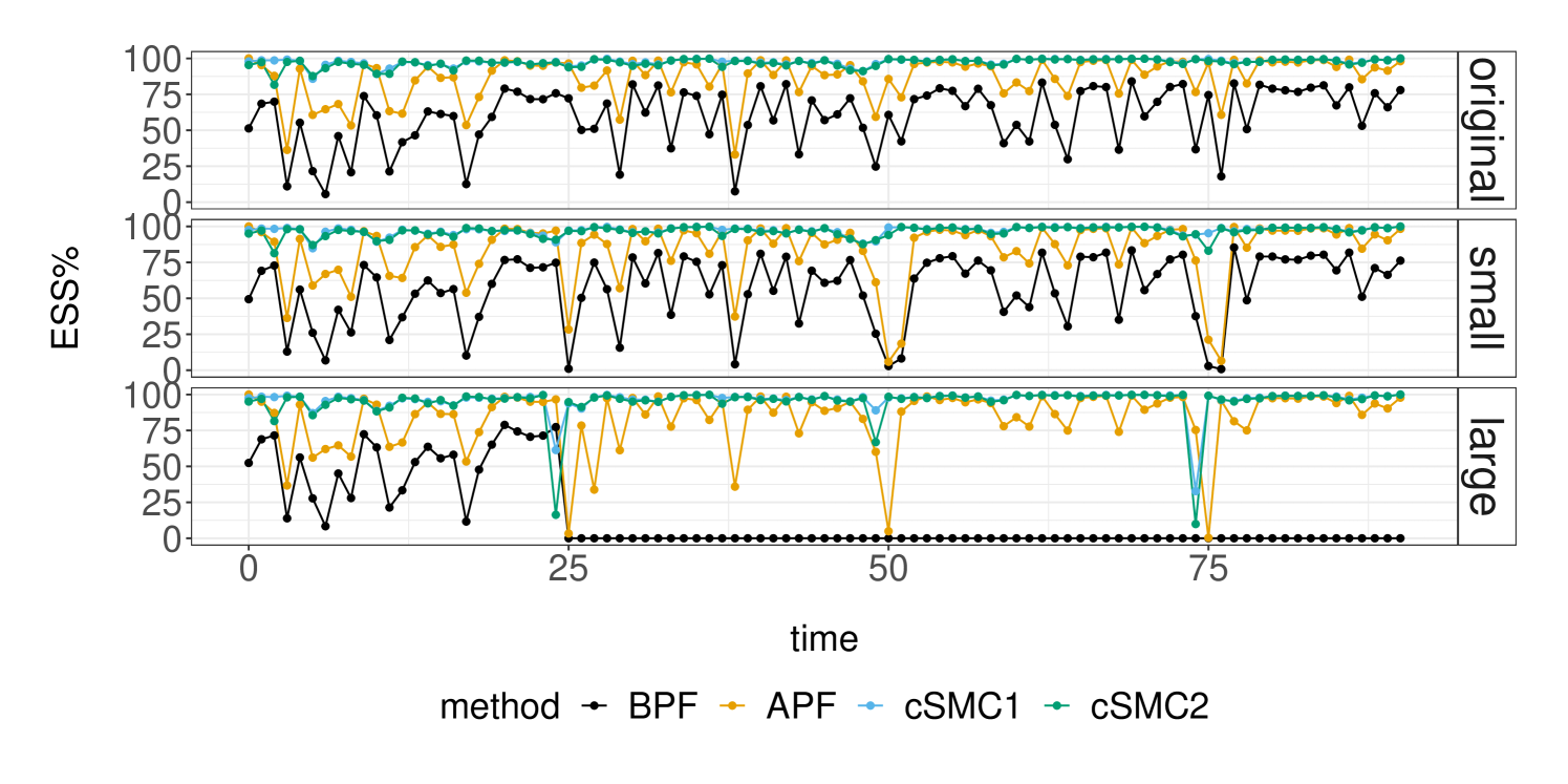
The top panel of Figure 2 illustrates the performance of these SMC methods at the data-generating parameter (DGP), measured in terms of the effective sample size (ESS) criterion (Kong et al., 1994). The ESS at time t[0:T]t\in[0:T], defined in terms of the normalized weights (Wt(p))p[1:P](W_{t}^{(p)})_{p\in[1:P]} as 1/p=1P(Wt(p))21/\sum_{p=1}^{P}(W_{t}^{(p)})^{2}, measures the adequacy of the importance sampling approximation at each step. We consider two implementations of the controlled SMC in Algorithm 3: cSMC1 employs proposal distributions that are defined by the BIF approximation in Algorithm 2, while cSMC2 relies on translated Poisson approximations of the SumBin distributions in Algorithm 2 to lower the computational cost. This lowers the run-time of the BIF approximation from 0.350.35 to 0.120.12 second, which are insignificant relative to the cost of cSMC for a population size of N=100N=100. As expected, the APF performs better than the BPF by taking the next observation into account, and cSMC does better than APF by incorporating information from the entire observation sequence. Furthermore, the faster BIF approximation does not result in a noticeable loss of cSMC performance due to the accuracy of the translated Poisson approximations with N=100N=100 agents. Although the performance of BPF seems adequate in this simulated data setting, the middle and bottom panels of Figure 2 reveal that its particle approximation can collapse whenever there are smaller or larger observation counts. In contrast, the performance of APF and cSMC appear to be more robust to such informative observations.

Refer to caption
Figure 2: Effective sample size of various SMC methods with P=512P=512 particles when considering simulated observations (top), when observations at t{25,50,75}t\in\{25,50,75\} are replaced by yt/2\lfloor y_{t}/2\rfloor (middle), or min(2yt,N)\min(2y_{t},N) (bottom).

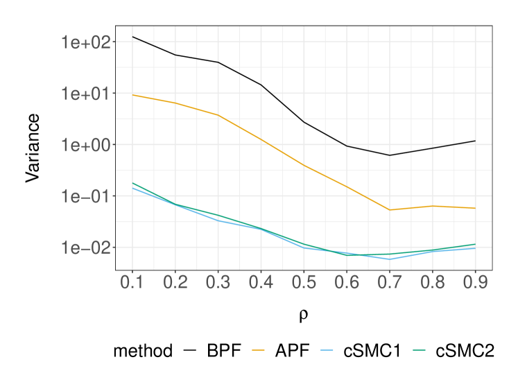
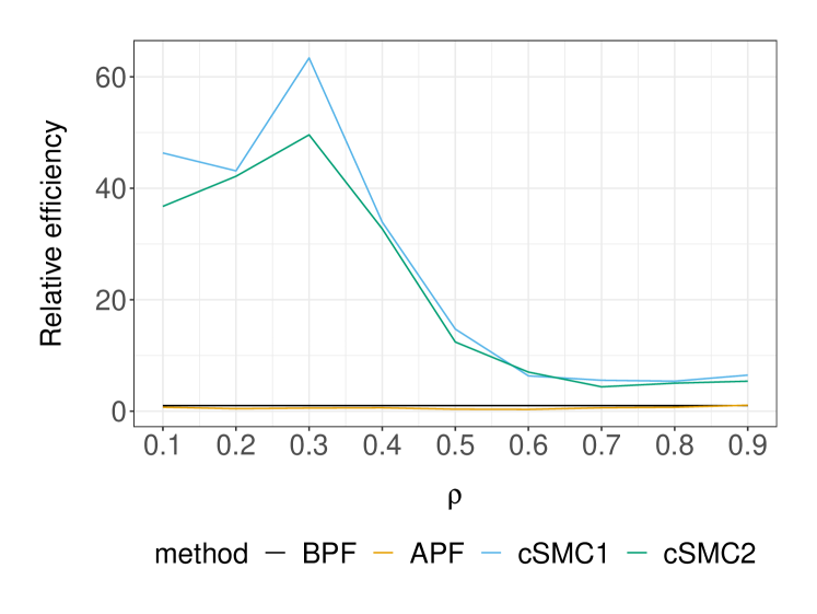
Next we examine the performance of these SMC methods in terms of marginal likelihood estimation. Table 2 displays the variance of the log-marginal likelihood estimator at two parameter sets, and its average cost measured as run-time that were estimated using 100100 independent repetitions of each method. At the DGP, it is apparent that the cSMC estimators achieve the asymptotic regime of PP\rightarrow\infty earlier than BPF and APF, which seem to require at least P=512P=512 particles. Based on the largest value of PP that we considered, the asymptotic variance of APF, cSMC1 and cSMC2 was found to be 2929, 155155 and 115115 times smaller relative to BPF, respectively. As the cost of APF and cSMC was approximately 1919 times more expensive than BPF in our implementation, we see that APF, cSMC1 and cSMC2 are respectively 1.51.5, 88 and 66 times more efficient than BPF at the DGP. We can expect these efficiency gains to be more significant as we move away from the DGP. To illustrate this, we consider another parameter set which has βλ=(3,0)\beta_{\lambda}=(-3,0) and keeps all other parameters at the DGP. Although this is a less likely set of parameters as the log-marginal likelihood is approximately 232232 lower than the DGP, adequate marginal likelihood estimation is crucial when employing SMC methods within particle MCMC algorithms for parameter inference. In this case, we found that the BPF marginal likelihood estimates could collapse to zero for the values of PP that are considered in Table 2. In contrast, APF and cSMC would not suffer from this issue by construction. By increasing the number of BPF particles to P=262,144P=262,144 and comparing its performance to APF, cSMC1 and cSMC2 with P=2048P=2048 particles, we find that BPF is respectively 99, 7676 and 4242 times less efficient at this parameter set. Lastly, Figure 3 illustrates the comparison of SMC methods as the parameter ρ\rho varies and all other parameters fixed at the DGP.

BPF APF cSMC1 cSMC2
PP DGP Cost DGP Non-DGP Cost DGP Non-DGP DGP Non-DGP Cost
Var (sec) Var Var (sec) Var Var Var Var (sec)
64 4.32 0.09 0.281 71.88 1.49 0.0696 13.52 0.0779 18.44 1.46
128 2.39 0.17 0.154 39.52 2.95 0.0285 8.62 0.0382 8.48 2.88
256 1.67 0.33 0.110 26.86 5.85 0.0164 4.11 0.0190 6.88 5.72
512 0.88 0.63 0.056 18.98 11.72 0.0087 3.57 0.0105 5.03 11.41
1024 0.55 1.25 0.026 13.38 23.46 0.0049 2.05 0.0046 3.41 22.83
2048 0.31 2.49 0.011 9.93 47.48 0.0020 1.15 0.0027 2.07 45.97
Table 2: Variance of log-marginal likelihood estimator and its average cost (in seconds) using different number of particles PP and various SMC methods. The parameter sets considered are the data generating parameters (DGP) and a modification of the DGP with βλ=(3,0)\beta_{\lambda}=(-3,0) (labelled as non-DGP). The cost of cSMC1 and cSMC2 are comparable and the run-times to compute the BIF approximations (0.35 and 0.12 second for cSMC1 and cSMC2) are not reported in this table.
Refer to caption
Refer to caption
Figure 3: Variance of log-marginal likelihood estimator (left) and relative efficiency (right) of various SMC methods compared to the BPF with P=512P=512 particles, as ρ\rho varies and the other parameters fixed at the DGP.

3.4 Parameter and state inference

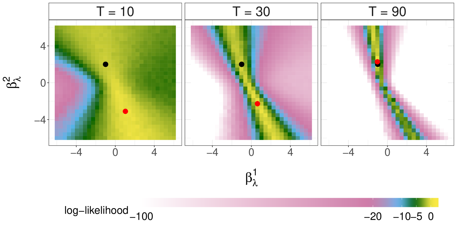
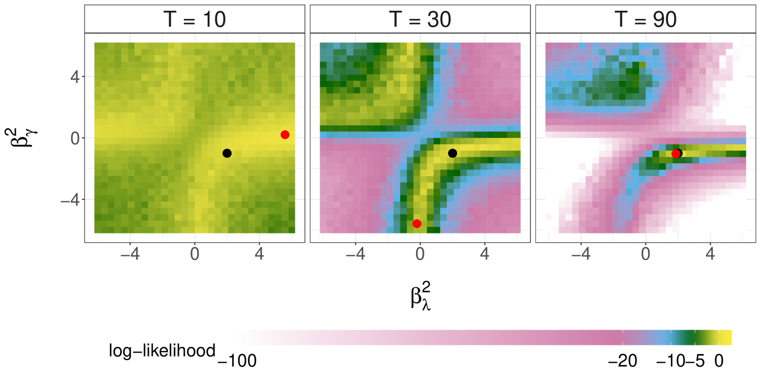
We first concern ourselves with the behaviour of the marginal likelihood and the maximum likelihood estimator (MLE) argmaxθΘpθ(y0:T)\arg\max_{\theta\in\Theta}p_{\theta}(y_{0:T}) as the number of observations TT\rightarrow\infty. This is illustrated with our running simulated dataset from Section 3.3. Figure 4 plots the log-likelihood as a function of βλ=(βλ1,βλ2)\beta_{\lambda}=(\beta_{\lambda}^{1},\beta_{\lambda}^{2}) or (βλ2,βγ2)(\beta_{\lambda}^{2},\beta_{\gamma}^{2}) with the other parameters fixed at their data generating values, estimated using cSMC with P=64P=64 particles. These plots reveal the complex behavior of the likelihood functions induced by agent-based SIS models. Furthermore, we see that the likelihood concentrates more around the DGP as TT increases, and that the MLE can recover the DGP when TT is sufficiently large.

Refer to caption
Refer to caption
Figure 4: Estimated log-likelihood as a function of βλ=(βλ1,βλ2)\beta_{\lambda}=(\beta_{\lambda}^{1},\beta_{\lambda}^{2}) (first row) or (βλ2,βγ2)(\beta_{\lambda}^{2},\beta_{\gamma}^{2}) (second row) with the other parameters fixed at the DGP given t{10,30,90}t\in\{10,30,90\} observations. For ease of plotting, the log-likelihood values were translated so that the MLE (red dot) attains a maximum of zero. The data generating parameters of βλ=(1,2)\beta_{\lambda}=(-1,2) or (βλ2,βγ2)=(2,1)(\beta_{\lambda}^{2},\beta_{\gamma}^{2})=(2,-1) are shown as a black dot.

By building on the SMC methods in Sections 3.1 and 3.2, one can construct a stochastic gradient ascent scheme or an expectation-maximization algorithm to approximate the MLE. We refer readers to Kantas et al. (2015) for a comprehensive review of such approaches. In the Bayesian framework, our interest is on the posterior distribution

p(θ,x0:T|y0:T)=p(θ|y0:T)pθ(x0:T|y0:T)p(θ)pθ(x0:T,y0:T),\displaystyle p(\theta,x_{0:T}|y_{0:T})=p(\theta|y_{0:T})p_{\theta}(x_{0:T}|y_{0:T})\propto p(\theta)p_{\theta}(x_{0:T},y_{0:T}), (44)

where p(dθ)=p(θ)dθp(d\theta)=p(\theta)d\theta is a given prior distribution on the parameter space Θ\Theta. We employ particle marginal Metropolis–Hastings (PMMH) to sample from the posterior distribution. Following the discussion in Section 3.3, we will choose cSMC to construct a more efficient PMMH chain.

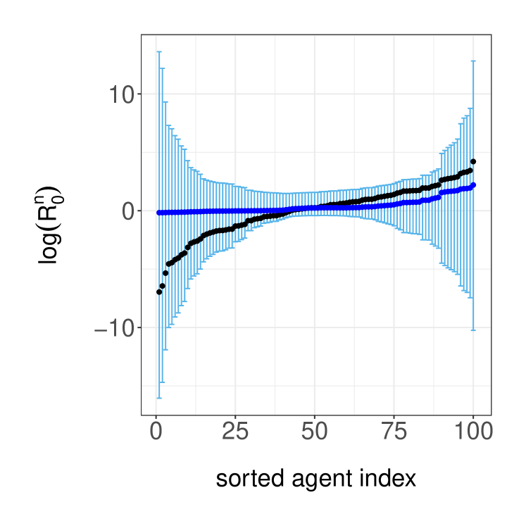
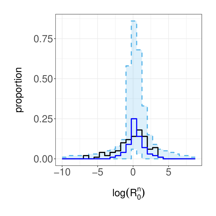
We now illustrate our inference method on the simulated data setup of Section 3.3. We adopt a prior distribution that assumes the parameters are independent with β0,βλ,βγ𝒩(0,9)\beta_{0},\beta_{\lambda},\beta_{\gamma}\sim\mathcal{N}(0,9) and ρUniform(0,1)\rho\sim\text{Uniform}(0,1). All MH parameter updates employ a Normal random walk proposal transition on the (β0,βλ,βγ,log(ρ/(1ρ)))(\beta_{0},\beta_{\lambda},\beta_{\gamma},\log(\rho/(1-\rho)))-space, with a standard deviation of 0.20.2 to achieve suitable acceptance probabilities. We use P=128P=128 particles in the cSMC algorithm within PMMH and we run the PMMH algorithm for 100,000100,000 iterations after a burn in of 50005000 iterations. Using these posterior samples, we infer the ratios R0n=λn/γnR_{0}^{n}=\lambda^{n}/\gamma^{n}, which can be understood as the reproductive number of agent n[1:N]n\in[1:N]. In the left panel of Figure 5, we display the estimated posterior medians and 95%95\% credible sets, as well as the data generating values. Although the posterior median estimates are similar across agents, there is large posterior uncertainty for agents with small or large data generated ratios. To visualize how (R0n)n[1:N](R_{0}^{n})_{n\in[1:N]} is distributed in the population, we estimate histograms that take parameter uncertainty into account, illustrate the results in the right panel of Figure 5. The posterior median estimates yields a histogram that is more concentrated than its data generating counterpart.

Refer to caption
Refer to caption
Figure 5: Posterior estimates of the reproductive number R0n=λn/γnR_{0}^{n}=\lambda^{n}/\gamma^{n} of each agent n[1:N]n\in[1:N] (left) and its distribution in the population (right). Posterior medians are shown in blue and the 95%95\% posterior credible sets in light blue. Data generating values are illustrated in black.

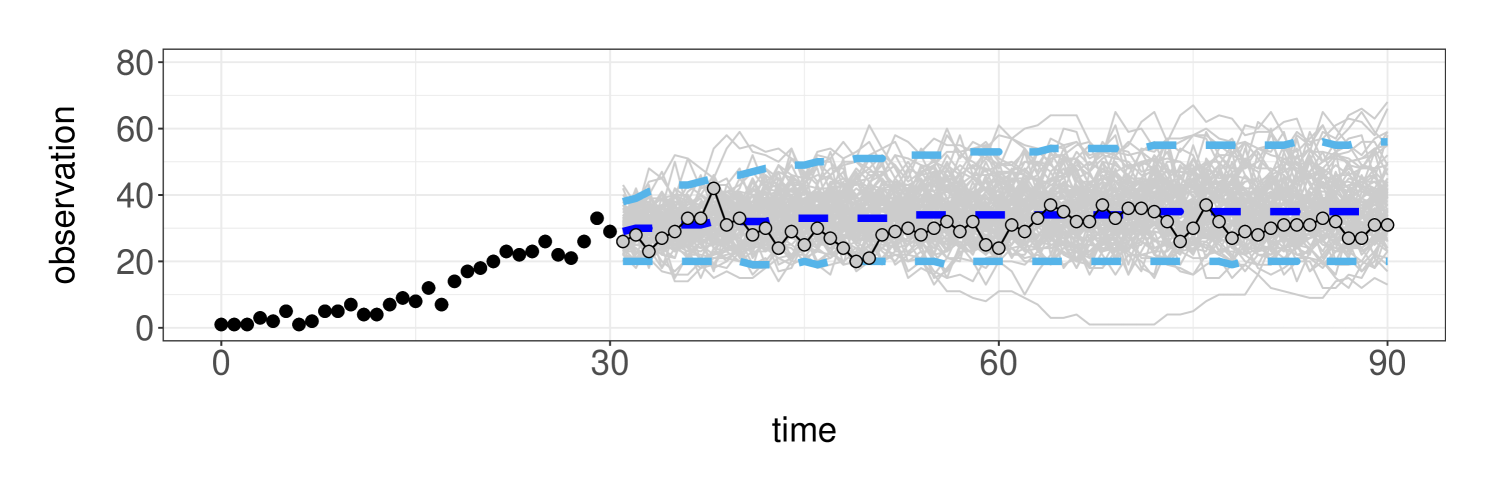
Lastly, we examine the predictive performance of the model when relatively few observations are available. As illustrated in Figure 6, we assume access to the first t=30t=30 observations (black dots) and predict the rest of the time series up to time T=90T=90 (grey dots) using the posterior predictive distribution p(yt+1:T|y0:t)=Θxt{0,1}Npθ(yt+1:T|xt)p(θ,xt|y0:t)p(y_{t+1:T}|y_{0:t})=\int_{\Theta}\sum_{x_{t}\in\{0,1\}^{N}}p_{\theta}(y_{t+1:T}|x_{t})p(\theta,x_{t}|y_{0:t}). By simulating trajectories from the posterior predictive (grey lines), we obtain the model predictions and uncertainty estimates in Figure 6.

Refer to caption
Figure 6: Observation sequence plotted as dots that are coloured initially in black followed by grey from time t=30t=30 to T=90T=90. Some sampled trajectories from the posterior predictive distribution p(yt+1:T|y0:t)p(y_{t+1:T}|y_{0:t}) are depicted as grey lines. The blue dashed line shows the medians over time; the lower and upper light blue dashed lines correspond to the 2.5%2.5\% and 97.5%97.5\% quantiles respectively.

4 Susceptible-Infected-Recovered model

We consider a susceptible-infected-recovered (SIR) model, where agents become immune to a pathogen after they recover from an infection. The “recovered” status of an agent shall be encoded by a state of 22. Given a population configuration x=(xn)n[1:N]{0,1,2}Nx=(x^{n})_{n\in[1:N]}\in\{0,1,2\}^{N}, we will write Sn(x)=𝟙(xn=0)S^{n}(x)=\mathbbm{1}(x^{n}=0), In(x)=𝟙(xn=1)I^{n}(x)=\mathbbm{1}(x^{n}=1), Rn(x)=𝟙(xn=2)R^{n}(x)=\mathbbm{1}(x^{n}=2) to indicate the status of agent n[1:N]n\in[1:N], and S(x)=n=1NSn(x)S(x)=\sum_{n=1}^{N}S^{n}(x), I(x)=n=1NIn(x)I(x)=\sum_{n=1}^{N}I^{n}(x), R(x)=n=1NRn(x)R(x)=\sum_{n=1}^{N}R^{n}(x) to count the number of agents in each state. Under the assumption of a closed population, we have S(x)+I(x)+R(x)=NS(x)+I(x)+R(x)=N.

The time evolution of the population (Xt)t[0:T](X_{t})_{t\in[0:T]} is now modelled by a Markov chain on {0,1,2}N\{0,1,2\}^{N}, i.e. the specification in (18) with

μθ(x0)=n=1NCat(x0n;[0:2],α0n),fθ(xt|xt1)=n=1NCat(xtn;[0:2],αn(xt1)),t[1:T].\displaystyle\mu_{\theta}(x_{0})=\prod_{n=1}^{N}\text{Cat}(x_{0}^{n};[0:2],\alpha_{0}^{n}),\quad f_{\theta}(x_{t}|x_{t-1})=\prod_{n=1}^{N}\text{Cat}(x_{t}^{n};[0:2],\alpha^{n}(x_{t-1})),\quad t\in[1:T]. (45)

The above probabilities are given by α0n=(α0,Sn,α0,In,α0,Rn)=(1α0,In,α0,In,0)\alpha_{0}^{n}=(\alpha_{0,S}^{n},\alpha_{0,I}^{n},\alpha_{0,R}^{n})=(1-\alpha_{0,I}^{n},\alpha_{0,I}^{n},0) and αn(xt1)=(αSn(xt1),αIn(xt1),αRn(xt1))\alpha^{n}(x_{t-1})=(\alpha_{S}^{n}(x_{t-1}),\alpha_{I}^{n}(x_{t-1}),\alpha_{R}^{n}(x_{t-1})) where

αSn(xt1)=Sn(xt1)(1λn𝒟(n)1m𝒩(n)Im(xt1)),\displaystyle\alpha_{S}^{n}(x_{t-1})=S^{n}(x_{t-1})\left(1-\lambda^{n}\mathcal{D}(n)^{-1}\sum_{m\in\mathcal{N}(n)}I^{m}(x_{t-1})\right),
αIn(xt1)=Sn(xt1)λn𝒟(n)1m𝒩(n)Im(xt1)+In(xt1)(1γn),\displaystyle\alpha_{I}^{n}(x_{t-1})=S^{n}(x_{t-1})\lambda^{n}\mathcal{D}(n)^{-1}\sum_{m\in\mathcal{N}(n)}I^{m}(x_{t-1})+I^{n}(x_{t-1})(1-\gamma^{n}), (46)
αRn(xt1)=In(xt1)γn+Rn(xt1),\displaystyle\alpha_{R}^{n}(x_{t-1})=I^{n}(x_{t-1})\gamma^{n}+R^{n}(x_{t-1}),

which satisfies αSn(xt1)+αIn(xt1)+αRn(xt1)=1\alpha_{S}^{n}(x_{t-1})+\alpha_{I}^{n}(x_{t-1})+\alpha_{R}^{n}(x_{t-1})=1. Note that αRn(xt1)=1\alpha_{R}^{n}(x_{t-1})=1 if Rn(xt1)=1R^{n}(x_{t-1})=1, which reflects the above-mentioned immunity. Just like the SIS model, the agents’ initial infection probabilities, infection and recovery rates (α0,In,λn,γn)n[1:N](\alpha_{0,I}^{n},\lambda^{n},\gamma^{n})_{n\in[1:N]} are specified with (17), and the observation model for the number of infections reported over time (Yt)t[0:T](Y_{t})_{t\in[0:T]} is (3).

We consider again SMC approximations of the marginal likelihood and smoothing distribution of the resulting hidden Markov model on {0,1,2}N\{0,1,2\}^{N}. The BPF can be readily implemented in 𝒪(NTP)\mathcal{O}(NTP) cost, but suffers from the difficulties discussed in Section 3.1. To obtain better performance, we discuss how to implement the fully adapted APF in Section 4.1 and adapt our cSMC construction in Section 4.2. Alternative MCMC approaches such as those detailed in Appendix C could also be considered.

4.1 Auxiliary particle filter

We recall that implementing the fully adapted APF requires one to sample from proposals q0(x0|θ)=pθ(x0|y0),qt(xt|xt1,θ)=pθ(xt|xt1,yt)q_{0}(x_{0}|\theta)=p_{\theta}(x_{0}|y_{0}),q_{t}(x_{t}|x_{t-1},\theta)=p_{\theta}(x_{t}|x_{t-1},y_{t}) for t[1:T]t\in[1:T], and evaluate the weight functions w0(x0)=pθ(y0)w_{0}(x_{0})=p_{\theta}(y_{0}) and wt(xt1)=pθ(yt|xt1)w_{t}(x_{t-1})=p_{\theta}(y_{t}|x_{t-1}) for t[1:T]t\in[1:T]. At the initial time, we compute the marginal likelihood pθ(y0)p_{\theta}(y_{0}) as

pθ(y0)=i0=0NPoiBin(i0;α0,I)Bin(y0;i0,ρ)𝟙(i0y0)\displaystyle p_{\theta}(y_{0})=\sum_{i_{0}=0}^{N}\text{PoiBin}(i_{0};\alpha_{0,I})\text{Bin}(y_{0};i_{0},\rho)\mathbbm{1}(i_{0}\geq y_{0}) (47)

where α0,I=(α0,In)n[1:N]\alpha_{0,I}=(\alpha_{0,I}^{n})_{n\in[1:N]}, and sample from

pθ(x0,i0,i01:N|y0)=pθ(i0|y0)pθ(i01:N|i0)pθ(x0|i01:N)\displaystyle p_{\theta}(x_{0},i_{0},i_{0}^{1:N}|y_{0})=p_{\theta}(i_{0}|y_{0})p_{\theta}(i_{0}^{1:N}|i_{0})p_{\theta}(x_{0}|i_{0}^{1:N}) (48)
=PoiBin(i0;α0,I)Bin(y0;i0,ρ)𝟙(i0y0)pθ(y0)CondBer(i01:N;α0,I,i0)n=1NCat(x0n;[0:2],ν0(i0n))\displaystyle=\frac{\text{PoiBin}(i_{0};\alpha_{0,I})\text{Bin}(y_{0};i_{0},\rho)\mathbbm{1}(i_{0}\geq y_{0})}{p_{\theta}(y_{0})}\text{CondBer}(i_{0}^{1:N};\alpha_{0,I},i_{0})\prod_{n=1}^{N}\text{Cat}(x_{0}^{n};[0:2],\nu_{0}(i_{0}^{n}))

with ν0(i0n)=(1i0n,i0n,0)\nu_{0}(i_{0}^{n})=(1-i_{0}^{n},i_{0}^{n},0), which admits the posterior of agent states pθ(x0|y0)p_{\theta}(x_{0}|y_{0}) as its marginal distribution. Similarly, for time step t[1:T]t\in[1:T], we compute the predictive likelihood pθ(yt|xt1)p_{\theta}(y_{t}|x_{t-1}) as

pθ(yt|xt1)=it=0NPoiBin(it;αI(xt1))Bin(yt;it,ρ)𝟙(ityt)\displaystyle p_{\theta}(y_{t}|x_{t-1})=\sum_{i_{t}=0}^{N}\text{PoiBin}(i_{t};\alpha_{I}(x_{t-1}))\text{Bin}(y_{t};i_{t},\rho)\mathbbm{1}(i_{t}\geq y_{t}) (49)

where αI(xt1)=(αIn(xt1))n[1:N]\alpha_{I}(x_{t-1})=(\alpha_{I}^{n}(x_{t-1}))_{n\in[1:N]}, and sample from

pθ(xt,it,it1:N|xt1,yt)=pθ(it|xt1,yt)pθ(it1:N|xt1,it)pθ(xt|xt1,it1:N)\displaystyle p_{\theta}(x_{t},i_{t},i_{t}^{1:N}|x_{t-1},y_{t})=p_{\theta}(i_{t}|x_{t-1},y_{t})p_{\theta}(i_{t}^{1:N}|x_{t-1},i_{t})p_{\theta}(x_{t}|x_{t-1},i_{t}^{1:N}) (50)
=PoiBin(it;αI(xt1))Bin(yt;it,ρ)𝟙(ityt)pθ(yt|xt1)CondBer(it1:N;αI(xt1),it)n=1NCat(xtn;[0:2],ν(xt1,itn))\displaystyle=\frac{\text{PoiBin}(i_{t};\alpha_{I}(x_{t-1}))\text{Bin}(y_{t};i_{t},\rho)\mathbbm{1}(i_{t}\geq y_{t})}{p_{\theta}(y_{t}|x_{t-1})}\text{CondBer}(i_{t}^{1:N};\alpha_{I}(x_{t-1}),i_{t})\prod_{n=1}^{N}\text{Cat}(x_{t}^{n};[0:2],\nu(x_{t-1},i_{t}^{n}))

with ν(xt1,itn)=((1itn)Sn(xt1),itn,(1itn){In(xt1)+Rn(xt1)})\nu(x_{t-1},i_{t}^{n})=((1-i_{t}^{n})S^{n}(x_{t-1}),i_{t}^{n},(1-i_{t}^{n})\{I^{n}(x_{t-1})+R^{n}(x_{t-1})\}), which admits pθ(xt|xt1,yt)p_{\theta}(x_{t}|x_{t-1},y_{t}) as its marginal transition.

By augmenting the infection status of the agents I1:N(xt)=(In(xt))n[1:N]I^{1:N}(x_{t})=(I^{n}(x_{t}))_{n\in[1:N]}, the first two steps in (48) and (50) are analogous to (25) and (27) for the SIS model, and the last step is to identify an agent’s state given her augmented current infection status and previous state. We point out that ν0(i0n),ν(xt1,itn){(1,0,0),(0,1,0),(0,0,1)}.\nu_{0}(i_{0}^{n}),\nu(x_{t-1},i_{t}^{n})\in\{(1,0,0),(0,1,0),(0,0,1)\}. These expressions for ν0(i0n)\nu_{0}(i_{0}^{n}) and ν(xt1,itn)\nu(x_{t-1},i_{t}^{n}) exploit the following facts: (ii) susceptible agents either remain susceptible or become infected; (iiii) infected agents either remain infected or recover; (iiiiii) agents who have recovered enjoy immunity. Algorithm 4 provides an algorithmic description of the resulting APF, which has the same cost as APF for the SIS model.

Input: Parameters θΘ\theta\in\Theta and number of particles PP\in\mathbb{N}
compute v0(i)=PoiBin(i;α0,I)Bin(y0;i,ρ)𝟙(iy0)v_{0}^{(i)}=\text{PoiBin}(i;\alpha_{0,I})\text{Bin}(y_{0};i,\rho)\mathbbm{1}(i\geq y_{0}) for i[0:N]i\in[0:N]
set w0=i=0Nv0(i)w_{0}=\sum_{i=0}^{N}v_{0}^{(i)}
normalize V0(i)=v0(i)/w0V_{0}^{(i)}=v_{0}^{(i)}/w_{0} for i[0:N]i\in[0:N]
sample I0(p)Cat([0:N],V0(0:N))I_{0}^{(p)}\sim\text{Cat}([0:N],V_{0}^{(0:N)}), I01:N,(p)|I0(p)CondBer(α0,I,I0(p))I_{0}^{1:N,(p)}|I_{0}^{(p)}\sim\text{CondBer}(\alpha_{0,I},I_{0}^{(p)}) for p[1:P]p\in[1:P]
sample X0n,(p)|I0n,(p)Cat([0:2],ν0(I0n,(p)))X_{0}^{n,(p)}|I_{0}^{n,(p)}\sim\text{Cat}([0:2],\nu_{0}(I_{0}^{n,(p)})) for p[1:P]p\in[1:P] and n[1:N]n\in[1:N]
for t=1,,Tt=1,\cdots,T and p=1,,Pp=1,\cdots,P do
   compute vt(i,p)=PoiBin(i;αI(Xt1(p)))Bin(yt;i,ρ)𝟙(iyt)v_{t}^{(i,p)}=\text{PoiBin}(i;\alpha_{I}(X_{t-1}^{(p)}))\text{Bin}(y_{t};i,\rho)\mathbbm{1}(i\geq y_{t}) for i[0:N]i\in[0:N]
   set wt(p)=i=0Nvt(i,p)w_{t}^{(p)}=\sum_{i=0}^{N}v_{t}^{(i,p)}
   normalize Vt(i,p)=vt(i,p)/wt(p)V_{t}^{(i,p)}=v_{t}^{(i,p)}/w_{t}^{(p)} for i[0:N]i\in[0:N]
   normalize Wt(p)=wt(p)/k=1Pwt(k)W_{t}^{(p)}=w_{t}^{(p)}/\sum_{k=1}^{P}w_{t}^{(k)}
   sample At1(p)r(|Wt(1:P))A_{t-1}^{(p)}\sim r(\cdot|W_{t}^{(1:P)})
   sample It(p)Cat([0:N],Vt(0:N,At1(p)))I_{t}^{(p)}\sim\text{Cat}([0:N],V_{t}^{(0:N,A_{t-1}^{(p)})}) and It1:N,(p)|It(p)CondBer(αI(Xt1(At1(p))),It(p))I_{t}^{1:N,(p)}|I_{t}^{(p)}\sim\text{CondBer}(\alpha_{I}(X_{t-1}^{(A_{t-1}^{(p)})}),I_{t}^{(p)})
   sample Xtn,(p)Xt1(At1(p)),Itn,(p)Cat([0:2],ν(Xt1(At1(p)),Itn,(p)))X_{t}^{n,(p)}\mid X_{t-1}^{(A_{t-1}^{(p)})},I_{t}^{n,(p)}\sim\text{Cat}([0:2],\nu(X_{t-1}^{(A_{t-1}^{(p)})},I_{t}^{n,(p)})) for n[1:N]n\in[1:N]
end for
Output: Marginal likelihood estimator p^θ(y0:T)=w0t=1TP1p=1Pwt(p)\hat{p}_{\theta}(y_{0:T})=w_{0}\prod_{t=1}^{T}P^{-1}\sum_{p=1}^{P}w_{t}^{(p)}, states (Xt(p))(t,p)[0:T]×[1:P](X_{t}^{(p)})_{(t,p)\in[0:T]\times[1:P]} and ancestors (At(p))(t,p)[0:T1]×[1:P](A_{t}^{(p)})_{(t,p)\in[0:T-1]\times[1:P]}
Algorithm 4 Auxiliary particle filter for SIR model

4.2 Controlled sequential Monte Carlo

We now consider approximation of the BIF (30) to construct a proposal distribution approximating (29). At the terminal time TT, it suffices to compute ψT(iT)=Bin(yT;iT,ρ)𝟙(iTyT)\psi_{T}(i_{T})=\text{Bin}(y_{T};i_{T},\rho)\mathbbm{1}(i_{T}\geq y_{T}) for all iT[0:N]i_{T}\in[0:N] to represent the function ψT(xT)\psi_{T}^{\star}(x_{T}). As before, the next iterate ψT1(xT1)\psi_{T-1}^{\star}(x_{T-1}) requires an approximation of the conditional expectation fθ(ψT|xT1)=iT=0NPoiBin(iT;αI(xT1))ψT(iT)f_{\theta}(\psi_{T}|x_{T-1})=\sum_{i_{T}=0}^{N}\text{PoiBin}(i_{T};\alpha_{I}(x_{T-1}))\psi_{T}(i_{T}). Following the arguments in (31), we approximate α(xT1)\alpha(x_{T-1}) by

α¯n(xT1)=(α¯Sn(xT1),α¯In(xT1),α¯Rn(xT1)),\displaystyle\bar{\alpha}^{n}(x_{T-1})=(\bar{\alpha}_{S}^{n}(x_{T-1}),\bar{\alpha}_{I}^{n}(x_{T-1}),\bar{\alpha}_{R}^{n}(x_{T-1})),

defined as

α¯Sn(xT1)=Sn(xT1)(1λ¯N1I(xT1)),\displaystyle\bar{\alpha}_{S}^{n}(x_{T-1})=S^{n}(x_{T-1})\left(1-\bar{\lambda}N^{-1}I(x_{T-1})\right),
α¯In(xT1)=Sn(xT1)λ¯N1I(xT1)+In(xT1)(1γ¯),\displaystyle\bar{\alpha}_{I}^{n}(x_{T-1})=S^{n}(x_{T-1})\bar{\lambda}N^{-1}I(x_{T-1})+I^{n}(x_{T-1})(1-\bar{\gamma}), (51)
α¯Rn(xT1)=In(xT1)γ¯+Rn(xT1),\displaystyle\bar{\alpha}_{R}^{n}(x_{T-1})=I^{n}(x_{T-1})\bar{\gamma}+R^{n}(x_{T-1}),

which satisfies α¯Sn(xT1)+α¯In(xT1)+α¯Rn(xT1)=1\bar{\alpha}_{S}^{n}(x_{T-1})+\bar{\alpha}_{I}^{n}(x_{T-1})+\bar{\alpha}_{R}^{n}(x_{T-1})=1. Writing the corresponding Markov transition as f¯θ(xT|xT1)=n=1NCat(xTn;[0:2],α¯n(xT1))\bar{f}_{\theta}(x_{T}|x_{T-1})=\prod_{n=1}^{N}\text{Cat}(x_{T}^{n};[0:2],\bar{\alpha}^{n}(x_{T-1})), we approximate the conditional expectation fθ(ψT|xT1)f_{\theta}(\psi_{T}|x_{T-1}) by

f¯θ(ψT|S(xT1),I(xT1))=iT=0NSumBin(iT;S(xT1),λ¯N1I(xT1),I(xT1),1γ¯)ψT(iT).\displaystyle\bar{f}_{\theta}(\psi_{T}|S(x_{T-1}),I(x_{T-1}))=\sum_{i_{T}=0}^{N}\text{SumBin}(i_{T};S(x_{T-1}),\bar{\lambda}N^{-1}I(x_{T-1}),I(x_{T-1}),1-\bar{\gamma})\psi_{T}(i_{T}). (52)

Although (52) is analogous to (32) for the SIS model, the number of susceptible agents S(xT1)S(x_{T-1}) cannot be determined by just knowing the number of infections I(xT1)I(x_{T-1}) in the SIR model. Therefore it is necessary to account for both S(xT1)S(x_{T-1}) and I(xT1)I(x_{T-1}) in our approximation, i.e. we compute

ψT1(sT1,iT1)=Bin(yT1;iT1,ρ)𝟙(iT1yT1)f¯θ(ψT|sT1,iT1)\displaystyle\psi_{T-1}(s_{T-1},i_{T-1})=\text{Bin}(y_{T-1};i_{T-1},\rho)\mathbbm{1}(i_{T-1}\geq y_{T-1})\bar{f}_{\theta}(\psi_{T}|s_{T-1},i_{T-1}) (53)

for all (sT1,iT1)[0:N]×[0:(NsT1)](s_{T-1},i_{T-1})\in[0:N]\times[0:(N-s_{T-1})]. Since the number of agents in the population is fixed, it is also possible to work with the variables I(xT1)I(x_{T-1}) and R(xT1)R(x_{T-1}) instead. Subsequently for t[0:T2]t\in[0:T-2], we approximate (30) by

ψt(st,it)=Bin(yt;it,ρ)𝟙(ityt)f¯θ(ψt+1|st,it),(st,it)[0:N]×[0:(Nst)],\displaystyle\psi_{t}(s_{t},i_{t})=\text{Bin}(y_{t};i_{t},\rho)\mathbbm{1}(i_{t}\geq y_{t})\bar{f}_{\theta}(\psi_{t+1}|s_{t},i_{t}),\quad(s_{t},i_{t})\in[0:N]\times[0:(N-s_{t})], (54)

where f¯θ(ψt+1|st,it)=st+1=0Nit+1=0Nst+1f¯θ(st+1,it+1|st,it)ψt+1(st+1,it+1)\bar{f}_{\theta}(\psi_{t+1}|s_{t},i_{t})=\sum_{s_{t+1}=0}^{N}\sum_{i_{t+1}=0}^{N-s_{t+1}}\bar{f}_{\theta}(s_{t+1},i_{t+1}|s_{t},i_{t})\psi_{t+1}(s_{t+1},i_{t+1}),

f¯θ(st+1,it+1|st,it)=Bin(st+1;st,1λ¯N1it)Bin(itit+1+stst+1;it,γ¯),\displaystyle\bar{f}_{\theta}(s_{t+1},i_{t+1}|s_{t},i_{t})=\text{Bin}(s_{t+1};s_{t},1-\bar{\lambda}N^{-1}i_{t})\text{Bin}(i_{t}-i_{t+1}+s_{t}-s_{t+1};i_{t},\bar{\gamma}), (55)

for (st+1,it+1)[0:st]×[(stst+1):(it+stst+1)](s_{t+1},i_{t+1})\in[0:s_{t}]\times[(s_{t}-s_{t+1}):(i_{t}+s_{t}-s_{t+1})], and zero otherwise. The above expression follows from the SIR model structure under homogeneous probabilities (4.2). Algorithm 5 summarizes our approximation of the BIF (ψt)t[0:T](\psi_{t})_{t\in[0:T]}, which costs 𝒪(N4T)\mathcal{O}(N^{4}T) to compute and 𝒪(N2T)\mathcal{O}(N^{2}T) in storage.

Input: Parameters θΘ\theta\in\Theta
compute ψT(iT)=Bin(yT;iT,ρ)𝟙(iTyT)\psi_{T}(i_{T})=\text{Bin}(y_{T};i_{T},\rho)\mathbbm{1}(i_{T}\geq y_{T}) for iT[0:N]i_{T}\in[0:N]
for t=T1,,0t=T-1,\cdots,0, st=0,,Ns_{t}=0,\ldots,N and it=0,,Nsti_{t}=0,\cdots,N-s_{t} do
 if t=T1t=T-1 then
      compute f¯θ(ψt+1|st,it)=it+1=0NSumBin(it+1;st,λ¯N1it,it,1γ¯)ψt+1(it+1)\bar{f}_{\theta}(\psi_{t+1}|s_{t},i_{t})=\sum_{i_{t+1}=0}^{N}\text{SumBin}(i_{t+1};s_{t},\bar{\lambda}N^{-1}i_{t},i_{t},1-\bar{\gamma})\psi_{t+1}(i_{t+1})
    
 else
      compute f¯θ(ψt+1|st,it)=st+1=0Nit+1=0Nst+1f¯θ(st+1,it+1|it,st)ψt+1(st+1,it+1)\bar{f}_{\theta}(\psi_{t+1}|s_{t},i_{t})=\sum_{s_{t+1}=0}^{N}\sum_{i_{t+1}=0}^{N-s_{t+1}}\bar{f}_{\theta}(s_{t+1},i_{t+1}|i_{t},s_{t})\psi_{t+1}(s_{t+1},i_{t+1})
    
   end if
  compute ψt(st,it)=Bin(yt;it,ρ)𝟙(ityt)f¯θ(ψt+1|st,it)\psi_{t}(s_{t},i_{t})=\text{Bin}(y_{t};i_{t},\rho)\mathbbm{1}(i_{t}\geq y_{t})\bar{f}_{\theta}(\psi_{t+1}|s_{t},i_{t})
end for
Output: Approximate BIF (ψt)t[0:T](\psi_{t})_{t\in[0:T]}
Algorithm 5 Backward information filter approximation for SIR model

We can define our proposal distribution and SMC weight functions in the same manner as (34) and (35), respectively. Expectations appearing in these SMC weights can be computed as

μθ(ψ0)=i0=0NPoiBin(i0;α0,I)ψ0(Ni0,i0),fθ(ψt|xt1)=st=0Nit=0Nstfθ(st,it|xt1)ψt(st,it),\displaystyle\mu_{\theta}(\psi_{0})=\sum_{i_{0}=0}^{N}\text{PoiBin}(i_{0};\alpha_{0,I})\psi_{0}(N-i_{0},i_{0}),\quad f_{\theta}(\psi_{t}|x_{t-1})=\sum_{s_{t}=0}^{N}\sum_{i_{t}=0}^{N-s_{t}}f_{\theta}(s_{t},i_{t}|x_{t-1})\psi_{t}(s_{t},i_{t}), (56)

for t[1:T1]t\in[1:T-1] and fθ(ψT|xT1)=iT=0NPoiBin(iT;αI(xT1))ψT(iT)f_{\theta}(\psi_{T}|x_{T-1})=\sum_{i_{T}=0}^{N}\text{PoiBin}(i_{T};\alpha_{I}(x_{T-1}))\psi_{T}(i_{T}), where

fθ(st,it|xt1)=PoiBin(st;αS(xt1))PoiBin(I(xt1)it+S(xt1)st;(In(xt1)γn)n[1:N]),\displaystyle f_{\theta}(s_{t},i_{t}|x_{t-1})=\text{PoiBin}(s_{t};\alpha_{S}(x_{t-1}))\text{PoiBin}(I(x_{t-1})-i_{t}+S(x_{t-1})-s_{t};(I^{n}(x_{t-1})\gamma^{n})_{n\in[1:N]}), (57)

for (st,it)[0:S(xt1)]×[(S(xt1)st):(I(xt1)+S(xt1)st)](s_{t},i_{t})\in[0:S(x_{t-1})]\times[(S(x_{t-1})-s_{t}):(I(x_{t-1})+S(x_{t-1})-s_{t})], and zero otherwise. The above expression should be understood as the analogue of (55) under the heterogeneous probabilities (4). Sampling from the proposals can be done in a similar manner as the APF in Section 4.1. At the initial time, we sample from

q0(x0,i0,i01:N|θ)=q0(i0|θ)q0(i01:N|i0,θ)q0(x0|i01:N,θ)\displaystyle q_{0}(x_{0},i_{0},i_{0}^{1:N}|\theta)=q_{0}(i_{0}|\theta)q_{0}(i_{0}^{1:N}|i_{0},\theta)q_{0}(x_{0}|i_{0}^{1:N},\theta) (58)
=PoiBin(i0;α0,I)ψ0(Ni0,i0)μθ(ψ0)CondBer(i01:N;α0,I,i0)n=1NCat(x0n;[0:2],ν0(i0n)),\displaystyle=\frac{\text{PoiBin}(i_{0};\alpha_{0,I})\psi_{0}(N-i_{0},i_{0})}{\mu_{\theta}(\psi_{0})}\text{CondBer}(i_{0}^{1:N};\alpha_{0,I},i_{0})\prod_{n=1}^{N}\text{Cat}(x_{0}^{n};[0:2],\nu_{0}(i_{0}^{n})),

which admits q0(x0|θ)q_{0}(x_{0}|\theta) as its marginal distribution. For time t[1:T1]t\in[1:T-1], we sample from

qt(xt,it,it1:N|xt1,θ)=qt(it|xt1,θ)qt(it1:N|xt1,it,θ)qt(xt|xt1,it1:N,θ)\displaystyle q_{t}(x_{t},i_{t},i_{t}^{1:N}|x_{t-1},\theta)=q_{t}(i_{t}|x_{t-1},\theta)q_{t}(i_{t}^{1:N}|x_{t-1},i_{t},\theta)q_{t}(x_{t}|x_{t-1},i_{t}^{1:N},\theta) (59)
=st=0Nitfθ(st,it|xt1)ψt(st,it)fθ(ψt|xt1)CondBer(it1:N;αI(xt1),it)n=1NCat(xtn;[0:2],ν(xt1,itn)),\displaystyle=\frac{\sum_{s_{t}=0}^{N-i_{t}}f_{\theta}(s_{t},i_{t}|x_{t-1})\psi_{t}(s_{t},i_{t})}{f_{\theta}(\psi_{t}|x_{t-1})}\text{CondBer}(i_{t}^{1:N};\alpha_{I}(x_{t-1}),i_{t})\prod_{n=1}^{N}\text{Cat}(x_{t}^{n};[0:2],\nu(x_{t-1},i_{t}^{n})),

and

qT(xT,iT,iT1:N|xT1,θ)=qT(iT|xT1,θ)qT(iT1:N|xT1,iT,θ)qT(xT|xT1,iT1:N,θ)\displaystyle q_{T}(x_{T},i_{T},i_{T}^{1:N}|x_{T-1},\theta)=q_{T}(i_{T}|x_{T-1},\theta)q_{T}(i_{T}^{1:N}|x_{T-1},i_{T},\theta)q_{T}(x_{T}|x_{T-1},i_{T}^{1:N},\theta) (60)
=PoiBin(iT;αI(xT1))ψT(iT)fθ(ψT|xT1)CondBer(iT1:N;αI(xT1),iT)n=1NCat(xTn;[0:2],ν(xT1,iTn)),\displaystyle=\frac{\text{PoiBin}(i_{T};\alpha_{I}(x_{T-1}))\psi_{T}(i_{T})}{f_{\theta}(\psi_{T}|x_{T-1})}\text{CondBer}(i_{T}^{1:N};\alpha_{I}(x_{T-1}),i_{T})\prod_{n=1}^{N}\text{Cat}(x_{T}^{n};[0:2],\nu(x_{T-1},i_{T}^{n})),

which admits qt(xt|xt1,θ)q_{t}(x_{t}|x_{t-1},\theta) as its marginal transition for all t[1:T]t\in[1:T]. Algorithm 6 details the resulting cSMC method, which costs the same as cSMC for the SIS model.

Input: Parameters θΘ\theta\in\Theta, approximate BIF (ψt)t[0:T](\psi_{t})_{t\in[0:T]} and number of particles PP\in\mathbb{N}
compute probabilities v0(i)=PoiBin(i;α0)ψ0(i)v_{0}^{(i)}=\text{PoiBin}(i;\alpha_{0})\psi_{0}(i) for i[0:N]i\in[0:N]
compute v0(i)=PoiBin(i;α0,I)ψ0(Ni,i)v_{0}^{(i)}=\text{PoiBin}(i;\alpha_{0,I})\psi_{0}(N-i,i) for i[0:N]i\in[0:N]
set E0=i=0Nv0(i)E_{0}=\sum_{i=0}^{N}v_{0}^{(i)}
normalize V0(i)=v0(i)/E0V_{0}^{(i)}=v_{0}^{(i)}/E_{0} for i[0:N]i\in[0:N]
sample I0(p)Cat([0:N],V0(0:N))I_{0}^{(p)}\sim\text{Cat}([0:N],V_{0}^{(0:N)}) and I01:N,(p)|I0(p)CondBer(α0,I,I0(p))I_{0}^{1:N,(p)}|I_{0}^{(p)}\sim\text{CondBer}(\alpha_{0,I},I_{0}^{(p)}) for p[1:P]p\in[1:P]
sample X0n,(p)|I0n,(p)Cat([0:2],ν0(I0n,(p)))X_{0}^{n,(p)}|I_{0}^{n,(p)}\sim\text{Cat}([0:2],\nu_{0}(I_{0}^{n,(p)})) for p[1:P]p\in[1:P] and n[1:N]n\in[1:N]
compute w0(p)=w0(X0(p))w_{0}^{(p)}=w_{0}(X_{0}^{(p)}) using (35) for p[1:P]p\in[1:P]
for t=1,,Tt=1,\cdots,T and p=1,,Pp=1,\cdots,P do
   normalize Wt1(p)=wt1(p)/k=1Pwt1(k)W_{t-1}^{(p)}=w_{t-1}^{(p)}/\sum_{k=1}^{P}w_{t-1}^{(k)}
   sample At1(p)r(|Wt1(1:P))A_{t-1}^{(p)}\sim r(\cdot|W_{t-1}^{(1:P)})
 if t<Tt<T then
      compute vt(i,p)=s=0Nifθ(s,i|Xt1(At1(p)))ψt(s,i)v_{t}^{(i,p)}=\sum_{s=0}^{N-i}f_{\theta}(s,i|X_{t-1}^{(A_{t-1}^{(p)})})\psi_{t}(s,i) for i[0:N]i\in[0:N]
    
 else
      compute vt(i,p)=PoiBin(i;αI(Xt1(At1(p))))ψt(i)v_{t}^{(i,p)}=\text{PoiBin}(i;\alpha_{I}(X_{t-1}^{(A_{t-1}^{(p)})}))\psi_{t}(i) for i[0:N]i\in[0:N]
    
   end if
  set Et(p)=i=0Nvt(i,p)E_{t}^{(p)}=\sum_{i=0}^{N}v_{t}^{(i,p)}
   normalize Vt(i,p)=vt(i,p)/Et(p)V_{t}^{(i,p)}=v_{t}^{(i,p)}/E_{t}^{(p)} for i[0:N]i\in[0:N]
   sample It(p)Cat([0:N],Vt(0:N,p))I_{t}^{(p)}\sim\text{Cat}([0:N],V_{t}^{(0:N,p)}) and It1:N,(p)|It(p)CondBer(αI(Xt1(At1(p))),It(p))I_{t}^{1:N,(p)}|I_{t}^{(p)}\sim\text{CondBer}(\alpha_{I}(X_{t-1}^{(A_{t-1}^{(p)})}),I_{t}^{(p)})
   sample Xtn,(p)|Xt1(At1(p)),Itn,(p)Cat([0:2],ν(Xt1(At1(p)),Itn,(p)))X_{t}^{n,(p)}|X_{t-1}^{(A_{t-1}^{(p)})},I_{t}^{n,(p)}\sim\text{Cat}([0:2],\nu(X_{t-1}^{(A_{t-1}^{(p)})},I_{t}^{n,(p)})) for n[1:N]n\in[1:N]
   compute wt(p)=wt(Xt(p))w_{t}^{(p)}=w_{t}(X_{t}^{(p)}) using (35)
 
end for
Output: Marginal likelihood estimator p^θ(y0:T)=t=0TP1p=1Pwt(p)\hat{p}_{\theta}(y_{0:T})=\prod_{t=0}^{T}P^{-1}\sum_{p=1}^{P}w_{t}^{(p)}, states (Xt(p))(t,p)[0:T]×[1:P](X_{t}^{(p)})_{(t,p)\in[0:T]\times[1:P]} and ancestors (At(p))(t,p)[0:T1]×[1:P](A_{t}^{(p)})_{(t,p)\in[0:T-1]\times[1:P]}
Algorithm 6 Controlled sequential Monte Carlo for SIR model

Our proposal distribution qθ(x0:T)q_{\theta}(x_{0:T}) also satisfies the Kullback–Leibler upper bound in Proposition 3.1, with appropriate notational extensions to the state space {0,1,2}N\{0,1,2\}^{N}. The following result is analogous to Proposition 3.2 for the SIS model.

Proposition 4.1.

For each time t[0:T]t\in[0:T], the BIF approximation in Algorithm 5 satisfies:

ηt(log(ψt/ψt)|θ)k=tT1cθ(ψk+1){ϕθL2(ηk)Δθ,SL2(ηk)+ξθL2(ηk)Δθ,RL2(ηk)},\displaystyle\eta_{t}^{\star}(\log(\psi_{t}^{\star}/\psi_{t})|\theta)\leq\sum_{k=t}^{T-1}c^{\star}_{\theta}(\psi_{k+1})\{\|\phi^{\star}_{\theta}\|_{L^{2}(\eta_{k}^{\star})}\|\Delta_{\theta,S}\|_{L^{2}(\eta_{k}^{\star})}+\|\xi^{\star}_{\theta}\|_{L^{2}(\eta_{k}^{\star})}\|\Delta_{\theta,R}\|_{L^{2}(\eta_{k}^{\star})}\}, (61)
ηt(log(ψt/ψt)|θ)k=tT1cθ(ψk+1){ϕθL2(ηk)Δθ,SL2(ηk)+ξθL2(ηk)Δθ,RL2(ηk)},\displaystyle\eta_{t}(\log(\psi_{t}/\psi_{t}^{\star})|\theta)\leq\sum_{k=t}^{T-1}c_{\theta}(\psi_{k+1})\{\|\phi_{\theta}\|_{L^{2}(\eta_{k})}\|\Delta_{\theta,S}\|_{L^{2}(\eta_{k})}+\|\xi_{\theta}\|_{L^{2}(\eta_{k})}\|\Delta_{\theta,R}\|_{L^{2}(\eta_{k})}\}, (62)

for t[0:T]t\in[0:T]. The constants are cθ(ψk)={minxk1{0,1,2}N(0,,0)fθ(ψk|xk1)}1<c^{\star}_{\theta}(\psi_{k})=\{\min_{x_{k-1}\in\{0,1,2\}^{N}\setminus(0,\ldots,0)}{f}_{\theta}(\psi_{k}|x_{k-1})\}^{-1}<\infty, cθ(ψk)={min(sk1,ik1)[0:Nik1]×[1:N]f¯θ(ψk|sk1,ik1)}1<c_{\theta}(\psi_{k})=\{\min_{(s_{k-1},i_{k-1})\in[0:N-i_{k-1}]\times[1:N]}\bar{f}_{\theta}(\psi_{k}|s_{k-1},i_{k-1})\}^{-1}<\infty for k[1:T]k\in[1:T], and the functions are Δθ,S(x)=n=1N|α¯Sn(x)αSn(x)|\Delta_{\theta,S}(x)=\sum_{n=1}^{N}|\bar{\alpha}_{S}^{n}(x)-\alpha_{S}^{n}(x)|, Δθ,R(x)=n=1N|α¯Rn(x)αRn(x)|\Delta_{\theta,R}(x)=\sum_{n=1}^{N}|\bar{\alpha}_{R}^{n}(x)-\alpha_{R}^{n}(x)|,

ϕθ(x)={s=0S(x)PoiBin(s;αS(x))2PoiBin(s;α¯S(x))2}1/2,ξθ(x)={r=0I(x)PoiBin(r;(In(x)γn)n[1:N])2PoiBin(r;(In(x)γ¯)n[1:N])2}1/2,\displaystyle\phi^{\star}_{\theta}(x)=\left\{\sum_{s=0}^{S(x)}\frac{\text{PoiBin}(s;{\alpha}_{S}(x))^{2}}{\text{PoiBin}(s;\bar{\alpha}_{S}(x))^{2}}\right\}^{1/2},\quad\xi^{\star}_{\theta}(x)=\left\{\sum_{r=0}^{I(x)}\frac{\text{PoiBin}(r;(I^{n}(x){\gamma^{n}})_{n\in[1:N]})^{2}}{\text{PoiBin}(r;(I^{n}(x)\bar{\gamma})_{n\in[1:N]})^{2}}\right\}^{1/2}, (63)
ϕθ(x)={s=0S(x)PoiBin(s;α¯S(x))2PoiBin(s;αS(x))2}1/2,ξθ(x)={r=0I(x)PoiBin(r;(In(x)γ¯)n[1:N])2PoiBin(r;(In(x)γn)n[1:N])2}1/2,\displaystyle\phi_{\theta}(x)=\left\{\sum_{s=0}^{S(x)}\frac{\text{PoiBin}(s;\bar{\alpha}_{S}(x))^{2}}{\text{PoiBin}(s;\alpha_{S}(x))^{2}}\right\}^{1/2},\quad\xi_{\theta}(x)=\left\{\sum_{r=0}^{I(x)}\frac{\text{PoiBin}(r;(I^{n}(x)\bar{\gamma})_{n\in[1:N]})^{2}}{\text{PoiBin}(r;(I^{n}(x)\gamma^{n})_{n\in[1:N]})^{2}}\right\}^{1/2}, (64)

for x{0,1,2}Nx\in\{0,1,2\}^{N}.

The arguments in the proof of Proposition 4.1 in Appendix B.3 are similar to Proposition 3.2, with some modifications tailored to the SIR model. This result shows the dependence of the BIF approximation error on our approximation of the transition probability α(x)\alpha(x) via the terms Δθ,S(x)\Delta_{\theta,S}(x) and Δθ,R(x)\Delta_{\theta,R}(x). As before, we can decompose Δθ,S(x)Δθ𝒢(x)+Δθλ\Delta_{\theta,S}(x)\leq\Delta_{\theta}^{\mathcal{G}}(x)+\Delta_{\theta}^{\lambda} and Δθ,R(x)Δθγ\Delta_{\theta,R}(x)\leq\Delta_{\theta}^{\gamma} into the elements defined in (43). One can also obtain more fine-grained approximations using clustering in the spirit of Appendix B.4.

5 Discussion

Although agent-based models have been widely used as a simulation paradigm, statistical inference for these models has not received as much attention, due in part to the computational challenges involved. We have focused on agent-based models of disease transmission, and presented new SMC methods that can estimate their likelihood more efficiently than the standard BPF.

Our proposed methodology can be extended in various directions. Instead of the binomial model in (3), other observation models such as a negative binomial distribution could be considered. We could also adapt the controlled SMC methodology to handle the case where observations are only available at a collection of time instances, and we can expect further relative gains in such settings. Future work could consider settings where the difference in infection counts between successive time steps is observed.

We view our contribution as a step towards inference for larger classes of agent-based models, and that some of our contributions might be useful beyond the models considered here. We hope to motivate further work on alleviating the computational burden of inference in agent-based models, and that the removal of some of the computational bottlenecks might encourage further investigation on the statistical properties of these models.

Acknowledgments

This work was funded by CY Initiative of Excellence (grant “Investissements d’Avenir” ANR-16-IDEX-0008). Pierre E. Jacob gratefully acknowledges support by the National Science Foundation through grants DMS-1712872 and DMS-1844695.

References

  • Allen and Burgin [2000] Linda JS Allen and Amy M Burgin. Comparison of deterministic and stochastic SIS and SIR models in discrete time. Mathematical biosciences, 163(1):1–33, 2000.
  • Allen et al. [2008] Linda JS Allen, Fred Brauer, Pauline Van den Driessche, and Jianhong Wu. Mathematical epidemiology, volume 1945. Springer, 2008.
  • Andrieu and Roberts [2009] Christophe Andrieu and Gareth O Roberts. The pseudo-marginal approach for efficient Monte Carlo computations. The Annals of Statistics, 37(2):697–725, 2009.
  • Andrieu et al. [2010] Christophe Andrieu, Arnaud Doucet, and Roman Holenstein. Particle Markov chain Monte Carlo methods. Journal of the Royal Statistical Society: Series B (Statistical Methodology), 72(3):269–342, 2010.
  • Barbour and Ćekanavićius [2002] Andrew D Barbour and V Ćekanavićius. Total variation asymptotics for sums of independent integer random variables. The Annals of Probability, 30(2):509–545, 2002.
  • Barbour and Hall [1984] Andrew D Barbour and Peter Hall. On the rate of Poisson convergence. In Mathematical Proceedings of the Cambridge Philosophical Society, volume 95, pages 473–480. Cambridge University Press, 1984.
  • Barbour and Xia [1999] Andrew D Barbour and Aihua Xia. Poisson perturbations. ESAIM: Probability and Statistics, 3:131–150, 1999.
  • Barlow and Heidtmann [1984] Richard E Barlow and Klaus D Heidtmann. Computing k-out-of-n system reliability. IEEE Transactions on Reliability, 33(4):322–323, 1984.
  • Bresler [1986] Yoram Bresler. Two-filter formulae for discrete-time non-linear Bayesian smoothing. International Journal of Control, 43(2):629–641, 1986.
  • Briers et al. [2010] Mark Briers, Arnaud Doucet, and Simon Maskell. Smoothing algorithms for state–space models. Annals of the Institute of Statistical Mathematics, 62(1):61, 2010.
  • Britton [2010] Tom Britton. Stochastic epidemic models: A survey. Mathematical biosciences, 225(1):24–35, 2010.
  • Bu et al. [2020] Fan Bu, Allison E Aiello, Jason Xu, and Alexander Volfovsky. Likelihood-based inference for partially observed epidemics on dynamic networks. Journal of the American Statistical Association, pages 1–17, 2020.
  • Carpenter et al. [1999] James Carpenter, Peter Clifford, and Paul Fearnhead. Improved particle filter for nonlinear problems. IEE Proceedings-Radar, Sonar and Navigation, 146(1):2–7, 1999.
  • Cekanavicius and Vaitkus [2001] V Cekanavicius and P Vaitkus. Centered Poisson approximation via Stein’s method. Lithuanian Mathematical Journal, 41(4):319–329, 2001.
  • Chatterjee and Diaconis [2018] Sourav Chatterjee and Persi Diaconis. The sample size required in importance sampling. The Annals of Applied Probability, 28(2):1099–1135, 2018.
  • Chen et al. [2017] CC-M Chen, Christopher C Drovandi, Jonathan M Keith, Ken Anthony, M Julian Caley, and KL Mengersen. Bayesian semi-individual based model with approximate bayesian computation for parameters calibration: Modelling crown-of-thorns populations on the Great Barrier Reef. Ecological Modelling, 364:113–123, 2017.
  • Chen and Liu [1997] Sean X Chen and Jun S Liu. Statistical applications of the Poisson-Binomial and conditional Bernoulli distributions. Statistica Sinica, pages 875–892, 1997.
  • Chen et al. [1994] Xiang-Hui Chen, Arthur P Dempster, and Jun S Liu. Weighted finite population sampling to maximize entropy. Biometrika, 81(3):457–469, 1994.
  • DeAngelis and Gross [2018] Donald Lee DeAngelis and Louis J Gross. Individual-based models and approaches in ecology: Populations, communities and ecosystems. CRC Press, 2018.
  • Del Moral [2004] Pierre Del Moral. Feynman-kac formulae: Genealogical and Interacting Particle Systems with Applications. Springer-Verlag New York, 2004.
  • Del Moral et al. [2015] Pierre Del Moral, Ajay Jasra, Anthony Lee, Christopher Yau, and Xiaole Zhang. The alive particle filter and its use in particle Markov chain Monte Carlo. Stochastic Analysis and Applications, 33(6):943–974, 2015.
  • Doucet et al. [2001] Arnaud Doucet, Nando De Freitas, and Neil Gordon. An introduction to sequential Monte Carlo methods. In Sequential Monte Carlo methods in practice, pages 3–14. Springer, 2001.
  • Endo et al. [2019] Akira Endo, Edwin van Leeuwen, and Marc Baguelin. Introduction to particle Markov chain Monte Carlo for disease dynamics modellers. Epidemics, 29:100363, 2019.
  • Epstein [2006] Joshua M Epstein. Generative social science: Studies in agent-based computational modeling, volume 13. Princeton University Press, 2006.
  • Fan et al. [1962] CT Fan, Mervin E Muller, and Ivan Rezucha. Development of sampling plans by using sequential (item by item) selection techniques and digital computers. Journal of the American Statistical Association, 57(298):387–402, 1962.
  • Fearnhead and Clifford [2003] Paul Fearnhead and Peter Clifford. On-line inference for hidden Markov models via particle filters. Journal of the Royal Statistical Society: Series B (Statistical Methodology), 65(4):887–899, 2003.
  • Fintzi et al. [2017] Jonathan Fintzi, Xiang Cui, Jon Wakefield, and Vladimir N Minin. Efficient data augmentation for fitting stochastic epidemic models to prevalence data. Journal of Computational and Graphical Statistics, 26(4):918–929, 2017.
  • Gerber et al. [2019] Mathieu Gerber, Nicolas Chopin, and Nick Whiteley. Negative association, ordering and convergence of resampling methods. Annals of Statistics, 47(4):2236–2260, 2019.
  • Ghahramani and Jordan [1996] Zoubin Ghahramani and Michael I Jordan. Factorial hidden Markov models. In Advances in Neural Information Processing Systems, pages 472–478, 1996.
  • Gordon et al. [1993] Neil J Gordon, David J Salmond, and Adrian FM Smith. Novel approach to nonlinear/non-gaussian Bayesian state estimation. In IEE proceedings F (radar and signal processing), volume 140, pages 107–113. IET, 1993.
  • Grazzini et al. [2017] Jakob Grazzini, Matteo G Richiardi, and Mike Tsionas. Bayesian estimation of agent-based models. Journal of Economic Dynamics and Control, 77:26–47, 2017.
  • Guarniero et al. [2017] Pieralberto Guarniero, Adam M Johansen, and Anthony Lee. The iterated auxiliary particle filter. Journal of the American Statistical Association, 112(520):1636–1647, 2017.
  • Hazelbag et al. [2020] C Marijn Hazelbag, Jonathan Dushoff, Emanuel M Dominic, Zinhle E Mthombothi, and Wim Delva. Calibration of individual-based models to epidemiological data: A systematic review. PLoS computational biology, 16(5):e1007893, 2020.
  • Heng et al. [2020a] Jeremy Heng, Adrian N Bishop, George Deligiannidis, and Arnaud Doucet. Controlled sequential Monte Carlo. Annals of Statistics, 48(5):2904–2929, 2020a.
  • Heng et al. [2020b] Jeremy Heng, Pierre E. Jacob, and Nianqiao Ju. A simple Markov chain for independent Bernoulli variables conditioned on their sum. arXiv preprint arXiv:2012.03103, 2020b.
  • Hodges and Le Cam [1960] Joseph L Hodges and Lucien Le Cam. The Poisson approximation to the Poisson binomial distribution. The Annals of Mathematical Statistics, 31(3):737–740, 1960.
  • Hong [2013] Yili Hong. On computing the distribution function for the Poisson binomial distribution. Computational Statistics & Data Analysis, 59:41–51, 2013.
  • Hooten et al. [2020] Mevin Hooten, Christopher Wikle, and Michael Schwob. Statistical implementations of agent-based demographic models. International Statistical Review, 88(2):441–461, 2020.
  • Ionides et al. [2006] Edward L Ionides, Carles Bretó, and Aaron A King. Inference for nonlinear dynamical systems. Proceedings of the National Academy of Sciences, 103(49):18438–18443, 2006.
  • Johansen and Doucet [2008] Adam M Johansen and Arnaud Doucet. A note on auxiliary particle filters. Statistics & Probability Letters, 78(12):1498–1504, 2008.
  • Kantas et al. [2015] Nikolas Kantas, Arnaud Doucet, Sumeetpal S Singh, Jan Maciejowski, and Nicolas Chopin. On particle methods for parameter estimation in state-space models. Statistical science, 30(3):328–351, 2015.
  • Kattwinkel and Reichert [2017] Mira Kattwinkel and Peter Reichert. Bayesian parameter inference for individual-based models using a Particle Markov Chain Monte Carlo method. Environmental Modelling & Software, 87:110–119, 2017.
  • Kong et al. [1994] Augustine Kong, Jun S Liu, and Wing Hung Wong. Sequential imputations and Bayesian missing data problems. Journal of the American statistical association, 89(425):278–288, 1994.
  • Lipsitch et al. [2003] Marc Lipsitch, Ted Cohen, Ben Cooper, James M Robins, Stefan Ma, Lyn James, Gowri Gopalakrishna, Suok Kai Chew, Chorh Chuan Tan, Matthew H Samore, et al. Transmission dynamics and control of severe acute respiratory syndrome. Science, 300(5627):1966–1970, 2003.
  • Liu and Chen [1998] Jun S Liu and Rong Chen. Sequential Monte Carlo methods for dynamic systems. Journal of the American statistical association, 93(443):1032–1044, 1998.
  • McVinish and Pollett [2012] R. McVinish and P. K. Pollett. A central limit theorem for a discrete-time SIS model with individual variation. Journal of Applied Probability, 49(2):521–530, 2012. doi: 10.1239/jap/1339878802.
  • Osthus et al. [2019] Dave Osthus, James Gattiker, Reid Priedhorsky, and Sara Y Del Valle. Dynamic Bayesian influenza forecasting in the United States with hierarchical discrepancy (with discussion). Bayesian Analysis, 14(1):261–312, 2019.
  • Pitt and Shephard [1999] Michael K Pitt and Neil Shephard. Filtering via simulation: Auxiliary particle filters. Journal of the American statistical association, 94(446):590–599, 1999.
  • Platt [2020] Donovan Platt. A comparison of economic agent-based model calibration methods. Journal of Economic Dynamics and Control, 113:103859, 2020.
  • Scharth and Kohn [2016] Marcel Scharth and Robert Kohn. Particle efficient importance sampling. Journal of Econometrics, 190(1):133–147, 2016.
  • Sirén et al. [2018] Jukka Sirén, Luc Lens, Laurence Cousseau, and Otso Ovaskainen. Assessing the dynamics of natural populations by fitting individual-based models with approximate Bayesian computation. Methods in Ecology and Evolution, 9(5):1286–1295, 2018.
  • Tisue and Wilensky [2004] Seth Tisue and Uri Wilensky. Netlogo: A simple environment for modeling complexity. In International conference on complex systems, volume 21, pages 16–21. Boston, MA, 2004.
  • Turrell [2016] Arthur Turrell. Agent-based models: Understanding the economy from the bottom up. Bank of England Quarterly Bulletin, page Q4, 2016.
  • van der Vaart et al. [2016] Elske van der Vaart, Alice SA Johnston, and Richard M Sibly. Predicting how many animals will be where: How to build, calibrate and evaluate individual-based models. Ecological modelling, 326:113–123, 2016.
  • Volkova [1996] A Yu Volkova. A refinement of the central limit theorem for sums of independent random indicators. Theory of Probability & Its Applications, 40(4):791–794, 1996.
  • Wang [1993] Yuan H Wang. On the number of successes in independent trials. Statistica Sinica, pages 295–312, 1993.
  • Whiteley and Rimella [2020] Nick Whiteley and Lorenzo Rimella. Inference in stochastic epidemic models via multinomial approximations. arXiv preprint arXiv:2006.13700, 2020.

Appendix A Poisson binomial distributions

A.1 Recursive definition of Poisson binomial probabilities

The following provides a derivation of the recursion (10) for the function q(i,n)=PoiBin(i;αn:N)=(m=nNXm=i)q(i,n)=\text{PoiBin}(i;\alpha^{n:N})=\mathbb{P}(\sum_{m=n}^{N}X^{m}=i) with XmBer(αm)X^{m}\sim\text{Ber}(\alpha^{m}) independently. The recursion allows the computation of Poisson binomial probabilities in 𝒪(N2)\mathcal{O}(N^{2}) operations. Under XnBer(αn)X^{n}\sim\text{Ber}(\alpha^{n}) independently for n[1:N]n\in[1:N], the initial conditions are given by

q(0,n)=(m=nNXm=0)=m=nN(Xm=0)=m=nN(1αm),n[1:N],q(0,n)=\mathbb{P}\left(\sum_{m=n}^{N}X^{m}=0\right)=\prod_{m=n}^{N}\mathbb{P}(X^{m}=0)=\prod_{m=n}^{N}(1-\alpha^{m}),\quad n\in[1:N], (65)

in the case of no success, q(1,N)=(XN=1)=αNq(1,N)=\mathbb{P}(X^{N}=1)=\alpha^{N} where the sum reduces to a single Bernoulli variable, and q(i,n)=0q(i,n)=0 for i>Nn+1i>N-n+1 because a sum of Nn+1N-n+1 Bernoulli variables cannot be larger than Nn+1N-n+1, in particular q(i,N)=0q(i,N)=0 for all i2i\geq 2. For i[1:N]i\in[1:N] and n[1:N1]n\in[1:N-1], by conditioning on the value of Xn{0,1}X^{n}\in\{0,1\}, the law of total probability gives (10):

q(i,n)\displaystyle q(i,n) =(Xn=1)(m=nNXm=iXn=1)+(Xn=0)(m=nNXm=iXn=0)\displaystyle=\mathbb{P}(X^{n}=1)\leavevmode\nobreak\ \mathbb{P}\left(\sum_{m=n}^{N}X^{m}=i\mid X^{n}=1\right)\leavevmode\nobreak\ +\leavevmode\nobreak\ \mathbb{P}(X^{n}=0)\leavevmode\nobreak\ \mathbb{P}\left(\sum_{m=n}^{N}X^{m}=i\mid X^{n}=0\right)
=αn(m=n+1NXm=i1)+(1αn)(m=n+1NXm=i)\displaystyle=\alpha^{n}\leavevmode\nobreak\ \mathbb{P}\left(\sum_{m=n+1}^{N}X^{m}=i-1\right)\leavevmode\nobreak\ +\leavevmode\nobreak\ (1-\alpha^{n})\leavevmode\nobreak\ \mathbb{P}\left(\sum_{m=n+1}^{N}X^{m}=i\right) (66)
=αnq(i1,n+1)+(1αn)q(i,n+1).\displaystyle=\alpha^{n}q(i-1,n+1)+(1-\alpha^{n})q(i,n+1).

A.2 A thinning result

We show that under the static model XnBer(αn)X^{n}\sim\text{Ber}(\alpha^{n}) independently for n[1:N]n\in[1:N] and the observation model YX=xBin(I(x),ρ)Y\mid X=x\sim\text{Bin}(I(x),\rho), we have YPoiBin(ρα)Y\sim\text{PoiBin}(\rho\,\alpha) marginally. We first note that the characteristic function of I(X)=n=1NXnPoiBin(α)I(X)=\sum_{n=1}^{N}X^{n}\sim\text{PoiBin}(\alpha) is given by

𝔼[exp(iωI(X))]=n=1N𝔼[exp(iωXn)]=n=1N{αnexp(iω)+(1αn)}\mathbb{E}\left[\exp(i\omega I(X))\right]=\prod_{n=1}^{N}\mathbb{E}\left[\exp(i\omega X^{n})\right]=\prod_{n=1}^{N}\{\alpha^{n}\exp(i\omega)+(1-\alpha^{n})\} (67)

for ω\omega\in\mathbb{R}. Consider the representation Y=n=1IZnY=\sum_{n=1}^{I}Z^{n} where ZnBer(ρ)Z^{n}\sim\text{Ber}(\rho) independently. Note that the characteristic function of each Bernoulli random variable with success probability ρ\rho is φZ(ω)=𝔼[exp(iωZn)]=ρexp(iω)+(1ρ)\varphi_{Z}(\omega)=\mathbb{E}\left[\exp(i\omega Z^{n})\right]=\rho\exp(i\omega)+(1-\rho). By the law of iterated expectations, the characteristic function of YY is

𝔼[exp(iωY)]\displaystyle\mathbb{E}\left[\exp(i\omega Y)\right] =𝔼[𝔼[exp(iωn=1IZn)I]]\displaystyle=\mathbb{E}\left[\mathbb{E}\left[\exp\left(i\omega\sum_{n=1}^{I}Z^{n}\right)\mid I\right]\right]
=𝔼[φZ(ω)I]\displaystyle=\mathbb{E}\left[\varphi_{Z}(\omega)^{I}\right]
=n=1N𝔼[φZ(ω)Xn]\displaystyle=\prod_{n=1}^{N}\mathbb{E}\left[\varphi_{Z}(\omega)^{X^{n}}\right] (68)
=n=1N{αnφZ(ω)+(1αn)}\displaystyle=\prod_{n=1}^{N}\{\alpha^{n}\varphi_{Z}(\omega)+(1-\alpha^{n})\}
=n=1N{ραnexp(iω)+(1ραn)}\displaystyle=\prod_{n=1}^{N}\{\rho\alpha^{n}\exp(i\omega)+(1-\rho\alpha^{n})\}

for ω\omega\in\mathbb{R}. By comparing this characteristic function with (67), we can conclude that YPoiBin(ρα)Y\sim\text{PoiBin}(\rho\,\alpha).

A.3 Comparing two Poisson binomial distributions

The following result will be of use in Appendix B.

Lemma A.1.

Let PoiBin(α)\text{PoiBin}(\alpha) and PoiBin(α¯)\text{PoiBin}(\bar{\alpha}) denote two Poisson binomial distributions with probabilities α=(αn)n[1:N]\alpha=(\alpha^{n})_{n\in[1:N]} and α¯=(α¯n)n[1:N]\bar{\alpha}=(\bar{\alpha}^{n})_{n\in[1:N]}, respectively. The 2\ell^{2}-norm between these PMFs satisfies

i[0:N]{PoiBin(i;α¯)PoiBin(i;α)}2(n=1N|α¯nαn|)2.\displaystyle\sum_{i\in[0:N]}\left\{\text{PoiBin}(i;\bar{\alpha})-\text{PoiBin}(i;\alpha)\right\}^{2}\leq\left(\sum_{n=1}^{N}|\bar{\alpha}^{n}-\alpha^{n}|\right)^{2}. (69)

The Kullback–Leibler divergence from PoiBin(α)\text{PoiBin}(\alpha) to PoiBin(α¯)\text{PoiBin}(\bar{\alpha}), defined as

KL(PoiBin(α¯)PoiBin(α))=i[0:N]PoiBin(i;α¯)log(PoiBin(i;α¯)PoiBin(i;α)),\displaystyle\text{KL}\left(\text{PoiBin}(\bar{\alpha})\mid\text{PoiBin}(\alpha)\right)=\sum_{i\in[0:N]}\text{PoiBin}(i;\bar{\alpha})\log\left(\frac{\text{PoiBin}(i;\bar{\alpha})}{\text{PoiBin}(i;\alpha)}\right),

is upper bounded by

KL(PoiBin(α¯)PoiBin(α))(i[0:N]PoiBin(i;α¯)2PoiBin(i;α)2)1/2(n=1N|α¯nαn|).\displaystyle\text{KL}\left(\text{PoiBin}(\bar{\alpha})\mid\text{PoiBin}(\alpha)\right)\leq\left(\sum_{i\in[0:N]}\frac{\text{PoiBin}(i;\bar{\alpha})^{2}}{\text{PoiBin}(i;\alpha)^{2}}\right)^{1/2}\left(\sum_{n=1}^{N}|\bar{\alpha}^{n}-\alpha^{n}|\right). (70)
Proof.

To bound the 2\ell^{2}-norm between two Poisson binomial PMFs, we rely on Parseval’s identity

i[0:N]{PoiBin(i;α¯)PoiBin(i;α)}2=12πππ{φ¯(ω;α¯)φ(ω;α}2dω,\displaystyle\sum_{i\in[0:N]}\left\{\text{PoiBin}(i;\bar{\alpha})-\text{PoiBin}(i;\alpha)\right\}^{2}=\frac{1}{2\pi}\int_{-\pi}^{\pi}\left\{\bar{\varphi}(\omega;\bar{\alpha})-\varphi(\omega;\alpha\right\}^{2}d\omega, (71)

where

φ¯(ω;α¯)=n=1N{α¯nexp(iω)+(1α¯n)},φ(ω;α)=n=1N{αnexp(iω)+(1αn)},\bar{\varphi}(\omega;\bar{\alpha})=\prod_{n=1}^{N}\{\bar{\alpha}^{n}\exp(i\omega)+(1-\bar{\alpha}^{n})\},\quad\varphi(\omega;\alpha)=\prod_{n=1}^{N}\{\alpha^{n}\exp(i\omega)+(1-\alpha^{n})\}, (72)

denote the characteristic functions of PoiBin(α¯)\text{PoiBin}(\bar{\alpha}) and PoiBin(α)\text{PoiBin}(\alpha), respectively (as in (67)). Noting that each term of the products in (72) is at most one, by repeated applications of triangle inequality on the decomposition

φ¯(ω;α¯)φ(ω;α)\displaystyle\bar{\varphi}(\omega;\bar{\alpha})-\varphi(\omega;\alpha) (73)
=n=1N(α¯nαn)(exp(iω)1)m=1n1{αmexp(iω)+(1αm)}p=n+1N{α¯pexp(iω)+(1α¯p)}\displaystyle=\sum_{n=1}^{N}(\bar{\alpha}^{n}-\alpha^{n})(\exp(i\omega)-1)\prod_{m=1}^{n-1}\{\alpha^{m}\exp(i\omega)+(1-\alpha^{m})\}\prod_{p=n+1}^{N}\{\bar{\alpha}^{p}\exp(i\omega)+(1-\bar{\alpha}^{p})\}

(with the convention n=mp=1\prod_{n=m}^{p}=1 for p<mp<m), we have

{12πππ{φ¯(ω;α¯)φ(ω;α)}2𝑑ω}1/2n=1N{12πππ(α¯nαn)2(exp(iω)1)2𝑑ω}1/2=n=1N|α¯nαn|.\displaystyle\left\{\frac{1}{2\pi}\int_{-\pi}^{\pi}\left\{\bar{\varphi}(\omega;\bar{\alpha})-\varphi(\omega;\alpha)\right\}^{2}d\omega\right\}^{1/2}\leq\sum_{n=1}^{N}\left\{\frac{1}{2\pi}\int_{-\pi}^{\pi}(\bar{\alpha}^{n}-\alpha^{n})^{2}(\exp(i\omega)-1)^{2}d\omega\right\}^{1/2}=\sum_{n=1}^{N}|\bar{\alpha}^{n}-\alpha^{n}|.

Hence (69) follows by squaring both sides and applying the identity in (71).

To bound the Kullback–Leibler divergence, we apply the inequality log(x)x1\log(x)\leq x-1 for x>0x>0 and the Cauchy–Schwarz inequality

KL(PoiBin(α¯)PoiBin(α))i[0:N]{PoiBin(i;α¯)PoiBin(i;α)}{PoiBin(i;α¯)PoiBin(i;α)}\displaystyle\text{KL}\left(\text{PoiBin}(\bar{\alpha})\mid\text{PoiBin}(\alpha)\right)\leq\sum_{i\in[0:N]}\left\{\frac{\text{PoiBin}(i;\bar{\alpha})}{\text{PoiBin}(i;\alpha)}\right\}\left\{\text{PoiBin}(i;\bar{\alpha})-\text{PoiBin}(i;\alpha)\right\}
(i[0:N]PoiBin(i;α¯)2PoiBin(i;α)2)1/2(i[0:N]{PoiBin(i;α¯)PoiBin(i;α)}2)1/2.\displaystyle\leq\left(\sum_{i\in[0:N]}\frac{\text{PoiBin}(i;\bar{\alpha})^{2}}{\text{PoiBin}(i;\alpha)^{2}}\right)^{1/2}\left(\sum_{i\in[0:N]}\left\{\text{PoiBin}(i;\bar{\alpha})-\text{PoiBin}(i;\alpha)\right\}^{2}\right)^{1/2}. (74)

Applying the inequality in (69) leads to (70).

Appendix B Controlled sequential Monte Carlo

B.1 Performance of controlled sequential Monte Carlo

Proof of Proposition 3.1.

Using the form of the smoothing distribution pθ(x0:T|y0:T)p_{\theta}(x_{0:T}|y_{0:T}) in (28) and (29), and the definition of the proposal distribution qθ(x0:T)q_{\theta}(x_{0:T}) in (34), we have

log(pθ(x0:T|y0:T)qθ(x0:T))=log(μθ(ψ0)μθ(ψ0))+t=0Tlog(ψt(xt)ψt(I(xt)))+t=1Tlog(fθ(ψt|xt1)fθ(ψt|xt1)).\displaystyle\log\left(\frac{p_{\theta}(x_{0:T}|y_{0:T})}{q_{\theta}(x_{0:T})}\right)=\log\left(\frac{\mu_{\theta}(\psi_{0})}{\mu_{\theta}(\psi_{0}^{\star})}\right)+\sum_{t=0}^{T}\log\left(\frac{\psi_{t}^{\star}(x_{t})}{\psi_{t}(I(x_{t}))}\right)+\sum_{t=1}^{T}\log\left(\frac{f_{\theta}(\psi_{t}|x_{t-1})}{f_{\theta}(\psi_{t}^{\star}|x_{t-1})}\right). (75)

By the log-sum inequality

log(μθ(ψ0)μθ(ψ0))\displaystyle\log\left(\frac{\mu_{\theta}(\psi_{0})}{\mu_{\theta}(\psi_{0}^{\star})}\right) μθ(ψ0)1x0{0,1}Nμθ(x0)ψ0(x0)log(ψ0(I(x0))ψ0(x0))η0(log(ψ0/ψ0)|θ)\displaystyle\leq\mu_{\theta}(\psi_{0})^{-1}\sum_{x_{0}\in\{0,1\}^{N}}\mu_{\theta}(x_{0})\psi_{0}(x_{0})\log\left(\frac{\psi_{0}(I(x_{0}))}{\psi_{0}^{\star}(x_{0})}\right)\leq\eta_{0}(\log(\psi_{0}/\psi_{0}^{\star})|\theta) (76)

and

log(fθ(ψt|xt1)fθ(ψt|xt1))\displaystyle\log\left(\frac{f_{\theta}(\psi_{t}|x_{t-1})}{f_{\theta}(\psi_{t}^{\star}|x_{t-1})}\right) fθ(ψt|xt1)1xt{0,1}Nfθ(xt|xt1)ψt(I(xt))log(ψt(I(xt))ψt(xt))\displaystyle\leq f_{\theta}(\psi_{t}|x_{t-1})^{-1}\sum_{x_{t}\in\{0,1\}^{N}}f_{\theta}(x_{t}|x_{t-1})\psi_{t}(I(x_{t}))\log\left(\frac{\psi_{t}(I(x_{t}))}{\psi_{t}^{\star}(x_{t})}\right)
qt(log(ψt/ψt)|xt1,θ).\displaystyle\leq q_{t}(\log(\psi_{t}/\psi_{t}^{\star})|x_{t-1},\theta). (77)

Using the expression in (75) and the inequalities (76)-(B.1), the Kullback–Leibler divergence from qθ(x0:T)q_{\theta}(x_{0:T}) to pθ(x0:T|y0:T)p_{\theta}(x_{0:T}|y_{0:T}) satisfies

KL(pθ(x0:T|y0:T)qθ(x0:T))=x0:T{0,1}N×(T+1)pθ(x0:T|y0:T)log(pθ(x0:T|y0:T)qθ(x0:T))\displaystyle\text{KL}\left(p_{\theta}(x_{0:T}|y_{0:T})\mid q_{\theta}(x_{0:T})\right)=\sum_{x_{0:T}\in\{0,1\}^{N\times(T+1)}}p_{\theta}(x_{0:T}|y_{0:T})\log\left(\frac{p_{\theta}(x_{0:T}|y_{0:T})}{q_{\theta}(x_{0:T})}\right) (78)
η0(log(ψ0/ψ0)|θ)+t=0Tηt(log(ψt/ψt)|θ)+t=1Txt1{0,1}Nηt1(xt1|θ)qt(log(ψt/ψt)|xt1,θ).\displaystyle\leq\eta_{0}(\log(\psi_{0}/\psi_{0}^{\star})|\theta)+\sum_{t=0}^{T}\eta_{t}^{\star}(\log(\psi_{t}^{\star}/\psi_{t})|\theta)+\sum_{t=1}^{T}\sum_{x_{t-1}\in\{0,1\}^{N}}\eta_{t-1}^{\star}(x_{t-1}|\theta)q_{t}(\log(\psi_{t}/\psi_{t}^{\star})|x_{t-1},\theta).

Equation (39) follows by employing the upper bound Mt=maxxt{0,1}Nηt(xt|θ)/ηt(xt|θ)M_{t}=\max_{x_{t}\in\{0,1\}^{N}}\eta_{t}^{\star}(x_{t}|\theta)/\eta_{t}(x_{t}|\theta) and noting that

xt1{0,1}Nηt1(xt1|θ)qt(log(ψt/ψt)|xt1,θ)=ηt(log(ψt/ψt)|θ).\displaystyle\sum_{x_{t-1}\in\{0,1\}^{N}}\eta_{t-1}(x_{t-1}|\theta)q_{t}(\log(\psi_{t}/\psi_{t}^{\star})|x_{t-1},\theta)=\eta_{t}(\log(\psi_{t}/\psi_{t}^{\star})|\theta). (79)

B.2 Marginal distributions of smoothing distribution and proposal distribution

To show that the constants Mt=maxxt{0,1}Nηt(xt|θ)/ηt(xt|θ)M_{t}=\max_{x_{t}\in\{0,1\}^{N}}\eta_{t}^{\star}(x_{t}|\theta)/\eta_{t}(x_{t}|\theta) in Proposition 3.1 are finite for all t[0:T1]t\in[0:T-1], it suffices to upper bound the ratio pθ(x0:T|y0:T)/qθ(x0:T)p_{\theta}(x_{0:T}|y_{0:T})/q_{\theta}(x_{0:T}) by a constant for all x0:T{0,1}N(T+1)x_{0:T}\in\{0,1\}^{N(T+1)}. Under the requirement (21), we have

pθ(x0:T|y0:T)qθ(x0:T)=pθ(y0:T)1t=0T1wt(xt),\displaystyle\frac{p_{\theta}(x_{0:T}|y_{0:T})}{q_{\theta}(x_{0:T})}=p_{\theta}(y_{0:T})^{-1}\prod_{t=0}^{T-1}w_{t}(x_{t}), (80)

hence we will argue that each of the above weight functions can be upper bounded by some constant. From (35), the weight functions can be rewritten as w0(x0)=μθ(ψ0)fθ(ψ1|x0)/f¯θ(ψ0|I(x0))w_{0}(x_{0})=\mu_{\theta}(\psi_{0})f_{\theta}(\psi_{1}|x_{0})/\bar{f}_{\theta}(\psi_{0}|I(x_{0})) and wt(xt)=fθ(ψt+1|xt)/f¯θ(ψt+1|I(xt))w_{t}(x_{t})=f_{\theta}(\psi_{t+1}|x_{t})/\bar{f}_{\theta}(\psi_{t+1}|I(x_{t})) for t[1:T1]t\in[1:T-1]. Noting that the ratio fθ(ψt+1|xt)/f¯θ(ψt+1|I(xt))=1f_{\theta}(\psi_{t+1}|x_{t})/\bar{f}_{\theta}(\psi_{t+1}|I(x_{t}))=1 when xtn=0x_{t}^{n}=0 for all n[1:N]n\in[1:N] and t[0:T1]t\in[0:T-1], we do not have to consider this case.

By induction, the BIF approximation (ψt)t[0:T](\psi_{t})_{t\in[0:T]} are upper bounded by one, hence μθ(ψ0)1\mu_{\theta}(\psi_{0})\leq 1 and fθ(ψt|xt1)1f_{\theta}(\psi_{t}|x_{t-1})\leq 1 for all xt1{0,1}Nx_{t-1}\in\{0,1\}^{N} and t[1:T]t\in[1:T]. It remains to show that f¯θ(ψt+1|I(xt))\bar{f}_{\theta}(\psi_{t+1}|I(x_{t})) is lower bounded by some strictly positive constant. We notice that the conditional expectation in (32) can be lower bounded by

f¯θ(ψt+1|I(xt))(λ¯N1I(xt))NI(xt)(1γ¯)I(xt)ψt+1(N).\displaystyle\bar{f}_{\theta}(\psi_{t+1}|I(x_{t}))\geq\left(\bar{\lambda}N^{-1}I(x_{t})\right)^{N-I(x_{t})}\left(1-\bar{\gamma}\right)^{I(x_{t})}\psi_{t+1}(N). (81)

Define the constant c=mini[1:N](λ¯N1i)Ni(1γ¯)i>0c=\min_{i\in[1:N]}\left(\bar{\lambda}N^{-1}i\right)^{N-i}\left(1-\bar{\gamma}\right)^{i}>0. At the terminal time, we have ψT(N)=Bin(yT;N,ρ)>0\psi_{T}(N)=\text{Bin}(y_{T};N,\rho)>0. By iterating the backward recursion, we have

ψt(N)=Bin(yt;N,ρ)f¯θ(ψt+1|N)Bin(yt;N,ρ)cψt+1(N),\displaystyle\psi_{t}(N)=\text{Bin}(y_{t};N,\rho)\bar{f}_{\theta}(\psi_{t+1}|N)\geq\text{Bin}(y_{t};N,\rho)\,c\,\psi_{t+1}(N), (82)

for each t[0:T1]t\in[0:T-1]. By induction, we have f¯θ(ψt+1|I(xt))cTtk=t+1TBin(yk;N,ρ)\bar{f}_{\theta}(\psi_{t+1}|I(x_{t}))\geq c^{T-t}\prod_{k=t+1}^{T}\text{Bin}(y_{k};N,\rho) for all t[0:T1]t\in[0:T-1] and xt{0,1}Nx_{t}\in\{0,1\}^{N}. Combining the above observations allows us to conclude.

B.3 Backward information filter approximation

Proof of Proposition 3.2.

We will establish (40); the proof of (41) follows using similar arguments. Define et=ηt(log(ψt/ψt)|θ)e_{t}=\eta_{t}^{\star}(\log(\psi_{t}^{\star}/\psi_{t})|\theta) for each time t[0:T]t\in[0:T]. At the terminal time TT, we have eT=0e_{T}=0. For time t[0:T1]t\in[0:T-1], we consider the decomposition

et=ηt(log(ψt/ψ~t)|θ)+ηt(log(ψ~t/ψt)|θ)\displaystyle e_{t}=\eta_{t}^{\star}(\log(\psi_{t}^{\star}/\tilde{\psi}_{t})|\theta)+\eta_{t}^{\star}(\log(\tilde{\psi}_{t}/\psi_{t})|\theta) (83)

where

ψ~t(xt)=Bin(yt;I(xt),ρ)𝟙(I(xt)yt)fθ(ψt+1|xt).\displaystyle\tilde{\psi}_{t}(x_{t})=\text{Bin}(y_{t};I(x_{t}),\rho)\mathbbm{1}(I(x_{t})\geq y_{t})f_{\theta}(\psi_{t+1}|x_{t}). (84)

Using the log-sum inequality and the decomposition of the smoothing distribution given in (28) and (29), the first term of (83) is bounded by

ηt(log(ψt/ψ~t)|θ)=xt{0,1}Nlog(fθ(ψt+1|xt)fθ(ψt+1|xt))ηt(xt|θ)\displaystyle\eta_{t}^{\star}(\log(\psi_{t}^{\star}/\tilde{\psi}_{t})|\theta)=\sum_{x_{t}\in\{0,1\}^{N}}\log\left(\frac{f_{\theta}(\psi_{t+1}^{\star}|x_{t})}{f_{\theta}(\psi_{t+1}|x_{t})}\right)\eta_{t}^{\star}(x_{t}|\theta)
xt{0,1}Nfθ(ψt+1|xt)1xt+1{0,1}Nfθ(xt+1|xt)ψt+1(xt+1)log(ψt+1(xt+1)ψt+1(I(xt+1)))ηt(xt|θ)\displaystyle\leq\sum_{x_{t}\in\{0,1\}^{N}}f_{\theta}(\psi_{t+1}^{\star}|x_{t})^{-1}\sum_{x_{t+1}\in\{0,1\}^{N}}f_{\theta}(x_{t+1}|x_{t})\psi_{t+1}^{\star}(x_{t+1})\log\left(\frac{\psi_{t+1}^{\star}(x_{t+1})}{\psi_{t+1}(I(x_{t+1}))}\right)\eta_{t}^{\star}(x_{t}|\theta)
xt{0,1}Nxt+1{0,1}Nlog(ψt+1(xt+1)ψt+1(I(xt+1)))ηt(xt|θ)pθ(xt+1|xt,yt+1:T)=et+1.\displaystyle\leq\sum_{x_{t}\in\{0,1\}^{N}}\sum_{x_{t+1}\in\{0,1\}^{N}}\log\left(\frac{\psi_{t+1}^{\star}(x_{t+1})}{\psi_{t+1}(I(x_{t+1}))}\right)\eta_{t}^{\star}(x_{t}|\theta)p_{\theta}(x_{t+1}|x_{t},y_{t+1:T})=e_{t+1}. (85)

By the log-sum inequality, the second term of (83) is bounded by

ηt(log(ψ~t/ψt)|θ)=xt{0,1}N(0,,0)log(fθ(ψt+1|xt)f¯θ(ψt+1|I(xt)))ηt(xt|θ)\displaystyle\eta_{t}^{\star}(\log(\tilde{\psi}_{t}/\psi_{t})|\theta)=\sum_{x_{t}\in\{0,1\}^{N}\setminus(0,\ldots,0)}\log\left(\frac{f_{\theta}(\psi_{t+1}|x_{t})}{\bar{f}_{\theta}(\psi_{t+1}|I(x_{t}))}\right)\eta_{t}^{\star}(x_{t}|\theta)
xt{0,1}N(0,,0)fθ(ψt+1|xt)1it+1=0NPoiBin(it+1;α(xt))ψt+1(it+1)log(PoiBin(it+1;α(xt))PoiBin(it+1;α¯(xt)))ηt(xt|θ)\displaystyle\leq\sum_{x_{t}\in\{0,1\}^{N}\setminus(0,\ldots,0)}f_{\theta}(\psi_{t+1}|x_{t})^{-1}\sum_{i_{t+1}=0}^{N}\text{PoiBin}(i_{t+1};\alpha(x_{t}))\psi_{t+1}(i_{t+1})\log\left(\frac{\text{PoiBin}(i_{t+1};\alpha(x_{t}))}{\text{PoiBin}(i_{t+1};\bar{\alpha}(x_{t}))}\right)\eta_{t}^{\star}(x_{t}|\theta)
cθ(ψt+1)xt{0,1}NKL(PoiBin(α(xt))PoiBin(α¯(xt)))ηt(xt|θ).\displaystyle\leq c_{\theta}^{\star}(\psi_{t+1})\sum_{x_{t}\in\{0,1\}^{N}}\text{KL}\left(\text{PoiBin}(\alpha(x_{t}))\mid\text{PoiBin}(\bar{\alpha}(x_{t}))\right)\eta_{t}^{\star}(x_{t}|\theta). (86)

The above repeatedly uses the fact that in the case of zero infections, i.e. xtn=0x_{t}^{n}=0 for all n[1:N]n\in[1:N], we have αn(xt)=α¯n(xt)=0\alpha^{n}(x_{t})=\bar{\alpha}^{n}(x_{t})=0 for all n[1:N]n\in[1:N]. The constant cθ(ψt+1)c_{\theta}^{\star}(\psi_{t+1}) can be shown to be finite using the arguments in Appendix B.2. The last inequality also uses the fact that maxit+1[0:N]|ψt+1(it+1)|1\max_{i_{t+1}\in[0:N]}|\psi_{t+1}(i_{t+1})|\leq 1, which follows by induction. Applying (70) of Lemma A.1 and Cauchy–Schwarz inequality gives

ηt(log(ψ~t/ψt)|θ)cθ(ψt+1)ϕθL2(ηt)ΔθL2(ηt).\displaystyle\eta_{t}^{\star}(\log(\tilde{\psi}_{t}/\psi_{t})|\theta)\leq c_{\theta}^{\star}(\psi_{t+1})\|\phi_{\theta}^{\star}\|_{L^{2}(\eta_{t}^{\star})}\|\Delta_{\theta}\|_{L^{2}(\eta_{t}^{\star})}. (87)

By combining (B.3) and (87), we obtain the following recursion

etet+1+cθ(ψt+1)ϕθL2(ηt)ΔθL2(ηt).\displaystyle e_{t}\leq e_{t+1}+c_{\theta}^{\star}(\psi_{t+1})\|\phi_{\theta}^{\star}\|_{L^{2}(\eta_{t}^{\star})}\|\Delta_{\theta}\|_{L^{2}(\eta_{t}^{\star})}. (88)

The claim in (40) follows by induction. ∎

Proof of Proposition 4.1.

The arguments are similar to Proposition 3.2 with some modifications that we will outline below. Like before, we consider the quantity et=ηt(log(ψt/ψt)|θ)e_{t}=\eta_{t}^{\star}(\log(\psi^{\star}_{t}/\psi_{t})|\theta) for t[0:T]t\in[0:T] in (61) as (62) follows using similar arguments. By the same arguments in (B.3)

ηt(log(ψt/ψ~t)|θ)et+1.\displaystyle\eta_{t}^{\star}(\log(\psi_{t}^{\star}/\tilde{\psi}_{t})|\theta)\leq e_{t+1}. (89)

Instead of (B.3), we have

ηt(log(ψ~t/ψt)|θ)cθ(ψt+1)xt{0,1,2}NKL(fθ(st+1,it+1|xt)f¯θ(st+1,it+1|S(xt),I(xt)))ηt(xt|θ).\displaystyle\eta_{t}^{\star}(\log(\tilde{\psi}_{t}/\psi_{t})|\theta)\leq c_{\theta}^{\star}(\psi_{t+1})\sum_{x_{t}\in\{0,1,2\}^{N}}\text{KL}\left({f}_{\theta}(s_{t+1},i_{t+1}|x_{t})\mid\bar{f}_{\theta}(s_{t+1},i_{t+1}|S(x_{t}),I(x_{t}))\right)\eta_{t}^{\star}(x_{t}|\theta). (90)

The Kullback–Leibler divergence from f¯θ(st+1,it+1|S(xt),I(xt))\bar{f}_{\theta}(s_{t+1},i_{t+1}|S(x_{t}),I(x_{t})) to fθ(st+1,it+1|xt){f}_{\theta}(s_{t+1},i_{t+1}|x_{t}) can be decomposed as

KL(fθ(st+1,it+1|xt)f¯θ(st+1,it+1|S(xt),I(xt)))\displaystyle\text{KL}\left({f}_{\theta}(s_{t+1},i_{t+1}|x_{t})\mid\bar{f}_{\theta}(s_{t+1},i_{t+1}|S(x_{t}),I(x_{t}))\right) (91)
=KL(fθ(st+1|xt)f¯θ(st+1|S(xt),I(xt)))\displaystyle=\text{KL}\left({f}_{\theta}(s_{t+1}|x_{t})\mid\bar{f}_{\theta}(s_{t+1}|S(x_{t}),I(x_{t}))\right)
+st+1=0Nfθ(st+1|xt)KL(fθ(it+1|xt,st+1)f¯θ(it+1|S(xt),I(xt),st+1))\displaystyle\quad\quad+\sum_{s_{t+1}=0}^{N}{f}_{\theta}(s_{t+1}|x_{t})\text{KL}\left({f}_{\theta}(i_{t+1}|x_{t},s_{t+1})\mid\bar{f}_{\theta}(i_{t+1}|S(x_{t}),I(x_{t}),s_{t+1})\right)
KL(PoiBin(αS(xt))PoiBin(α¯S(xt)))+KL(PoiBin((In(xt)γ)n[1:N])PoiBin((In(xt)γ¯n)n[1:N])).\displaystyle\leq\text{KL}\left(\text{PoiBin}({\alpha}_{S}(x_{t}))\mid\text{PoiBin}(\bar{\alpha}_{S}(x_{t}))\right)+\text{KL}\left(\text{PoiBin}((I^{n}(x_{t}){\gamma})_{n\in[1:N]})\mid\text{PoiBin}((I^{n}(x_{t})\bar{\gamma}^{n})_{n\in[1:N]})\right).

Applying (70) of Lemma A.1 gives

KL(fθ(st+1,it+1|xt)f¯θ(st+1,it+1|S(xt),I(xt)))ϕθ(xt)Δθ,S(xt)+ξθ(xt)Δθ,R(xt).\displaystyle\text{KL}\left({f}_{\theta}(s_{t+1},i_{t+1}|x_{t})\mid\bar{f}_{\theta}(s_{t+1},i_{t+1}|S(x_{t}),I(x_{t}))\right)\leq\phi^{\star}_{\theta}(x_{t})\Delta_{\theta,S}(x_{t})+\xi^{\star}_{\theta}(x_{t})\Delta_{\theta,R}(x_{t}). (92)

Hence by Cauchy–Schwarz inequality, we have

ηt(log(ψ~t/ψt)|θ)cθ(ψt+1){ϕθL2(ηt)Δθ,SL2(ηt)+ξθL2(ηt)Δθ,RL2(ηt)}.\displaystyle\eta_{t}^{\star}(\log(\tilde{\psi}_{t}/\psi_{t})|\theta)\leq c_{\theta}^{\star}(\psi_{t+1})\{\|\phi^{\star}_{\theta}\|_{L^{2}(\eta_{t}^{\star})}\|\Delta_{\theta,S}\|_{L^{2}(\eta_{t}^{\star})}+\|\xi^{\star}_{\theta}\|_{L^{2}(\eta_{t}^{\star})}\|\Delta_{\theta,R}\|_{L^{2}(\eta_{t}^{\star})}\}. (93)

B.4 Finer-grained approximations

We discuss finer approximations of the BIF and provide algorithmic details of the resulting cSMC. Instead of simply approximating individual infection and recovery rates by their population averages, we consider a clustering of agents based on their infection and recovery rates, and approximate these rates by their within-cluster average. More precisely, if K[1:N]K\in[1:N] denote the desired number of clusters, (Ck)k[1:K](C_{k})_{k\in[1:K]} denote a partition of [1:N][1:N] that represents our clustering and Nk=|Ck|N_{k}=|C_{k}| denotes the number of agents in cluster k[1:K]k\in[1:K], we approximate λnλ¯k=Nk1nCkλn\lambda^{n}\approx\bar{\lambda}^{k}=N_{k}^{-1}\sum_{n\in C_{k}}\lambda^{n} and γnγ¯k=Nk1nCkγn\gamma^{n}\approx\bar{\gamma}^{k}=N_{k}^{-1}\sum_{n\in C_{k}}\gamma^{n}. For each state of the population x{0,1}Nx\in\{0,1\}^{N}, we define the summary Ik(x)=nCkxnI^{k}(x)=\sum_{n\in C_{k}}x^{n}, which counts the number of infected agents in cluster k[1:K]k\in[1:K]. We will write xCk=(xn)nCkx^{C_{k}}=(x^{n})_{n\in C_{k}} and I1:K(x)=(Ik(x))k[1:K]I^{1:K}(x)=(I^{k}(x))_{k\in[1:K]}. Note that k=1KIk(x)=I(x)\sum_{k=1}^{K}I^{k}(x)=I(x). The corresponding approximation of α(x)\alpha(x) is given by

α¯n(x)={λ¯c(n)N1I(x),if xn=0,1γ¯c(n),if xn=1,\bar{\alpha}^{n}(x)=\begin{cases}\bar{\lambda}^{c(n)}N^{-1}I(x),\quad&\mbox{if }x^{n}=0,\\ 1-\bar{\gamma}^{c(n)},\quad&\mbox{if }x^{n}=1,\end{cases} (94)

where c:[1:N][1:K]c:[1:N]\rightarrow[1:K] maps agent labels to cluster membership. We will write associated Markov transition as f¯θ(xt|xt1)=n=1NBer(xtn;α¯n(xt1))\bar{f}_{\theta}(x_{t}|x_{t-1})=\prod_{n=1}^{N}\text{Ber}(x_{t}^{n};\bar{\alpha}^{n}(x_{t-1})). The approximation in (94) recovers (31) in the case of K=1K=1 cluster, in which case I1(x)=I(x)[0:N]I^{1}(x)=I(x)\in[0:N]. Larger values of KK can be seen as finer-grained approximations at the expense of increased dimensionality of I1:K(x)k=1K[0:Nk]I^{1:K}(x)\in\prod_{k=1}^{K}[0:N_{k}]. Having K=NK=N clusters offers no dimensionality reduction as I1:N(x)=x{0,1}NI^{1:N}(x)=x\in\{0,1\}^{N}.

At the terminal time TT, since we have ψT(xT)=Bin(yT;I(xT),ρ)𝟙(I(xT)yT)\psi_{T}^{\star}(x_{T})=\text{Bin}(y_{T};I(x_{T}),\rho)\mathbbm{1}(I(x_{T})\geq y_{T}), it suffices to compute ψT(iT1:K)=Bin(yT;k=1KiTk,ρ)𝟙(k=1KiTkyT)\psi_{T}(i_{T}^{1:K})=\text{Bin}(y_{T};\sum_{k=1}^{K}i_{T}^{k},\rho)\mathbbm{1}(\sum_{k=1}^{K}i_{T}^{k}\geq y_{T}) for all iT1:Kk=1K[0:Nk]i_{T}^{1:K}\in\prod_{k=1}^{K}[0:N_{k}]. To approximate the backward recursion (30) for t[0:T1]t\in[0:T-1], we proceed inductively by assuming an approximation of the form ψt+1(I1:K(xt+1))\psi_{t+1}(I^{1:K}(x_{t+1})) at time t+1t+1. By plugging in the approximation ψt+1(I1:K(xt+1))ψt+1(xt+1)\psi_{t+1}(I^{1:K}(x_{t+1}))\approx\psi_{t+1}^{\star}(x_{t+1}), we consider the iterate

Bin(yt;I(xt),ρ)𝟙(I(xt)yt)fθ(ψt+1|xt)\displaystyle\text{Bin}(y_{t};I(x_{t}),\rho)\mathbbm{1}(I(x_{t})\geq y_{t})f_{\theta}(\psi_{t+1}|x_{t}) (95)

to form an approximation of ψt(xt)\psi_{t}^{\star}(x_{t}). We approximate the conditional expectation fθ(ψt+1|xt)f_{\theta}(\psi_{t+1}|x_{t}) by

f¯θ(ψt+1|I1:K(xt))=it+11:Kk=1K[0:Nk]k=1KSumBin(it+1k;NkIk(xt),λ¯kN1I(xt),Ik(xt),1γ¯k)ψt+1(it+11:K).\displaystyle\bar{f}_{\theta}(\psi_{t+1}|I^{1:K}(x_{t}))=\sum_{i_{t+1}^{1:K}\in\prod_{k=1}^{K}[0:N_{k}]}\prod_{k=1}^{K}\text{SumBin}(i_{t+1}^{k};N_{k}-I^{k}(x_{t}),\bar{\lambda}^{k}N^{-1}I(x_{t}),I^{k}(x_{t}),1-\bar{\gamma}^{k})\psi_{t+1}(i_{t+1}^{1:K}). (96)

The resulting approximation of ψt(xt)\psi_{t}^{\star}(x_{t}) is computed using

ψt(it1:K)=Bin(yt;k=1Kitk,ρ)𝟙(k=1Kitkyt)f¯θ(ψt+1|it1:K)\displaystyle\psi_{t}(i_{t}^{1:K})=\text{Bin}\left(y_{t};\sum_{k=1}^{K}i_{t}^{k},\rho\right)\mathbbm{1}\left(\sum_{k=1}^{K}i_{t}^{k}\geq y_{t}\right)\bar{f}_{\theta}(\psi_{t+1}|i_{t}^{1:K}) (97)

for all it1:Kk=1K[0:Nk]i_{t}^{1:K}\in\prod_{k=1}^{K}[0:N_{k}] in 𝒪(k=1K(1+Nk)2)\mathcal{O}\left(\prod_{k=1}^{K}(1+N_{k})^{2}\right) cost. Hence our overall approximation of the BIF (ψt)t[0:T](\psi_{t})_{t\in[0:T]} costs 𝒪(k=1K(1+Nk)2T)\mathcal{O}(\prod_{k=1}^{K}(1+N_{k})^{2}T) to compute and 𝒪(k=1K(1+Nk)T)\mathcal{O}(\prod_{k=1}^{K}(1+N_{k})T) in storage. It is straightforward to extend Proposition 3.2 to characterize the error of (97); we omit this for the sake of brevity.

The corresponding approximation of the optimal proposal (29) is

q0(x0|θ)=μθ(x0)ψ0(I1:K(x0))μθ(ψ0),qt(xt|xt1,θ)=fθ(xt|xt1)ψt(I1:K(xt))fθ(ψt|xt1),t[1:T].\displaystyle q_{0}(x_{0}|\theta)=\frac{\mu_{\theta}(x_{0})\psi_{0}(I^{1:K}(x_{0}))}{\mu_{\theta}(\psi_{0})},\quad q_{t}(x_{t}|x_{t-1},\theta)=\frac{f_{\theta}(x_{t}|x_{t-1})\psi_{t}(I^{1:K}(x_{t}))}{f_{\theta}(\psi_{t}|x_{t-1})},\quad t\in[1:T]. (98)

Analogous to (35), the appropriate SMC weight functions are

w0(x0)=μθ(ψ0)gθ(y0|x0)fθ(ψ1|x0)ψ0(I1:K(x0)),\displaystyle w_{0}(x_{0})=\frac{\mu_{\theta}(\psi_{0})g_{\theta}(y_{0}|x_{0})f_{\theta}(\psi_{1}|x_{0})}{\psi_{0}(I^{1:K}(x_{0}))}, wt(xt)=gθ(yt|xt)fθ(ψt+1|xt)ψt(I1:K(xt)),t[1:T1],\displaystyle w_{t}(x_{t})=\frac{g_{\theta}(y_{t}|x_{t})f_{\theta}(\psi_{t+1}|x_{t})}{\psi_{t}(I^{1:K}(x_{t}))},\quad t\in[1:T-1], (99)

and wT(xT)=1w_{T}(x_{T})=1. The above expectations are computed as

μθ(ψ0)\displaystyle\mu_{\theta}(\psi_{0}) =i01:Kk=1K[0:Nk]k=1KPoiBin(i0k;α0Ck)ψ0(i01:K),\displaystyle=\sum_{i_{0}^{1:K}\in\prod_{k=1}^{K}[0:N_{k}]}\prod_{k=1}^{K}\text{PoiBin}(i_{0}^{k};\alpha_{0}^{C_{k}})\psi_{0}(i_{0}^{1:K}), (100)
fθ(ψt|xt1)\displaystyle f_{\theta}(\psi_{t}|x_{t-1}) =i01:Kk=1K[0:Nk]k=1KPoiBin(itk;αCk(xt1))ψt(it1:K),t[1:T],\displaystyle=\sum_{i_{0}^{1:K}\in\prod_{k=1}^{K}[0:N_{k}]}\prod_{k=1}^{K}\text{PoiBin}(i_{t}^{k};\alpha^{C_{k}}(x_{t-1}))\psi_{t}(i_{t}^{1:K}),\quad t\in[1:T], (101)

where α0Ck=(α0n)nCk\alpha_{0}^{C_{k}}=(\alpha_{0}^{n})_{n\in C_{k}} and αCk(xt1)=(αn(xt1))nCk\alpha^{C_{k}}(x_{t-1})=(\alpha^{n}(x_{t-1}))_{n\in C_{k}}. Sampling from the proposals (98) involves initializing from

q0(x0,i01:K|θ)=q0(i01:K|θ)k=1Kq0(x0Ck|i0k,θ)=k=1KPoiBin(i0k;α0Ck)ψ0(i01:K)μθ(ψ0)k=1KCondBer(x0Ck;α0Ck,i0k)\displaystyle q_{0}(x_{0},i_{0}^{1:K}|\theta)=q_{0}(i_{0}^{1:K}|\theta)\prod_{k=1}^{K}q_{0}(x_{0}^{C_{k}}|i_{0}^{k},\theta)=\frac{\prod_{k=1}^{K}\text{PoiBin}(i_{0}^{k};\alpha_{0}^{C_{k}})\psi_{0}(i_{0}^{1:K})}{\mu_{\theta}(\psi_{0})}\prod_{k=1}^{K}\text{CondBer}(x_{0}^{C_{k}};\alpha_{0}^{C_{k}},i_{0}^{k}) (102)

which admits q0(x0|θ)q_{0}(x_{0}|\theta) as its marginal distribution, and for time t[1:T]t\in[1:T] sampling from

qt(xt,it1:K|xt1,θ)\displaystyle q_{t}(x_{t},i_{t}^{1:K}|x_{t-1},\theta) =qt(it1:K|xt1,θ)k=1Kqt(xtCk|xt1,itk,θ)\displaystyle=q_{t}(i_{t}^{1:K}|x_{t-1},\theta)\prod_{k=1}^{K}q_{t}(x_{t}^{C_{k}}|x_{t-1},i_{t}^{k},\theta) (103)
=k=1KPoiBin(itk;αCk(xt1))ψt(it1:K)fθ(ψt|xt1)k=1KCondBer(xtCk;αCk(xt1),itk)\displaystyle=\frac{\prod_{k=1}^{K}\text{PoiBin}(i_{t}^{k};\alpha^{C_{k}}(x_{t-1}))\psi_{t}(i_{t}^{1:K})}{f_{\theta}(\psi_{t}|x_{t-1})}\prod_{k=1}^{K}\text{CondBer}(x_{t}^{C_{k}};\alpha^{C_{k}}(x_{t-1}),i_{t}^{k})

which admits qt(xt|xt1,θ)q_{t}(x_{t}|x_{t-1},\theta) as its marginal transition. The overall cost of implementing cSMC is

𝒪((k=1KNk2+k=1KNk)TP),\displaystyle\mathcal{O}\left(\left(\sum_{k=1}^{K}N_{k}^{2}+\prod_{k=1}^{K}N_{k}\right)TP\right), (104)

or

𝒪((k=1KNklog(Nk)+k=1KNk)TP),\displaystyle\mathcal{O}\left(\left(\sum_{k=1}^{K}N_{k}\log(N_{k})+\prod_{k=1}^{K}N_{k}\right)TP\right), (105)

if one employs translated Poisson approximations (12) and the MCMC in Heng et al. [2020b] to sample from conditioned Bernoulli distributions. As alluded earlier, the choice of the number of clusters KK allows one to trade-off the quality of our proposal for computation complexity.

Appendix C Posterior sampling of agent states using MCMC

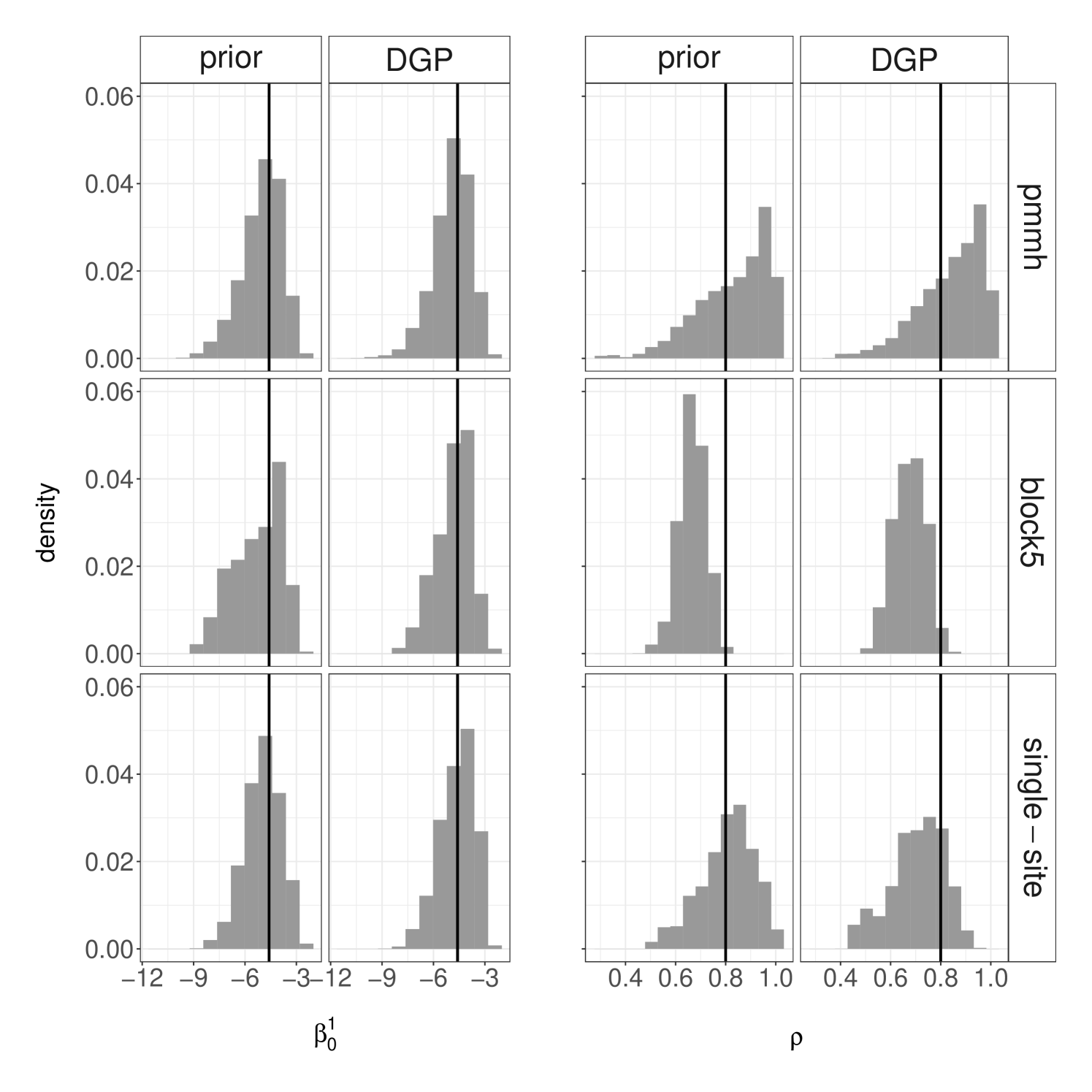
We now describe various MCMC algorithms that can be used to sample from the smoothing distribution pθ(x0:T|y0:T)p_{\theta}(x_{0:T}|y_{0:T}) of the agent-based SIS model in Section 3. These Gibbs sampling strategies can be seen as alternatives to the SMC approach in Sections 3.1 and 3.2. The same ideas can also be applied to the SIR model in Section 4 with some modifications.

A simple option is a single-site update that samples the state of an agent at a specific time from the full conditional distribution pθ(xtn|x0:t1,xtn,xt+1:T,y0:T)p_{\theta}(x_{t}^{n}|x_{0:t-1},x_{t}^{-n},x_{t+1:T},y_{0:T}), where xtn=(xtm)m[1:N]nx_{t}^{-n}=(x_{t}^{m})_{m\in[1:N]\setminus n}, for t[0:T]t\in[0:T] and n[1:N]n\in[1:N] that can be chosen deterministically or randomly with uniform probabilities using a systematic or random Gibbs scan. Using the conditional independence structure of the model, for t[1:T1]t\in[1:T-1], this full conditional is a Bernoulli distribution with success probability that is proportional to

αn(xt1)Bin(yt;I(x~t),ρ)m𝒩(n)Ber(xt+1m;αm(x~t)),\displaystyle\alpha^{n}(x_{t-1})\text{Bin}(y_{t};I(\tilde{x}_{t}),\rho)\prod_{m\in\mathcal{N}(n)}\text{Ber}(x_{t+1}^{m};\alpha^{m}(\tilde{x}_{t})), (106)

where x~t=(xtm)m[1:N]\tilde{x}_{t}=(x_{t}^{m})_{m\in[1:N]} with xtn=1x_{t}^{n}=1. This expression also holds for the case t=0t=0 by replacing αn(xt1)\alpha^{n}(x_{t-1}) with α0n\alpha_{0}^{n}, and t=Tt=T by removing the last product. As each update costs 𝒪(𝒟(n))\mathcal{O}(\mathcal{D}(n)), the overall cost of a Gibbs scan is 𝒪(Tn=1N𝒟(n))\mathcal{O}(T\sum_{n=1}^{N}\mathcal{D}(n)).

As discussed in Ghahramani and Jordan [1996] for a related class of models, one can consider block updates that jointly sample the trajectory of a few agents. For a subset b[1:N]b\subseteq[1:N] of size BB, this Gibbs update involves sampling from pθ(x0:Tb|x0:Tb,y0:T)p_{\theta}(x_{0:T}^{b}|x_{0:T}^{-b},y_{0:T}), where x0:Tb=(xtn)t[0:T],nbx_{0:T}^{b}=(x_{t}^{n})_{t\in[0:T],n\in b} and x0:Tb=(xtn)t[0:T],n[1:N]bx_{0:T}^{-b}=(x_{t}^{n})_{t\in[0:T],n\in[1:N]\setminus b}. This can be done using the forward-backward algorithm in 𝒪((22B+2BN)T)\mathcal{O}((2^{2B}+2^{B}N)T) cost. Hence the overall cost of a systematic Gibbs scan over the entire population is 𝒪((22B+2BN)TN/B)\mathcal{O}((2^{2B}+2^{B}N)TN/B). As the latter is computationally prohibitive for large BB, one has to consider reasonably small block sizes.

We can also employ a swap update that leaves the full conditional distribution pθ(xt|x0:t1,xt+1:T,y0:T)p_{\theta}(x_{t}|x_{0:t-1},x_{t+1:T},y_{0:T}) invariant for each t[0:T]t\in[0:T] (with x0:1=xT+1:T=x_{0:-1}=x_{T+1:T}=\emptyset). Let xtx_{t} denote the current state of the population at time tt. We will choose n0n_{0} and n1n_{1} uniformly from the sets {i:xti=0}\{i:x_{t}^{i}=0\} and {i:xti=1}\{i:x_{t}^{i}=1\} respectively. The proposed state x~t\tilde{x}_{t} is such that x~tn0=1\tilde{x}_{t}^{n_{0}}=1, x~tn1=0\tilde{x}_{t}^{n_{1}}=0 and x~tn=xtn\tilde{x}_{t}^{n}=x_{t}^{n} for n[1:N]{n0,n1}n\in[1:N]\setminus\{n_{0},n_{1}\}. For t[1:T1]t\in[1:T-1], the MH acceptance probability is

min{1,αn0(xt1)(1αn1(xt1))n=1NBer(xt+1n;αn(x~t))αn1(xt1)(1αn0(xt1))n=1NBer(xt+1n;αn(xt))}.\displaystyle\min\left\{1,\frac{\alpha^{n_{0}}(x_{t-1})(1-\alpha^{n_{1}}(x_{t-1}))\prod_{n=1}^{N}\text{Ber}(x_{t+1}^{n};\alpha^{n}(\tilde{x}_{t}))}{\alpha^{n_{1}}(x_{t-1})(1-\alpha^{n_{0}}(x_{t-1}))\prod_{n=1}^{N}\text{Ber}(x_{t+1}^{n};\alpha^{n}(x_{t}))}\right\}. (107)

The case t=0t=0 can be accommodated by replacing α(xt1)\alpha(x_{t-1}) with α0\alpha_{0}, and t=Tt=T by removing the ratios of Bernoulli PMFs. The cost of each swap update ranges between 𝒪(1)\mathcal{O}(1) and 𝒪(N)\mathcal{O}(N), depending on the structure of the network. As swap updates on their own do not change the number of infected agents, we propose to employ them within a mixture kernel that also relies on the above-mentioned forward-backward scans.

As alternatives to PMMH, we can consider Gibbs samplers that alternate between sampling the parameters from p(θ|x0:T,y0:T)p(\theta|x_{0:T},y_{0:T}) using a MH algorithm, and the agent states from pθ(x0:T|y0:T)p_{\theta}(x_{0:T}|y_{0:T}) using the above MCMC algorithms. In particular, we employ an equally weighted mixture of kernels, performing either NN random swap updates for each time step, or systematic Gibbs scan with single-site updates (“single-site”) or block updates for B=5B=5 agents (“block5”). We compare these Gibbs samplers to PMMH on the simulated dataset of Section 3.3. We set the MH Normal proposal standard deviation within Gibbs samplers as 0.080.08 to achieve suitable acceptance probabilities. We initialize the parameters from either the DGP or the prior distribution, and run all algorithms for the same number of iterations. Figure 7 displays the resulting approximations of the marginal posterior distribution of two parameters. Compared to the Gibbs samplers, the PMMH approximations seem to be more stable between runs with different initializations. These plots also suggest that the Gibbs samplers provide a poorer exploration of the tails of the posterior distribution, which may be attributed to the dependence between the agent states and parameters in this setting.

Refer to caption
Figure 7: Histograms illustrating approximations of the marginal posterior distributions of β01\beta_{0}^{1} and ρ\rho, obtaining using PMMH chains and Gibbs samplers with either single-site or block updates, and initialization from either the DGP or the prior distribution. Black vertical lines depict the DGP.