Set-Membership Filtering-Based Leader-Follower Synchronization of Discrete-time Linear Multi-Agent Systems
Abstract
In this paper, a set-membership filtering-based leader-follower synchronization protocol for discrete-time linear multi-agent systems is proposed wherein the aim is to make the agents synchronize with a leader. The agents, governed by identical high-order discrete-time linear dynamics, are subject to unknown-but-bounded input disturbances. In terms of its own state information, each agent only has access to measured outputs that are corrupted with unknown-but-bounded output disturbances. Also, the initial states of the agents are unknown. To deal with all these unknowns (or uncertainties), a set-membership filter (or state estimator), having the ‘correction-prediction’ form of a standard Kalman filter, is formulated. We consider each agent to be equipped with this filter that estimates the state of the agent and consider the agents to be able to share the state estimate information with the neighbors locally. The corrected state estimates of the agents are utilized in the local control law design for synchronization. Under appropriate conditions, the global disagreement error between the agents and the leader is shown to be bounded. An upper bound on the norm of the global disagreement error is calculated and shown to be monotonically decreasing. Finally, two simulation examples are included to illustrate the effectiveness of the proposed set-membership filter and the proposed leader-follower synchronization protocol.
Keywords: Multi-agent systems, cooperative control, synchronization, set-membership filtering, optimization.
1 Introduction
Cooperative control of multi-agent systems can be applied to solve a number of engineering problems and has attracted much attention in the last few decades. The applications of cooperative control include distributed task assignment and consensus problems, formation flight of spacecrafts and aerial vehicles, distributed estimation problems and so on (see, for example, Refs. [1, 2, 3, 4, 5, 6]). All of these applications typically require some degree of cooperation and synchronization among the agents. In the context of synchronization (or consensus), there are several types of problems that have been investigated in the existing literature. These are (a) synchronization without a leader (see, for example, Refs. [7, 8]), (b) leader-follower synchronization (see, for example, Refs. [9, 10, 11, 12]), (c) average consensus (see, for example, Refs. [13, 14]), (d) bipartite consensus (see, for example, Ref. [15]) and so on. In this paper, we focus on leader-follower synchronization in the presence of a leader that pins to a group of agents, all having high-order discrete-time linear (time-invariant) dynamics.
1.1 Motivation
Most of the studies in the existing literature regarding multi-agent synchronization assume perfect modeling of the system, i.e., the mathematical description of the system is assumed to be perfect (see, for example, Refs. [8, 10, 11, 16, 17, 12]). However, this is incompatible with real-world engineering problems where the dynamical system is subject to unknown input disturbances, parametric uncertainties, unmodeled dynamics, etc. Because of these phenomena, the state of the system can not be known precisely and should be considered uncertain. For an overview on synchronization in uncertain multi-agent systems, see Refs. [6, 7, 9, 18] and references therein. Among the abovementioned phenomena, we focus on unknown input disturbances in this paper. Apart from the perfect system modeling assumption, perfect information regarding the states of the agents (full-state feedback) are assumed to be available for synchronization protocol design in a large number of studies (see, for example, Refs. [16, 10, 8]). Again, this assumption does not hold for practical applications where measured outputs (some function of the states), subject to output disturbances, are available. Although observer-based approaches, without considering output disturbances, have been investigated in the literature (see, for example, Refs. [4, 17, 9]), a state estimation or filtering-based approach would be more suitable to address the effects of both input and output disturbances in the synchronization problem (see, for example, Ref. [5]).
The Kalman filter [19], which is one of the most widely-studied stochastic filtering techniques, assumes that the input and output disturbances are Gaussian noises with known statistical properties. However, this assumption is difficult to validate in practice and might not hold for real-world systems. Therefore, it seems more realistic to assume the disturbances to be unknown-but-bounded [20, 21]. This approach leads to the concept of set-membership or set-valued state estimation (or filtering) (see, for example, Refs. [22, 23, 20, 24, 25, 21, 26]), which is deterministic and more suited to several practical applications [24]. Although the set-theoretic or set-valued concepts for synchronization have been investigated in the existing literature (see, for example, Refs. [27, 28, 29, 30]), studies explicitly utilizing set-membership or set-valued estimation techniques for the multi-agent synchronization problem are relatively rare (see, for instance, Refs. [13, 14]), despite the practical significance of this class of estimators/filters. Recently, a leader-follower synchronization protocol using set-membership estimation techniques was put forward in Ref. [31]. The synchronization objective in Ref. [31] was to construct ellipsoids centered at the leader’s state trajectory that contained states of the agents. This, however, is different from the concept of conventional leader-follower synchronization where the objective is to make the states of the agents converge to the leader’s state trajectory. To the best of the authors’ knowledge, set-membership estimation techniques have not been employed for the conventional leader-follower synchronization problem in the existing literature.
1.2 Technical Approach and Contributions
The technical approach and contributions of the paper are summarized in the following list.
-
We develop a set-membership estimation-based (conventional) leader-follower synchronization protocol for high-order discrete-time linear multi-agent systems with the agents subject to unknown-but-bounded input and output disturbances. To the best of our knowledge, this is a novel contribution.
-
Specifically, we focus on the ellipsoidal state estimation problem and adopt the terminology set-membership filter (SMF). Based on the approaches given in Refs. [23, 25, 24, 26], we convert the set estimation problem into a recursive algorithm that requires solutions to two semi-definite programs (SDPs) at each time-step.
-
We consider each agent to be equipped with the SMF that estimates the state of the agent. Further, we assume that the agents are able to share the state estimate information with the neighbors locally and that information is utilized in the local control synthesis for synchronization. The local controller for each agent is chosen based on an type Riccati-based approach [16]. We show that the global error system is input-to-state stable (ISS) with respect to the input disturbances and estimation errors. Sufficient conditions for input-to-state stability are provided in terms of the system matrices of the agents, the Riccati design, and the interaction graph.
-
Further, we calculate an upper bound on the norm of the global disagreement error and show that it decreases monotonically, converging to a limit as time goes to infinity.
The rest of this paper is organized as follows. Section 2 describes the preliminaries required for the SMF design. The formulation of the SMF is given in Section 3. The control input synthesis and related results for synchronization are given in Section 4. Finally, Section 5 includes the simulation examples and Section 6 presents the concluding remarks.
Notations and definitions
The symbol denotes the set of non-negative integers. For a square matrix , the notation (respectively, ) means is symmetric and positive definite (respectively, positive semi-definite). Similarly, (respectively, ) means is symmetric and negative definite (respectively, negative semi-definite). Further, denotes the spectral radius of a square matrix . For any matrix , stands for the maximum singular value of . denotes an open circle of radius in the complex plane, centered at . Notations , , , , and denote block-diagonal matrices, the identity matrix, the null matrix, and the vector of ones and zeros of dimension , respectively. For vectors , we have . The symbol denotes standard Euclidean norm for vectors and induced matrix norm for matrices. For any function , we have . This is the standard norm for a bounded . Ellipsoids are denoted by where is the center of the ellipsoid and is the shape matrix that characterizes the orientation and ‘size’ of the ellipsoid in . Notations , denote trace and rank of a matrix, respectively, and denotes the Kronecker product. The superscript T means vector or matrix transpose.
2 Preliminaries
Consider the discrete-time dynamical systems of the form
| (1) |
where is the state, is the control input, is the input disturbance, is the measured output, is the output disturbance. Also, , , , and are system matrices of appropriate dimensions. Following are the assumptions for systems of the form given in Eq. (1).
Assumption 1
-
1.1
The initial state is unknown. However, it satisfies where is a given initial estimate and is known.
-
1.2
and are unknown-but-bounded for all . Also, and for all where , are known.
We intend to develop an SMF for systems of the form in Eq. (1), having a correction-prediction structure similar to the Kalman filter variants (see, for example, Ref. [19]). Note that the SMF design in this paper is motivated by the SMF developed by the authors in Ref. [34]. The filtering objectives are as follows where the corrected and predicted state estimates at time-step are denoted by and , respectively [34].
2.1 Correction Step
At each time-step , upon receiving the measured output with and given , the objective is to find the optimal correction ellipsoid, characterized by and , such that . The corrected state estimate is given by
| (2) |
where is the filter gain. Since , there exists a with such that
| (3) |
2.2 Prediction Step
At each time-step , given and , the objective is to find the optimal prediction ellipsoid, characterized by and , such that where the predicted state estimate is given by
| (4) |
Again, since , we have
| (5) |
where and . Initialization is provided by and [19].
Remark 1
As mentioned in the filtering objectives, we are interested in finding the optimal ellipsoids, i.e., the minimum-‘size’ ellipsoids, at each time-step. There are two criteria for the ‘size’ of an ellipsoid in terms of its shape matrix: trace criterion and log-determinant criterion [23]. In this paper, we have considered the trace criterion (see Theorems 1 and 3.3) which represents the sum of squared lengths of semi-axes of an ellipsoid [23]. As a result, the corresponding optimization problems are convex (see the SDPs in Eqs. (6) and (15)). Alternatively, for minimum-volume ellipsoids, one can consider the log-determinant criterion. However, this would render the optimization problems non-convex and additional modifications might be required to restore convexity (see, for example, Ref. [23]).
3 Set-Membership Filter Design
In this section, we formulate the SDPs to be solved at each time-step for the SMF. As the SMF design is motivated by the one in [34], we have adopted the notations and relevant statements provided in [34]. First, we state the result that summarizes the filtering problem at the correction step.
Theorem 1
Consider the system in Eq. (1) under the Assumption 1. Then, at each time-step , upon receiving the measured output with and given , the state is contained in the optimal correction ellipsoid given by , if there exist , , as solutions to the following SDP:
| (6) |
where and are given by
| (7) |
Furthermore, the center of the correction ellipsoid is given by the corrected state estimate in Eq. (2).
Proof 3.2.
Using Eqs. (1), (2), and (3), we have
| (8) |
Next, we define . Therefore, Eq. (8) can be expressed in terms of as
| (9) |
where is as shown in Eq. (7). Now, is given by
| (10) |
The unknowns in should satisfy the following inequalities:
| (11) |
which can be expressed in terms of as
| (12) |
Next, the S-procedure (see, for example, Ref. [35]) is applied to the inequalities in Eqs. (10) and (12). Thus, a sufficient condition such that the inequalities given in Eq. (12) imply the inequality in Eq. (10) to hold is that there exist such that the following is true:
The above inequality can be expressed in a compact form as
| (13) |
where is as shown in Eq. (7). Using the Schur complement (see, for example, Ref. [35]), we express the inequality in Eq. (13) equivalently as
| (14) |
Solving the inequality in Eq. (14) with , yields a correction ellipsoid containing the state . Then, the optimal correction ellipsoid is found by minimizing the trace of subject to , , and Eq. (14). This completes the proof. ∎
Next, we state the technical result for the prediction step.
Theorem 3.3.
Consider the system in Eq. (1) under the Assumption 1 with the state in the correction ellipsoid and . Then, the successor state belongs to the optimal prediction ellipsoid , if there exist , as solutions to the following SDP:
| (15) |
where and are given by
Furthermore, the center of the prediction ellipsoid is given by the predicted state estimate in Eq. (4).
Proof 3.4.
Follows directly from the proof of Theorem 1 and has been omitted. ∎
Interior point methods can be implemented to efficiently solve the SDPs in Eqs. (6) and (15) [36]. The recursive SMF algorithm is summarized in Algorithm 1.
4 Leader-Follower Synchronization of Multi-Agent Systems
This section describes local control input synthesis for the leader-follower synchronization. Results presented in this section are based on the results given in Ref. [16] and, to be consistent, we have adopted some of the terminologies and notations used in Ref. [16].
4.1 Graph related preliminaries [1]
Consider a multi-agent system consisting of agents. The communication topology of the multi-agent system can be represented by a graph where is a nonempty node set and is an edge set of ordered pairs of nodes, called edges. Node in the graph represents agent . We consider simple, directed graphs in this paper. The edge in the edge set of a directed graph denotes that node can obtain information from node , but not necessarily vice versa. If an edge , then node is a neighbor of node . The set of neighbors of node is denoted as .
The adjacency matrix of a directed graph is defined such that is a positive weight if , and otherwise. The graph Laplacian matrix is defined as where is the in-degree matrix with , and . A directed path is a sequence of edges in a directed graph of the form (, ), (, ), . The graph contains a (directed) spanning tree if there exists a node, called the root node, such that every other node in can be connected by a directed path starting from that node.
4.2 Synchronization: Formulation and Results
We consider agents connected via a directed graph and a leader. Agent () is a dynamical system of the form
| (16) |
where , , , , are the state, control input, measured output, input and output disturbances for agent , respectively. Clearly, the system described by Eq. (16) is in the form of the system described by Eq. (1), with the time-varying matrices replaced by the constant matrices. Next, we modify Assumption 1 and impose the following assumptions on the dynamics of agent ().
Assumption 2
-
2.1
The initial state is unknown. However, it satisfies where is a given initial estimate and is known. Also, holds with some .
-
2.2
and are unknown-but-bounded for all . Also, and for all where , are known with and for all with some .
Under this assumption, agent () employs the SMF in Algorithm 1 to estimate its own state. Now, we introduce the following assumption on the system matrices of the agents.
Assumption 3
is full column rank with the pair stabilizable.
We consider the leader to be a system of the form
| (17) |
where is the leader’s state and is the output. Note that the leader is a virtual system that generates the reference trajectory for the agents to track. We define the local neighborhood tracking errors, using the corrected state estimates of the agents, as
where are the pinning gains, and are the corrected state estimates of agent and , respectively. If agent is pinned to the leader, we take . Now, we choose the control input of agent as [16]
where is a coupling gain and is a control gain matrix to be discussed subsequently. Hence, the global dynamics of the agents can be expressed as
| (18) |
with , , and
| (19) |
where is the matrix of pinning gains, , and . Note that the superscript is utilized to denote the global variables. Now, using Eq. (5) for each agent’s corrected state estimates, we can express as
| (20) |
where , . Note that where is the correction ellipsoid shape matrix for agent and for . Our next assumption is regarding the interaction graph.
Assumption 4 ([16])
The interaction graph contains a spanning tree with at least one nonzero pinning gain that connects the leader and the root node.
The global disagreement error [16] is defined as . Utilizing Eqs. (18)-(20), we express the global error system as
| (21) |
where
| (22) |
with . Now, we recall the following technical result from Ref. [16].
Lemma 4.5 ([16]).
iff for all the eigenvalues of .
If the matrix is unstable or marginally stable, then Lemma 4.5 requires Assumption 4 with the pair stabilizable [16]. Using Theorem 2 in Ref. [16], and are chosen such that . To this end, we state the following result.
Lemma 4.6 ([16]).
Let Assumption 4 hold and let be a positive definite solution to the discrete-time Riccati-like equation
| (23) |
for some . Define
Further, let there exist a containing all the eigenvalues of such that . Then, for and .
If is full column rank, Eq. (23) has a positive definite solution only if the pair is stabilizable [16]. In this regard, Assumption 3 is pertinent. Next, we introduce the notion of input-to-state stability in the following definition.
Definition 4.7.
A discrete-time system of the form with , , is (globally) input-to-state stable (ISS) if there exist a class function and two class functions such that, for each pair of inputs , and each , it holds that
| (24) |
for each .
Remark 4.8.
We state the main result of this section in the next theorem.
Theorem 4.9.
Proof 4.10.
The proof is inspired by Example 3.4 in Ref. [32]. Let us denote where are the state estimation errors of agent at the correction steps. Now, using Eq. (20), we have . Similarly, let us denote where is the initial estimation error of agent . Due to Assumption 2, we have
| (25) |
with , where and for . Then, Eq. (21) becomes
where are the inputs. It is understood that and . Due to the choices of and along with Assumptions 3 and 4, we have . Hence, there exist constants and such that [32]. Then, the ISS property in Eq. (24) holds for the system in Eq. (21) with
| (26) |
where is utilized. Thus, along the trajectories of the system in Eq. (21), for each , it holds that
| (27) |
where the functions are as in Eq. (26) with , , . This completes the proof. ∎
Theorem 4.9 implies that the global disagreement error remains bounded under the proposed synchronization protocol.
Remark 4.11.
Objective of the SMF-based synchronization in Ref. [31] was to contain the states of the agents in a confidence ellipsoid which might not be small in general. Thus, the approach outlined in Ref. [31] may lead to conservative results where the states of the agents might not converge to a neighborhood of the leader’s state trajectory. On the other hand, we have shown that, under appropriate conditions, the global error system is ISS with respect to the input disturbances and estimation errors. Since an ISS system admits the ‘converging-input converging-state’ property (see, Refs. [32, 37] for details), would eventually converge to a neighborhood of zero as the estimation errors of the agents decrease. Thus, the agents would converge to a neighborhood of the leader’s state trajectory. To this end, it is understood that is relatively small (compared to and ) as the input disturbances satisfy Assumption 2.2.
Corollary 4.12.
Under the conditions of Theorem 4.9, the normalized global disagreement error satisfies
| (28) |
with where and , are such that for all .
Proof 4.13.
Under the conditions of Theorem 4.9, the result in Eq. (27) holds. Then, let us rewrite Eq. (27) as
Now, under the assumption that the SMFs of the agents are performing adequately, we can utilize Eq. (25) and take . Using Assumption 2, we have . Also, we have . Therefore, we derive . Similarly, Assumption 2 leads to . Combining these, we calculate the following bound on
| (29) |
for each with . Hence, the proof is completed by taking the limit in Eq. (28) and carrying out the normalization . ∎
Remark 4.14.
Remark 4.15.
For a given multi-agent system (with the number of agents , the matrices , and the interaction graph specified), we have and fixed once and are properly chosen using Lemma 4.6. Thus, the conservatism of the bound in Eq. (28) can be reduced if the available upper bounds (i.e., and ) are sufficiently small.
5 Simulation Examples
Simulation examples are provided in this section to illustrate the effectiveness of the proposed SMF and SMF-based leader-follower synchronization protocol. All the simulations are carried out on a desktop computer with a 16.00 GB RAM and a 3.40 GHz Intel(R) Xeon(R) E-2124 G processor running MATLAB R2019a. The SDPs in Eqs. (6) and (15) are solved utilizing ‘YALMIP’ [38] with the ‘SDPT3’ solver in the MATLAB framework. Since the disturbances are only assumed to be unknown-but-bounded, different kinds of disturbance realizations are possible that satisfy the ellipsoidal assumptions (Assumptions 1.2 and 2.2). For example, periodic disturbances with time-varying or constant frequencies and amplitudes, random disturbances with each element being uniformly distributed in an interval, and so on.
5.1 Example-1
In this example, we illustrate the effectiveness of the proposed SMF algorithm and compare our results with the results obtained for the SMF in Ref. [39] (the discrete version). We choose a system governed by the Mathieu equation [39] for this example, i.e., the system given by
| (30) |
which is expressed in a compact form as
| (31) |
where
| (32) |
with as the input disturbance. Utilizing zeroth-order hold (ZOH) with a sampling time , the above system is put into an equivalent discrete-time form as
| (33) |
where and is the input disturbance at the current time-step. The measured outputs are considered as .
Thus, we have , . The system parameters, , disturbances, disturbance ellipsoid shape matrices, and initial conditions chosen are as follows:
| (34) |
With the above initial conditions, disturbances and disturbance ellipsoid shape matrices, Assumption 1 is satisfied, and we implement the proposed SMF in Algorithm 1 with . The simulation results are shown in Figs. 1 and 2. The estimation errors and error bounds shown in Fig. 1 are corresponding to the correction steps. Thus, we have . As shown in Fig. 1, the estimation errors remain within the corresponding error bounds for the entire time-horizon considered. Thus, the true state is contained in the correction ellipsoids for the entire time-horizon too. The error bounds are time-varying for this example as the dynamical system considered here is time-varying. Further, the error bounds decrease significantly from the corresponding initial values, evidencing the ongoing optimization process for the SMF. The phase plane plot of the true states and corrected state estimates are shown in Fig. 2. Since the estimation errors are small (as shown in Fig. 1), the true state and corrected state estimate trajectories remain in a close neighborhood of each other. This is depicted in Fig. 2. Also, the zoomed-in plot in Fig. 2 shows that the SMF is able to bring the corrected state estimate in a neighborhood of the true state after the correction step at . This explains the small at compared to the initial error (see the zoomed-in plot in Fig. 1).
| Item | Proposed SMF | Balandin et al. (Ref. [39]) |
|---|---|---|
| 0.0434 | 0.0477 | |
| 0.0002 | 0.0015 | |
| 0.00267 | 0.0028 |
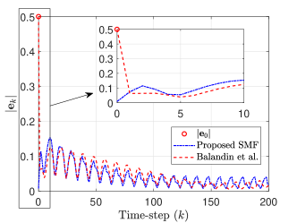
Next, we compare the results of the proposed SMF with the ones corresponding to the SMF framework given in Balandin et al. (Ref. [39], the discrete version). The system parameters, , disturbances, and initial conditons considered for both the frameworks are as shown in Eq. (34). However, the disturbance ellipsoid shape matrices for the framework in Ref. [39] are adopted from the example in section 3 in Ref. [39]. Whereas, for the proposed SMF, the disturbance ellipsoid shape matrices are as shown in Eq. (34). The difference in the disturbance ellipsoid shape matrices are due to the different kinds of ellipsoidal assumptions utilized in this paper, compared to the ones in Ref. [39]. However, these values are chosen such that both sets of disturbance ellipsoid shape matrices are equivalent. The comparison results are shown in Figs. 3, 4. Fig. 3 shows the comparison in estimation error norms where estimation errors at the correction steps for the proposed SMF are depicted. The proposed SMF is able to reduce the error norm at due to the initial correction step (see the zoomed-in plot in Fig. 3). After that, both the SMFs have qualitatively similar error norms. Table 1 illustrates quantitative comparisons of the estimation errors. Clearly, the proposed SMF outperforms the SMF in Ref. [39] in terms of the mean absolute error () and mean squared errors (, ).
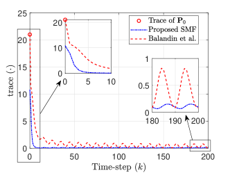
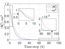
The trace of the shape matrices, corresponding to the correction ellispoids of the proposed SMF and the estimation ellipsoids of the SMF in Ref. [39], are shown in Fig. 4. These results show that overall the correction ellipsoids of the proposed SMF are smaller in ‘size’ compared to the estimation ellipsoids of the SMF in Ref. [39]. Thus, the error bounds shown in Fig. 1 for the proposed SMF are tighter compared to the ones for the SMF in Ref. [39]. Also, the proposed SMF is able to reduce the ‘size’ of the correction ellipsoid at due to the initial correction step, as shown in the zoomed-in plot in Fig. 4. Note that the proposed SMF employs a two-step filtering approach wherein two SDPs are solved during every filter recursion which results in optimal (minimum trace) correction and prediction ellipsoids (with the respective state estimates at the centers). On the other hand, the SMF in Ref. [39] employs a one-step filtering technique with a combined correction and prediction step. Thus, the optimization process for estimation happens only once during each recursion of the SMF in [39]. This is likely the reason for better overall performance of the proposed SMF in this example.
5.2 Example-2
In this example, we illustrate results of the proposed SMF-based leader-follower synchronization protocol. We consider four agents, i.e., . Matrices related to the dynamics of the leader and the agents are
| (35) |
where is marginally stable. Also, Assumption 3 is satisfied with the above choices of and . Ellipsoidal parameters related to the SMFs of the agents are for . The initial state estimates of the agents are as follows: , , , . The true initial state for the agents 1 and 2 (, ) are chosen randomly (uniform distribution) between and . Similarly, the true initial state for the agents 3 and 4 (, ) are chosen randomly (uniform distribution) between and . The input disturbances (, ) are chosen randomly (uniform distribution) between and , and the output disturbances (, ) are chosen randomly (uniform distribution) between and . Thus, Assumption 2 has been satisfied with the above parameters, initial conditions, and disturbance terms. The initial state of the leader is chosen as .
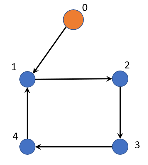
The interaction graph is shown in Fig. 5 and Assumption 4 holds for this interaction graph. Thus, we have
| (36) |
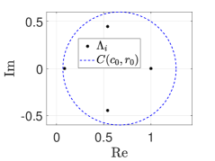
. With regards to Lemma 4.6, we choose , , . Clearly, contains all the eigenvalues of as shown in Fig. 5. Also, we have and . Hence, the conditions for Lemma 4.6 are satisfied and we take , .
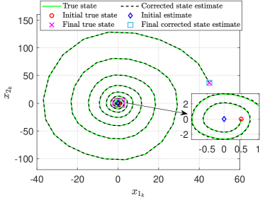
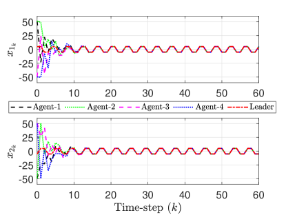
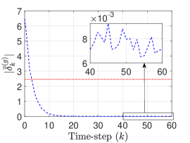
The synchronization results are shown in Figs. 6(a) and 6(b). Figure 6(a) shows that the trajectories of the agents converge close to that of the leader. As a result, the normalized global disagreement error norm converges to a neighborhood of zero (Fig. 6(b)). The red dotted line in Fig. 6(b) denotes the conservative bound in Eq. (28) for which we have utilized and . Also, for , we have taken and . For this choice of and , is satisfied, as shown in Fig. 6(c). With the above values, the conservative upper bound is equal to 2.462, which is shown using the red dotted line in Fig. 6(b).
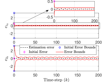
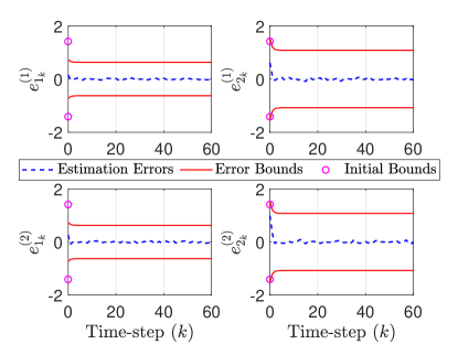
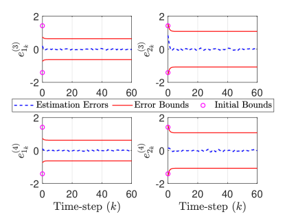
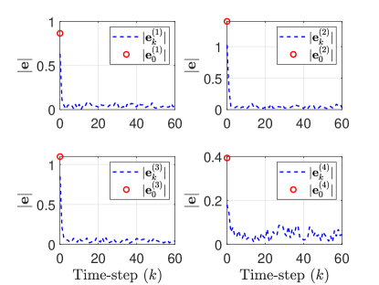
The estimation results corresponding to the SMFs of the agents are shown in Figs. 7, 8, 9, 10. The estimation errors (at the correction steps) for agent ’s SMF are denoted by and the initial errors are denoted by (). Figs. 7, 8 show that the SMFs for the agents perform adequately as the estimation errors remain in a neighborhood of zero and the error bounds decrease from the respective initial values. Also, the estimation errors are contained within the error bounds which mean the SMFs of the agents are able to contain the respective true states inside the respective correction ellipsoids. The estimation error norms, shown in Fig. 9, further illustrate the effectiveness of the SMFs and demonstrate that the SMFs are able to reduce the estimation errors from the respective initial values, starting from the correction step at . The results in Fig. 9 essentially verify our earlier use of in deriving the conservative bound in Eq. (28).
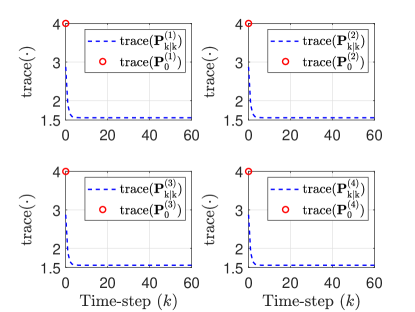
The trace of correction ellipsoid shape matrices for the SMFs of the agents are shown in Fig. 10 where () denote the shape matrices of agent ’s correction ellipsoids. Clearly, SMFs of the agents are able to reduce the trace from the initial values and construct optimal (minimum trace) correction ellipsoids at each time-step (starting from ). Quantitatively, the trace of these shape matrices converge approximately to 1.5 (see Fig. 10), which is approximately a 2.667-fold decrease with respect to the initial trace of 4. The trends shown in Fig. 10 for all the agents are roughly the same as the same set of ellipsoidal parameters is utilized for the SMFs of all the agents and the agents have identical dynamics.
Finally, consider this example with different values of , , , () while keeping all other conditions and parameters unchanged. Now, let us allow for higher magnitudes of disturbances (with , properly chosen such that Assumption 2.2 is satisfied) and compare results with the one given in Fig. 6(b). Results of this study are given in Table 2 where the following two comparison metrics are used: (i) : mean value of ; (ii) : root mean square value of . Also, are chosen randomly (uniform distribution) between and , and are chosen randomly (uniform distribution) between and . Thus, the first row in Table 2 corresponds to the result in Fig. 6(b).
| Disturbance parameters | ||
|---|---|---|
| , | 0.3706 | 1.1985 |
| , | 0.4219 | 1.2052 |
| , | 0.4730 | 1.2124 |
We observe that both the metrics in Table 2 are comparable among the three cases studied, despite the higher magnitudes of disturbances considered for the two cases in second and third rows of Table 2. Therefore, the trends for these two cases with higher disturbance magnitudes would be qualitatively similar to the one shown in Fig. 6(b).
6 Conclusion
A set-membership filtering-based leader-follower synchronization protocol for high-order discrete-time linear multi-agent systems has been put forward for which the global error system is shown to be input-to-state stable with respect to the input disturbances and estimation errors. A monotonically decreasing upper bound on the norm of the global disagreement error vector is calculated. Our future work would involve extending the proposed formulation for discrete-time nonlinear dynamical systems and switching network topologies. Also, we would extend the results in this paper by considering a control input for the leader or the leader to be any bounded reference trajectory. {acknowledgment} This research was supported by the Office of Naval Research under Grant No. N00014-18-1-2215.
References
- [1] Ren, W., and Beard, R. W., 2008. Distributed consensus in multi-vehicle cooperative control. Springer.
- [2] Fax, J. A., and Murray, R. M., 2004. “Information flow and cooperative control of vehicle formations”. IEEE transactions on automatic control, 49(9), pp. 1465–1476.
- [3] Murray, R. M., 2007. “Recent research in cooperative control of multivehicle systems”. ASME Journal of Dynamic Systems, Measurement, and Control, 129(5), pp. 571–583.
- [4] Li, Z., Duan, Z., Chen, G., and Huang, L., 2009. “Consensus of multiagent systems and synchronization of complex networks: A unified viewpoint”. IEEE Transactions on Circuits and Systems I: Regular Papers, 57(1), pp. 213–224.
- [5] Wu, J., Ugrinovskii, V., and Allgöwer, F., 2014. “Cooperative estimation for synchronization of heterogeneous multi-agent systems using relative information”. IFAC Proceedings Volumes, 47(3), pp. 4662–4667.
- [6] Bhusal, R., and Subbarao, K., 2019. “Sensitivity analysis of cooperating multi-agent systems with uncertain connection weights”. In 2019 American Control Conference (ACC), pp. 4024–4029.
- [7] Trentelman, H. L., Takaba, K., and Monshizadeh, N., 2013. “Robust synchronization of uncertain linear multi-agent systems”. IEEE Transactions on Automatic Control, 58(6), pp. 1511–1523.
- [8] Wang, X., Zhu, J., and Cheng, Z., 2015. “Synchronization reachable topology and synchronization of discrete-time linear multi-agent systems”. IEEE Transactions on Automatic Control, 60(7), pp. 1927–1932.
- [9] Back, J., and Kim, J.-S., 2017. “Output feedback practical coordinated tracking of uncertain heterogeneous multi-agent systems under switching network topology”. IEEE Transactions on Automatic Control, 62(12), pp. 6399–6406.
- [10] Li, Z., Wen, G., Duan, Z., and Ren, W., 2014. “Designing fully distributed consensus protocols for linear multi-agent systems with directed graphs”. IEEE Transactions on Automatic Control, 60(4), pp. 1152–1157.
- [11] Lewis, F. L., Cui, B., Ma, T., Song, Y., and Zhao, C., 2016. “Heterogeneous multi-agent systems: reduced-order synchronization and geometry”. IEEE Transactions on Automatic Control, 61(5), pp. 1391–1396.
- [12] Arabi, E., Yucelen, T., and Haddad, W. M., 2017. “Mitigating the effects of sensor uncertainties in networked multi-agent systems”. ASME Journal of Dynamic Systems, Measurement, and Control, 139(4).
- [13] Silvestre, D., Rosa, P., Cunha, R., Hespanha, J. P., and Silvestre, C., 2013. “Gossip average consensus in a byzantine environment using stochastic set-valued observers”. In 52nd IEEE conference on decision and control, IEEE, pp. 4373–4378.
- [14] Silvestre, D., Rosa, P., Hespanha, J. P., and Silvestre, C., 2014. “Finite-time average consensus in a byzantine environment using set-valued observers”. In 2014 American Control Conference, IEEE, pp. 3023–3028.
- [15] Valcher, M. E., and Misra, P., 2014. “On the consensus and bipartite consensus in high-order multi-agent dynamical systems with antagonistic interactions”. Systems & Control Letters, 66, pp. 94–103.
- [16] Hengster-Movric, K., You, K., Lewis, F. L., and Xie, L., 2013. “Synchronization of discrete-time multi-agent systems on graphs using Riccati design”. Automatica, 49(2), pp. 414–423.
- [17] Zhang, H., Lewis, F. L., and Das, A., 2011. “Optimal design for synchronization of cooperative systems: state feedback, observer and output feedback”. IEEE Transactions on Automatic Control, 56(8), pp. 1948–1952.
- [18] Peng, Z., Wang, D., Zhang, H., Sun, G., and Wang, H., 2013. “Distributed model reference adaptive control for cooperative tracking of uncertain dynamical multi-agent systems”. IET Control Theory & Applications, 7(8), pp. 1079–1087.
- [19] Anderson, B. D., and Moore, J. B., 1979. Optimal filtering. Prentice Hall, Inc.
- [20] Polyak, B. T., Nazin, S. A., Durieu, C., and Walter, E., 2004. “Ellipsoidal parameter or state estimation under model uncertainty”. Automatica, 40(7), pp. 1171–1179.
- [21] Chabane, S. B., Maniu, C. S., Alamo, T., Camacho, E. F., and Dumur, D., 2014. “A new approach for guaranteed ellipsoidal state estimation”. IFAC Proceedings Volumes, 47(3), pp. 6533–6538.
- [22] Shamma, J. S., and Tu, K.-Y., 1997. “Approximate set-valued observers for nonlinear systems”. IEEE Transactions on Automatic Control, 42(5), pp. 648–658.
- [23] El Ghaoui, L., and Calafiore, G., 2001. “Robust filtering for discrete-time systems with bounded noise and parametric uncertainty”. IEEE Transactions on Automatic Control, 46(7), pp. 1084–1089.
- [24] Yang, F., and Li, Y., 2009. “Set-membership filtering for discrete-time systems with nonlinear equality constraints”. IEEE Transactions on Automatic Control, 54(10), pp. 2480–2486.
- [25] Yang, F., and Li, Y., 2009. “Set-membership filtering for systems with sensor saturation”. Automatica, 45(8), pp. 1896–1902.
- [26] Wei, G., Liu, S., Song, Y., and Liu, Y., 2015. “Probability-guaranteed set-membership filtering for systems with incomplete measurements”. Automatica, 60, pp. 12–16.
- [27] Xiao, F., and Wang, L., 2012. “Asynchronous rendezvous analysis via set-valued consensus theory”. SIAM Journal on Control and Optimization, 50(1), pp. 196–221.
- [28] Munz, U., Papachristodoulou, A., and Allgower, F., 2011. “Delay robustness in non-identical multi-agent systems”. IEEE Transactions on Automatic Control, 57(6), pp. 1597–1603.
- [29] Garulli, A., and Giannitrapani, A., 2011. “Analysis of consensus protocols with bounded measurement errors”. Systems & Control Letters, 60(1), pp. 44–52.
- [30] Sadikhov, T., Haddad, W. M., Yucelen, T., and Goebel, R., 2017. “Approximate consensus of multiagent systems with inaccurate sensor measurements”. ASME Journal of Dynamic Systems, Measurement, and Control, 139(9).
- [31] Ge, X., Han, Q.-L., and Yang, F., 2016. “Event-based set-membership leader-following consensus of networked multi-agent systems subject to limited communication resources and unknown-but-bounded noise”. IEEE Transactions on Industrial Electronics, 64(6), pp. 5045–5054.
- [32] Jiang, Z.-P., and Wang, Y., 2001. “Input-to-state stability for discrete-time nonlinear systems”. Automatica, 37(6), pp. 857–869.
- [33] Lazar, M., Heemels, W. P. M. H., and Teel, A. R., 2013. “Further input-to-state stability subtleties for discrete-time systems”. IEEE Transactions on Automatic Control, 58(6), June, pp. 1609–1613.
- [34] Bhattacharjee, D., and Subbarao, K., 2020, arXiv:2001.06562v2. “Set-membership filter for discrete-time nonlinear systems using state dependent coefficient parameterization”.
- [35] Boyd, S., El Ghaoui, L., Feron, E., and Balakrishnan, V., 1994. Linear matrix inequalities in system and control theory, Vol. 15. Siam.
- [36] Vandenberghe, L., and Boyd, S., 1996. “Semidefinite programming”. SIAM review, 38(1), pp. 49–95.
- [37] Sontag, E. D., 2003. “A remark on the converging-input converging-state property”. IEEE Transactions on Automatic Control, 48(2), pp. 313–314.
- [38] Löfberg, J., 2004. “Yalmip: A toolbox for modeling and optimization in matlab”. In Proceedings of the CACSD Conference, Vol. 3, Taipei, Taiwan.
- [39] Balandin, D. V., Biryukov, R. S., and Kogan, M. M., 2020. “Ellipsoidal reachable sets of linear time-varying continuous and discrete systems in control and estimation problems”. Automatica, 116, p. 108926.