Shadow Generation with Decomposed Mask Prediction and Attentive Shadow Filling
Abstract
Image composition refers to inserting a foreground object into a background image to obtain a composite image. In this work, we focus on generating plausible shadows for the inserted foreground object to make the composite image more realistic. To supplement the existing small-scale dataset, we create a large-scale dataset called RdSOBA with rendering techniques. Moreover, we design a two-stage network named DMASNet with decomposed mask prediction and attentive shadow filling. Specifically, in the first stage, we decompose shadow mask prediction into box prediction and shape prediction. In the second stage, we attend to reference background shadow pixels to fill the foreground shadow. Abundant experiments prove that our DMASNet achieves better visual effects and generalizes well to real composite images.
1 Introduction
Image composition refers to cutting out a foreground object and pasting it on another background image to acquire a composite image, which could benefit plenty of applications in art, movie, and daily photography (Chen and Kae 2019; Weng et al. 2020; Zhang et al. 2020c). However, the quality of composite images could be significantly compromised by the inconsistency between foreground and background, including appearance, geometric, and semantic inconsistencies. In recent years, many deep learning models (Lin et al. 2018; van Steenkiste et al. 2020; Azadi et al. 2020) have endeavored to tackle different types of inconsistencies in composite images, but only a few works (Hong, Niu, and Zhang 2022) focused on the shadow inconsistency, which is a crucial aspect of appearance inconsistency. In this work, we aim to cope with the shadow inconsistency, i.e., generating plausible shadow for the foreground object to make the composite image more realistic.
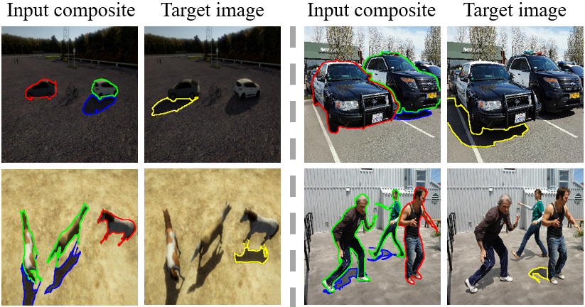
For the shadow generation task, the used data are exhibited in Figure 1. Given a composite image without foreground shadow, the foreground object mask , and the masks of background object-shadow pairs , our goal is generating with foreground shadow. To solve this problem, SGRNet (Hong, Niu, and Zhang 2022) released the first synthetic dataset DESOBA for real-world scenes. The data in DESOBA can be summarized as tuples of the form . The way to obtain pairs in DESOBA is as follows. First, they manually remove the shadows in real images to get shadow-free images. Then, they replace one foreground shadow region in a real image (ground-truth image) with the counterpart in its shadow-free version, yielding a synthetic composite image without foreground shadow. Due to the high cost of manual shadow removal, the scale of DESOBA dataset is very limited (e.g., 1012 ground-truth images and 3623 tuples). Nevertheless, deep learning models require abundant training data.
To supplement DESOBA dataset, we create a large-scale dataset RdSOBA using rendering techniques. We first collect lots of 3D objects and 3D scenes, then place a group of 3D objects in the 3D scene. By using rendering techniques, we can get the images without object shadows and the images with object shadows without manual effort. Finally, we obtain 114,350 ground-truth images and 280,000 tuples. The details of dataset construction can be found in Section 3. Our main goal is using both synthetic dataset DESOBA and rendered dataset RdSOBA to train a model, which can generate foreground shadows for real composite images.
Early shadow generation methods (Zhan et al. 2020; Liu et al. 2020) usually produce terrible results. SGRNet (Hong, Niu, and Zhang 2022) can achieve good metrics on the DESOBA test set, but the generated images have unsatisfactory visual effects and cannot generalize well to real composite images. Specifically, the generated shadows of SGRNet are prone to have notable artifacts like undesired holes and isolated fragments. We also find that SGRNet could not significantly improve the visual effects on both DESOBA and real composite images with the help of our RdSOBA dataset.
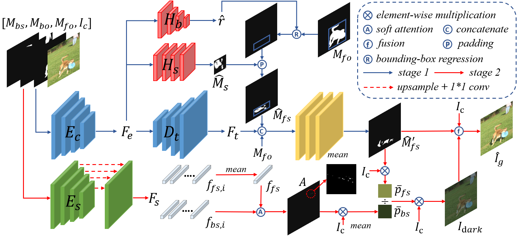
In this work, as illustrated in Figure 2, we design a two-stage network called DMASNet with decomposed mask prediction and attentive shadow filling. In the mask prediction stage, we decompose mask prediction into two sub-tasks: box prediction and shape prediction. Through this decomposition, the first (resp., second) sub-task focuses on predicting the scale/location (resp., shape) of foreground shadow. We first employ a CNN backbone to extract feature from the composite image and a set of masks, then use box head to predict the bounding box of the foreground shadow and shape head to predict the mask shape within the bounding box. After that, the predicted mask shape is placed in the predicted bounding box to produce a rough mask. Then, we concatenate the rough mask with the up-sampled feature map to produce a refined mask. With this structure, the predicted bounding box constrains the range of shadow to suppress isolated fragments and the shape head can generate more solid shadow by concentrating on learning the shapes of real shadows.
In the shadow filling stage, with the observation that the values of foreground shadow pixels are usually close to partial background shadow pixels, we tend to borrow relevant information from background shadow pixels. Based on multi-scale features extracted by a CNN encoder, we calculate the similarities between the average feature within foreground shadow region and pixel-wise background shadow features, resulting in an attention map within background shadow region. Then, we calculate the weighted average of background shadow pixels as the target mean value of foreground shadow pixels. Finally, we scale the pixel values within foreground shadow region to match the target mean value. This strategy makes the generated foreground shadow look compatible with background shadows.
By treating synthetic dataset DESOBA, rendered dataset RdSOBA, and real composite images as three different domains, we also observe that our DMASNet has excellent transferability across different domains. With the assistance of our RdSOBA dataset, our DMASNet can achieve better visual effects than previous methods on DESOBA test set and real composite images. To sum up, our main contributions are as follows,
-
•
We contribute a large-scale rendered dataset RdSOBA for the shadow generation task.
-
•
We propose a novel network DMASNet with decomposed mask prediction and attentive shadow filling.
-
•
Extensive experiments demonstrate that our method achieves better visual effects and generalizes well to real composite images.
2 Related Work
2.1 Image Composition
Image composition refers to cutting out a foreground object from one image and pasting it on another background image to get a composite image. The issues that make the obtained composite images unrealistic can be summarized as appearance, geometry, and semantic inconsistencies (Niu et al. 2021). Lots of works are devoted to solving one or more types of inconsistencies. For instance, object placement methods (Zhang et al. 2020b; Liu et al. 2021; Lee et al. 2018) solved the geometric inconsistency and semantic inconsistency by adjusting the scale, location, and shape of the foreground object. To address the appearance inconsistency, image harmonization methods (Cong et al. 2022; Guo et al. 2021; Ling et al. 2021) adjusted the illumination statistics of foreground, while image blending methods (Zhang et al. 2021; Zhang, Wen, and Shi 2020; Wu et al. 2019) attempted to blend the foreground and background seamlessly. In this work, we target at the missing foreground shadow, which also belongs to appearance inconsistency.
2.2 Shadow Generation
Although there are lots of works on shadow detection (Ding et al. 2019; Chen et al. 2020; Wang et al. 2021) and removal (Zhang et al. 2020a; Le and Samaras 2020; Zhu et al. 2022; Guo et al. 2023), there are few works on shadow generation. Existing works on shadow generation can be divided into two groups according to their adopted technical routes: rendering based methods and image translation methods.
Rendering based methods: Rendering based methods use rendering techniques to generate shadow for the foreground object, during which the 3D information of foreground object and background scene are required. With necessary 3D information, some methods (Karsch et al. 2014; Kee, O’brien, and Farid 2014) obtained the illumination information by interacting with users, while other methods (Liao et al. 2019; Zhang et al. 2019) resorted to traditional algorithms or deep learning networks to predict additional information for a single image. Obviously, the missing information beyond a 2D image is often unavailable and hard to estimate in the real world, so the rendering based methods are difficult to use in practice.
Image translation methods: Deep image-to-image translation methods have become prevalent in recent years. The translation network translates a composite image without foreground shadow to a target image with foreground shadow, which can be categorized into unsupervised methods and supervised methods. Unsupervised methods like (Zhan et al. 2020) mainly use adversarial learning to generate realistic shadows which are indistinguishable from real shadows. Supervised methods have ground-truth images with foreground shadows as supervision. Zhang, Liang, and Wang (2019) exploited a local discriminator to finetune the details and a global discriminator to finetune the global view. Liu et al. (2020) proposed to locate object-shadow pairs in the background to help generate the foreground shadow. Sheng, Zhang, and Benes (2021) predicts the ambient occlusion maps first, then uses a encoder-decoder with the help of the light map manually provided by users to generate soft shadows for the foreground object in simple backgrounds. Hong, Niu, and Zhang (2022) designed cross-attention between foreground encoder and background encoder to predict the mask of foreground shadow, followed by filling the shadow region using predicted shadow parameters.
In this work, we propose novel decompose mask prediction and attentive shadow filling to achieve better transferability and better visual effects.
3 Our RdSOBA Dataset
In this section, we will introduce the details of constructing our RdSOBA dataset.
3.1 Constructing 3D Scenes
We use Unity-3D to construct 3D scenes and render images. There are abundant freely available 3D models and 3D scenes online. We collect 800 standard 3D objects from different categories (e.g., people, vehicles, plants, animals) from CG websites, and 30 representative 3D scenes (e.g., schools, streets, grass) from Unity Asset Store and CG websites. The collected 3D objects and 3D scenes cover a wide range of 3D geometry and object/scene categories, which lays the foundation for generating diverse rendered images.
For each 3D scene, we select 20 open areas to place 3D objects, then choose 10 suitable camera settings (e.g., camera position and viewpoint) for each area. After fixing the camera, we place a group of 3D objects (randomly select 1 to 5 objects from collected 800 objects) in the field of view of camera. For each camera setting, we place 10 groups of 3D objects. With the camera and objects ready, we choose 5 different illumination conditions (e.g., illumination direction, intensity) and render a set of 2D images. Therefore, we can render sets of images.
3.2 Rendering 2D Images
Once we set up an open area, camera settings, 3D object group, and lighting in a 3D scene, we generate a series of images. First, we render an image before placing objects. After placing a group of 3D objects, we switch off the visibility of all objects to the camera and switch on the visibility of each object one by one. When switching on the visibility of the -th object, we can choose whether to render shadow for this object in Unity-3D. Without the shadow, we render an image with the -th object. With the shadow, we render an image with the -th object and its shadow. Based on and , we can obtain the -th object mask by calculating their difference. Similarly, based on and , we can obtain the -th shadow mask . At last, we switch on the visibility of all objects and render an image with the shadows of all objects.
Among 3D objects, when we choose the -th object as the foreground object, we can use (resp., ) as the foreground object (resp., shadow) mask (resp., ). We can merge as the background object mask . Similarly, we can get the background shadow mask . Then, we calculate by , in which denotes element-wise multiplication. Up to now, we have obtained data tuples whose form is identical to DESOBA’s. However, not all the tuples are of high quality because some shadow masks are incomplete or erroneous. After manually filtering out low-quality tuples, we have 280,000 tuples left. We have shown some examples in Figure 1 and more examples can be found in Supplementary.
Although our dataset construction requires certain manual efforts, it is still much more efficient than manually removing the shadows when constructing DESOBA dataset.
4 Our Method
Given an input composite image , the foreground object mask , and the masks of background object-shadow pairs , our DMASNet aims at generating with foreground shadow. We solve this problem with two independent stages: mask prediction stage and shadow filling stage. In the mask prediction stage, we decompose mask prediction into box prediction and shape prediction. The predicted mask shape is placed within the predicted bounding box to form the shadow mask , further refined as . In the shadow filling stage, we predict the target mean value of foreground shadow pixels by attending to relevant background shadow pixels. After filling the predicted shadow mask to match the target mean value, we get the result .
4.1 Decomposed Mask Prediction
In the first stage, our goal is to predict the foreground shadow mask . We use a CNN encoder to extract the bottleneck feature map with size from the concatenation of with size .
Based on , we predict the mask shape and bounding box separately, similar to instance segmentation method Mask-RCNN (He et al. 2017). Unlike instance segmentation where the instance already exists in the input image, we need to imagine the shadow’s shape and bounding box, which is much more challenging than instance segmentation.
Intuitively, by observing background object-shadow pairs, we can roughly estimate the relative scale and location offset of shadow compared with the inserted object. Therefore, we predict the regression from the bounding box of foreground object to that of foreground shadow. We use a quadruplet to describe a bounding box, where are the center coordinates of the bounding box and (resp., ) is the width (resp., height) of the bounding box. The bounding box of foreground object is denoted as and the ground-truth bounding box of foreground shadow is denoted as . Then, we use another quadruplet to characterize the regression from to :
| (5) |
We use box head to predict quadruplet , then calculate the predicted by Eqn. 5. The aspect ratio and position may change significantly when mapping the object bounding box to the shadow bounding box. To consider the coordinate correlation and enhance the robustness, we employ CIoU loss (Zheng et al. 2020) to supervise :
| (6) |
For shape prediction, we do not consider position and aspect ratio handled in , so we generate shape mask within a standardized box for each shadow. For images with size , the mean size of shadow bounding boxes is close to , so we use the shape head to predict a mask with size . We use to denote the operation of cropping the bounding box from image and resizing it to . Inversely, denotes the operation of placing the resized within the bounding box and padding zeros outside the bounding box. In the training phase, the ground-truth shape mask can be obtained by . We calculate loss between and :
| (7) |
After obtaining and , we can get a rough shadow mask by . has roughly correct location, scale, and shape, but lacks fine-grained details. To compensate for detailed information, we employ a decoder , which takes in the bottleneck feature map to produce the up-sampled feature map . Then, is concatenated with and passed through several convolutions layers to yield the refined mask . Again, we use L1 loss to supervise :
| (8) |
4.2 Attentive Shadow Filling
In the second stage, we aim to fill the predicted foreground shadow region. To guarantee that the filled foreground shadow looks compatible with background shadows, one naive approach is calculating the mean value of background shadow pixels as the target mean value of foreground shadow pixels. However, the values of background shadow pixels vary widely and the provided background shadow masks are not perfectly accurate. Hence, we attempt to select reference background shadow pixels by learning different weights for different background shadow pixels.
We apply another encoder to the concatenation of , and concatenate multi-scale encoder features as . Then we average the pixel-wise feature vectors within as . Besides, we denote the pixel-wise feature vector for the -th background shadow pixel as . After that, we project and to a common space via a fully-connected layer and calculate their similarities to produce the attention map , in which is the number of background shadow pixels and . Finally, we calculate the weighted average of background shadow pixels as , in which is the color value of the -th background shadow pixel.
Then, we calculate the average of pixel values within the predicted foreground shadow region as . To match the target mean value , we can get the scale for the foreground shadow region. In implementation, we scale the whole composite image by and obtain the target image by
| (9) |
We employ shadow-MSE loss to supervise the shadow color for the predicted target image:
| (10) |
The whole network can be trained in an end-to-end manner, and the overall loss function can be written as
| (11) |
5 Experiments
5.1 Datasets and Implementation Details
Our RdSOBA dataset has 280,000 training tuples. DESOBA dataset has 2792 training tuples and 580 testing tuples. All images are resized to . We implement our model using PyTorch and train our model on 4*RTX 3090 with batch size being 16. We use the Adam optimizer with the learning rate being 0.0001 and set to (0.5,0.999). We train RENOS for 50 epochs and DESOBA for 1000 epochs without using data augmentation. Further details of our network can be found in the Supplementary.
5.2 Baselines
Following (Hong, Niu, and Zhang 2022), we pick Pix2Pix (Isola et al. 2017), Pix2Pix-Res, Mask-ShadowGAN (Hu et al. 2019), ShadowGAN (Zhang, Liang, and Wang 2019), ARShadowGAN (Liu et al. 2020), and SGRNet (Hong, Niu, and Zhang 2022) as baselines. Pix2Pix is a typical image-to-image translation method. Pix2Pix-Res is a simple variant of Pix2Pix. Mask-ShadowGAN performs shadow removal and mask-guided shadow generation simultaneously, in which the shadow generation network can be adapted to our task. ShadowGAN, ARShadowGAN, and SGRNet work on the same task as ours and thus can be directly applied.
5.3 Evaluation Metrics
| Method | RMSE | S-RMSE | PSNR | S-PSNR |
|---|---|---|---|---|
| Pix2Pix | 7.659 | 75.346 | 31.791 | 6.785 |
| Pix2Pix-Res | 5.961 | 76.046 | 35.073 | 6.678 |
| ShadowGAN | 5.985 | 78.413 | 35.391 | 6.337 |
| Mask-SG | 8.287 | 79.212 | 30.991 | 6.280 |
| AR-SG | 6.481 | 75.099 | 33.720 | 6.790 |
| SGRNet | 4.754 | 61.762 | 37.126 | 8.501 |
| DMASNet | 5.583 | 65.847 | 36.013 | 8.029 |
| Training-set | Method | RMSE | S-RMSE | PSNR | S-PSNR | BER | S-BER | d_hole | d_frag |
|---|---|---|---|---|---|---|---|---|---|
| RdSOBA | SGRNet | 8.127 | 66.603 | 31.025 | 8.033 | 39.220 | 78.137 | 1.024 | 30.686 |
| DMASNet | 7.119 | 63.693 | 33.637 | 8.347 | 28.726 | 57.046 | 0.362 | 10.619 | |
| DESOBA | SGRNet | 4.754 | 61.762 | 37.126 | 8.501 | 26.624 | 53.407 | 15.797 | 100.440 |
| DMASNet | 5.583 | 65.847 | 36.013 | 8.029 | 29.792 | 59.264 | 2.218 | 31.473 | |
| RdSOBA+DESOBA | SGRNet | 4.676 | 59.855 | 36.898 | 8.921 | 27.233 | 54.300 | 5.276 | 56.995 |
| DMASNet | 4.703 | 55.168 | 37.149 | 9.521 | 24.295 | 48.336 | 0.212 | 11.924 |
For comprehensive comparison, we adopt three groups of evaluation metrics.
The first group of metrics are calculated between the ground-truth and the predicted images. We adopt RMSE (resp., shadow-RMSE) and PSNR (resp., shadow-PSNR), that computed on the whole image (resp., ground-truth foreground shadow region). These metrics are valuable, but may not conform to human perception of visual quality.
The second group of metrics are calculated between the ground-truth masks and the predicted masks. We adopt balanced error rate (BER) (resp., shadow-BER), which is computed based on the whole image (resp., ground-truth foreground shadow region). We observe that BER is relatively more consistent with human perception of visual quality.
In the third group, considering that undesired holes and isolated fragments seriously affect human perception without significantly affecting the abovementioned metrics , we design two heuristic metrics to measure the quality of predicted masks. In particular, we calculate the difference between the original mask and that after filling the holes (resp., removing isolated fragments) using the functions in skimage.morphology111remove_small_objects and remove_small_holes. We set connectivity=2 and area_threshold=50, which is referred to d_hole (resp., d_frag). To judge the quality of predicted masks, we should refer to the values of d_hole and d_frag of ground-truth masks.
5.4 Experiments Without Using RdSOBA Dataset
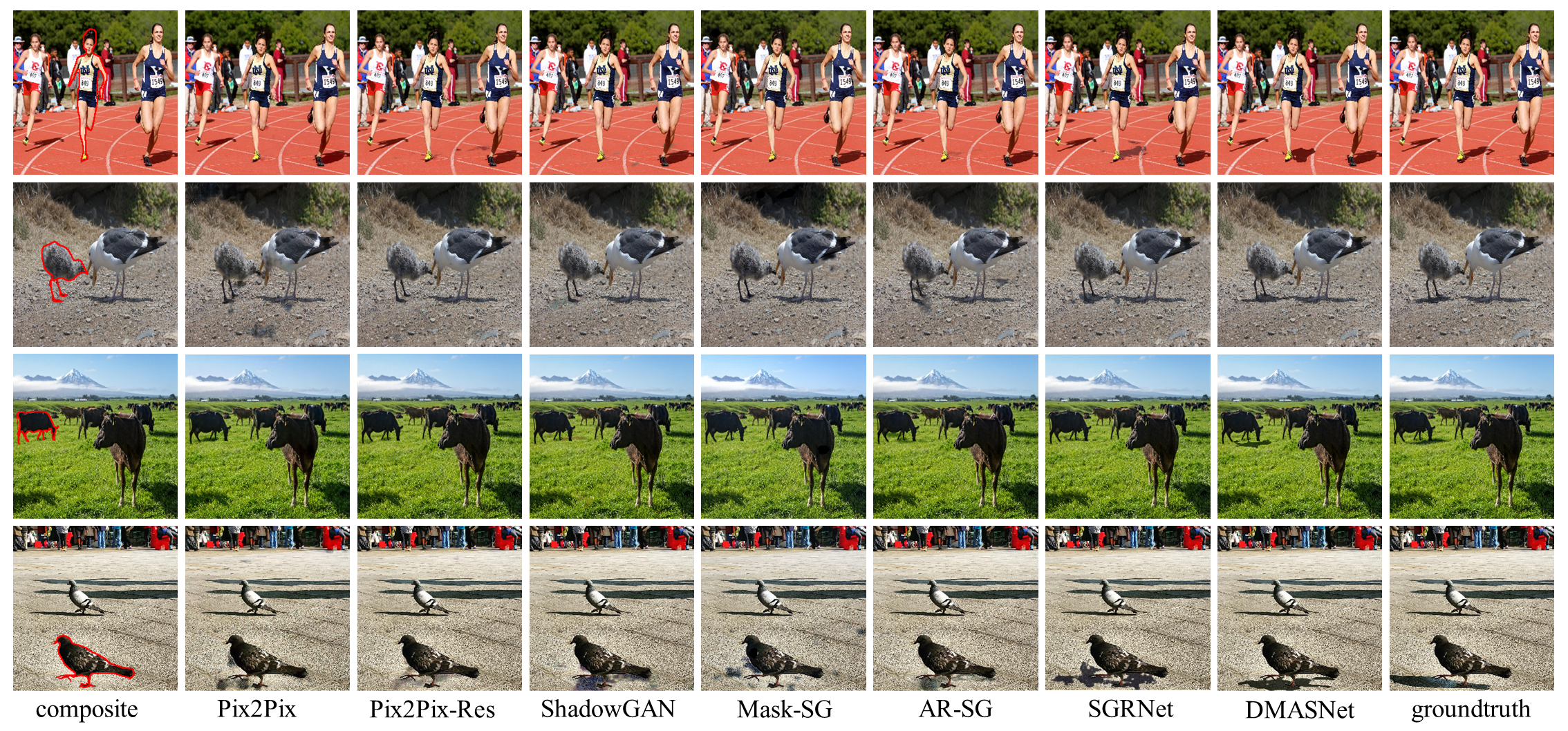
In this section, we only train and evaluate different methods on DESOBA dataset. We show the qualitative results in in Figure 3 and report the quantitative results in Table 1. Since some baselines do not predict the foreground shadow mask, we only calculate the metrics in the first group.
As shown in Figure 3, only our DMASNet and SGRNet can generate plausible shadows, while other methods usually generate terrible shadows. For the quantitative results in Table 1, although our DMASNet is worse than SGRNet on these metrics, the quality of generated images by our DMASNet is comparable with or better than SGRNet. For example, our DMASNet can generate shadows with more compact shapes (e.g., row 4) or more proper intensity values (e.g., row 1). The mismatch between quantitative evaluation and qualitative evaluation motivates us to include more metrics for more comprehensive comparison.
5.5 Experiments Using RdSOBA Dataset
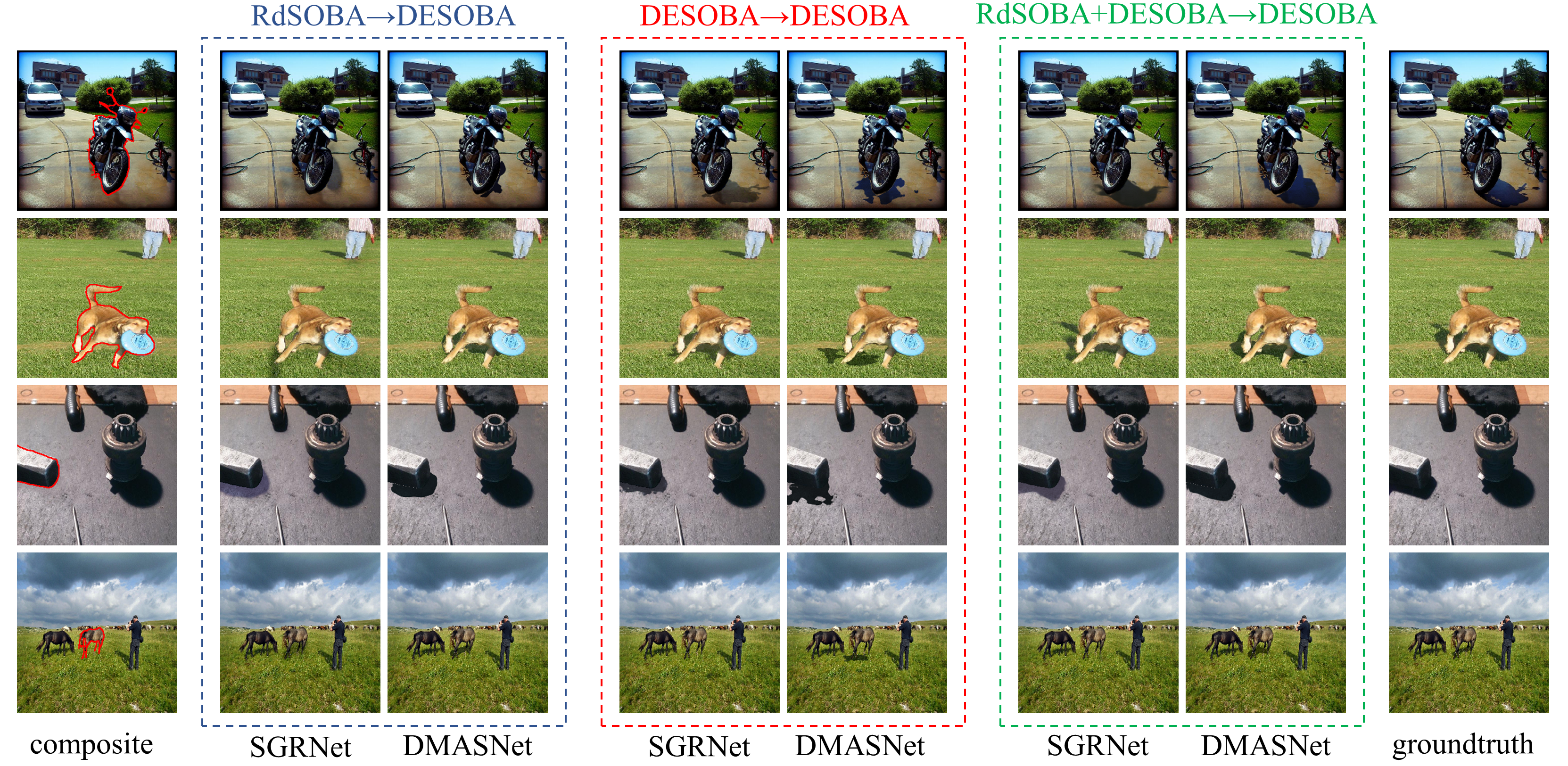
In this section, we only compare with SGRNet because the performances of other baselines are poor as demonstrated in Section 5.4. We conduct experiments in three settings: 1) only using RdSOBA training set; 2) only using DESOBA training set; 3) using both RdSOBA training set and DESOBA training set (first training on RdSOBA, then finetune on DESOBA). For all settings, the evaluation is performed on DESOBA test set. The full comparisons between DMASNet and SGRNet in three settings are summarized in Table 2. We show the advantages of our method from three aspects.
Evaluation metrics: With the help of our RdSOBA, our DMASNet demonstrates notable superiority over SGRNet in metrics. Nevertheless, our RMSE and PSNR remains comparable to SGRNet’s. One reason is that our DMASNet is more likely to produce more shadows than SGRNet, so the MSE of those false positive pixels (non-shadow pixels that are wrongly predicted as shadow pixels) is larger. When using DESOBA or RdSOBA+DESOBA as training set, compared with SGRNet, the d_hole and d_frag of our DMASNet are also closer to those of ground-truth masks.
Cross-domain transferability: When using RdSOBA as training set, the results of SGRNet are poor (row 1). In contrast, the results of DMASNet are even better than those obtained by using DESOBA training set (row 2 v.s. row 4). The contrasting behaviors of SGRNet and our DMASNet show the gap between their transferability. Moreover, with RdSOBA, DMASNet can achieve much better results (row 6 v.s. row 4), but the improvement of SGRNet is marginal (row 5 v.s. row 3), which also demonstrates that our DMASNet has better transferability across different domains.
Visual effects: As shown in Figure 4, the results of DMASNet are substantially improved with the aid of RdSOBA, which are more realistic and closer to the ground-truth images. However, the improvement of SGRNet is not apparent.
| Training-set | Method | B-T score | d_hole | d_frag |
|---|---|---|---|---|
| DESOBA | Pix2Pix-Res | -1.149 | - | - |
| ShadowGAN | -1.206 | - | - | |
| SGRNet | -0.104 | 21.540 | 200.430 | |
| DMASNet | 0.648 | 2.630 | 67.300 | |
| RdSOBA+ DESOBA | SGRNet | -0.192 | 5.460 | 124.050 |
| DMASNet | 2.039 | 1.440 | 18.930 |
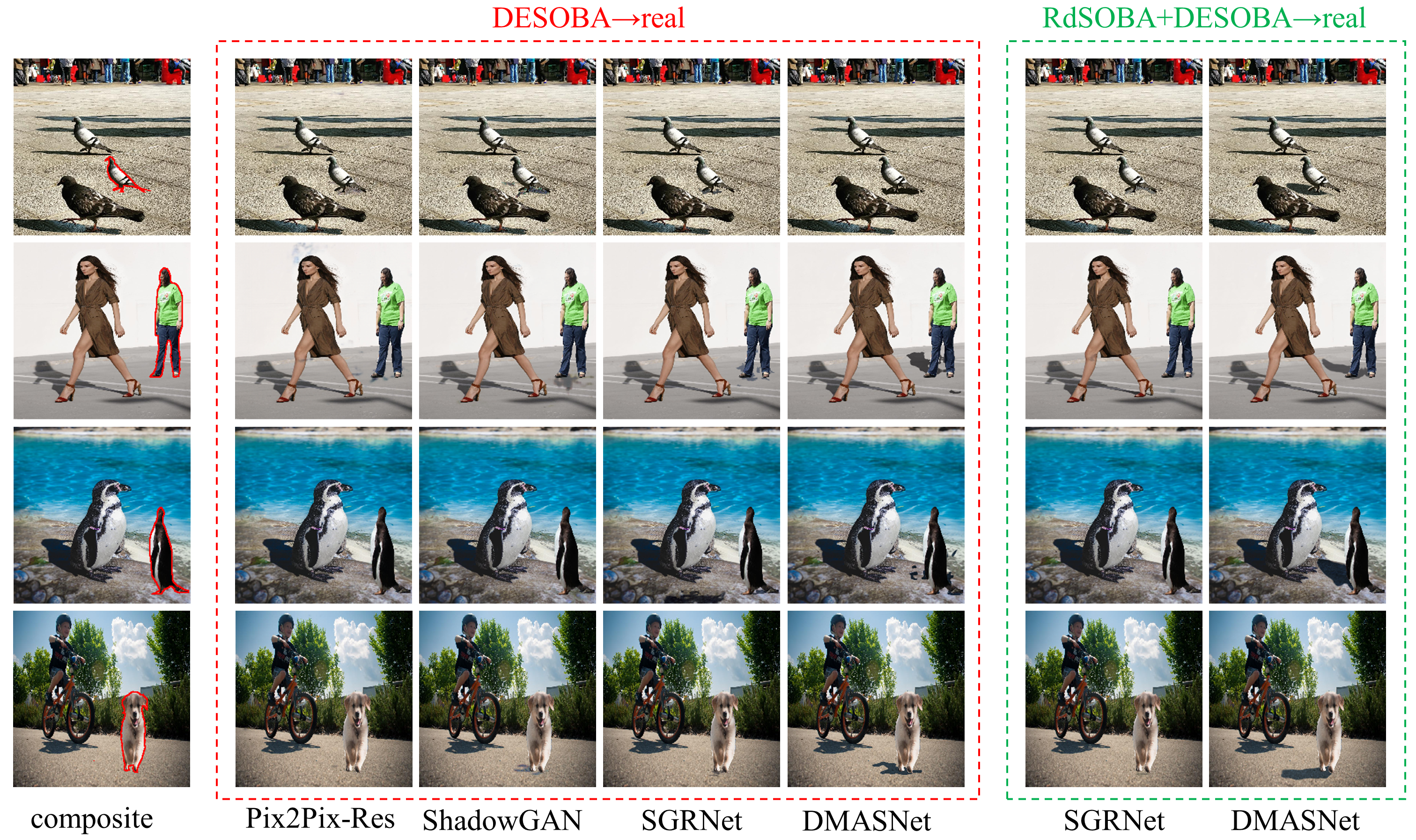
5.6 Evaluation on Real Composite Images
Our ultimate goal is generating realistic foreground shadow for real composite images, so we compare different methods on the 100 real composite images provided by (Hong, Niu, and Zhang 2022). We compare our DMASNet with SGRNet as well as relatively strong baselines Pix2Pix-Res and ShadowGAN (see Table 1). For DMASNet and SGRNet, we provide two versions depending on whether using RdSOBA dataset or not. As there are no ground-truth images, we report the metrics d_hole, d_frag and conduct user study. We only report d_hole, d_frag for DMASNet and SGRNet, because the other two methods do not predict mask.
In our user study, we invite 20 people to observe a pair of generated images by two methods at a time and ask them to choose the one with more realistic foreground shadow. Based on pairwise scores, we use Bradley-Terry(B-T) model (Bradley and Terry 1952) to calculate the global ranking score for each method. We list the results in Table 3 and show the generated images by different methods in Figure 5. We can see that our DMASNet can greatly benefit from RdSOBA and consistently produce more realistic results, while SGRNet fails to produce shadow in many cases.
6 Conclusion
In this work, we have contributed a large-scale rendered shadow generation dataset RdSOBA. We have also proposed a novel two-stage shadow generation network DMASNet, which decomposes mask prediction and performs attentive shadow filling. Extensive experiments have proved that our RdSOBA dataset is helpful. Our DMASNet has shown remarkable cross-domain transferability and achieved the best visual effects for real composite images.
Acknowledgements
The work was supported by the National Natural Science Foundation of China (Grant No. 62076162), the Shanghai Municipal Science and Technology Major/Key Project, China (Grant No. 2021SHZDZX0102, Grant No. 20511100300).
References
- Azadi et al. (2020) Azadi, S.; Pathak, D.; Ebrahimi, S.; and Darrell, T. 2020. Compositional gan: Learning image-conditional binary composition. International Journal of Computer Vision, 128(10): 2570–2585.
- Bradley and Terry (1952) Bradley, R. A.; and Terry, M. E. 1952. Rank analysis of incomplete block designs: I. The method of paired comparisons. Biometrika, 39(3/4): 324–345.
- Chen and Kae (2019) Chen, B.-C.; and Kae, A. 2019. Toward realistic image compositing with adversarial learning. In Proceedings of the IEEE/CVF Conference on Computer Vision and Pattern Recognition, 8415–8424.
- Chen et al. (2020) Chen, Z.; Zhu, L.; Wan, L.; Wang, S.; Feng, W.; and Heng, P.-A. 2020. A multi-task mean teacher for semi-supervised shadow detection. In Proceedings of the IEEE/CVF Conference on computer vision and pattern recognition, 5611–5620.
- Cong et al. (2022) Cong, W.; Tao, X.; Niu, L.; Liang, J.; Gao, X.; Sun, Q.; and Zhang, L. 2022. High-Resolution Image Harmonization via Collaborative Dual Transformations. In Proceedings of the IEEE/CVF Conference on Computer Vision and Pattern Recognition, 18470–18479.
- Ding et al. (2019) Ding, B.; Long, C.; Zhang, L.; and Xiao, C. 2019. Argan: Attentive recurrent generative adversarial network for shadow detection and removal. In Proceedings of the IEEE/CVF international conference on computer vision, 10213–10222.
- Guo et al. (2023) Guo, L.; Wang, C.; Yang, W.; Huang, S.; Wang, Y.; Pfister, H.; and Wen, B. 2023. Shadowdiffusion: When degradation prior meets diffusion model for shadow removal. In Proceedings of the IEEE/CVF Conference on Computer Vision and Pattern Recognition, 14049–14058.
- Guo et al. (2021) Guo, Z.; Guo, D.; Zheng, H.; Gu, Z.; Zheng, B.; and Dong, J. 2021. Image harmonization with transformer. In Proceedings of the IEEE/CVF International Conference on Computer Vision, 14870–14879.
- He et al. (2017) He, K.; Gkioxari, G.; Dollár, P.; and Girshick, R. 2017. Mask r-cnn. In Proceedings of the IEEE international conference on computer vision, 2961–2969.
- Hong, Niu, and Zhang (2022) Hong, Y.; Niu, L.; and Zhang, J. 2022. Shadow generation for composite image in real-world scenes. In Proceedings of the AAAI Conference on Artificial Intelligence, volume 36, 914–922.
- Hu et al. (2019) Hu, X.; Jiang, Y.; Fu, C.-W.; and Heng, P.-A. 2019. Mask-shadowgan: Learning to remove shadows from unpaired data. In Proceedings of the IEEE/CVF International Conference on Computer Vision, 2472–2481.
- Isola et al. (2017) Isola, P.; Zhu, J.-Y.; Zhou, T.; and Efros, A. A. 2017. Image-to-image translation with conditional adversarial networks. In Proceedings of the IEEE conference on computer vision and pattern recognition, 1125–1134.
- Karsch et al. (2014) Karsch, K.; Sunkavalli, K.; Hadap, S.; Carr, N.; Jin, H.; Fonte, R.; Sittig, M.; and Forsyth, D. 2014. Automatic scene inference for 3d object compositing. ACM Transactions on Graphics (TOG), 33(3): 1–15.
- Kee, O’brien, and Farid (2014) Kee, E.; O’brien, J. F.; and Farid, H. 2014. Exposing Photo Manipulation from Shading and Shadows. ACM Trans. Graph., 33(5): 165–1.
- Le and Samaras (2020) Le, H.; and Samaras, D. 2020. From shadow segmentation to shadow removal. In Computer Vision–ECCV 2020: 16th European Conference, Glasgow, UK, August 23–28, 2020, Proceedings, Part XI 16, 264–281. Springer.
- Lee et al. (2018) Lee, D.; Liu, S.; Gu, J.; Liu, M.-Y.; Yang, M.-H.; and Kautz, J. 2018. Context-aware synthesis and placement of object instances. Advances in neural information processing systems, 31.
- Liao et al. (2019) Liao, B.; Zhu, Y.; Liang, C.; Luo, F.; and Xiao, C. 2019. Illumination animating and editing in a single picture using scene structure estimation. Computers & Graphics, 82: 53–64.
- Lin et al. (2018) Lin, C.-H.; Yumer, E.; Wang, O.; Shechtman, E.; and Lucey, S. 2018. St-gan: Spatial transformer generative adversarial networks for image compositing. In Proceedings of the IEEE Conference on Computer Vision and Pattern Recognition, 9455–9464.
- Ling et al. (2021) Ling, J.; Xue, H.; Song, L.; Xie, R.; and Gu, X. 2021. Region-aware adaptive instance normalization for image harmonization. In Proceedings of the IEEE/CVF Conference on Computer Vision and Pattern Recognition, 9361–9370.
- Liu et al. (2020) Liu, D.; Long, C.; Zhang, H.; Yu, H.; Dong, X.; and Xiao, C. 2020. Arshadowgan: Shadow generative adversarial network for augmented reality in single light scenes. In Proceedings of the IEEE/CVF Conference on Computer Vision and Pattern Recognition, 8139–8148.
- Liu et al. (2021) Liu, L.; Zhang, B.; Li, J.; Niu, L.; Liu, Q.; and Zhang, L. 2021. OPA: Object Placement Assessment Dataset. arXiv preprint arXiv:2107.01889.
- Niu et al. (2021) Niu, L.; Cong, W.; Liu, L.; Hong, Y.; Zhang, B.; Liang, J.; and Zhang, L. 2021. Making images real again: A comprehensive survey on deep image composition. arXiv preprint arXiv:2106.14490.
- Sheng, Zhang, and Benes (2021) Sheng, Y.; Zhang, J.; and Benes, B. 2021. SSN: Soft shadow network for image compositing. In Proceedings of the IEEE/CVF Conference on Computer Vision and Pattern Recognition, 4380–4390.
- van Steenkiste et al. (2020) van Steenkiste, S.; Kurach, K.; Schmidhuber, J.; and Gelly, S. 2020. Investigating object compositionality in generative adversarial networks. Neural Networks, 130: 309–325.
- Wang et al. (2021) Wang, T.; Hu, X.; Fu, C.-W.; and Heng, P.-A. 2021. Single-stage instance shadow detection with bidirectional relation learning. In Proceedings of the IEEE/CVF Conference on Computer Vision and Pattern Recognition, 1–11.
- Weng et al. (2020) Weng, S.; Li, W.; Li, D.; Jin, H.; and Shi, B. 2020. Misc: Multi-condition injection and spatially-adaptive compositing for conditional person image synthesis. In Proceedings of the IEEE/CVF Conference on Computer Vision and Pattern Recognition, 7741–7749.
- Wu et al. (2019) Wu, H.; Zheng, S.; Zhang, J.; and Huang, K. 2019. Gp-gan: Towards realistic high-resolution image blending. In Proceedings of the 27th ACM international conference on multimedia, 2487–2495.
- Zhan et al. (2020) Zhan, F.; Lu, S.; Zhang, C.; Ma, F.; and Xie, X. 2020. Adversarial image composition with auxiliary illumination. In Proceedings of the Asian Conference on Computer Vision.
- Zhang et al. (2021) Zhang, H.; Zhang, J.; Perazzi, F.; Lin, Z.; and Patel, V. M. 2021. Deep image compositing. In Proceedings of the IEEE/CVF Winter Conference on Applications of Computer Vision, 365–374.
- Zhang et al. (2019) Zhang, J.; Sunkavalli, K.; Hold-Geoffroy, Y.; Hadap, S.; Eisenman, J.; and Lalonde, J.-F. 2019. All-weather deep outdoor lighting estimation. In Proceedings of the IEEE/CVF Conference on Computer Vision and Pattern Recognition, 10158–10166.
- Zhang et al. (2020a) Zhang, L.; Long, C.; Zhang, X.; and Xiao, C. 2020a. Ris-gan: Explore residual and illumination with generative adversarial networks for shadow removal. In Proceedings of the AAAI Conference on Artificial Intelligence, volume 34, 12829–12836.
- Zhang et al. (2020b) Zhang, L.; Wen, T.; Min, J.; Wang, J.; Han, D.; and Shi, J. 2020b. Learning object placement by inpainting for compositional data augmentation. In European Conference on Computer Vision, 566–581. Springer.
- Zhang, Wen, and Shi (2020) Zhang, L.; Wen, T.; and Shi, J. 2020. Deep image blending. In Proceedings of the IEEE/CVF Winter Conference on Applications of Computer Vision, 231–240.
- Zhang, Liang, and Wang (2019) Zhang, S.; Liang, R.; and Wang, M. 2019. Shadowgan: Shadow synthesis for virtual objects with conditional adversarial networks. Computational Visual Media, 5(1): 105–115.
- Zhang et al. (2020c) Zhang, S.-H.; Zhou, Z.-P.; Liu, B.; Dong, X.; and Hall, P. 2020c. What and where: A context-based recommendation system for object insertion. Computational Visual Media, 6(1): 79–93.
- Zheng et al. (2020) Zheng, Z.; Wang, P.; Liu, W.; Li, J.; Ye, R.; and Ren, D. 2020. Distance-IoU loss: Faster and better learning for bounding box regression. In Proceedings of the AAAI conference on artificial intelligence, volume 34, 12993–13000.
- Zhu et al. (2022) Zhu, Y.; Huang, J.; Fu, X.; Zhao, F.; Sun, Q.; and Zha, Z.-J. 2022. Bijective mapping network for shadow removal. In Proceedings of the IEEE/CVF Conference on Computer Vision and Pattern Recognition, 5627–5636.