Shape-conditioned 3D Molecule Generation via Equivariant Diffusion Models

Ziqi Chen¹, Bo Peng¹, Srinivasan Parthasarathy^1,2, Xia Ning^1,2,3 Contact author

Abstract

Ligand-based drug design aims to identify novel drug candidates of similar shapes with known active molecules. In this paper, we formulated an in silico shape-conditioned molecule generation problem to generate 3D molecule structures conditioned on the shape of a given molecule. To address this problem, we developed a translation- and rotation-equivariant shape-guided generative model $\mathop{\mathsf{ShapeMol}}\limits$ . $\mathop{\mathsf{ShapeMol}}\limits$ consists of an equivariant shape encoder that maps molecular surface shapes into latent embeddings, and an equivariant diffusion model that generates 3D molecules based on these embeddings. Experimental results show that $\mathop{\mathsf{ShapeMol}}\limits$ can generate novel, diverse, drug-like molecules that retain 3D molecular shapes similar to the given shape condition. These results demonstrate the potential of $\mathop{\mathsf{ShapeMol}}\limits$ in designing drug candidates of desired 3D shapes binding to protein target pockets.

Introduction

Generating novel drug candidates is a critical step in drug discovery to identify possible therapeutic solutions. Conventionally, this process is characterized based on knowledge and experience from medicinal chemists, and is resource- and time-consuming. Recently, computational approaches to molecule generation have been developed to accelerate the conventional paradigm. Existing molecular generative models largely focus on generating either molecule SMILES strings or molecular graphs (Gómez-Bombarelli et al. 2018; Jin, Barzilay, and Jaakkola 2018; Chen et al. 2021), with a recent shift towards 3D molecular structures. Several models (Luo et al. 2021; Peng et al. 2022; Guan et al. 2023) have been designed to generate 3D molecules conditioned on the protein targets, aiming to facilitate structured-based drug design (SBDD) (Batool, Ahmad, and Choi 2019), given that molecules exist in 3D space and the efficacy of drug molecules depends on their 3D structures fitting into protein pockets. However, SBDD relies on the availability of high-quality 3D structures of protein binding pockets, which are lacking for many targets (Zheng et al. 2013).

Different from SBDD, ligand-based drug design (LBDD) (Acharya et al. 2011) utilizes ligands known to interact with a protein target, and does not require knowledge of protein structures. In LBDD, shape-based virtual screening tools such as ROCS (Hawkins, Skillman, and Nicholls 2006) have been widely used to identify molecules with similar shapes to known ligands by enumerating molecules in chemical libraries. However, virtual screen tools cannot probe the novel chemical space. Therefore, it is highly needed to develop generative methods to generate novel molecules with desired 3D shapes.

In this paper, we present a novel generative model for 3D molecule generation conditioned on given 3D shapes. Our method, denoted to as $\mathop{\mathsf{ShapeMol}}\limits$ , employs an equivariant shape embedding module to map 3D molecule surface shapes into shape latent embeddings. It then uses a conditional diffusion generative model to generate molecules conditioned on the shape latent embeddings, by iteratively denoising atom positions and atom features (e.g., atom type and aromaticity). During molecule generation, $\mathop{\mathsf{ShapeMol}}\limits$ can utilize additional shape guidance by pushing the predicted atoms far from the condition shapes to those shapes. $\mathop{\mathsf{ShapeMol}}\limits$ with shape guidance is denoted as $\mathop{\mathsf{ShapeMol}\text{+}\mathsf{g}}\limits$ . The major contributions of this paper are as follows:

•

To the best of our knowledge, $\mathop{\mathsf{ShapeMol}}\limits$ is the first diffusion-based method for 3D molecule generation conditioned on 3D molecule shapes.
•

$\mathop{\mathsf{ShapeMol}}\limits$ leverages a new equivariant shape embedding module to learn 3D surface shape embeddings from cloud points sampled over molecule surfaces.
•

$\mathop{\mathsf{ShapeMol}}\limits$ uses a novel conditional diffusion model to generate 3D molecule structures. The diffusion model is equivariant to the translation and rotation of molecule shapes. A new weighting scheme over diffusion steps is developed to ensure accurate molecule shape prediction.
•

$\mathop{\mathsf{ShapeMol}}\limits$ utilizes new shape guidance to direct the generated molecules to better fit the shape condition.
•

$\mathop{\mathsf{ShapeMol}\text{+}\mathsf{g}}\limits$ achieves the highest average 3D shape similarity between the generated molecules and condition molecules, compared to the state-of-the-art baseline.

For reproducibility purposes, detailed parameters in all the experiments, code and data are reported in Supplementary Section LABEL:supp:experiments:parameters.

Related Work

Molecule Generation

A variety of deep generative models have been developed to generate molecules using various molecule representations, incliuding generating SMILES string representations (Gómez-Bombarelli et al. 2018), or 2D molecular graph representations (Jin, Barzilay, and Jaakkola 2018; Chen et al. 2021). Recent efforts have been dedicated to the generation of 3D molecules. These 3D molecule generative models can be divided into two categories: autoregressive models and non-autoregressive models. Autoregressive models generate 3D molecules by sequentially adding atoms into the 3D space (Luo et al. 2021; Peng et al. 2022). While these models ensure the validity and connectivity of generated molecules, any errors made in sequential predictions could accumulate in subsequent predictions. Non-autoregressive models generate 3D molecules using flow-based methods (Garcia Satorras et al. 2021) or diffusion methods (Guan et al. 2023). In these models, atoms are generated or adjusted all together. For example, Hoogeboom et al. (2022) developed an equivariant diffusion model, in which an equivariant network is employed to jointly predict both the positions and features of all atoms.

Shape-Conditioned Molecule Generation

Following the idea of ligand-based drug design (LBDD) (Acharya et al. 2011), previous work has been focused on generating molecules with similar 3D shapes to those of efficacy, based on the observation that structurally similar molecules tend to have similar properties. Papadopoulos et al. (2021) developed a reinforcement learning method to generate SMILES strings of molecules that are similar to known antagonists of DRD2 receptors in 3D shapes and pharmacophores. Imrie et al. (2021) generated 2D molecular graphs conditioned on 3D pharmacophores using a graph-based autoencoder. However, there is limited work that generates 3D molecule structures conditioned on 3D shapes. Adams and Coley (2023) developed a shape-conditioned generative framework $\mathop{\mathsf{SQUID}}\limits$ for 3D molecule generation. $\mathop{\mathsf{SQUID}}\limits$ learns a variational autoencoder to generate fragments conditioned on given 3D shapes, and decodes molecules by sequentially attaching fragments with fixed bond lengths and angles. While LBDD plays a vital role in drug discovery, the problem of generating 3D molecule structures conditioned on 3D shapes is still under-addressed.

Definitions and Notations

Problem Definition

Following Adams and Coley (2023), we focus on the 3D molecule generation conditioned on the shape of a given molecule (e.g., a ligand). Specifically, we aim to generate a new molecule $\mathop{\mathtt{M}_{y}}\limits$ , conditioned on the 3D shape of a given molecule $\mathop{\mathtt{M}_{x}}\limits$ , such that 1) $\mathop{\mathtt{M}_{y}}\limits$ is similar to $\mathop{\mathtt{M}_{x}}\limits$ in their 3D shapes, measured by $\mbox{$\mathop{\mathsf{Sim}_{\mathtt{s}}}\limits$}(\mbox{$\mathop{\mathtt{s}}\limits$}_{x},\mbox{$\mathop{\mathtt{s}}\limits$}_{y})$ , where $\mathop{\mathtt{s}}\limits$ is the 3D shape of $\mathop{\mathtt{M}}\limits$ ; and 2) $\mathop{\mathtt{M}_{y}}\limits$ is dissimilar to $\mathop{\mathtt{M}_{x}}\limits$ in their 2D molecular graph structures, measured by $\mbox{$\mathop{\mathsf{Sim}_{\mathtt{g}}}\limits$}(\mbox{$\mathop{\mathtt{M}_{x}}\limits$},\mbox{$\mathop{\mathtt{M}_{y}}\limits$})$ . This conditional 3D shape generation problem is motivated by the fact that in ligand-based drug design, it is desired to find chemically diverse and novel molecules that share similar shapes and similar activities with known active ligands (Ripphausen, Nisius, and Bajorath 2011). Such chemically diverse and novel molecules could expand the search space for drug candidates and potentially enhance the development of effective drugs.

Representations and Notations

We represent a molecule $\mathop{\mathtt{M}}\limits$ as a set of atoms $\mbox{$\mathop{\mathtt{M}}\limits$}=\{a_{1},a_{2},\cdots,a_{{|\mbox{$\mathop{\mathtt{M}}\limits$}|}}|a_{i}=(\mbox{$\mathop{\mathbf{x}}\limits$}_{i},\mbox{$\mathop{\mathbf{v}}$}_{i})\}$ , where $|\mbox{$\mathop{\mathtt{M}}\limits$}|$ is the number of atoms in $\mathop{\mathtt{M}}\limits$ ; $a_{i}$ is the $i$ -th atom in $\mathop{\mathtt{M}}\limits$ ; $\mbox{$\mathop{\mathbf{x}}\limits$}_{i}\in\mathbb{R}^{3}$ represents the 3D coordinates of $a_{i}$ ; and $\mbox{$\mathop{\mathbf{v}}$}_{i}\in\mathbb{R}^{K}$ is $a_{i}$ ’s one-hot atom feature vector indicating the atom type and its aromaticity. Following Guan et al. (2023), bonds between atoms can be uniquely determined by the atom types and the atomic distances among atoms. We represent the 3D surface shape $\mathop{\mathtt{s}}\limits$ of a molecule $\mathop{\mathtt{M}}\limits$ as a point cloud constructed by sampling points over the molecular surface. Details about the construction of point clouds from the surface of molecules are available in Supplementary Section LABEL:supp:point_clouds. We denote the point cloud as $\mbox{$\mathop{\mathcal{P}}\limits$}=\{z_{1},z_{2},\cdots\,z_{{|\mbox{$\mathop{\mathcal{P}}\limits$}|}}|z_{j}=(\mbox{$\mathop{\mathbf{z}}\limits$}_{j})\}$ , where $|\mbox{$\mathop{\mathcal{P}}\limits$}|$ is the number of points in $\mathop{\mathcal{P}}\limits$ ; $z_{j}$ is the $j$ -th point; and $\mbox{$\mathop{\mathbf{z}}\limits$}_{j}\in\mathbb{R}^{3}$ represents the 3D coordinates of $z_{j}$ . We denote the latent embedding of $\mathop{\mathcal{P}}\limits$ as $\mbox{$\mathop{\mathbf{H}^{\mathtt{s}}}\limits$}\in\mathbb{R}^{d_{p}\times 3}$ , where $d_{p}$ is the dimension of the latent embedding.

Method

$\mathop{\mathsf{ShapeMol}}\limits$ consists of an equivariant shape embedding module $\mathop{\mathsf{SE}}\limits$ that maps 3D molecular surface shapes to latent embeddings, and an equivariant diffusion model $\mathop{\mathsf{DIFF}}\limits$ that generates 3D molecules conditioned on these embeddings. Figure 1 presents the overall architecture of $\mathop{\mathsf{ShapeMol}}\limits$ .

Refer to caption — Figure 1: Model Architecture of $\mathop{\mathsf{ShapeMol}}\limits$

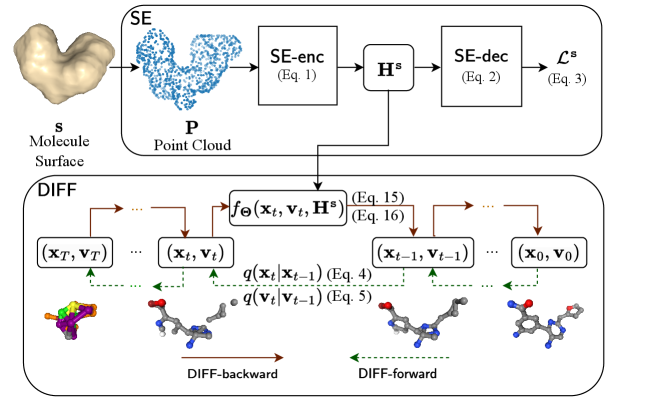
Equivariant Shape Embedding ( $\mathop{\mathsf{SE}}\limits$ )

$\mathop{\mathsf{ShapeMol}}\limits$ pre-trains a shape embedding module $\mathop{\mathsf{SE}}\limits$ to generate surface shape embeddings $\mathop{\mathbf{H}^{\mathtt{s}}}\limits$ . $\mathop{\mathsf{SE}}\limits$ uses an encoder $\mathop{\mathsf{SE}\text{-}\mathsf{enc}}\limits$ to map $\mathop{\mathcal{P}}\limits$ to the equivariant latent embedding $\mathop{\mathbf{H}^{\mathtt{s}}}\limits$ . $\mathop{\mathsf{SE}}\limits$ employs a decoder $\mathop{\mathsf{SE}\text{-}\mathsf{dec}}\limits$ to optimize $\mathop{\mathbf{H}^{\mathtt{s}}}\limits$ by recovering the signed distances (Park et al. 2019) of sampled query points in 3D space to the molecule surface based on $\mathop{\mathbf{H}^{\mathtt{s}}}\limits$ . $\mathop{\mathsf{ShapeMol}}\limits$ uses $\mbox{$\mathop{\mathbf{H}}\limits$}^{\mathtt{s}}$ to guide the diffusion process later.

Shape Encoder ( $\mathop{\mathsf{SE}\text{-}\mathsf{enc}}\limits$ )

$\mathop{\mathsf{SE}\text{-}\mathsf{enc}}\limits$ generates equivariant shape embeddings $\mbox{$\mathop{\mathbf{H}}\limits$}^{\mathtt{s}}$ from the 3D surface shape $\mathop{\mathcal{P}}\limits$ of molecules, such that $\mbox{$\mathop{\mathbf{H}}\limits$}^{\mathtt{s}}$ is equivariant to both translation and rotation of $\mathop{\mathcal{P}}\limits$ . That is, any translation and rotation applied to $\mathop{\mathcal{P}}\limits$ is reflected in $\mbox{$\mathop{\mathbf{H}}\limits$}^{\mathtt{s}}$ accordingly. To ensure translation equivariance, $\mathop{\mathsf{SE}\text{-}\mathsf{enc}}\limits$ shifts the center of each $\mathop{\mathcal{P}}\limits$ to zero to eliminate all translations. To ensure rotation equivariance, $\mathop{\mathsf{SE}\text{-}\mathsf{enc}}\limits$ leverages Vector Neurons (VNs) (Deng et al. 2021) and Dynamic Graph Convolutional Neural Networks (DGCNNs) (Wang et al. 2019) as follows:

\{\mbox{$\mathop{\mathbf{H}}\limits$}^{\mathtt{p}}_{1},\mbox{$\mathop{\mathbf{H}}\limits$}^{\mathtt{p}}_{2},\cdots,\mbox{$\mathop{\mathbf{H}}\limits$}^{\mathtt{p}}_{|{\mbox{$\mathop{\mathcal{P}}\limits$}}|}\}=\text{VN-DGCNN}(\{\mbox{$\mathop{\mathbf{z}}\limits$}_{1},\mbox{$\mathop{\mathbf{z}}\limits$}_{2},\cdots,\mbox{$\mathop{\mathbf{z}}\limits$}_{|{\mbox{$\mathop{\mathcal{P}}\limits$}}|}\}),\vspace{-5pt}

\mbox{$\mathop{\mathbf{H}}\limits$}^{\mathtt{s}}=\sum\nolimits_{j}\mbox{$\mathop{\mathbf{H}}\limits$}^{\mathtt{p}}_{j}/{|\mbox{$\mathop{\mathcal{P}}\limits$}|},

where $\text{VN-DGCNN}(\cdot)$ is a VN-based DGCNN network to generate equivariant embedding $\mbox{$\mathop{\mathbf{H}}\limits$}^{\mathtt{p}}_{j}\in\mathbb{R}^{d_{p}\times 3}$ for each point $z_{j}$ in $\mathop{\mathcal{P}}\limits$ ; and $\mbox{$\mathop{\mathbf{H}}\limits$}^{\mathtt{s}}\in\mathbb{R}^{d_{p}\times 3}$ is the embedding of $\mathop{\mathcal{P}}\limits$ generated via a mean-pooling over the embeddings of all the points. Note that $\text{VN-DGCNN}(\cdot)$ generates a matrix as the embedding of each point (i.e., $\mbox{$\mathop{\mathbf{H}}\limits$}^{\mathtt{p}}_{j}$ ) to guarantee the equivariance.

Shape Decoder ( $\mathop{\mathsf{SE}\text{-}\mathsf{dec}}\limits$ )

To optimize $\mbox{$\mathop{\mathbf{H}}\limits$}^{\mathtt{s}}$ , $\mathop{\mathsf{SE}}\limits$ learns a decoder $\mathop{\mathsf{SE}\text{-}\mathsf{dec}}\limits$ to predict the signed distance of a query point $z_{q}$ sampled from 3D space using Multilayer Perceptrons (MLPs) as follows:

\tilde{o}_{q}=\text{MLP}(\text{concat}(\langle\mathbf{z}_{q},\mbox{$\mathop{\mathbf{H}}\limits$}^{\mathtt{s}}\rangle,\|\mathbf{z}_{q}\|^{2},\text{VN-In}(\mbox{$\mathop{\mathbf{H}}\limits$}^{\mathtt{s}}))),

(1)

where $\tilde{o}_{q}$ is the predicted signed distance of $z_{q}$ , with positive and negative values indicating $z_{q}$ is inside or outside the surface shape, respectively; $\langle\cdot,\cdot\rangle$ is the dot-product operator; $\|\mathbf{z}_{q}\|^{2}$ is the Euclidean norm of the coordinates of $z_{q}$ ; $\text{VN-In}(\cdot)$ is an invariant VN network (Deng et al. 2021) that converts the equivariant shape embedding $\mbox{$\mathop{\mathbf{H}^{\mathtt{s}}}\limits$}\in\mathbb{R}^{d_{p}\times 3}$ into an invariant shape embedding. Thus, $\mathop{\mathsf{SE}\text{-}\mathsf{dec}}\limits$ predicts the signed distance between the query point and 3D surface by jointly considering the position of the query point ( $\|\mathbf{z}_{q}\|^{2}$ ), the molecular surface shape ( $\text{VN-In}(\cdot)$ ) and the interaction between the point and surface $\langle\cdot,\cdot\rangle$ . The predicted signed distance $\tilde{o}_{q}$ is used to calculate the loss for the optimization of $\mathop{\mathbf{H}^{\mathtt{s}}}\limits$ (discussed below). As shown in the literature (Deng et al. 2021), $\tilde{o}_{q}$ remains invariant to the rotation of the 3D molecule surface shapes (i.e., $\mathop{\mathcal{P}}\limits$ ). We present the sampling process of $z_{q}$ in the Supplementary Section LABEL:supp:training:shapeemb.

$\mathop{\mathsf{SE}}\limits$ Pre-training

$\mathop{\mathsf{ShapeMol}}\limits$ pre-trains $\mathop{\mathsf{SE}}\limits$ by minimizing the squared-errors loss between the predicted and the ground-truth signed distances of query points as follows:

\mathcal{L}^{\mathtt{s}}=\sum\nolimits_{z_{q}\in\mathcal{Z}}\|o_{q}-\tilde{o}_{q}\|^{2},

(2)

where $\mathcal{Z}$ is the set of sampled query points and $o_{q}$ is the ground-truth signed distance of query point $z_{q}$ . By pretraining $\mathop{\mathsf{SE}}\limits$ , $\mathop{\mathsf{ShapeMol}}\limits$ learns $\mathop{\mathbf{H}^{\mathtt{s}}}\limits$ that will be used as the condition in the following 3D molecule generation.

Shape-Conditioned Molecule Generation

In $\mathop{\mathsf{ShapeMol}}\limits$ , a shape-conditioned molecule diffusion model, referred to as $\mathop{\mathsf{DIFF}}\limits$ , is used to generate a 3D molecule structure (i.e., atom coordinates and features) conditioned on a given 3D surface shape that is represented by the shape latent embedding $\mathop{\mathbf{H}^{\mathtt{s}}}\limits$ (Eq. Shape Encoder ( $\mathop{\mathsf{SE}\text{-}\mathsf{enc}}\limits$ )). Following the denoising diffusion probabilistic models (Ho, Jain, and Abbeel 2020), $\mathop{\mathsf{DIFF}}\limits$ includes a forward diffusion process based on a Markov chain, denoted as $\mathop{\mathsf{DIFF}\text{-}\mathsf{forward}}\limits$ , which gradually adds noises step by step to the atom positions and features $\{(\mbox{$\mathop{\mathbf{x}}\limits$}_{i},\mbox{$\mathop{\mathbf{v}}$}_{i})\}$ in the training molecules. The noisy atom positions and features at step $t$ are represented as $\{(\mbox{$\mathop{\mathbf{x}}\limits$}_{i,t},\mbox{$\mathop{\mathbf{v}}$}_{i,t})\}$ ( $t=1,\cdots,T$ ), and the molecules without any noise are represented as $\{(\mbox{$\mathop{\mathbf{x}}\limits$}_{i,0},\mbox{$\mathop{\mathbf{v}}$}_{i,0})\}$ . At the final step $T$ , $\{(\mbox{$\mathop{\mathbf{x}}\limits$}_{i,T},\mbox{$\mathop{\mathbf{v}}$}_{i,T})\}$ are completely unstructured and resemble a simple distribution like a Normal distribution $\mathcal{N}(\mathbf{0},\mathbf{I})$ or a uniform categorical distribution $\mathcal{C}(\mathbf{1}/K)$ , in which $\mathbf{I}$ and $\mathbf{1}$ denotes the identity matrix and identity vector, respectively.

During training, $\mathop{\mathsf{DIFF}}\limits$ is learned to reverse the forward diffusion process via another Markov chain, referred to as the backward generative process and denoted as $\mathop{\mathsf{DIFF}\text{-}\mathsf{backward}}\limits$ , to remove the noises in the noisy molecules. During inference, $\mathop{\mathsf{DIFF}}\limits$ first samples noisy atom positions and features at step $T$ from simple distributions and then generates a 3D molecule structure by removing the noises in the noisy molecules step by step until $t$ reaches 1.

Forward Diffusion Process ( $\mathop{\mathsf{DIFF}\text{-}\mathsf{forward}}\limits$ )

Following the previous work (Guan et al. 2023), at step $t\in[1,T]$ , a small Gaussian noise and a small categorical noise are added to the continuous atom positions and discrete atom features $\{(\mbox{$\mathop{\mathbf{x}}\limits$}_{i,t-1},\mbox{$\mathop{\mathbf{v}}$}_{i,t-1})\}$ , respectively. When no ambiguity arises, we will eliminate subscript $i$ in the notations and use $(\mbox{$\mathop{\mathbf{x}}\limits$}_{t-1},\mbox{$\mathop{\mathbf{v}}$}_{t-1})$ for brevity. The noise levels of the Gaussian and categorical noises are determined by two predefined variance schedules $(\beta_{t}^{\mathtt{x}},\beta_{t}^{\mathtt{v}})\in(0,1)$ , where $\beta_{t}^{\mathtt{x}}$ and $\beta_{t}^{\mathtt{v}}$ are selected to be sufficiently small to ensure the smoothness of $\mathop{\mathsf{DIFF}\text{-}\mathsf{forward}}\limits$ . The details about variance schedules are available in Supplementary Section LABEL:supp:forward:variance. Formally, for atom positions, the probability of $\mbox{$\mathop{\mathbf{x}}\limits$}_{t}$ sampled given $\mbox{$\mathop{\mathbf{x}}\limits$}_{t-1}$ , denoted as $q(\mbox{$\mathop{\mathbf{x}}\limits$}_{t}|\mbox{$\mathop{\mathbf{x}}\limits$}_{t-1})$ , is defined as follows,

q(\mbox{$\mathop{\mathbf{x}}\limits$}_{t}|\mbox{$\mathop{\mathbf{x}}\limits$}_{t-1})=\mathcal{N}(\mbox{$\mathop{\mathbf{x}}\limits$}_{t}|\sqrt{1-\beta^{\mathtt{x}}_{t}}\mbox{$\mathop{\mathbf{x}}\limits$}_{t-1},\beta^{\mathtt{x}}_{t}\mathbf{I}),

(3)

where $\mathcal{N}(\cdot)$ is a Gaussian distribution of $\mbox{$\mathop{\mathbf{x}}\limits$}_{t}$ with mean $\sqrt{1-\beta_{t}^{\mathtt{x}}}\mbox{$\mathop{\mathbf{x}}\limits$}_{t-1}$ and covariance $\beta_{t}^{\mathtt{x}}\mathbf{I}$ . Following Hoogeboom et al. (2021), for atom features, the probability of $\mbox{$\mathop{\mathbf{v}}$}_{t}$ across $K$ classes given $\mbox{$\mathop{\mathbf{v}}$}_{t-1}$ is defined as follows,

q(\mbox{$\mathop{\mathbf{v}}$}_{t}|\mbox{$\mathop{\mathbf{v}}$}_{t-1})=\mathcal{C}(\mbox{$\mathop{\mathbf{v}}$}_{t}|(1-\beta^{\mathtt{v}}_{t})\mbox{$\mathop{\mathbf{v}}$}_{t-1}+\beta^{\mathtt{v}}_{t}\mathbf{1}/K),

(4)

where $\mathcal{C}$ is a categorical distribution of $\mbox{$\mathop{\mathbf{v}}$}_{t}$ derived by noising $\mbox{$\mathop{\mathbf{v}}$}_{t-1}$ with a uniform noise $\beta^{\mathtt{v}}_{t}\mathbf{1}/K$ across $K$ classes.

Since the above distributions form Markov chains, the probability of any $\mbox{$\mathop{\mathbf{x}}\limits$}_{t}$ or $\mbox{$\mathop{\mathbf{v}}$}_{t}$ can be derived from $\mbox{$\mathop{\mathbf{x}}\limits$}_{0}$ or $\mbox{$\mathop{\mathbf{v}}$}_{0}$ :

$\displaystyle q(\mbox{$\mathop{\mathbf{x}}\limits$}_{t}\|\mbox{$\mathop{\mathbf{x}}\limits$}_{0})$	$\displaystyle=\mathcal{N}(\mbox{$\mathop{\mathbf{x}}\limits$}_{t}\|\sqrt{\mbox{$\mathop{\bar{\alpha}}\limits$}^{\mathtt{x}}_{t}}\mbox{$\mathop{\mathbf{x}}\limits$}_{0},(1-\mbox{$\mathop{\bar{\alpha}}\limits$}^{\mathtt{x}}_{t})\mathbf{I}),$	(5)
$\displaystyle q(\mbox{$\mathop{\mathbf{v}}$}_{t}\|\mbox{$\mathop{\mathbf{v}}$}_{0})$	$\displaystyle=\mathcal{C}(\mbox{$\mathop{\mathbf{v}}$}_{t}\|\mbox{$\mathop{\bar{\alpha}}\limits$}^{\mathtt{v}}_{t}\mbox{$\mathop{\mathbf{v}}$}_{0}+(1-\mbox{$\mathop{\bar{\alpha}}\limits$}^{\mathtt{v}}_{t})\mathbf{1}/K),$	(6)
$\displaystyle\text{where }\mbox{$\mathop{\bar{\alpha}}\limits$}^{\mathtt{u}}_{t}$	$\displaystyle=\prod\nolimits_{\tau=1}^{t}\alpha^{\mathtt{u}}_{\tau},\ \alpha^{\mathtt{u}}_{\tau}=1-\beta^{\mathtt{u}}_{\tau},\ {\mathtt{u}}={\mathtt{x}}\text{ or }{\mathtt{v}}.\;\;\;$	(7)

Note that $\bar{\alpha}^{\mathtt{u}}_{t}$ ( $\mathtt{u}={\mathtt{x}}\text{ or }{\mathtt{v}}$ ) is monotonically decreasing from 1 to 0 over $t=[1,T]$ . As $t\rightarrow 1$ , $\mbox{$\mathop{\bar{\alpha}}\limits$}^{\mathtt{x}}_{t}$ and $\mbox{$\mathop{\bar{\alpha}}\limits$}^{\mathtt{v}}_{t}$ are close to 1, leading to that $\mbox{$\mathop{\mathbf{x}}\limits$}_{t}$ or $\mbox{$\mathop{\mathbf{v}}$}_{t}$ approximates $\mbox{$\mathop{\mathbf{x}}\limits$}_{0}$ or $\mbox{$\mathop{\mathbf{v}}$}_{0}$ . Conversely, as $t\rightarrow T$ , $\mbox{$\mathop{\bar{\alpha}}\limits$}^{\mathtt{x}}_{t}$ and $\mbox{$\mathop{\bar{\alpha}}\limits$}^{\mathtt{v}}_{t}$ are close to 0, leading to that $q(\mbox{$\mathop{\mathbf{x}}\limits$}_{T}|\mbox{$\mathop{\mathbf{x}}\limits$}_{0})$ resembles $\mathcal{N}(\mathbf{0},\mathbf{I})$ and $q(\mbox{$\mathop{\mathbf{v}}$}_{T}|\mbox{$\mathop{\mathbf{v}}$}_{0})$ resembles $\mathcal{C}(\mathbf{1}/K)$ .

Using Bayes theorem, the ground-truth Normal posterior of atom positions $p(\mbox{$\mathop{\mathbf{x}}\limits$}_{t-1}|\mbox{$\mathop{\mathbf{x}}\limits$}_{t},\mbox{$\mathop{\mathbf{x}}\limits$}_{0})$ can be calculated in a closed-form (Ho, Jain, and Abbeel 2020) as below,

	$\displaystyle p(\mbox{$\mathop{\mathbf{x}}\limits$}_{t-1}\|\mbox{$\mathop{\mathbf{x}}\limits$}_{t},\mbox{$\mathop{\mathbf{x}}\limits$}_{0})=\mathcal{N}(\mbox{$\mathop{\mathbf{x}}\limits$}_{t-1}\|\mu(\mbox{$\mathop{\mathbf{x}}\limits$}_{t},\mbox{$\mathop{\mathbf{x}}\limits$}_{0}),\tilde{\beta}^{\mathtt{x}}_{t}\mathbf{I}),$		(8)
	$\displaystyle\!\!\!\!\!\!\!\!\!\!\!\mu(\mbox{$\mathop{\mathbf{x}}\limits$}_{t},\mbox{$\mathop{\mathbf{x}}\limits$}_{0})\!=\!\frac{\sqrt{\bar{\alpha}^{\mathtt{x}}_{t-1}}\beta^{\mathtt{x}}_{t}}{1-\bar{\alpha}^{\mathtt{x}}_{t}}\mbox{$\mathop{\mathbf{x}}\limits$}_{0}\!+\!\frac{\sqrt{\alpha^{\mathtt{x}}_{t}}(1-\bar{\alpha}^{\mathtt{x}}_{t-1})}{1-\bar{\alpha}^{\mathtt{x}}_{t}}\mbox{$\mathop{\mathbf{x}}\limits$}_{t},\tilde{\beta}^{\mathtt{x}}_{t}\!=\!\frac{1-\bar{\alpha}^{\mathtt{x}}_{t-1}}{1-\bar{\alpha}^{\mathtt{x}}_{t}}\beta^{\mathtt{x}}_{t}.\;\;\;$		(9)

Similarly, the ground-truth categorical posterior of atom features $p(\mbox{$\mathop{\mathbf{v}}$}_{t-1}|\mbox{$\mathop{\mathbf{v}}$}_{t},\mbox{$\mathop{\mathbf{v}}$}_{0})$ can be calculated (Hoogeboom et al. 2021) as below,

	$\displaystyle p(\mbox{$\mathop{\mathbf{v}}$}_{t-1}\|\mbox{$\mathop{\mathbf{v}}$}_{t},\mbox{$\mathop{\mathbf{v}}$}_{0})=\mathcal{C}(\mbox{$\mathop{\mathbf{v}}$}_{t-1}\|\mathbf{c}(\mbox{$\mathop{\mathbf{v}}$}_{t},\mbox{$\mathop{\mathbf{v}}$}_{0})),$		(10)
	$\displaystyle\mathbf{c}(\mbox{$\mathop{\mathbf{v}}$}_{t},\mbox{$\mathop{\mathbf{v}}$}_{0})=\tilde{\mathbf{c}}/{\sum_{k=1}^{K}\tilde{c}_{k}},$		(11)
	$\displaystyle\tilde{\mathbf{c}}=[\alpha^{\mathtt{v}}_{t}\mbox{$\mathop{\mathbf{v}}$}_{t}+\frac{1-\alpha^{\mathtt{v}}_{t}}{K}]\odot[\bar{\alpha}^{\mathtt{v}}_{t-1}\mbox{$\mathop{\mathbf{v}}$}_{0}+\frac{1-\bar{\alpha}^{\mathtt{v}}_{t-1}}{K}],$		(12)

where $\tilde{c}_{k}$ denotes the likelihood of $k$ -th class across $K$ classes in $\tilde{\mathbf{c}}$ ; $\odot$ denotes the element-wise product operation; $\tilde{\mathbf{c}}$ is calculated using $\mbox{$\mathop{\mathbf{v}}$}_{t}$ and $\mbox{$\mathop{\mathbf{v}}$}_{0}$ and normalized so as to represent probabilities. The proof of the above equations is available in Supplementary Section LABEL:supp:forward:proof.

Backward Generative Process ( $\mathop{\mathsf{DIFF}\text{-}\mathsf{backward}}\limits$ )

$\mathop{\mathsf{DIFF}}\limits$ learns to reverse $\mathop{\mathsf{DIFF}\text{-}\mathsf{forward}}\limits$ by denoising from $(\mbox{$\mathop{\mathbf{x}}\limits$}_{t},\mbox{$\mathop{\mathbf{v}}$}_{t})$ to $(\mbox{$\mathop{\mathbf{x}}\limits$}_{t-1},\mbox{$\mathop{\mathbf{v}}$}_{t-1})$ at $t\in[1,T]$ , conditioned on the shape latent embedding $\mathop{\mathbf{H}^{\mathtt{s}}}\limits$ . Specifically, the probabilities of $(\mbox{$\mathop{\mathbf{x}}\limits$}_{t-1},\mbox{$\mathop{\mathbf{v}}$}_{t-1})$ denoised from $(\mbox{$\mathop{\mathbf{x}}\limits$}_{t},\mbox{$\mathop{\mathbf{v}}$}_{t})$ are estimated by the approximates of the ground-truth posteriors $p(\mbox{$\mathop{\mathbf{x}}\limits$}_{t-1}|\mbox{$\mathop{\mathbf{x}}\limits$}_{t},\mbox{$\mathop{\mathbf{x}}\limits$}_{0})$ (Eq. 8) and $p(\mbox{$\mathop{\mathbf{v}}$}_{t-1}|\mbox{$\mathop{\mathbf{v}}$}_{t},\mbox{$\mathop{\mathbf{v}}$}_{0})$ (Eq. 10). Given that $(\mbox{$\mathop{\mathbf{x}}\limits$}_{0},\mbox{$\mathop{\mathbf{v}}$}_{0})$ is unknown in the generative process, a predictor $f_{\boldsymbol{\Theta}}(\mbox{$\mathop{\mathbf{x}}\limits$}_{t},\mbox{$\mathop{\mathbf{v}}$}_{t},\mbox{$\mathop{\mathbf{H}^{\mathtt{s}}}\limits$})$ is employed to predict at $t$ the atom position and feature $(\mbox{$\mathop{\mathbf{x}}\limits$}_{0},\mbox{$\mathop{\mathbf{v}}$}_{0})$ as below,

(\tilde{\mbox{$\mathop{\mathbf{x}}\limits$}}_{0,t},\tilde{\mbox{$\mathop{\mathbf{v}}$}}_{0,t})=f_{\boldsymbol{\Theta}}(\mbox{$\mathop{\mathbf{x}}\limits$}_{t},\mbox{$\mathop{\mathbf{v}}$}_{t},\mbox{$\mathop{\mathbf{H}}\limits$}^{\mathtt{s}}),

(13)

where $\tilde{\mbox{$\mathop{\mathbf{x}}\limits$}}_{0,t}$ and $\tilde{\mbox{$\mathop{\mathbf{v}}$}}_{0,t}$ are the predictions of $\mbox{$\mathop{\mathbf{x}}\limits$}_{0}$ and $\mbox{$\mathop{\mathbf{v}}$}_{0}$ at $t$ ; ${\boldsymbol{\Theta}}$ is the learnable parameter. Following Ho et al. (2020), with $\tilde{\mbox{$\mathop{\mathbf{x}}\limits$}}_{0,t}$ , the probability of $\mbox{$\mathop{\mathbf{x}}\limits$}_{t-1}$ denoised from $\mbox{$\mathop{\mathbf{x}}\limits$}_{t}$ , denoted as $p(\mbox{$\mathop{\mathbf{x}}\limits$}_{t-1}|\mbox{$\mathop{\mathbf{x}}\limits$}_{t})$ , can be estimated by the approximated posterior $p_{\boldsymbol{\Theta}}((\mbox{$\mathop{\mathbf{x}}\limits$}_{t-1}|\mbox{$\mathop{\mathbf{x}}\limits$}_{t},\tilde{\mbox{$\mathop{\mathbf{x}}\limits$}}_{0,t})$ as below,

	$\displaystyle p(\mbox{$\mathop{\mathbf{x}}\limits$}_{t-1}\|\mbox{$\mathop{\mathbf{x}}\limits$}_{t})$	$\displaystyle\approx p_{\boldsymbol{\Theta}}(\mbox{$\mathop{\mathbf{x}}\limits$}_{t-1}\|\mbox{$\mathop{\mathbf{x}}\limits$}_{t},\tilde{\mbox{$\mathop{\mathbf{x}}\limits$}}_{0,t})$		(14)
		$\displaystyle=\mathcal{N}(\mbox{$\mathop{\mathbf{x}}\limits$}_{t-1}\|\mu_{\boldsymbol{\Theta}}(\mbox{$\mathop{\mathbf{x}}\limits$}_{t},\tilde{\mbox{$\mathop{\mathbf{x}}\limits$}}_{0,t}),\tilde{\beta}^{\mathtt{x}}_{t}\mathbf{I}),$		(14)

where $\mu_{\boldsymbol{\Theta}}(\mbox{$\mathop{\mathbf{x}}\limits$}_{t},\tilde{\mbox{$\mathop{\mathbf{x}}\limits$}}_{0,t})$ is an estimate of $\mu(\mbox{$\mathop{\mathbf{x}}\limits$}_{t},\mbox{$\mathop{\mathbf{x}}\limits$}_{0})$ by replacing $\mbox{$\mathop{\mathbf{x}}\limits$}_{0}$ with its estimate $\tilde{\mbox{$\mathop{\mathbf{x}}\limits$}}_{0,t}$ in Eq. 8. Similarly, with $\tilde{\mbox{$\mathop{\mathbf{v}}$}}_{0,t}$ , the probability of $\mbox{$\mathop{\mathbf{v}}$}_{t-1}$ denoised from $\mbox{$\mathop{\mathbf{v}}$}_{t}$ , denoted as $p(\mbox{$\mathop{\mathbf{v}}$}_{t-1}|\mbox{$\mathop{\mathbf{v}}$}_{t})$ , can be estimated by the approximated posterior $p_{\boldsymbol{\Theta}}(\mbox{$\mathop{\mathbf{v}}$}_{t-1}|\mbox{$\mathop{\mathbf{v}}$}_{t},\tilde{\mbox{$\mathop{\mathbf{v}}$}}_{0,t})$ as below,

\displaystyle\!\!\!\!\!\!\!\!p(\mbox{$\mathop{\mathbf{v}}$}_{t-1}|\mbox{$\mathop{\mathbf{v}}$}_{t})\!\!\approx\!\!p_{\boldsymbol{\Theta}}(\mbox{$\mathop{\mathbf{v}}$}_{t-1}|\mbox{$\mathop{\mathbf{v}}$}_{t},\tilde{\mbox{$\mathop{\mathbf{v}}$}}_{0,t})\!\!=\!\!\mathcal{C}(\mbox{$\mathop{\mathbf{v}}$}_{t-1}|\mathbf{c}_{\boldsymbol{\Theta}}(\mbox{$\mathop{\mathbf{v}}$}_{t},\tilde{\mbox{$\mathop{\mathbf{v}}$}}_{0,t})),

(15)

where $\mathbf{c}_{\boldsymbol{\Theta}}(\mbox{$\mathop{\mathbf{v}}$}_{t},\tilde{\mbox{$\mathop{\mathbf{v}}$}}_{0,t})$ is an estimate of $\mathbf{c}(\mbox{$\mathop{\mathbf{v}}$}_{t},\mbox{$\mathop{\mathbf{v}}$}_{0})$ by replacing $\mbox{$\mathop{\mathbf{v}}$}_{0}$ with its estimate $\tilde{\mbox{$\mathop{\mathbf{v}}$}}_{0,t}$ in Eq. 10.

Equivariant Shape-Conditioned Molecule Predictor

In $\mathop{\mathsf{DIFF}\text{-}\mathsf{backward}}\limits$ , the predictor $f_{\boldsymbol{\Theta}}(\mbox{$\mathop{\mathbf{x}}\limits$}_{t},\mbox{$\mathop{\mathbf{v}}$}_{t},\mbox{$\mathop{\mathbf{H}^{\mathtt{s}}}\limits$})$ (Eq. 13) predicts the atom positions and features $(\tilde{\mbox{$\mathop{\mathbf{x}}\limits$}}_{0,t},\tilde{\mbox{$\mathop{\mathbf{v}}$}}_{0,t})$ given the noisy data $(\mbox{$\mathop{\mathbf{x}}\limits$}_{t},\mbox{$\mathop{\mathbf{v}}$}_{t})$ conditioned on $\mathop{\mathbf{H}^{\mathtt{s}}}\limits$ . For brevity, in this subsection, we eliminate the subscript $t$ in the notations when no ambiguity arises. $f_{\boldsymbol{\Theta}}(\cdot)$ leverages two multi-layer graph neural networks: (1) an equivariant graph neural network, denoted as $\mathop{\mathsf{EQ}\text{-}\mathsf{GNN}}\limits$ , that equivariantly predicts atom positions that change under transformations, and (2) an invariant graph neural network, denoted as $\mathop{\mathsf{INV}\text{-}\mathsf{GNN}}\limits$ , that invariantly predicts atom features that remain unchanged under transformations. Following the previous work (Guan et al. 2023; Hoogeboom et al. 2022), the translation equivariance of atom position prediction is achieved by shifting a fixed point (e.g., the center of point clouds $\mathop{\mathcal{P}}\limits$ ) to zero, and therefore only rotation equivariance needs to be considered.

Atom Coordinate Prediction

In $\mathop{\mathsf{EQ}\text{-}\mathsf{GNN}}\limits$ , the atom position $\mbox{$\mathop{\mathbf{x}}\limits$}_{i}^{l+1}\in\mathbb{R}^{3}$ of $a_{i}$ at the ( $l$ +1)-th layer is calculated in an equivariant way as below,

\Delta\mbox{$\mathop{\mathbf{x}}\limits$}_{i}^{l+1}\!=\sum_{\mathclap{j\in N(a_{i}),i\neq j}}(\mbox{$\mathop{\mathbf{x}}\limits$}_{i}^{l}-\mbox{$\mathop{\mathbf{x}}\limits$}_{j}^{l})\text{MHA}^{\mathtt{x}}(d_{ij}^{l},\mbox{$\mathop{\mathbf{h}}\limits$}_{i}^{l+1},\mbox{$\mathop{\mathbf{h}}\limits$}_{j}^{l+1},\text{VN-In}(\mbox{$\mathop{\mathbf{H}^{\mathtt{s}}}\limits$})),

\mbox{$\mathop{\mathbf{x}}\limits$}_{i}^{l+1}\!=\mbox{$\mathop{\mathbf{x}}\limits$}_{i}^{l}\!+\!\text{Mean}(\Delta{\mbox{$\mathop{\mathbf{x}}\limits$}_{i}^{l+1}})\!+\!\text{VN-Lin}(\mbox{$\mathop{\mathbf{x}}\limits$}_{i}^{l},\Delta\mbox{$\mathop{\mathbf{x}}\limits$}_{i}^{l+1},\mbox{$\mathop{\mathbf{H}^{\mathtt{s}}}\limits$}),

(16)

where $N(a_{i})$ is the set of $N$ -nearest neighbors of $a_{i}$ based on atomic distances; $\Delta\mbox{$\mathop{\mathbf{x}}\limits$}_{i}^{l+1}\in\mathbb{R}^{n_{h}\times 3}$ aggregates the neighborhood information of $a_{i}$ ; $\text{MHA}^{\mathtt{x}}(\cdot)$ denotes the multi-head attention layer in $\mathop{\mathsf{EQ}\text{-}\mathsf{GNN}}\limits$ with $n_{h}$ heads; $d_{ij}^{l}$ is the distance between $i$ -th and $j$ -th atom positions $\mbox{$\mathop{\mathbf{x}}\limits$}_{i}^{l}$ and $\mbox{$\mathop{\mathbf{x}}\limits$}_{j}^{l}$ at the $l$ -th layer; $\text{Mean}(\Delta{\mbox{$\mathop{\mathbf{x}}\limits$}_{i}^{l+1}})$ converts $\Delta\mbox{$\mathop{\mathbf{x}}\limits$}_{i}^{l+1}$ into a 3D vector via meaning pooling to adjust the atom position; $\text{VN-Lin}(\cdot)\in\mathbb{R}^{3}$ denotes the equivariant VN-based linear layer (Deng et al. 2021). $\text{VN-Lin}(\cdot)$ adjusts the atom positions to fit the shape condition represented by $\mathop{\mathbf{H}^{\mathtt{s}}}\limits$ , by considering the current atom positions $\mbox{$\mathop{\mathbf{x}}\limits$}_{i}^{l}$ and the neighborhood information $\Delta\mbox{$\mathop{\mathbf{x}}\limits$}_{i}^{l+1}$ . The learned atom position $\mbox{$\mathop{\mathbf{x}}\limits$}_{i}^{L}$ at the last layer $L$ of $\mathop{\mathsf{EQ}\text{-}\mathsf{GNN}}\limits$ is used as the prediction of $\tilde{\mbox{$\mathop{\mathbf{x}}\limits$}}_{i,0}$ , that is,

\tilde{\mbox{$\mathop{\mathbf{x}}\limits$}}_{i,0}=\mbox{$\mathop{\mathbf{x}}\limits$}_{i}^{L}.

(17)

Atom Feature Prediction

In $\mathop{\mathsf{INV}\text{-}\mathsf{GNN}}\limits$ , inspired by the previous work (Guan et al. 2023) and VN-Layer (Deng et al. 2021), the atom feature embedding $\mbox{$\mathop{\mathbf{h}}\limits$}_{i}^{l+1}\in\mathbb{R}^{d_{h}}$ of the $i$ -th atom $a_{i}$ at the ( $l$ +1)-th layer of $\mathop{\mathsf{INV}\text{-}\mathsf{GNN}}\limits$ is updated in an invariant way as follows,

\!\!\!\mbox{$\mathop{\mathbf{h}}\limits$}_{i}^{l+1}\!\!=\!\!\mbox{$\mathop{\mathbf{h}}\limits$}_{i}^{l}\!+\!\sum_{\mathclap{j\in N(a_{i}),i\neq j}}\text{MHA}^{\mathtt{h}}(d_{ij}^{l},\mbox{$\mathop{\mathbf{h}}\limits$}_{i}^{l},\mbox{$\mathop{\mathbf{h}}\limits$}_{j}^{l},\text{VN-In}(\mbox{$\mathop{\mathbf{H}^{\mathtt{s}}}\limits$})),\\ \mbox{$\mathop{\mathbf{h}}\limits$}_{i}^{0}\!=\!\mbox{$\mathop{\mathbf{v}}$}_{i},\!\!\!

(18)

where $\text{MHA}^{\mathtt{h}}(\cdot)\in\mathbb{R}^{d_{h}}$ denotes the multi-head attention layer in $\mathop{\mathsf{INV}\text{-}\mathsf{GNN}}\limits$ . The learned atom feature embedding $\mbox{$\mathop{\mathbf{h}}\limits$}_{i}^{L}$ at the last layer $L$ encodes the neighborhood information of $a_{i}$ and the conditioned molecular shape, and is used to predict the atom features as follows:

\tilde{\mbox{$\mathop{\mathbf{v}}$}}_{i,0}=\text{softmax}(\text{MLP}(\mbox{$\mathop{\mathbf{h}}\limits$}_{i}^{L})).

(19)

The proof of equivariance in Eq. 16 and invariance in Eq. 18 is available in Supplementary Section LABEL:supp:backward:equivariance and LABEL:supp:backward:invariance.

Model Training

$\mathop{\mathsf{ShapeMol}}\limits$ optimizes $\mathop{\mathsf{DIFF}}\limits$ by minimizing the squared errors between the predicted positions ( $\tilde{\mbox{$\mathop{\mathbf{x}}\limits$}}_{0,t}$ ) and the ground-truth positions ( $\mbox{$\mathop{\mathbf{x}}\limits$}_{0}$ ) of atoms in molecules. Given a particular step $t$ , the error is calculated as follows:

		$\displaystyle\mathcal{L}^{\mathtt{x}}_{t}({\mbox{$\mathop{\mathtt{M}}\limits$}})=w_{t}^{\mathtt{x}}\sum\nolimits_{\forall a\in{{\mbox{$\mathop{\mathtt{M}}\limits$}}}}\\|\tilde{\mbox{$\mathop{\mathbf{x}}\limits$}}_{0,t}-\mbox{$\mathop{\mathbf{x}}\limits$}_{0}\\|^{2},$		(20)
		$\displaystyle\text{where}\ w_{t}^{\mathtt{x}}=\min(\lambda_{t},\delta),\ \lambda_{t}={\bar{\alpha}^{\mathtt{x}}_{t}}/({1-\bar{\alpha}^{\mathtt{x}}_{t}}),$		(20)

where $w_{t}^{\mathtt{x}}$ is a weight at step $t$ , and is calculated by clipping the signal-to-noise ratio $\lambda_{t}>0$ with a threshold $\delta>0$ . Note that because $\bar{\alpha}_{t}^{\mathtt{x}}$ decreases monotonically as $t$ increases from 1 to $T$ (Eq. 7), $w_{t}^{\mathtt{x}}$ decreases monotonically over $t$ as well until it is clipped. Thus, $w_{t}^{\mathtt{x}}$ imposes lower weights on the loss when the noise level in $\mathtt{x}_{t}$ is higher (i.e., at later/larger step $t$ ). This encourages the model training to focus more on accurately recovering molecule structures when there are sufficient signals in the data, rather than being potentially confused by major noises in the data.

$\mathop{\mathsf{ShapeMol}}\limits$ also minimizes the KL divergence (Kullback and Leibler 1951) between the ground-truth posterior $p(\mbox{$\mathop{\mathbf{v}}$}_{t-1}|\mbox{$\mathop{\mathbf{v}}$}_{t},\mbox{$\mathop{\mathbf{v}}$}_{0})$ (Eq. 10) and its approximate $p_{\theta}(\mbox{$\mathop{\mathbf{v}}$}_{t-1}|\mbox{$\mathop{\mathbf{v}}$}_{t},\tilde{\mbox{$\mathop{\mathbf{v}}$}}_{0,t})$ (Eq. 15) for discrete atom features to optimize $\mathop{\mathsf{DIFF}}\limits$ , following the literature (Hoogeboom et al. 2021). Particularly, the KL divergence at $t$ for a given molecule is calculated as follows:

\mathcal{L}^{\mathtt{v}}_{t}({\mbox{$\mathop{\mathtt{M}}\limits$}})=\sum\nolimits_{\forall a\in{\mbox{$\mathop{\mathtt{M}}\limits$}}}\text{KL}(p(\mbox{$\mathop{\mathbf{v}}$}_{t-1}|\mbox{$\mathop{\mathbf{v}}$}_{t},\mbox{$\mathop{\mathbf{v}}$}_{0})|p_{\boldsymbol{\Theta}}(\mbox{$\mathop{\mathbf{v}}$}_{t-1}|\mbox{$\mathop{\mathbf{v}}$}_{t},\tilde{\mbox{$\mathop{\mathbf{v}}$}}_{0,t})),

\!\!\!\!\!\!\!\!\!\!\!\!=\sum\nolimits_{\forall a\in{\mbox{$\mathop{\mathtt{M}}\limits$}}}\text{KL}(\mathbf{c}(\mbox{$\mathop{\mathbf{v}}$}_{t},\mbox{$\mathop{\mathbf{v}}$}_{0})|\mathbf{c}_{\boldsymbol{\Theta}}(\mbox{$\mathop{\mathbf{v}}$}_{t},\tilde{\mbox{$\mathop{\mathbf{v}}$}}_{0,t})),

(21)

where $\mathbf{c}(\mbox{$\mathop{\mathbf{v}}$}_{t},\mbox{$\mathop{\mathbf{v}}$}_{0})$ is a categorical distribution of $\mbox{$\mathop{\mathbf{v}}$}_{t-1}$ (Eq. 11); $\mathbf{c}_{\boldsymbol{\Theta}}(\mbox{$\mathop{\mathbf{v}}$}_{t},\tilde{\mbox{$\mathop{\mathbf{v}}$}}_{0,t})$ is an estimate of $\mathbf{c}(\mbox{$\mathop{\mathbf{v}}$}_{t},\mbox{$\mathop{\mathbf{v}}$}_{0})$ (Eq. 15). The overall $\mathop{\mathsf{ShapeMol}}\limits$ loss function is defined as follows:

\mathcal{L}=\sum\nolimits_{\forall{\mbox{$\mathop{\mathtt{M}}\limits$}}\in\mathcal{M}}\sum\nolimits_{\forall t\in\mathcal{T}}(\mathcal{L}^{\mathtt{x}}_{t}(\mbox{$\mathop{\mathtt{M}}\limits$})+\xi\mathcal{L}^{\mathtt{v}}_{t}(\mbox{$\mathop{\mathtt{M}}\limits$})),

(22)

where $\mathcal{M}$ is the set of all the molecules in training; $\mathcal{T}$ is the set of sampled timesteps; $\xi>0$ is a hyper-parameter to balance $\mathcal{L}^{\mathtt{x}}_{t}$ ( $\mathop{\mathtt{M}}\limits$ ) and $\mathcal{L}^{\mathtt{v}}_{t}$ ( $\mathop{\mathtt{M}}\limits$ ). During training, step $t$ is uniformly sampled from $\{1,2,\cdots,1000\}$ . The derivation of the loss functions is available in Supplementary Section LABEL:supp:training:loss.

Molecule Generation

During inference, $\mathop{\mathsf{ShapeMol}}\limits$ generates novel molecules by gradually denoising $(\mbox{$\mathop{\mathbf{x}}\limits$}_{T},\mbox{$\mathop{\mathbf{v}}$}_{T})$ to $(\mbox{$\mathop{\mathbf{x}}\limits$}_{0},\mbox{$\mathop{\mathbf{v}}$}_{0})$ using the equivariant shape-conditioned molecule predictor. Specifically, $\mathop{\mathsf{ShapeMol}}\limits$ samples $\mbox{$\mathop{\mathbf{x}}\limits$}_{T}$ and $\mbox{$\mathop{\mathbf{v}}$}_{T}$ from $\mathcal{N}(\mathbf{0},\mathbf{I})$ and $\mathcal{C}(\mathbf{1}/K)$ , respectively. After that, $\mathop{\mathsf{ShapeMol}}\limits$ samples $\mbox{$\mathop{\mathbf{x}}\limits$}_{t-1}$ from $\mbox{$\mathop{\mathbf{x}}\limits$}_{t}$ using $p_{\boldsymbol{\Theta}}(\mbox{$\mathop{\mathbf{x}}\limits$}_{t-1}|\mbox{$\mathop{\mathbf{x}}\limits$}_{t},\tilde{\mbox{$\mathop{\mathbf{x}}\limits$}}_{0,t})$ (Eq. 14). Similarly, $\mathop{\mathsf{ShapeMol}}\limits$ samples $\mbox{$\mathop{\mathbf{v}}$}_{t-1}$ from $\mbox{$\mathop{\mathbf{v}}$}_{t}$ using $p_{\boldsymbol{\Theta}}(\mbox{$\mathop{\mathbf{v}}$}_{t-1}|\mbox{$\mathop{\mathbf{v}}$}_{t},\tilde{\mbox{$\mathop{\mathbf{v}}$}}_{0,t})$ (Eq. 15) until $t$ reaches 1.

$\mathop{\mathsf{ShapeMol}}\limits$ with Shape Guidance

During molecule generation, $\mathop{\mathsf{ShapeMol}}\limits$ can also utilize additional shape guidance by pushing the predicted atoms to the shape of the given molecule $\mathop{\mathtt{M}_{x}}\limits$ . Particularly, following Adams and Coley et al. (2023), the shape used for guidance is defined as a set of points $\mathcal{Q}$ sampled according to atom positions in $\mathop{\mathtt{M}_{x}}\limits$ . Particularly, for each atom $a_{i}$ in $\mathop{\mathtt{M}_{x}}\limits$ , 20 points are randomly sampled into $\mathcal{Q}$ from a Gaussian distribution centered at $\mbox{$\mathop{\mathbf{x}}\limits$}_{i}$ with variance $\phi$ . Given the predicted atom position $\tilde{\mbox{$\mathop{\mathbf{x}}\limits$}}_{0,t}$ at step $t$ , $\mathop{\mathsf{ShapeMol}}\limits$ applies the shape guidance by adjusting the predicted positions to $\mathop{\mathtt{M}_{x}}\limits$ as follows:

\displaystyle\!\!\!\!\!\!\!\!\!\!\!\!\!\!\!\mbox{$\mathop{\mathbf{x}}\limits$}_{0,t}^{*}\!\!=\!\!(1\!-\!\sigma)\tilde{\mbox{$\mathop{\mathbf{x}}\limits$}}_{0,t}\!\!+\!\sigma\!{\sum_{\mathclap{\mathbf{z}\in n(\tilde{{\mbox{$\mathop{\mathbf{x}}\limits$}}}_{0,t};\mathcal{Q})}}\mathbf{z}}/{n},\text{when }\!\!\sum_{\mathclap{\mathbf{z}\in n(\tilde{{\mbox{$\mathop{\mathbf{x}}\limits$}}}_{0,t};\mathcal{Q})}}d(\tilde{\mbox{$\mathop{\mathbf{x}}\limits$}}_{0,t},\mathbf{z})/n\!>\!\gamma,

(23)

where $\sigma>0$ is the weight used to balance the prediction $\tilde{\mbox{$\mathop{\mathbf{x}}\limits$}}_{0,t}$ and the adjustment; $d(\tilde{\mbox{$\mathop{\mathbf{x}}\limits$}}_{0,t},\mathbf{z})$ is the Euclidean distance between $\tilde{\mbox{$\mathop{\mathbf{x}}\limits$}}_{0,t}$ and $\mathbf{z}$ ; $n(\tilde{\mbox{$\mathop{\mathbf{x}}\limits$}}_{0,t};\mathcal{Q})$ is the set of $n$ -nearest neighbors of $\tilde{\mbox{$\mathop{\mathbf{x}}\limits$}}_{0,t}$ in $\mathcal{Q}$ based on $d(\cdot)$ ; $\gamma>0$ is a distance threshold. By doing the above adjustment, the predicted atom positions will be pushed to those of $\mathop{\mathtt{M}_{x}}\limits$ if they are sufficiently far away. Note that the shape guidance is applied exclusively for steps

t=T,T-1,\cdots,S\text{, where }S>1,

(24)

not for all the steps, and thus it only adjusts predicted atom positions when there are a lot of noises and the prediction needs more guidance. $\mathop{\mathsf{ShapeMol}}\limits$ with the shape guidance is referred to as $\mathop{\mathsf{ShapeMol}\text{+}\mathsf{g}}\limits$ .

Experiments

Data

Following $\mathop{\mathsf{SQUID}}\limits$ (Adams and Coley 2023), we used molecules in the MOSES dataset (Polykovskiy et al. 2020), with their 3D conformers calculated by RDKit (Landrum et al. 2023). We used the same training and test split as in $\mathop{\mathsf{SQUID}}\limits$ . Please note that $\mathop{\mathsf{SQUID}}\limits$ further modifies the generated conformers into artificial ones, by adjusting acyclic bond distances to their empirical means and fixing acyclic bond angles using heuristic rules. Unlike $\mathop{\mathsf{SQUID}}\limits$ , we did not make any additional adjustments to the calculated 3D conformers, as $\mathop{\mathsf{ShapeMol}}\limits$ is designed with sufficient flexibility to accept any 3D conformers as input and generate 3D molecules without restrictions on fixed bond lengths or angles. Limited by the predefined fragment library, $\mathop{\mathsf{SQUID}}\limits$ also removes molecules with fragments not present in its fragment library. In contrast, we kept all the molecules, as $\mathop{\mathsf{ShapeMol}}\limits$ is not based on fragments. Our final training dataset contains 1,593,653 molecules, out of which a random set of 1,000 molecules was selected for validation. Both the $\mathop{\mathsf{ShapeMol}\text{-}\mathsf{enc}}\limits$ and $\mathop{\mathsf{DIFF}}\limits$ models are trained using this training set. 1,000 test molecules (i.e., conditions) as used in $\mathop{\mathsf{SQUID}}\limits$ are used to test $\mathop{\mathsf{ShapeMol}}\limits$ .

Baselines

We compared $\mathop{\mathsf{ShapeMol}}\limits$ and $\mathop{\mathsf{ShapeMol}\text{+}\mathsf{g}}\limits$ with the state-of-the-art baseline $\mathop{\mathsf{SQUID}}\limits$ and a virtual screening method over the training dataset, denoted as $\mathop{\mathsf{VS}}\limits$ . As far as we know, $\mathop{\mathsf{SQUID}}\limits$ is the only generative baseline that generates 3D molecules conditioned on molecule shapes. $\mathop{\mathsf{SQUID}}\limits$ consists of a fragment-based generative model based on variational autoencoder that sequentially decodes fragments from molecule latent embeddings and shape embeddings, and a rotatable bond scoring framework that adjusts the angles of rotatable bonds between fragments to maximize the 3D shape similarity with the condition molecule. $\mathop{\mathsf{VS}}\limits$ aims to sift through the training set to identify molecules with high shape similarities with the condition molecule. For $\mathop{\mathsf{SQUID}}\limits$ , we assessed two interpolation levels, $\lambda=0.3$ and $1.0$ (prior), following the original $\mathop{\mathsf{SQUID}}\limits$ paper (Adams and Coley 2023). For $\mathop{\mathsf{SQUID}}\limits$ , $\mathop{\mathsf{ShapeMol}}\limits$ and $\mathop{\mathsf{ShapeMol}\text{+}\mathsf{g}}\limits$ , we generated 50 molecules for each testing molecule (i.e., condition) as the candidates for evaluation. For $\mathop{\mathsf{VS}}\limits$ , we randomly sampled 500 training molecules for each testing molecule, and considered the top-50 molecules with the highest shape similarities as candidates for evaluation.

Evaluation Metrics

We use shape similarity $\mbox{$\mathop{\mathsf{Sim}_{\mathtt{s}}}\limits$}(\mbox{$\mathop{\mathtt{s}}\limits$}_{x},\mbox{$\mathop{\mathtt{s}}\limits$}_{y})$ and molecular graph similarity $\mbox{$\mathop{\mathsf{Sim}_{\mathtt{g}}}\limits$}(\mbox{$\mathop{\mathtt{M}_{x}}\limits$},\mbox{$\mathop{\mathtt{M}_{y}}\limits$})$ to measure the generated new molecules $\mathop{\mathtt{M}_{y}}\limits$ with respective to the condition $\mathop{\mathtt{M}_{x}}\limits$ . Higher $\mathop{\mathsf{Sim}_{\mathtt{s}}}\limits$ and meanwhile lower $\mathop{\mathsf{Sim}_{\mathtt{g}}}\limits$ indicate better model performance. We also measure the diversity ( $\mathop{\mathsf{div}}\limits$ ) of the generated molecules, calculated as 1 minus average pairwise $\mathop{\mathsf{Sim}_{\mathtt{g}}}\limits$ among all generated molecules. Higher $\mathop{\mathsf{div}}\limits$ indicates better performance. Details about the evaluation metrics are available in Supplementary Section LABEL:supp:experiments:metrics.

Performance Comparison

Table 1: Overall Comparison on Shape-Conditioned Molecule Generation

method	#c%	#u%	$\mathop{\mathsf{QED}}\limits$	$\mathop{\mathsf{avgSim}_{\mathtt{s}}}\limits$ (std)	$\mathop{\mathsf{avgSim}_{\mathtt{g}}}\limits$ (std)	$\mathop{\mathsf{maxSim}_{\mathtt{s}}}\limits$ (std)	$\mathop{\mathsf{maxSim}_{\mathtt{g}}}\limits$ (std)	$\mathop{\mathsf{div}}\limits$ (std)
$\mathop{\mathsf{VS}}\limits$	100.0	100.0	0.795	0.729 (0.039)	0.226 (0.038)	0.807 (0.042)	0.241 (0.087)	0.759 (0.015)
$\mathop{\mathsf{SQUID}}\limits$ ( $\lambda$ =0.3)	100.0	94.2	0.766	0.717 (0.083)	0.349 (0.088)	0.904 (0.070)	0.549 (0.243)	0.677 (0.065)
$\mathop{\mathsf{SQUID}}\limits$ ( $\lambda$ =1.0)	100.0	95.0	0.760	0.670 (0.069)	0.235 (0.045)	0.842 (0.061)	0.271 (0.096)	0.744 (0.046)
$\mathop{\mathsf{ShapeMol}}\limits$	98.8	100.0	0.748	0.689 (0.044)	0.239 (0.049)	0.803 (0.042)	0.243 (0.068)	0.712 (0.055)
$\mathop{\mathsf{ShapeMol}\text{+}\mathsf{g}}\limits$	98.7	100.0	0.749	0.746 (0.036)	0.241 (0.050)	0.852 (0.034)	0.247 (0.068)	0.703 (0.053)

•

Columns represent: “#c%": the percentage of connected molecules; “#u%”: the percentage of unique molecules; “ $\mathop{\mathsf{QED}}\limits$ ”: the average drug-likeness of generated molecules; “ $\mathop{\mathsf{avgSim}_{\mathtt{s}}}\limits$ / $\mathop{\mathsf{avgSim}_{\mathtt{g}}}\limits$ ”: the average of shape or graph similarities between the condition molecules and generated molecules; “std": the standard deviation; “ $\mathop{\mathsf{maxSim}_{\mathtt{s}}}\limits$ ”: the maximum of shape similarities between the condition molecules and generated molecules; “ $\mathop{\mathsf{maxSim}_{\mathtt{g}}}\limits$ ”: the graph similarities between the condition molecules and the molecules with the maximum shape similarities; “ $\mathop{\mathsf{div}}\limits$ ”: the diversity among the generated molecules.

Overall Comparison

Table 1 presents the overall comparison of shape-conditioned molecule generation among $\mathop{\mathsf{VS}}\limits$ , $\mathop{\mathsf{SQUID}}\limits$ , $\mathop{\mathsf{ShapeMol}}\limits$ and $\mathop{\mathsf{ShapeMol}\text{+}\mathsf{g}}\limits$ . As shown in Table 1, $\mathop{\mathsf{ShapeMol}\text{+}\mathsf{g}}\limits$ achieves the highest average shape similarity 0.746 $\pm$ 0.036, with 2.3% improvement from the best baseline $\mathop{\mathsf{VS}}\limits$ (0.729 $\pm$ 0.039), although at the cost of a slightly higher graph similarity (0.241 $\pm$ 0.050 in $\mathop{\mathsf{ShapeMol}\text{+}\mathsf{g}}\limits$ vs 0.226 $\pm$ 0.038 in $\mathop{\mathsf{VS}}\limits$ ). This indicates that $\mathop{\mathsf{ShapeMol}\text{+}\mathsf{g}}\limits$ could generate molecules that align more closely with the shape conditions than those in the dataset. Furthermore, $\mathop{\mathsf{ShapeMol}\text{+}\mathsf{g}}\limits$ achieves the second-best performance in maximum shape similarity $\mathop{\mathsf{maxSim}_{\mathtt{s}}}\limits$ at 0.852 $\pm$ 0.034 among all the methods. While it underperforms the best baseline (0.904 $\pm$ 0.070 for $\mathop{\mathsf{SQUID}}\limits$ with $\lambda$ =0.3) on this metric, $\mathop{\mathsf{ShapeMol}\text{+}\mathsf{g}}\limits$ achieves substantially lower maximum graph similarity $\mathop{\mathsf{maxSim}_{\mathtt{g}}}\limits$ of 0.247 $\pm$ 0.068 compared with the best baseline (0.549 $\pm$ 0.243). This highlights the ability of $\mathop{\mathsf{ShapeMol}\text{+}\mathsf{g}}\limits$ in generating novel molecules that resemble the shape conditions. $\mathop{\mathsf{ShapeMol}\text{+}\mathsf{g}}\limits$ also achieves the lowest standard deviation values on both the average and maximum shape similarities (0.036 and 0.034, respectively) among all the methods, further demonstrating its ability to consistently generate molecules with high shape similarities.

$\mathop{\mathsf{ShapeMol}\text{+}\mathsf{g}}\limits$ performs substantially better than $\mathop{\mathsf{ShapeMol}}\limits$ on 3D shape similarity metrics (e.g., 0.746 $\pm$ 0.036 vs 0.689 $\pm$ 0.044 on $\mathop{\mathsf{avgSim}_{\mathtt{s}}}\limits$ ). The superior performance of $\mathop{\mathsf{ShapeMol}\text{+}\mathsf{g}}\limits$ highlights the importance of shape guidance in the generative process. Although $\mathop{\mathsf{ShapeMol}}\limits$ underperforms $\mathop{\mathsf{ShapeMol}\text{+}\mathsf{g}}\limits$ , it still outperforms $\mathop{\mathsf{SQUID}}\limits$ with $\lambda$ =1.0 in terms of the $\mathop{\mathsf{avgSim}_{\mathtt{s}}}\limits$ (i.e., 0.689 $\pm$ 0.044 vs 0.670 $\pm$ 0.069).

In terms of the quality of generated molecules, 98.7% of molecules from $\mathop{\mathsf{ShapeMol}\text{+}\mathsf{g}}\limits$ and 98.8% from $\mathop{\mathsf{ShapeMol}}\limits$ are connected, and every connected molecule is unique. $\mathop{\mathsf{SQUID}}\limits$ with $\lambda$ values of 0.3 or 1.0 ensures the 100% connectivity among generated molecules by sequentially attaching fragments. However, out of these connected molecules, 94.2% and 95.0% are unique for $\mathop{\mathsf{SQUID}}\limits$ with $\lambda$ value of 0.3 or 1.0, respectively. In terms of the drug-likeness (QED), both $\mathop{\mathsf{ShapeMol}\text{+}\mathsf{g}}\limits$ and $\mathop{\mathsf{ShapeMol}}\limits$ achieve QED values (e.g., 0.749 for $\mathop{\mathsf{ShapeMol}\text{+}\mathsf{g}}\limits$ ) close to those of $\mathop{\mathsf{SQUID}}\limits$ with $\lambda$ as 0.3 and 1.0 (e.g., 0.760 for $\mathop{\mathsf{SQUID}}\limits$ with $\lambda$ =0.3). All the generative methods produce slightly inferior QED values to real molecules (0.795 for $\mathop{\mathsf{VS}}\limits$ ). In terms of diversity, $\mathop{\mathsf{ShapeMol}\text{+}\mathsf{g}}\limits$ and $\mathop{\mathsf{ShapeMol}}\limits$ achieve higher diversity values (e.g., 0.703 $\pm$ 0.053 for $\mathop{\mathsf{ShapeMol}\text{+}\mathsf{g}}\limits$ ) than $\mathop{\mathsf{SQUID}}\limits$ with $\lambda$ =1.0 (0.677 $\pm$ 0.065), though slightly lower than $\mathop{\mathsf{SQUID}}\limits$ with $\lambda$ =0.3 and $\mathop{\mathsf{VS}}\limits$ . Overall, $\mathop{\mathsf{ShapeMol}}\limits$ and $\mathop{\mathsf{ShapeMol}\text{+}\mathsf{g}}\limits$ are able to generate connected, unique and diverse molecules with good drug-likeness scores.

Please note that unlike $\mathop{\mathsf{SQUID}}\limits$ , which neglects distorted bonding geometries in real molecules and limits itself to generating molecules with fixed bond lengths and angles, both $\mathop{\mathsf{ShapeMol}}\limits$ and $\mathop{\mathsf{ShapeMol}\text{+}\mathsf{g}}\limits$ are able to generate molecules without such limitations. Given the superior performance of $\mathop{\mathsf{ShapeMol}\text{+}\mathsf{g}}\limits$ in shape-conditioned molecule generation, it could serve as a promising tool for ligand-based drug design.

Comparison of Diffusion Weighting Schemes

Table 2: Comparison of Diffusion Weighting Schemes

method	weights	#c%	#u%	$\mathop{\mathsf{QED}}\limits$	JS divergence
method	weights	#c%	#u%	$\mathop{\mathsf{QED}}\limits$	bond	C-C
$\mathop{\mathsf{ShapeMol}}\limits$	$w^{\mathtt{x}}_{t}$	98.8	100.0	0.748	0.095	0.321
$\mathop{\mathsf{ShapeMol}}\limits$	uniform	89.4	100.0	0.660	0.115	0.393
$\mathop{\mathsf{ShapeMol}\text{+}\mathsf{g}}\limits$	$w^{\mathtt{x}}_{t}$	98.7	100.0	0.749	0.093	0.317
$\mathop{\mathsf{ShapeMol}\text{+}\mathsf{g}}\limits$	uniform	90.1	100.0	0.671	0.112	0.384

•

Columns represent: “weights": different weighting schemes; “JS distance of bond/C-C”: the Jensen-Shannon (JS) divergence of bond length among all the bond types (“bond")/carbon-carbon single bonds (“C-C") between real molecules and generated molecules; All the others are identical to those in Table 1.

While previous work (Peng et al. 2023; Guan et al. 2023) applied uniform weights on different diffusion steps, $\mathop{\mathsf{ShapeMol}}\limits$ uses different weights (i.e., $w^{\mathtt{x}}_{t}$ in Eq. 20). We conducted an ablation study to demonstrate the effectiveness of this new weighting scheme. Particularly, we trained two $\mathop{\mathsf{DIFF}}\limits$ modules with the varying step weights $w^{\mathtt{x}}_{t}$ (with $\delta=10$ in Eq. 20) and uniform weights, respectively, while fixing all the other hyper-parameters in $\mathop{\mathsf{ShapeMol}}\limits$ and $\mathop{\mathsf{ShapeMol}\text{+}\mathsf{g}}\limits$ . Table 2 presents their performance comparison.

The results in Table 2 show that the different weights on different steps substantially improve the quality of the generated molecules. Specifically, $\mathop{\mathsf{ShapeMol}}\limits$ with different weights ensures higher molecular connectivity and drug-likeness than that with uniform weights ( $98.8\%$ vs $89.4\%$ for connectivity; $0.748$ vs $0.660$ for QED). $\mathop{\mathsf{ShapeMol}}\limits$ with different weights also produces molecules with bond length distributions closer to those of real molecules (i.e., lower Jensen-Shannon divergence), for example, the Jensen-Shannon (JS) divergence of bond lengths between real and generated molecules decreases from 0.115 to 0.095 when different weights are applied. The same trend can be observed for $\mathop{\mathsf{ShapeMol}\text{+}\mathsf{g}}\limits$ , for which the different weights also improve the generated molecule qualities. Since $w^{\mathtt{x}}_{t}$ increases as the noise level in the data decreases (See discussions earlier in “Model Training"), the results in Table 2 demonstrate the effectiveness of the new weighting scheme in promoting new molecules generated more similarly to real ones when the noise level in data is small.

Parameter Study

Table 3: Parameter Study in Shape Guidance

$\gamma$	$S$	$\mathop{\mathsf{QED}}\limits$	JS. bond	$\mathop{\mathsf{avgSim}_{\mathtt{s}}}\limits$	$\mathop{\mathsf{avgSim}_{\mathtt{g}}}\limits$	$\mathop{\mathsf{maxSim}_{\mathtt{s}}}\limits$	$\mathop{\mathsf{maxSim}_{\mathtt{g}}}\limits$
-	-	0.748	0.094	0.689	0.239	0.803	0.243
0.2	50	0.630	0.110	0.794	0.236	0.890	0.244
0.2	100	0.666	0.105	0.786	0.238	0.883	0.245
0.2	300	0.749	0.093	0.746	0.241	0.852	0.247
0.4	50	0.678	0.106	0.779	0.240	0.875	0.245
0.4	100	0.700	0.103	0.772	0.241	0.870	0.247
0.4	300	0.752	0.093	0.738	0.242	0.845	0.247
0.6	50	0.706	0.103	0.763	0.242	0.861	0.246
0.6	100	0.720	0.100	0.758	0.242	0.857	0.247
0.6	300	0.753	0.093	0.731	0.242	0.838	0.247

•

Columns represent: “ $\gamma$ ”/“ $S$ ”: distance threshold/step threshold in shape guidance; “JS. bond”: the JS divergence of bond length distributions of all the bond types between real molecules and generated molecules; All the others are identical to those in Table 1.

We conducted a parameter study to evaluate the impact of the distance threshold $\gamma$ (Eq. 23) and the step threshold $S$ (Eq. 24) in the shape guidance. Particularly, using the same trained $\mathop{\mathsf{DIFF}}\limits$ module, we sampled molecules with different values of $\gamma$ and $S$ and present the results in Table 3. As shown in Table 3, the average shape similarities $\mathop{\mathsf{avgSim}_{\mathtt{s}}}\limits$ and maximum shape similarities $\mathop{\mathsf{maxSim}_{\mathtt{s}}}\limits$ consistently decrease as $\gamma$ and $S$ increase. For example, when $S=50$ , $\mathop{\mathsf{avgSim}_{\mathtt{s}}}\limits$ and $\mathop{\mathsf{maxSim}_{\mathtt{s}}}\limits$ decreases from 0.794 to 0.763 and 0.890 to 0.861, respectively, as $\gamma$ increases from $0.2$ to $0.6$ . Similarly, when $\gamma=0.2$ , $\mathop{\mathsf{avgSim}_{\mathtt{s}}}\limits$ and $\mathop{\mathsf{maxSim}_{\mathtt{s}}}\limits$ decreases from 0.794 to 0.746 and 0.890 to 0.852, respectively, as $S$ increases from $50$ to $300$ . As presented in “ $\mathop{\mathsf{ShapeMol}}\limits$ with Shape Guidance", larger $\gamma$ and $S$ indicate stronger shape guidance in $\mathop{\mathsf{ShapeMol}\text{+}\mathsf{g}}\limits$ . These results demonstrate that stronger shape guidance in $\mathop{\mathsf{ShapeMol}\text{+}\mathsf{g}}\limits$ could effectively induce higher shape similarities between the given molecule and generated molecules.

It is also noticed that as shown in Table 3, incorporating shape guidance enables a trade-off between the quality of the generated molecules ( $\mathop{\mathsf{QED}}\limits$ ), and the shape similarities ( $\mathop{\mathsf{avgSim}_{\mathtt{s}}}\limits$ and $\mathop{\mathsf{maxSim}_{\mathtt{s}}}\limits$ ) between the given molecule and the generated ones. For example, when $\gamma=0.2$ , $\mathop{\mathsf{QED}}\limits$ increases from 0.630 to 0.749 and $\mathop{\mathsf{avgSim}_{\mathtt{s}}}\limits$ decreases from 0.794 to 0.746 as $S$ increases from $50$ to $300$ . These results indicate the effects of $\gamma$ and $S$ in guiding molecule generation conditioned on given shapes.

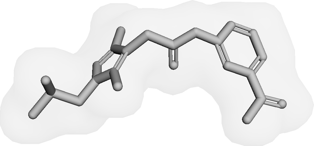
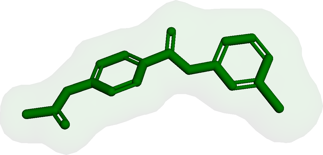
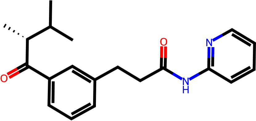
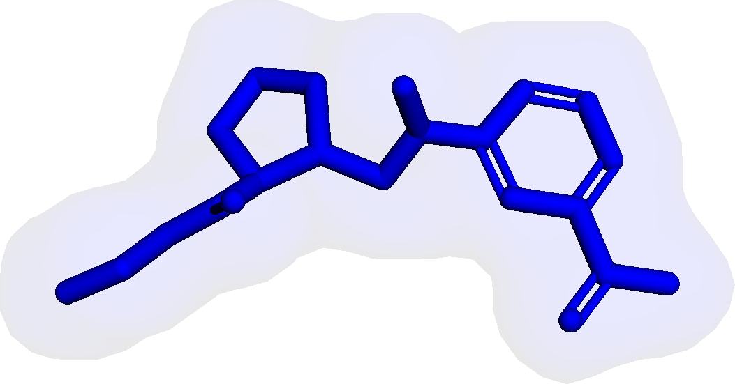
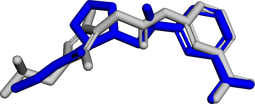
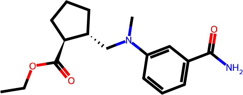
Case Study

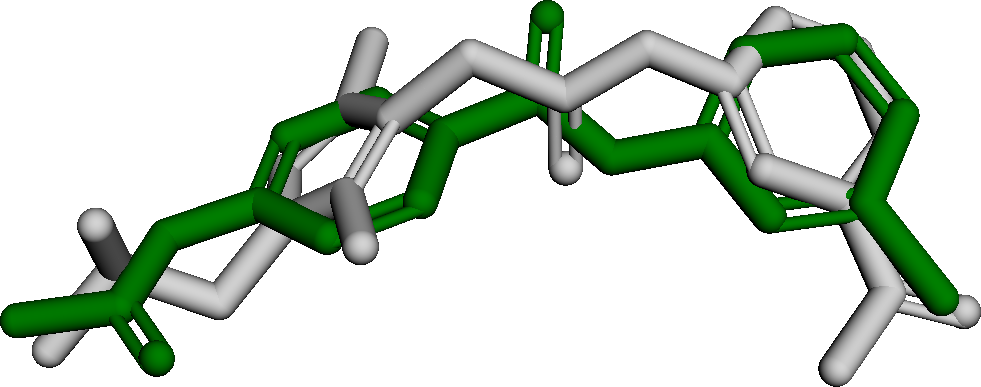
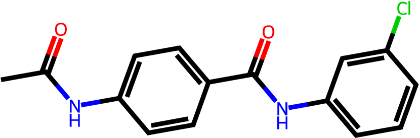
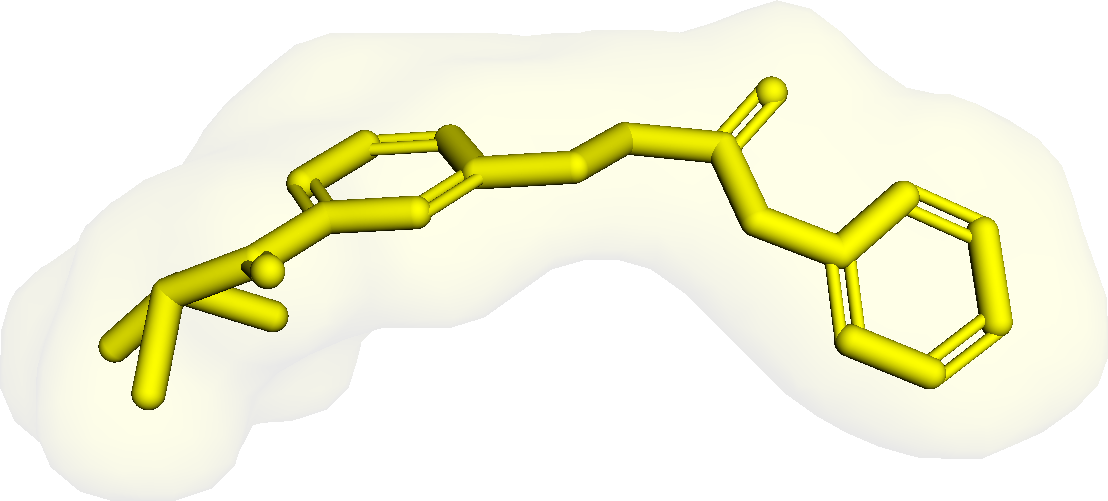
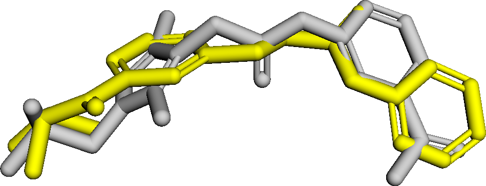
Figure 3 presents three generated molecules from three methods given the same condition molecule. As shown in Figure 3, the molecule generated by $\mathop{\mathsf{ShapeMol}}\limits$ has higher shape similarity (0.835) with the condition molecule than those from the baseline methods (0.759 for $\mathop{\mathsf{VS}}\limits$ and 0.749 for $\mathop{\mathsf{SQUID}}\limits$ ). Particularly, the molecule from $\mathop{\mathsf{ShapeMol}}\limits$ has the surface shape (represented as blue shade in Figure 3(d)) most similar to that of the condition molecule. All three molecules have low graph similarities with the condition molecule and higher $\mathop{\mathsf{QED}}\limits$ scores than the condition molecule. This example shows the ability of $\mathop{\mathsf{ShapeMol}}\limits$ to generate novel molecules that are more similar in 3D shape to condition molecules than those from baseline methods.

Discussions and Conclusions

In this paper, we develop a novel generative model $\mathop{\mathsf{ShapeMol}}\limits$ , which generates 3D molecules conditioned on the 3D shape of given molecules. $\mathop{\mathsf{ShapeMol}}\limits$ utilizes a pre-trained equivariant shape encoder to generate equivariant embeddings for 3D shapes of given molecules. Conditioned on the embeddings, $\mathop{\mathsf{ShapeMol}}\limits$ learns an equivariant diffusion model to generate novel molecules. To improve the shape similarities between the given molecule and the generated ones, we develop $\mathop{\mathsf{ShapeMol}\text{+}\mathsf{g}}\limits$ , which incorporates shape guidance to push the generated atom positions to the shape of the given molecule. We compare $\mathop{\mathsf{ShapeMol}}\limits$ and $\mathop{\mathsf{ShapeMol}\text{+}\mathsf{g}}\limits$ against state-of-the-art baseline methods. Our experimental results demonstrate that $\mathop{\mathsf{ShapeMol}}\limits$ and $\mathop{\mathsf{ShapeMol}\text{+}\mathsf{g}}\limits$ could generate molecules with higher shape similarities, and competitive qualities compared to the baseline methods. In future work, we will explore generating 3D molecules jointly conditioned on the shape and the electrostatic, considering that the electrostatic of molecules could also determine the binding activities of molecules.

Acknowledgements

This project was made possible, in part, by support from the National Science Foundation grant nos. IIS-2133650 (X.N.), and The Ohio State University President’s Research Excellence program (X.N.). Any opinions, findings and conclusions or recommendations expressed in this paper are those of the authors and do not necessarily reflect the views of the funding agency.

References

Acharya et al. (2011) Acharya, C.; Coop, A.; Polli, J. E.; and MacKerell, A. D. 2011. Recent Advances in Ligand-Based Drug Design: Relevance and Utility of the Conformationally Sampled Pharmacophore Approach. Current Computer Aided-Drug Design, 7(1): 10–22.
Adams and Coley (2023) Adams, K.; and Coley, C. W. 2023. Equivariant Shape-Conditioned Generation of 3D Molecules for Ligand-Based Drug Design. In The Eleventh International Conference on Learning Representations.
Batool, Ahmad, and Choi (2019) Batool, M.; Ahmad, B.; and Choi, S. 2019. A Structure-Based Drug Discovery Paradigm. International Journal of Molecular Sciences, 20(11): 2783.
Chen et al. (2022) Chen, Y.; Fernando, B.; Bilen, H.; Nießner, M.; and Gavves, E. 2022. 3D Equivariant Graph Implicit Functions. In Lecture Notes in Computer Science, 485–502. Springer Nature Switzerland.
Chen et al. (2021) Chen, Z.; Min, M. R.; Parthasarathy, S.; and Ning, X. 2021. A deep generative model for molecule optimization via one fragment modification. Nature Machine Intelligence, 3(12): 1040–1049.
Deng et al. (2021) Deng, C.; Litany, O.; Duan, Y.; Poulenard, A.; Tagliasacchi, A.; and Guibas, L. J. 2021. Vector Neurons: A General Framework for SO(3)-Equivariant Networks. In Proceedings of the IEEE/CVF International Conference on Computer Vision (ICCV), 12200–12209.
Garcia Satorras et al. (2021) Garcia Satorras, V.; Hoogeboom, E.; Fuchs, F.; Posner, I.; and Welling, M. 2021. E(n) Equivariant Normalizing Flows. In Ranzato, M.; Beygelzimer, A.; Dauphin, Y.; Liang, P.; and Vaughan, J. W., eds., Advances in Neural Information Processing Systems, volume 34, 4181–4192. Curran Associates, Inc.
Gómez-Bombarelli et al. (2018) Gómez-Bombarelli, R.; Wei, J. N.; Duvenaud, D.; Hernández-Lobato, J. M.; Sánchez-Lengeling, B.; Sheberla, D.; Aguilera-Iparraguirre, J.; Hirzel, T. D.; Adams, R. P.; and Aspuru-Guzik, A. 2018. Automatic Chemical Design Using a Data-Driven Continuous Representation of Molecules. ACS Central Science, 4(2): 268–276.
Guan et al. (2023) Guan, J.; Qian, W. W.; Peng, X.; Su, Y.; Peng, J.; and Ma, J. 2023. 3D Equivariant Diffusion for Target-Aware Molecule Generation and Affinity Prediction. In The Eleventh International Conference on Learning Representations.
Hawkins, Skillman, and Nicholls (2006) Hawkins, P. C. D.; Skillman, A. G.; and Nicholls, A. 2006. Comparison of Shape-Matching and Docking as Virtual Screening Tools. Journal of Medicinal Chemistry, 50(1): 74–82.
Ho, Jain, and Abbeel (2020) Ho, J.; Jain, A.; and Abbeel, P. 2020. Denoising Diffusion Probabilistic Models. In Larochelle, H.; Ranzato, M.; Hadsell, R.; Balcan, M.; and Lin, H., eds., Advances in Neural Information Processing Systems, volume 33, 6840–6851. Curran Associates, Inc.
Hoogeboom et al. (2021) Hoogeboom, E.; Nielsen, D.; Jaini, P.; Forré, P.; and Welling, M. 2021. Argmax Flows and Multinomial Diffusion: Learning Categorical Distributions. In Ranzato, M.; Beygelzimer, A.; Dauphin, Y.; Liang, P.; and Vaughan, J. W., eds., Advances in Neural Information Processing Systems, volume 34, 12454–12465. Curran Associates, Inc.
Hoogeboom et al. (2022) Hoogeboom, E.; Satorras, V. G.; Vignac, C.; and Welling, M. 2022. Equivariant Diffusion for Molecule Generation in 3D. In Chaudhuri, K.; Jegelka, S.; Song, L.; Szepesvari, C.; Niu, G.; and Sabato, S., eds., Proceedings of the 39th International Conference on Machine Learning, volume 162 of Proceedings of Machine Learning Research, 8867–8887. PMLR.
Imrie et al. (2021) Imrie, F.; Hadfield, T. E.; Bradley, A. R.; and Deane, C. M. 2021. Deep generative design with 3D pharmacophoric constraints. Chemical Science, 12(43): 14577–14589.
Jin, Barzilay, and Jaakkola (2018) Jin, W.; Barzilay, R.; and Jaakkola, T. 2018. Junction Tree Variational Autoencoder for Molecular Graph Generation. In Dy, J.; and Krause, A., eds., Proceedings of the 35th International Conference on Machine Learning, volume 80 of Proceedings of Machine Learning Research, 2323–2332. PMLR.
Kingma and Ba (2015) Kingma, D. P.; and Ba, J. 2015. Adam: A Method for Stochastic Optimization. In Bengio, Y.; and LeCun, Y., eds., 3rd International Conference on Learning Representations, ICLR 2015, San Diego, CA, USA, 2015.
Kong et al. (2021) Kong, Z.; Ping, W.; Huang, J.; Zhao, K.; and Catanzaro, B. 2021. DiffWave: A Versatile Diffusion Model for Audio Synthesis. In International Conference on Learning Representations.
Kullback and Leibler (1951) Kullback, S.; and Leibler, R. A. 1951. On Information and Sufficiency. The Annals of Mathematical Statistics, 22(1): 79–86.
Landrum et al. (2023) Landrum, G.; Tosco, P.; Kelley, B.; Ric; Cosgrove, D.; Sriniker; Gedeck; Vianello, R.; NadineSchneider; Kawashima, E.; N, D.; Jones, G.; Dalke, A.; Cole, B.; Swain, M.; Turk, S.; AlexanderSavelyev; Vaucher, A.; Wójcikowski, M.; Ichiru Take; Probst, D.; Ujihara, K.; Scalfani, V. F.; Godin, G.; Lehtivarjo, J.; Pahl, A.; Walker, R.; Francois Berenger; Jasondbiggs; and Strets123. 2023. rdkit/rdkit: 2023_03_2 (Q1 2023) Release.
Luo et al. (2021) Luo, S.; Guan, J.; Ma, J.; and Peng, J. 2021. A 3D Generative Model for Structure-Based Drug Design. In Beygelzimer, A.; Dauphin, Y.; Liang, P.; and Vaughan, J. W., eds., Advances in Neural Information Processing Systems.
Nichol and Dhariwal (2021) Nichol, A. Q.; and Dhariwal, P. 2021. Improved Denoising Diffusion Probabilistic Models. In Meila, M.; and Zhang, T., eds., Proceedings of the 38th International Conference on Machine Learning, volume 139 of Proceedings of Machine Learning Research, 8162–8171. PMLR.
Papadopoulos et al. (2021) Papadopoulos, K.; Giblin, K. A.; Janet, J. P.; Patronov, A.; and Engkvist, O. 2021. De novo design with deep generative models based on 3D similarity scoring. Bioorganic &amp: Medicinal Chemistry, 44: 116308.
Park et al. (2019) Park, J. J.; Florence, P.; Straub, J.; Newcombe, R.; and Lovegrove, S. 2019. DeepSDF: Learning Continuous Signed Distance Functions for Shape Representation. In Proceedings of the IEEE/CVF Conference on Computer Vision and Pattern Recognition (CVPR).
Peng et al. (2023) Peng, X.; Guan, J.; Liu, Q.; and Ma, J. 2023. MolDiff: Addressing the Atom-Bond Inconsistency Problem in 3D Molecule Diffusion Generation. In Krause, A.; Brunskill, E.; Cho, K.; Engelhardt, B.; Sabato, S.; and Scarlett, J., eds., Proceedings of the 40th International Conference on Machine Learning, volume 202 of Proceedings of Machine Learning Research, 27611–27629. PMLR.
Peng et al. (2022) Peng, X.; Luo, S.; Guan, J.; Xie, Q.; Peng, J.; and Ma, J. 2022. Pocket2Mol: Efficient Molecular Sampling Based on 3D Protein Pockets. In Chaudhuri, K.; Jegelka, S.; Song, L.; Szepesvari, C.; Niu, G.; and Sabato, S., eds., Proceedings of the 39th International Conference on Machine Learning, volume 162 of Proceedings of Machine Learning Research, 17644–17655. PMLR.
Polykovskiy et al. (2020) Polykovskiy, D.; Zhebrak, A.; Sanchez-Lengeling, B.; Golovanov, S.; Tatanov, O.; Belyaev, S.; Kurbanov, R.; Artamonov, A.; Aladinskiy, V.; Veselov, M.; Kadurin, A.; Johansson, S.; Chen, H.; Nikolenko, S.; Aspuru-Guzik, A.; and Zhavoronkov, A. 2020. Molecular Sets (MOSES): A Benchmarking Platform for Molecular Generation Models. Frontiers in Pharmacology, 11.
Ravi et al. (2020) Ravi, N.; Reizenstein, J.; Novotny, D.; Gordon, T.; Lo, W.-Y.; Johnson, J.; and Gkioxari, G. 2020. Accelerating 3D Deep Learning with PyTorch3D. arXiv:2007.08501.
Ripphausen, Nisius, and Bajorath (2011) Ripphausen, P.; Nisius, B.; and Bajorath, J. 2011. State-of-the-art in ligand-based virtual screening. Drug Discovery Today, 16(9-10): 372–376.
Vainio, Puranen, and Johnson (2009) Vainio, M. J.; Puranen, J. S.; and Johnson, M. S. 2009. ShaEP: Molecular Overlay Based on Shape and Electrostatic Potential. Journal of Chemical Information and Modeling, 49(2): 492–502.
Wang et al. (2019) Wang, Y.; Sun, Y.; Liu, Z.; Sarma, S. E.; Bronstein, M. M.; and Solomon, J. M. 2019. Dynamic Graph CNN for Learning on Point Clouds. ACM Trans. Graph., 38(5).
Wójcikowski, Zielenkiewicz, and Siedlecki (2015) Wójcikowski, M.; Zielenkiewicz, P.; and Siedlecki, P. 2015. Open Drug Discovery Toolkit (ODDT): a new open-source player in the drug discovery field. Journal of Cheminformatics, 7(1).
Zheng et al. (2013) Zheng, H.; Hou, J.; Zimmerman, M. D.; Wlodawer, A.; and Minor, W. 2013. The future of crystallography in drug discovery. Expert Opinion on Drug Discovery, 9(2): 125–137.

See pages - of supp.pdf

	$\displaystyle p(\mbox{$\mathop{\mathbf{x}}\limits$}_{t-1}\|\mbox{$\mathop{\mathbf{x}}\limits$}_{t})$	$\displaystyle\approx p_{\boldsymbol{\Theta}}(\mbox{$\mathop{\mathbf{x}}\limits$}_{t-1}\|\mbox{$\mathop{\mathbf{x}}\limits$}_{t},\tilde{\mbox{$\mathop{\mathbf{x}}\limits$}}_{0,t})$		(14)
		$\displaystyle=\mathcal{N}(\mbox{$\mathop{\mathbf{x}}\limits$}_{t-1}\|\mu_{\boldsymbol{\Theta}}(\mbox{$\mathop{\mathbf{x}}\limits$}_{t},\tilde{\mbox{$\mathop{\mathbf{x}}\limits$}}_{0,t}),\tilde{\beta}^{\mathtt{x}}_{t}\mathbf{I}),$		(14)

Shape-conditioned 3D Molecule Generation via Equivariant Diffusion Models

Abstract

Introduction

Related Work

Molecule Generation

Shape-Conditioned Molecule Generation

Definitions and Notations

Problem Definition

Representations and Notations

Method

Equivariant Shape Embedding (𝖲𝖤\mathop{\mathsf{SE}}\limits)

Shape Encoder (𝖲𝖤​-​𝖾𝗇𝖼\mathop{\mathsf{SE}\text{-}\mathsf{enc}}\limits)

Shape Decoder (𝖲𝖤​-​𝖽𝖾𝖼\mathop{\mathsf{SE}\text{-}\mathsf{dec}}\limits)

𝖲𝖤\mathop{\mathsf{SE}}\limits Pre-training

Shape-Conditioned Molecule Generation

Forward Diffusion Process (𝖣𝖨𝖥𝖥​-​𝖿𝗈𝗋𝗐𝖺𝗋𝖽\mathop{\mathsf{DIFF}\text{-}\mathsf{forward}}\limits)

Backward Generative Process (𝖣𝖨𝖥𝖥​-​𝖻𝖺𝖼𝗄𝗐𝖺𝗋𝖽\mathop{\mathsf{DIFF}\text{-}\mathsf{backward}}\limits)

Equivariant Shape-Conditioned Molecule Predictor

Atom Coordinate Prediction

Atom Feature Prediction

Model Training

Molecule Generation

𝖲𝗁𝖺𝗉𝖾𝖬𝗈𝗅\mathop{\mathsf{ShapeMol}}\limits with Shape Guidance

Experiments

Data

Baselines

Evaluation Metrics

Performance Comparison

Overall Comparison

Comparison of Diffusion Weighting Schemes

Parameter Study

Case Study

Discussions and Conclusions

Acknowledgements

References

Equivariant Shape Embedding ( $\mathop{\mathsf{SE}}\limits$ )

Shape Encoder ( $\mathop{\mathsf{SE}\text{-}\mathsf{enc}}\limits$ )

Shape Decoder ( $\mathop{\mathsf{SE}\text{-}\mathsf{dec}}\limits$ )

$\mathop{\mathsf{SE}}\limits$ Pre-training

Forward Diffusion Process ( $\mathop{\mathsf{DIFF}\text{-}\mathsf{forward}}\limits$ )

Backward Generative Process ( $\mathop{\mathsf{DIFF}\text{-}\mathsf{backward}}\limits$ )

$\mathop{\mathsf{ShapeMol}}\limits$ with Shape Guidance