Sharp oracle inequalities for aggregation of affine estimators
Abstract
We consider the problem of combining a (possibly uncountably infinite) set of affine estimators in nonparametric regression model with heteroscedastic Gaussian noise. Focusing on the exponentially weighted aggregate, we prove a PAC-Bayesian type inequality that leads to sharp oracle inequalities in discrete but also in continuous settings. The framework is general enough to cover the combinations of various procedures such as least square regression, kernel ridge regression, shrinking estimators and many other estimators used in the literature on statistical inverse problems. As a consequence, we show that the proposed aggregate provides an adaptive estimator in the exact minimax sense without discretizing the range of tuning parameters or splitting the set of observations. We also illustrate numerically the good performance achieved by the exponentially weighted aggregate.
doi:
10.1214/12-AOS1038keywords:
[class=AMS]keywords:
and T1Supported in part by ANR Parcimonie.
1 Introduction
There is growing empirical evidence of superiority of aggregated statistical procedures, also referred to as blending, stacked generalization or ensemble methods, with respect to “pure” ones. Since their introduction in the 1990s, famous aggregation procedures such as Boosting Freund90 , Bagging Breiman96b or Random Forest AmitGeman97 have been successfully used in practice for a large variety of applications. Moreover, most recent Machine Learning competitions such as the Pascal VOC or Netflix challenge have been won by procedures combining different types of classifiers/predictors/estimators. It is therefore of central interest to understand from a theoretical point of view what kind of aggregation strategies should be used for getting the best possible combination of the available statistical procedures.
1.1 Historical remarks and motivation
In the statistical literature, to the best of our knowledge, theoretical foundations of aggregation procedures were first studied by Nemirovski (Nemirovski Nemirovski00 , Juditsky and Nemirovski JuditskyNemirovski00 ) and independently by a series of papers by Catoni (see Catoni04 for an account) and Yang Yang00 , Yang03 , Yang04a . For the regression model, a significant progress was achieved by Tsybakov Tsybakov03 with introducing the notion of optimal rates of aggregation and proposing aggregation-rate-optimal procedures for the tasks of linear, convex and model selection aggregation. This point was further developed in Lounici07 , RigolletTsybakov07 , BuneaTsybakovWegkamp07 , especially in the context of high dimension with sparsity constraints and in Rigollet09 for Kullback–Leibler aggregation. However, it should be noted that the procedures proposed in Tsybakov03 that provably achieve the lower bounds in convex and linear aggregation require full knowledge of design distribution. This limitation was overcome in the recent work Wang2011 .
From a practical point of view, an important limitation of the previously cited results on aggregation is that they are valid under the assumption that the aggregated procedures are deterministic (or random, but independent of the data used for aggregation). The generality of those results—almost no restriction on the constituent estimators—compensates to this practical limitation.
In the Gaussian sequence model, a breakthrough was reached by Leung and Barron LeungBarron06 . Building on very elegant but not very well-known results by George George86a 222Corollary 2 in George86a coincides with Theorem 1 in LeungBarron06 in the case of exponential weights with temperature ; cf. equation (4) below for a precise definition of exponential weights. Furthermore, to the best of our knowledge, George86a is the first reference using the Stein lemma for evaluating the expected risk of the exponentially weighted aggregate., they established sharp oracle inequalities for the exponentially weighted aggregate (EWA) for constituent estimators obtained from the data vector by orthogonally projecting it on some linear subspaces. Dalalyan and Tsybakov DalalyanTsybakov07 , DalalyanTsybakov08 showed the result of LeungBarron06 remains valid under more general (non-Gaussian) noise distributions and when the constituent estimators are independent of the data used for the aggregation. A natural question arises whether a similar result can be proved for a larger family of constituent estimators containing projection estimators and deterministic ones as specific examples. The main aim of the present paper is to answer this question by considering families of affine estimators.
Our interest in affine estimators is motivated by several reasons. First, affine estimators encompass many popular estimators such as smoothing splines, the Pinsker estimator Pinsker80 , EfromovichPinsker96 , local polynomial estimators, nonlocal means BuadesCollMorel05 , SalmonLepennec09b , etc. For instance, it is known that if the underlying (unobserved) signal belongs to a Sobolev ball, then the (linear) Pinsker estimator is asymptotically minimax up to the optimal constant, while the best projection estimator is only rate-minimax. A second motivation is that—as proved by Juditsky and Nemirovski JuditskyNemirovski09 —the set of signals that are well estimated by linear estimators is very rich. It contains, for instance, sampled smooth functions, sampled modulated smooth functions and sampled harmonic functions. One can add to this set the family of piecewise constant functions as well, as demonstrated in PolzehlSpokoiny00 , with natural application in magnetic resonance imaging. It is worth noting that oracle inequalities for penalized empirical risk minimizer were also proved by Golubev Golubev10 , and for model selection by Arlot and Bach ArlotBach09 , Baraud, Giraud and Huet BaraudGiraudHuet10 .
In the present work, we establish sharp oracle inequalities in the model of heteroscedastic regression, under various conditions on the constituent estimators assumed to be affine functions of the data. Our results provide theoretical guarantees of optimality, in terms of expected loss, for the exponentially weighted aggregate. They have the advantage of covering in a unified fashion the particular cases of frozen estimators considered in DalalyanTsybakov08 and of projection estimators treated in LeungBarron06 .
We focus on the theoretical guarantees expressed in terms of oracle inequalities for the expected squared loss. Interestingly, although several recent papers ArlotBach09 , BaraudGiraudHuet10 , GoldenshlugerLepski08 discuss the paradigm of competing against the best linear procedure from a given family, none of them provide oracle inequalities with leading constant equal to one. Furthermore, most existing results involve some constants depending on different parameters of the setup. In contrast, the oracle inequality that we prove herein is with leading constant one and admits a simple formulation. It is established for (suitably symmetrized, if necessary) exponentially weighted aggregates George86a , Catoni04 , DalalyanTsybakov07 with an arbitrary prior and a temperature parameter which is not too small. The result is nonasymptotic but leads to an asymptotically optimal residual term when the sample size, as well as the cardinality of the family of constituent estimators, tends to infinity. In its general form, the residual term is similar to those obtained in the PAC-Bayes setting Mcallester98 , Langford02 , Seeger03 in that it is proportional to the Kullback–Leibler divergence between two probability distributions.
The problem of competing against the best procedure in a given family was extensively studied in the context of online learning and prediction with expert advice KivinenWarmuth99 , Cesa-BianchiLugosi06 . A connection between the results on online learning and statistical oracle inequalities was established by Gerchinovitz Gerchinovitz11 .
1.2 Notation and examples of linear estimators
Throughout this work, we focus on the heteroscedastic regression model with Gaussian additive noise. We assume we are given a vector obeying the model
| (1) |
where is a centered Gaussian random vector, where is an unknown function and are deterministic points. Here, no assumption is made on the set . Our objective is to recover the vector , often referred to as signal, based on the data . In our work, the noise covariance matrix is assumed to be finite with a known upper bound on its spectral norm . We denote by the empirical inner product in : . We measure the performance of an estimator by its expected empirical quadratic loss: where .
We only focus on the task of aggregating affine estimators indexed by some parameter . These estimators can be written as affine transforms of the data . Using the convention that all vectors are one-column matrices, we have , where the real matrix and the vector are deterministic. It means the entries of and may depend on the points but not on the data . Let us describe now different families of linear and affine estimators successfully used in the statistical literature. Our results apply to all these families, leading to a procedure that behaves nearly as well as the best (unknown) one of the family.
Ordinary least squares. Let be a set of linear subspaces of . A well-known family of affine estimators, successfully used in the context of model selection BarronBirgeMassart99 , is the set of orthogonal projections onto . In the case of a family of linear regression models with design matrices , one has , where stands for the Moore–Penrose pseudo-inverse of .
Diagonal filters. Other common estimators are the so-called diagonal filters corresponding to diagonal matrices . Examples include the following:
-
•
Ordered projections: for some integer [ is the indicator function]. Those weights are also called truncated SVD (Singular Value Decomposition) or spectral cutoff. In this case a natural parametrization is , indexing the number of elements conserved.
-
•
Block projections: , , where . Here the natural parametrization is , indexing subsets of .
-
•
Tikhonov–Philipps filter: , where . In this case, , indexing continuously the smoothing parameters.
-
•
Pinsker filter: , where and .
Kernel ridge regression. Assume that we have a positive definite kernel and we aim at estimating the true function in the associated reproducing kernel Hilbert space (). The kernel ridge estimator is obtained by minimizing the criterion w.r.t. (see Shawe-TaylorChristianini00 , page 118). Denoting by the kernel-matrix with element , the unique solution is a linear estimate of the data, , with , where is the identity matrix.
Multiple Kernel learning. As described in ArlotBach09 , it is possible to handle the case of several kernels , with associated positive definite matrices . For a parameter , one can define the estimators with
| (2) |
It is worth mentioning that the formulation in equation (2) can be linked to the group Lasso YuanLin06 and to the multiple kernel learning introduced in LanckrietCristianiniBartlettElGhaouiJordan03 —see ArlotBach09 for more details.
Moving averages. If we think of coordinates of as some values assigned to the vertices of an undirected graph, satisfying the property that two nodes are connected if the corresponding values of are close, then it is natural to estimate by averaging out the values for indices that are connected to . The resulting estimator is a linear one with a matrix such that , where is the set of neighbors of the node in the graph and is the cardinality of .
1.3 Organization of the paper
In Section 2 we introduce EWA and state a PAC-Bayes type bound in expectation assessing optimality properties of EWA in combining affine estimators. The strengths and limitations of the results are discussed in Section 3. The extension of these results to the case of grouped aggregation—in relation with ill-posed inverse problems—is developed in Section 4. As a consequence, we provide in Section 5 sharp oracle inequalities in various setups: ranging from finite to continuous families of constituent estimators and including sparse scenarii. In Section 6 we apply our main results to prove that combining Pinsker’s type filters with EWA leads to asymptotically sharp adaptive procedures over Sobolev ellipsoids. Section 7 is devoted to numerical comparison of EWA with other classical filters (soft thresholding, blockwise shrinking, etc.) and illustrates the potential benefits of aggregating. The conclusion is given in Section 8, while the proofs of some technical results (Propositions 2–6) are provided in the supplementary material DalalyanSalmonsupp .
2 Aggregation of estimators: Main results
In this section we describe the statistical framework for aggregating estimators and we introduce the exponentially weighted aggregate. The task of aggregation consists in estimating by a suitable combination of the elements of a family of constituent estimators . The target objective of the aggregation is to build an aggregate that mimics the performance of the best constituent estimator, called oracle (because of its dependence on the unknown function ). In what follows, we assume that is a measurable subset of , for some .
The theoretical tool commonly used for evaluating the quality of an aggregation procedure is the oracle inequality (OI), generally written
| (3) |
with residual term tending to zero as , and leading constant being bounded. The OIs with leading constant one are of central theoretical interest since they allow to bound the excess risk and to assess the aggregation-rate-optimality. They are often referred to as sharp OI.
2.1 Exponentially weighted aggregate (EWA)
Let denote the risk of the estimator , for any , and let be an estimator of . The precise form of strongly depends on the nature of the constituent estimators. For any probability distribution over and for any , we define the probability measure of exponential weights, , by
| (4) |
The corresponding exponentially weighted aggregate, henceforth denoted by , is the expectation of w.r.t. the probability measure :
| (5) |
We will frequently use the terminology of Bayesian statistics: the measure is called prior, the measure is called posterior and the aggregate is then the posterior mean. The parameter will be referred to as the temperature parameter. In the framework of aggregating statistical procedures, the use of such an aggregate can be traced back to George George86a .
The interpretation of the weights is simple: they up-weight estimators all the more that their performance, measured in terms of the risk estimate , is good. The temperature parameter reflects the confidence we have in this criterion: if the temperature is small (), the distribution concentrates on the estimators achieving the smallest value for , assigning almost zero weights to the other estimators. On the other hand, if , then the probability distribution over is simply the prior , and the data do not influence our confidence in the estimators.
2.2 Main results
In this paper we only focus on affine estimators
| (6) |
where the real matrix and the vector are deterministic. Furthermore, we will assume that an unbiased estimator of the noise covariance matrix is available. It is well known (cf. Appendix for details) that the risk of the estimator (6) is given by
| (7) |
and that , defined by
| (8) |
is an unbiased estimator of . Along with , we will use another estimator of the risk that we call the adjusted risk estimate and define by
| (9) |
One can notice that the adjusted risk estimate coincides with the unbiased risk estimate if and only if the matrix is an orthogonal projector.
To state our main results, we denote by the set of all probability measures on and by the Kullback–Leibler divergence between two probability measures :
We write (resp., ) for two symmetric matrices and , when (resp., ) is semi-definite positive.
Theorem 1
Let all the matrices be symmetric and be unbiased and independent of . {longlist}[(ii)]
The simplest setting in which all the conditions of part (i) of Theorem 1 are fulfilled is when the matrices and are all diagonal, or diagonalizable in a common base. This result, as we will see in Section 6, leads to a new estimator which is adaptive, in the exact minimax sense, over the collection of all Sobolev ellipsoids. It also suggests a new method for efficiently combining varying-block-shrinkage estimators, as described in Section 5.4.
However, part (i) of Theorem 1 leaves open the issue of aggregating affine estimators defined via noncommuting matrices. In particular, it does not allow us to evaluate the MSE of EWA when each is a convex or linear combination of a fixed family of projection matrices on nonorthogonal linear subspaces. These kinds of situations may be handled via the result of part (ii) of Theorem 1. One can observe that in the particular case of a finite collection of projection estimators (i.e., and for every ), the result of part (ii) offers an extension of LeungBarron06 , Corollary 6, to the case of general noise covariances (LeungBarron06 deals only with i.i.d. noise).
An important situation covered by part (ii) of Theorem 1, but not by part (i), concerns the case when signals of interest are smooth or sparse in a basis which is different from the basis orthogonalizing the covariance matrix . In such a context, one may be interested in considering matrices that are diagonalizable in the basis which, in general, do not commute with .
Remark 1.
While the results in LeungBarron06 yield a sharp oracle inequality in the case of projection matrices , they are of no help in the case when the matrices are nearly idempotent and not exactly. Assertion (ii) of Theorem 1 fills this gap by showing that if , then is bounded by
Remark 2.
We have focused only on Gaussian errors to emphasize that it is possible to efficiently aggregate almost any family of affine estimators. We believe that by a suitable adaptation of the approach developed in DalalyanTsybakov08 , claims of Theorem 1 can be generalized—at least when are independent with known variances—to some other common noise distributions.
The results presented so far concern the situation when the matrices are symmetric. However, using the last part of Theorem 1, it is possible to propose an estimator of that is almost as accurate as the best affine estimator even if the matrices are not symmetric. Interestingly, the estimator enjoying this property is not obtained by aggregating the original estimators but the “symmetrized” estimators , where . Besides symmetry, an advantage of the matrices , as compared to the ’s, is that they automatically satisfy the contraction condition required by part (ii) of Theorem 1. We will refer to this method as Symmetrized Exponentially Weighted Aggregates (or SEWA) DalalyanSalmon11b .
Theorem 2
Assume that the matrices and the vectors satisfy for every . Assume in addition that is an unbiased estimator of and is independent of . Let denote the exponentially weighted aggregate of the (symmetrized) estimators with the weights (4) defined via the risk estimate . Then, under the conditions and
| (C) |
it holds that
| (2.9) |
To understand the scope of condition (C), let us present several cases of widely used linear estimators for which this condition is satisfied:
-
•
The simplest class of matrices for which condition (C) holds true are orthogonal projections. Indeed, if is a projection matrix, it satisfies and, therefore, .
- •
-
•
Under a little bit more stringent assumption of homoscedasticity, that is, when , if the matrices are such that all the nonzero elements of each row are equal and sum up to one (or a quantity larger than one), then and (C) is fulfilled. A notable example of linear estimators that satisfy this condition are Nadaraya–Watson estimators with rectangular kernel and nearest neighbor filters.
3 Discussion
Before elaborating on the main results stated in the previous section, by extending them to inverse problems and by deriving adaptive procedures, let us discuss some aspects of the presented OIs.
3.1 Assumptions on
In some rare situations, the matrix is known and it is natural to use as an unbiased estimator. Besides this not very realistic situation, there are at least two contexts in which it is reasonable to assume that an unbiased estimator of , independent of , is available.
The first case corresponds to problems in which a signal can be recorded several times by the same device, or once but by several identical devices. For instance, this is the case when an object is photographed many times by the same digital camera during a short time period. Let be the available signals, which can be considered as i.i.d. copies of an -dimensional Gaussian vector with mean and covariance matrix . Then, defining and , we find ourselves within the framework covered by previous theorems. Indeed, with and is an unbiased estimate of , independent of . Note that our theory applies in this setting for every integer .
The second case is when the dominating part of the noise comes from the device which is used for recording the signal. In this case, the practitioner can use the device in order to record a known signal, . In digital image processing, can be a black picture. This will provide a noisy signal drawn from Gaussian distribution , independent of which is the signal of interest. Setting , one ends up with an unbiased estimator of , which is independent of .
3.2 OI in expectation versus OI with high probability
All the results stated in this work provide sharp nonasymptotic bounds on the expected risk of EWA. It would be insightful to complement this study by risk bounds that hold true with high probability. However, it was recently proved in DaiRigZha12 that EWA is deviation suboptimal: there exist a family of constituent estimators and a constant such that the difference between the risk of EWA and that of the best constituent estimator is larger than with probability at least . Nevertheless, several empirical studies (see, e.g., DaiZhang11 ) demonstrated that EWA has often a smaller risk than some of its competitors, such as the empirical star procedure Audibert07 , which are provably optimal in the sense of OIs with high probability. Furthermore, numerical experiments carried out in Section 7 show that the standard-deviation of the risk of EWA is of the order of . This suggests that under some conditions on the constituent estimators it might be possible to establish OIs for EWA that are similar to (10) but hold true with high probability. A step in proving this kind of result was done in LecueMendelson10 , Theorem C, for the model of regression with random design.
3.3 Relation to previous work and limits of our results
The OI of the previous section requires various conditions on the constituent estimators . One may wonder how general these conditions are and is it possible to extend these OIs to more general ’s. Although this work does not answer this question, we can sketch some elements of response.
First of all, we stress that the conditions of the present paper relax significantly those of previous results existing in statistical literature. For instance, Kneip Kneip94 considered only linear estimators, that is, and, more importantly, only ordered sets of commuting matrices . The ordering assumption is dropped in Leung and Barron LeungBarron06 , in the case of projection matrices. Note that neither of these assumptions is satisfied for the families of Pinsker and Tikhonov–Philipps estimators. The present work strengthens existing results in considering more general, affine estimators extending both projection matrices and ordered commuting matrices.
Despite the advances achieved in this work, there are still interesting cases that are not covered by our theory. We now introduce a family of estimators commonly used in image processing that do not satisfy our assumptions. In recent years, nonlocal means (NLM) became quite popular in image processing BuadesCollMorel05 . This method of signal denoising, shown to be tied in with EWA SalmonLepennec09b , removes noise by exploiting signals self-similarities. We briefly define the NLM procedure in the case of one-dimensional signals.
Assume that a vector given by (1) is observed with , , for some function . For a fixed “patch-size” , let us define and for every . The vectors and are, respectively, called true patch and noisy patch. The NLM consists in regarding the noisy patches as constituent estimators for estimating the true patch by applying EWA. One easily checks that the constituent estimators are affine in , that is, with and independent of . Indeed, if the distance between and is larger than , then is independent of and, therefore, and . If , then the matrix is a suitably chosen shift matrix and is the projection of onto the orthogonal complement of the image of . Unfortunately, these matrices and vectors do not fit our framework, that is, the assumption is not satisfied.
Finally, our proof technique is specific to affine estimators. Its extension to estimators defined as a more complex function of the data will certainly require additional tools and is a challenging problem for future research. Yet, it seems unlikely to get sharp OIs with optimal remainder term for a fairly general family of constituent estimators (without data-splitting), since this generality inherently increases the risk of overfitting.
4 Ill-posed inverse problems and group-weighting
As explained in CavalierGolubevPicardTsybakov02 , Cavalier08 , the model of heteroscedastic regression is well suited for describing inverse problems. In fact, let be a known linear operator on some Hilbert space , with inner product . For some , let be the random process indexed by such that
| (10) |
where is the noise magnitude and is a white Gaussian noise on , that is, for any the vector is Gaussian with zero mean and covariance matrix . The problem is then the following: estimate the element assuming the value of can be measured for any given . It is customary to use as the eigenvectors of the adjoint of . Under the condition that the operator is compact, the SVD yields and , for , where are the singular values, is an orthonormal basis in and is the corresponding orthonormal basis in . In view of (10), it holds that
| (11) |
Since in practice only a finite number of measurements can be computed, it is natural to assume that the values are available only for smaller than some integer . Under the assumption that , the last equation is equivalent to (1) with and for . Examples of inverse problems to which this statistical model has been successfully applied are derivative estimation, deconvolution with known kernel, computerized tomography—see Cavalier08 and the references therein for more applications.
For very mildly ill-posed inverse problems, that is, when the singular values of tend to zero not faster than any negative power of , the approach presented in Section 2 will lead to satisfactory results. Indeed, by choosing or , the remainder term in (10) and (2.9) becomes—up to a logarithmic factor—proportional to , which is the optimal rate in the case of very mild ill-posedness.
However, even for mildly ill-posed inverse problems, the approach developed in the previous section becomes obsolete since the remainder blows up when increases to infinity. Furthermore, this is not an artifact of our theoretical results, but rather a drawback of the aggregation strategy adopted in the previous section. Indeed, the posterior probability measure defined by (4) can be seen as the solution of the entropy-penalized empirical risk minimization problem:
| (12) |
where the is taken over the set of all probability distributions. It means the same regularization parameter is employed for estimating both the coefficients corrupted by noise of small magnitude and those corrupted by large noise. Since we place ourselves in the setting of known operator and, therefore, known noise levels, such a uniform treatment of all coefficients is unreasonable. It is more natural to upweight the regularization term in the case of large noise downweighting the data fidelity term and, conversely, to downweight the regularization in the case of small noise. This motivates our interest in the grouped EWA (or GEWA).
Let us consider a partition of the set : , for some integers . To each element of this partition, we associate the data sub-vector and the sub-vector of true function . As in previous sections, we are concerned by the aggregation of affine estimators , but here we will assume the matrices are block-diagonal:
Similarly, we define and as the sub-vectors of and , respectively, corresponding to the indices belonging to . We will also assume that the noise covariance matrix and its unbiased estimate are block-diagonal with blocks and , respectively. This notation implies, in particular, that for every . Moreover, the unbiased risk estimate of can be decomposed into the sum of unbiased risk estimates of , namely, , where
To state the analogues of Theorems 1 and 2, we introduce the following settings. {longlist}
For all and , are symmetric and satisfy , and . For a temperature vector and a prior , we define GEWA as , where with
| (13) |
For every and for every belonging to a set of -measure one, the matrices satisfy a.s. the inequality while the vectors are such that . In this case, for a temperature vector and a prior , we define GEWA as , where and is defined by (13). Note that this setting is the grouped version of the SEWA.
Theorem 3
Assume that is unbiased and independent of . Under setting 1, if for all , then
| (14) |
Under setting 2, this inequality holds true if for every .
As we shall see in Section 6, this theorem allows us to propose an estimator of the unknown signal which is adaptive w.r.t. the smoothness properties of the underlying signal and achieves the minimax rates and constants over the Sobolev ellipsoids provided that the operator is mildly ill-posed, that is, its singular values decrease at most polynomially.
5 Examples of sharp oracle inequalities
In this section we discuss consequences of the main result for specific choices of prior measures. For conveying the main messages of this section it is enough to focus on settings 1 and 2 in the case of only one group ().
5.1 Discrete oracle inequality
In order to demonstrate that inequality (14) can be reformulated in terms of an OI as defined by (3), let us consider the case when the prior is discrete, that is, for a countable set , and w.l.o.g . Then, the following result holds true.
Proposition 1.
Let be unbiased, independent of and be supported by . Under setting 1 with and , the aggregate satisfies the inequality
| (15) |
Furthermore, (15) holds true under setting 2 for .
It suffices to apply Theorem 3 and to upper-bound the right-hand side by the minimum over all Dirac measures such that . This inequality can be compared to Corollary 2 in BaraudGiraudHuet10 , Section 4.3. Our result has the advantage of having factor one in front of the expectation of the left-hand side, while in BaraudGiraudHuet10 a constant much larger than 1 appears. However, it should be noted that the assumptions on the (estimated) noise covariance matrix are much weaker in BaraudGiraudHuet10 .
5.2 Continuous oracle inequality
It may be useful in practice to combine a family of affine estimators indexed by an open subset of for some (e.g., to build an estimator nearly as accurate as the best kernel estimator with fixed kernel and varying bandwidth). To state an oracle inequality in such a “continuous” setup, let us denote by the largest real such that the ball centered at of radius —hereafter denoted by —is included in . Let be the Lebesgue measure in .
Proposition 2.
Let be unbiased, independent of . Let be an open and bounded set and let be the uniform distribution on . Assume that the mapping is Lipschitz continuous, that is, , . Under setting 1 with and , the aggregate satisfies the inequality
Furthermore, (2) holds true under setting 2 for every .
It suffices to apply assertion (i) of Theorem 1 and to upper-bound the right-hand side in inequality (10) by the minimum over all measures having as density . Choosing such that , the measure is absolutely continuous w.r.t. the uniform prior and the Kullback–Leibler divergence between these two measures equals . Using and the Lipschitz condition, we get the desired inequality.
Note that it is not very stringent to require the risk function to be Lipschitz continuous, especially since this condition needs not be satisfied uniformly in . Let us consider the ridge regression: for a given design matrix , and with , being a given normalization factor typically set to or , and . One can easily check the Lipschitz property of the risk function with .
5.3 Sparsity oracle inequality
The continuous oracle inequality stated in the previous subsection is well adapted to the problems in which the dimension of is small w.r.t. the sample size (or, more precisely, the signal to noise ratio ). When this is not the case, the choice of the prior should be done more carefully. For instance, consider with large under the sparsity scenario: there is a sparse vector such that the risk of is small. Then, it is natural to choose a prior that favors sparse ’s. This can be done in the same vein as in DalalyanTsybakov07 , DalalyanTsybakov08 , DalalyanTsybakov12a , DalalyanTsybakov12b , by means of the heavy tailed prior,
| (17) |
where is a tuning parameter.
Proposition 3.
Let us discuss here some consequences of this sparsity oracle inequality. First of all, consider the case of (linearly) combining frozen estimators, that is, when with some known functions . Then, it is clear that , where is the Gram matrix defined by . So the condition in Proposition 3 consists in bounding the Gram matrix of the atoms . Let us remark that in this case—see, for instance, DalalyanTsybakov08 , DalalyanTsybakov12b — is on the order of and the choice ensures that the last term in the right-hand side of equation (3) decreases at the parametric rate . This is the choice we recommend for practical applications.
As a second example, let us consider the case of a large number of linear estimators satisfying conditions of setting 1 and such that . Assume we aim at proposing an estimator mimicking the behavior of the best possible convex combination of a pair of estimators chosen among . This task can be accomplished in our framework by setting and , where . Remark that if satisfies conditions of setting 1, so does . Moreover, the mapping is quadratic with Hessian matrix given by the entries , . It implies that inequality (18) holds with . Therefore, denoting by the th diagonal entry of and setting , we get . Applying Proposition 3 with , we get
where the is taken over all and . This inequality is derived from (3) by upper-bounding the by the infimum over ’s having at most two nonzero coefficients, and , that are nonnegative and sum to one: . To get (5.3), one simply notes that only two terms of the sum are nonzero and each of them is not larger than . Thus, one can achieve using EWA the best possible risk over the convex combinations of a pair of linear estimators—selected from a large (but finite) family—at the price of a residual term that decreases at the parametric rate up to a log factor.
5.4 Oracle inequalities for varying-block-shrinkage estimators
Let us consider now the problem of aggregation of two-block shrinkage estimators. This means that the constituent estimators have the following form: for , where . Let us choose the prior as uniform on .
Proposition 4.
Let be the exponentially weighted aggregate having as constituent estimators two-block shrinkage estimators . If is diagonal, then for any and for any ,
| (21) |
In the case , this result is comparable to Leung , page 20, Theorem 2.49, which states that in the homoscedastic regression model (), EWA acting on two-block positive-part James–Stein estimators satisfies, for any such that and for , the oracle inequality
| (22) |
6 Application to minimax adaptive estimation
Pinsker proved in his celebrated paper Pinsker80 that in the model (1) the minimax risk over ellipsoids can be asymptotically attained by a linear estimator. Let us denote by the coefficients of the (orthogonal) discrete cosine333The results of this section hold true not only for the discrete cosine transform, but also for any linear transform such that . (DCT) transform of , hereafter denoted by . Pinsker’s result—restricted to Sobolev ellipsoids — states that, as , the equivalences
| (23) | |||||
| (24) |
hold Tsybakov09 , Theorem 3.2, where the first is taken over all possible estimators and is the Pinsker filter in the discrete cosine basis. In simple words, this implies that the (asymptotically) minimax estimator can be chosen from the quite narrow class of linear estimators with Pinsker’s filter. However, it should be emphasized that the minimax linear estimator depends on the parameters and , that are generally unknown. An (adaptive) estimator, that does not depend on and is asymptotically minimax over a large scale of Sobolev ellipsoids, has been proposed by Efromovich and Pinsker EfromovichPinsker84 . The next result, that is, a direct consequence of Theorem 1, shows that EWA with linear constituent estimators is also asymptotically sharp adaptive over Sobolev ellipsoids.
Proposition 5.
Let and consider the prior
| (25) |
where . Then, in model (1) with homoscedastic errors, the aggregate based on the temperature and the constituent estimators (with being the Pinsker filter) is adaptive in the exact minimax sense444See Tsybakov09 , Definition 3.8. on the family of classes .
It is worth noting that the exact minimax adaptivity property of our estimator is achieved without any tuning parameter. All previously proposed methods that are provably adaptive in an exact minimax sense depend on some parameters such as the lengths of blocks for blockwise Stein CavalierTsybakov02 and Efromovich–Pinsker EfromovichPinsker96 estimators or the step of discretization and the maximal value of bandwidth CavalierGolubevPicardTsybakov02 . Another nice property of the estimator is that it does not require any pilot estimator based on the data splitting device GaiffasLecue11 .
We now turn to the setup of heteroscedastic regression, which corresponds to ill-posed inverse problems as described in Section 4. To achieve adaptivity in the exact minimax sense, we make use of , the grouped version of the exponentially weighted aggregate. We assume hereafter that the matrix is diagonal with diagonal entries satisfying the following property:
| (26) |
This kind of problems arises when is a differential operator or the Radon transform Cavalier08 , Section 1.3. To handle such situations, we define the groups in the same spirit as the weakly geometrically increasing blocks in CavalierTsybakov01 . Let be a positive integer that increases as . Set and define
| (27) |
where stands for the largest integer strictly smaller than . Let be the smallest integer such that . We redefine and set for all .
Proposition 6.
Let the groups be defined as above with satisfying and as . Let and consider the prior
| (28) |
Then, in model (1) with diagonal covariance matrix satisfying condition (26), the aggregate (under setting 1) based on the temperatures and the constituent estimators (with being the Pinsker filter) is adaptive in the exact minimax sense on the family of classes .
Note that this result provides an estimator attaining the optimal constant in the minimax sense when the unknown signal lies in an ellipsoid. This property holds because minimax estimators over the ellipsoids are linear. For other subsets of , such as hyper-rectangles, Besov bodies and so on, this is not true anymore. However, as proved by Donoho, Liu and MacGibbon DonohoLiuMacGibbon90 , for orthosymmetric quadratically convex sets the minimax linear estimators have a risk which is within of the minimax risk among all estimates. Therefore, following the approach developed here, it is also possible to prove that GEWA can lead to an adaptive estimator whose risk is within of the minimax risk, for a broad class of hyperrectangles.
7 Experiments
In this section we present some numerical experiments on synthetic data, by focusing only on the case of homoscedastic Gaussian noise () with known variance. A toolbox is made available freely for download at http://josephsalmon.eu/code/index_codes.php. Additional details and numerical experiments can be found in DalalyanSalmon11b , SalmonDalalyan11c .
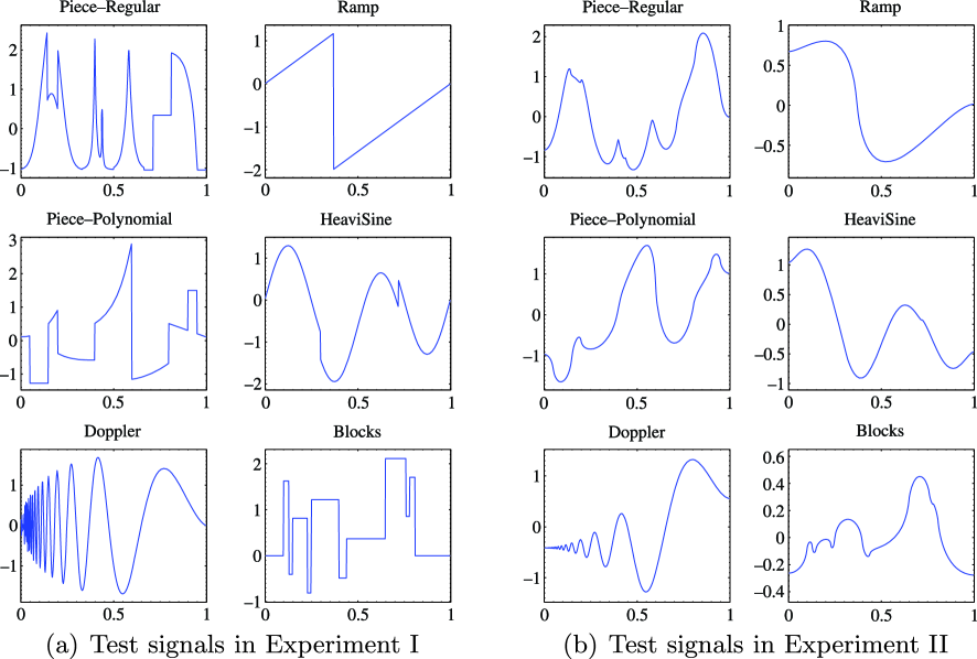
We evaluate different estimation routines on several 1D signals considered as a benchmark in the literature on signal processing DonohoJohnstone94 . The six signals we retained for our experiments because of their diversity are depicted in Figure 1. Since these signals are nonsmooth, we have also carried out experiments on their smoothed versions obtained by taking the antiderivative. Experiments on nonsmooth (resp., smooth) signals are referred to as Experiment I (resp., Experiment II). In both cases, prior to applying estimation routines, we normalize the (true) sampled signal to have an empirical norm equal to one and use the DCT denoted by .
The four tested estimation routines—including EWA—are detailed below.
Soft-Thresholding (ST) DonohoJohnstone94 : For a given shrinkage parameter , the soft-thresholding estimator is . We use the data-driven threshold minimizing the Stein unbiased risk estimate DonohoJohnstone95 .
Blockwise James–Stein (BJS) shrinkage Cai99 : The set is partitioned into blocks of nearly equal size . The corresponding blocks of true coefficients are then estimated by , with blocks of noisy coefficients , and .
Unbiased risk estimate (URE) minimization with Pinsker’s filters CavalierGolubevPicardTsybakov02 : Pinsker filter with data-driven parameters and selected by minimizing an unbiased estimate of the risk over a suitably chosen grid for the values of and . Here, we use geometric grids ranging from to for and from to for .
EWA on Pinsker’s filters: We consider the same finite family of linear filters (defined by Pinsker’s filters) as in the URE routine described above. According to Proposition 1, this leads to an estimator nearly as accurate as the best Pinsker’s estimator in the given family.
To report the result of our experiments, we have also computed the best linear smoother, hereafter referred to as the oracle, based on a Pinsker filter chosen among the candidates that we used for defining URE and EWA. By best smoother we mean the one minimizing the squared error (it can be computed since we know the ground truth). Results summarized in Table 1 for Experiment I and Table 2 for Experiment II correspond to the average over 1000 trials of the mean squared error (MSE) from which we subtract the MSE of the oracle and multiply the resulting difference by the sample size. We report the results for and for .
Simulations show that EWA and URE have very comparable performances and are significantly more accurate than soft-thresholding and block James–Stein (cf. Table 1) for every size of signals considered. Improvements are particularly important when signals have large peaks or discontinuities. In most cases, EWA also outperforms URE, but differences are less pronounced. One can also observe that for smooth signals, the difference of MSEs between EWA and the oracle, multiplied by , remains nearly constant when varies. This is in agreement with our theoretical results in which the residual term decreases to zero inversely proportionally to .
Of course, soft-thresholding and blockwise James–Stein procedures have been designed for being applied to the wavelet transform of a Besov smooth function, rather than to the Fourier transform of a Sobolev-smooth function. However, the point here is not to demonstrate the superiority of EWA as compared to ST and BJS procedures. The point is to stress the importance of having sharp adaptivity up to an optimal constant and not simply adaptivity in the sense of rate of convergence. Indeed, the procedures ST and BJS are provably rate-adaptive when applied to the Fourier transform of a Sobolev-smooth function, but they are not sharp adaptive—they do not attain the optimal constant—whereas EWA and URE do attain.
| EWA | URE | BJS | ST | EWA | URE | BJS | ST | ||
| Blocks | Doppler | ||||||||
| 256 | |||||||||
| 512 | |||||||||
| 1024 | |||||||||
| 2048 | |||||||||
| HeaviSine | Piece-Regular | ||||||||
| 256 | |||||||||
| 512 | |||||||||
| 1024 | |||||||||
| 2048 | |||||||||
| Ramp | Piece-Polynomial | ||||||||
| 256 | |||||||||
| 512 | |||||||||
| 1024 | |||||||||
| 2048 | |||||||||
8 Summary and future work
In this paper we have addressed the problem of aggregating a set of affine estimators in the context of regression with fixed design and heteroscedastic noise. Under some assumptions on the constituent estimators, we have proven that EWA with a suitably chosen temperature parameter satisfies PAC-Bayesian type inequality, from which different types of oracle inequalities have been deduced. All these inequalities are with leading constant one and rate-optimal residual term. As an application of our results, we have shown that EWA acting on Pinsker’s estimators produces an adaptive estimator in the exact minimax sense.
Next in our agenda is carrying out an experimental evaluation of the proposed aggregate using the approximation schemes described by Dalalyan and Tsybakov DalalyanTsybakov12b , Rigollet and Tsybakov RigolletTsybakov11 , RigolletTsybakov11b and Alquier and Lounici AlquierLounici10 , with a special focus on the problems involving large scale data.
Although we do not assume the covariance matrix of the noise to be known, our approach relies on an unbiased estimator of which is independent on the observed signal and on an upper bound on the largest singular value of . In some applications, such information may be hard to obtain and it can be helpful to relax the assumptions on . This is another interesting avenue for future research for which, we believe, the approach developed by Giraud Giraud08 can be of valuable guidance.
Appendix: Proofs of main theorems
We develop now the detailed proofs of the results stated in the manuscript.
.1 Stein’s lemma
The proofs of our main results rely on Stein’s lemma Stein73 , recalled below, providing an unbiased risk estimate for any estimator that depends sufficiently smoothly on the data vector .
Lemma 1.
Let be a random vector drawn form the Gaussian distribution . If the estimator is a.e. differentiable in and the elements of the matrix have finite first moment, then
is an unbiased estimate of , that is, .
The proof can be found in Tsybakov09 , page 157. We apply Stein’s lemma to the affine estimators , with an deterministic real matrix and a deterministic vector. We get that if is an unbiased estimator of , then is an unbiased estimator of the risk .
.2 An auxiliary result
Prior to proceeding with the proof of the main theorems, we prove an important auxiliary result which is the central ingredient of the proofs for our main results.
Lemma 2.
Let assumptions of Lemma 1 be satisfied. Let be a family of estimators of and a family of risk estimates such that the mapping is a.e. differentiable for every . Let be the unbiased risk estimate of given by Stein’s lemma. {longlist}[(1)]
For every and for any , the estimator defined as the average of w.r.t. to the probability measure
admits
as unbiased estimator of the risk.
If, furthermore, , and for some constant , then for every it holds that
| (29) |
According to the Stein lemma, the quantity
| (30) |
is an unbiased estimate of the risk . Using simple algebra, one checks that
| (31) |
By interchanging the integral and differential operators, we get the following relation: .Then, combining this equality with equations (30) and (31) implies that
After having interchanged differentiation and integration, we obtain that and, therefore, we come up with the following expression for :
This completes the proof of the first assertion of the lemma.
To prove the second assertion, let us observe that under the required condition and in view of the first assertion, for every it holds that . To conclude, it suffices to remark that is the probability measure minimizing the criterion among all . Thus, for every , we have
Taking the expectation of both sides, the desired result follows.
.3 Proof of Theorem 1
Assertion (i). In what follows, we use the matrix shorthand and . We apply Lemma 2 with . To check the conditions of the second part of Lemma 2, note that in view of equations (6) and (8), as well as the assumptions and , we get
Recall now that for any pair of commuting matrices and the identity holds true. Applying this identity to and (in view of the commuting property of the ’s), we get the following relation: . When one integrates over with respect to the measure , the term of the first scalar product in the right-hand side of the last equation vanishes. On the other hand,
Since positive semi-definiteness of matrices implies the one of the matrix , we also have . Therefore,
This inequality implies that
Therefore, the claim of Theorem 1 holds true for every .
Assertion (ii). Let now with symmetric and . Using the definition , one easily checks that for every and that
Therefore, if , all the conditions required in the second part of Lemma 2 are fulfilled. Applying this lemma, we get the desired result.
.4 Proof of Theorem 2
.5 Proof of Theorem 3
Let us place ourselves in setting 1. It is clear that . For each , since , one can apply assertion (i) of Theorem 1, which leads to the desired result. The case of setting 2 is handled in the same manner.
Acknowledgment
The authors thank Pierre Alquier for fruitful discussions.
References
- (1) {barticle}[mr] \bauthor\bsnmAlquier, \bfnmPierre\binitsP. and \bauthor\bsnmLounici, \bfnmKarim\binitsK. (\byear2011). \btitlePAC-Bayesian bounds for sparse regression estimation with exponential weights. \bjournalElectron. J. Stat. \bvolume5 \bpages127–145. \biddoi=10.1214/11-EJS601, issn=1935-7524, mr=2786484 \bptnotecheck year\bptokimsref \endbibitem
- (2) {barticle}[author] \bauthor\bsnmAmit, \bfnmY.\binitsY. and \bauthor\bsnmGeman, \bfnmD.\binitsD. (\byear1997). \btitleShape quantization and recognition with randomized trees. \bjournalNeural Comput. \bvolume9 \bpages1545–1588. \bptokimsref \endbibitem
- (3) {binproceedings}[author] \bauthor\bsnmArlot, \bfnmS.\binitsS. and \bauthor\bsnmBach, \bfnmF.\binitsF. (\byear2009). \btitleData-driven calibration of linear estimators with minimal penalties. In \bbooktitleNIPS \bpages46–54. \bpublisherMIT Press, \blocationVancouver. \bptokimsref \endbibitem
- (4) {binproceedings}[author] \bauthor\bsnmAudibert, \bfnmJ-Y.\binitsJ.-Y. (\byear2007). \btitleProgressive mixture rules are deviation suboptimal. In \bbooktitleNIPS \bpages41–48. \bpublisherMIT Press, \blocationVancouver. \bptokimsref \endbibitem
- (5) {bmisc}[author] \bauthor\bsnmBaraud, \bfnmY.\binitsY., \bauthor\bsnmGiraud, \bfnmC.\binitsC. and \bauthor\bsnmHuet, \bfnmS.\binitsS. (\byear2010). \bhowpublishedEstimator selection in the Gaussian setting. Unpublished manuscript. \bptokimsref \endbibitem
- (6) {barticle}[mr] \bauthor\bsnmBarron, \bfnmAndrew\binitsA., \bauthor\bsnmBirgé, \bfnmLucien\binitsL. and \bauthor\bsnmMassart, \bfnmPascal\binitsP. (\byear1999). \btitleRisk bounds for model selection via penalization. \bjournalProbab. Theory Related Fields \bvolume113 \bpages301–413. \biddoi=10.1007/s004400050210, issn=0178-8051, mr=1679028 \bptokimsref \endbibitem
- (7) {barticle}[author] \bauthor\bsnmBreiman, \bfnmL.\binitsL. (\byear1996). \btitleBagging predictors. \bjournalMach. Learn. \bvolume24 \bpages123–140. \bptokimsref \endbibitem
- (8) {barticle}[mr] \bauthor\bsnmBuades, \bfnmA.\binitsA., \bauthor\bsnmColl, \bfnmB.\binitsB. and \bauthor\bsnmMorel, \bfnmJ. M.\binitsJ. M. (\byear2005). \btitleA review of image denoising algorithms, with a new one. \bjournalMultiscale Model. Simul. \bvolume4 \bpages490–530. \biddoi=10.1137/040616024, issn=1540-3459, mr=2162865 \bptokimsref \endbibitem
- (9) {barticle}[mr] \bauthor\bsnmBunea, \bfnmFlorentina\binitsF., \bauthor\bsnmTsybakov, \bfnmAlexandre B.\binitsA. B. and \bauthor\bsnmWegkamp, \bfnmMarten H.\binitsM. H. (\byear2007). \btitleAggregation for Gaussian regression. \bjournalAnn. Statist. \bvolume35 \bpages1674–1697. \biddoi=10.1214/009053606000001587, issn=0090-5364, mr=2351101 \bptokimsref \endbibitem
- (10) {barticle}[mr] \bauthor\bsnmCai, \bfnmT. Tony\binitsT. T. (\byear1999). \btitleAdaptive wavelet estimation: A block thresholding and oracle inequality approach. \bjournalAnn. Statist. \bvolume27 \bpages898–924. \biddoi=10.1214/aos/1018031262, issn=0090-5364, mr=1724035 \bptokimsref \endbibitem
- (11) {bbook}[mr] \bauthor\bsnmCatoni, \bfnmOlivier\binitsO. (\byear2004). \btitleStatistical Learning Theory and Stochastic Optimization. \bseriesLecture Notes in Math. \bvolume1851. \bpublisherSpringer, \blocationBerlin. \biddoi=10.1007/b99352, mr=2163920 \bptokimsref \endbibitem
- (12) {barticle}[mr] \bauthor\bsnmCavalier, \bfnmL.\binitsL. (\byear2008). \btitleNonparametric statistical inverse problems. \bjournalInverse Problems \bvolume24 \bpages19. \biddoi=10.1088/0266-5611/24/3/034004, issn=0266-5611, mr=2421941 \bptokimsref \endbibitem
- (13) {barticle}[mr] \bauthor\bsnmCavalier, \bfnmL.\binitsL., \bauthor\bsnmGolubev, \bfnmG. K.\binitsG. K., \bauthor\bsnmPicard, \bfnmD.\binitsD. and \bauthor\bsnmTsybakov, \bfnmA. B.\binitsA. B. (\byear2002). \btitleOracle inequalities for inverse problems. \bjournalAnn. Statist. \bvolume30 \bpages843–874. \biddoi=10.1214/aos/1028674843, issn=0090-5364, mr=1922543 \bptokimsref \endbibitem
- (14) {barticle}[mr] \bauthor\bsnmCavalier, \bfnmLaurent\binitsL. and \bauthor\bsnmTsybakov, \bfnmAlexandre\binitsA. (\byear2002). \btitleSharp adaptation for inverse problems with random noise. \bjournalProbab. Theory Related Fields \bvolume123 \bpages323–354. \biddoi=10.1007/s004400100169, issn=0178-8051, mr=1918537 \bptokimsref \endbibitem
- (15) {barticle}[mr] \bauthor\bsnmCavalier, \bfnmL.\binitsL. and \bauthor\bsnmTsybakov, \bfnmA. B.\binitsA. B. (\byear2001). \btitlePenalized blockwise Stein’s method, monotone oracles and sharp adaptive estimation. \bjournalMath. Methods Statist. \bvolume10 \bpages247–282. \bidissn=1066-5307, mr=1867161 \bptokimsref \endbibitem
- (16) {bbook}[mr] \bauthor\bsnmCesa-Bianchi, \bfnmNicolò\binitsN. and \bauthor\bsnmLugosi, \bfnmGábor\binitsG. (\byear2006). \btitlePrediction, Learning, and Games. \bpublisherCambridge Univ. Press, \blocationCambridge. \biddoi=10.1017/CBO9780511546921, mr=2409394 \bptokimsref \endbibitem
- (17) {bmisc}[author] \bauthor\bsnmDai, \bfnmD.\binitsD., \bauthor\bsnmRigollet, \bfnmP.\binitsP. and \bauthor\bsnmZhang, \bfnmT.\binitsT. (\byear2012). \bhowpublishedDeviation optimal learning using greedy -aggregation. Ann. Statist. To appear. Available at arXiv:\arxivurl1203.2507. \bptokimsref \endbibitem
- (18) {bincollection}[author] \bauthor\bsnmDai, \bfnmD.\binitsD. and \bauthor\bsnmZhang, \bfnmT.\binitsT. (\byear2011). \btitleGreedy model averaging. In \bbooktitleNIPS \bpages1242–1250. \bpublisherMIT Press, \blocationGranada. \bptokimsref \endbibitem
- (19) {binproceedings}[author] \bauthor\bsnmDalalyan, \bfnmA. S.\binitsA. S. and \bauthor\bsnmSalmon, \bfnmJ.\binitsJ. (\byear2011). \btitleCompeting against the best nearest neighbor filter in regression. In \bbooktitleALT. \bseriesLecture Notes in Computer Science \bvolume6925 \bpages129–143. \bpublisherSpringer, \blocationBerlin. \bptokimsref \endbibitem
- (20) {bmisc}[author] \bauthor\bsnmDalalyan, \bfnmA. S.\binitsA. S. and \bauthor\bsnmSalmon, \bfnmJ.\binitsJ. (\byear2012). \bhowpublishedSupplement to “Sharp oracle inequalities for aggregation of affine estimators.” DOI:\doiurl10.1214/12-AOS1038SUPP. \bptokimsref \endbibitem
- (21) {bincollection}[mr] \bauthor\bsnmDalalyan, \bfnmArnak S.\binitsA. S. and \bauthor\bsnmTsybakov, \bfnmAlexandre B.\binitsA. B. (\byear2007). \btitleAggregation by exponential weighting and sharp oracle inequalities. In \bbooktitleLearning Theory. \bseriesLecture Notes in Computer Science \bvolume4539 \bpages97–111. \bpublisherSpringer, \blocationBerlin. \biddoi=10.1007/978-3-540-72927-3_9, mr=2397581 \bptokimsref \endbibitem
- (22) {barticle}[author] \bauthor\bsnmDalalyan, \bfnmA. S.\binitsA. S. and \bauthor\bsnmTsybakov, \bfnmA. B.\binitsA. B. (\byear2008). \btitleAggregation by exponential weighting, sharp PAC-Bayesian bounds and sparsity. \bjournalMach. Learn. \bvolume72 \bpages39–61. \bptokimsref \endbibitem
- (23) {barticle}[mr] \bauthor\bsnmDalalyan, \bfnmA. S.\binitsA. S. and \bauthor\bsnmTsybakov, \bfnmA. B.\binitsA. B. (\byear2012). \btitleSparse regression learning by aggregation and Langevin Monte-Carlo. \bjournalJ. Comput. System Sci. \bvolume78 \bpages1423–1443. \biddoi=10.1016/j.jcss.2011.12.023, issn=0022-0000, mr=2926142 \bptokimsref \endbibitem
- (24) {barticle}[author] \bauthor\bsnmDalalyan, \bfnmA. S.\binitsA. S. and \bauthor\bsnmTsybakov, \bfnmA. B.\binitsA. B. (\byear2012). \btitleMirror averaging with sparsity priors. \bjournalBernoulli \bvolume18 \bpages914–944. \bptokimsref \endbibitem
- (25) {barticle}[mr] \bauthor\bsnmDonoho, \bfnmDavid L.\binitsD. L. and \bauthor\bsnmJohnstone, \bfnmIain M.\binitsI. M. (\byear1994). \btitleIdeal spatial adaptation by wavelet shrinkage. \bjournalBiometrika \bvolume81 \bpages425–455. \biddoi=10.1093/biomet/81.3.425, issn=0006-3444, mr=1311089 \bptokimsref \endbibitem
- (26) {barticle}[mr] \bauthor\bsnmDonoho, \bfnmDavid L.\binitsD. L. and \bauthor\bsnmJohnstone, \bfnmIain M.\binitsI. M. (\byear1995). \btitleAdapting to unknown smoothness via wavelet shrinkage. \bjournalJ. Amer. Statist. Assoc. \bvolume90 \bpages1200–1224. \bidissn=0162-1459, mr=1379464 \bptokimsref \endbibitem
- (27) {barticle}[mr] \bauthor\bsnmDonoho, \bfnmDavid L.\binitsD. L., \bauthor\bsnmLiu, \bfnmRichard C.\binitsR. C. and \bauthor\bsnmMacGibbon, \bfnmBrenda\binitsB. (\byear1990). \btitleMinimax risk over hyperrectangles, and implications. \bjournalAnn. Statist. \bvolume18 \bpages1416–1437. \biddoi=10.1214/aos/1176347758, issn=0090-5364, mr=1062717 \bptokimsref \endbibitem
- (28) {barticle}[mr] \bauthor\bsnmEfromovich, \bfnmSam\binitsS. and \bauthor\bsnmPinsker, \bfnmMark\binitsM. (\byear1996). \btitleSharp-optimal and adaptive estimation for heteroscedastic nonparametric regression. \bjournalStatist. Sinica \bvolume6 \bpages925–942. \bidissn=1017-0405, mr=1422411 \bptokimsref \endbibitem
- (29) {barticle}[mr] \bauthor\bsnmEfroĭmovich, \bfnmS. Yu.\binitsS. Y. and \bauthor\bsnmPinsker, \bfnmM. S.\binitsM. S. (\byear1984). \btitleA self-training algorithm for nonparametric filtering. \bjournalAvtomat. i Telemekh. \bvolume11 \bpages58–65. \bidissn=0005-2310, mr=0797991 \bptokimsref \endbibitem
- (30) {binproceedings}[author] \bauthor\bsnmFreund, \bfnmY.\binitsY. (\byear1990). \btitleBoosting a weak learning algorithm by majority. In \bbooktitleCOLT \bpages202–216. \bpublisherMorgan Kaufmann, \blocationRochester. \bptokimsref \endbibitem
- (31) {barticle}[mr] \bauthor\bsnmGaïffas, \bfnmStéphane\binitsS. and \bauthor\bsnmLecué, \bfnmGuillaume\binitsG. (\byear2011). \btitleHyper-sparse optimal aggregation. \bjournalJ. Mach. Learn. Res. \bvolume12 \bpages1813–1833. \bidissn=1532-4435, mr=2819018 \bptokimsref \endbibitem
- (32) {barticle}[mr] \bauthor\bsnmGeorge, \bfnmEdward I.\binitsE. I. (\byear1986). \btitleMinimax multiple shrinkage estimation. \bjournalAnn. Statist. \bvolume14 \bpages188–205. \biddoi=10.1214/aos/1176349849, issn=0090-5364, mr=0829562 \bptokimsref \endbibitem
- (33) {barticle}[author] \bauthor\bsnmGerchinovitz, \bfnmS.\binitsS. (\byear2011). \btitleSparsity regret bounds for individual sequences in online linear regression. \bjournalJ. Mach. Learn. Res. \bvolume19 \bpages377–396. \bptokimsref \endbibitem
- (34) {barticle}[mr] \bauthor\bsnmGiraud, \bfnmChristophe\binitsC. (\byear2008). \btitleMixing least-squares estimators when the variance is unknown. \bjournalBernoulli \bvolume14 \bpages1089–1107. \biddoi=10.3150/08-BEJ135, issn=1350-7265, mr=2543587 \bptokimsref \endbibitem
- (35) {barticle}[mr] \bauthor\bsnmGoldenshluger, \bfnmAlexander\binitsA. and \bauthor\bsnmLepski, \bfnmOleg\binitsO. (\byear2008). \btitleUniversal pointwise selection rule in multivariate function estimation. \bjournalBernoulli \bvolume14 \bpages1150–1190. \biddoi=10.3150/08-BEJ144, issn=1350-7265, mr=2543590 \bptokimsref \endbibitem
- (36) {barticle}[mr] \bauthor\bsnmGolubev, \bfnmYuri\binitsY. (\byear2010). \btitleOn universal oracle inequalities related to high-dimensional linear models. \bjournalAnn. Statist. \bvolume38 \bpages2751–2780. \biddoi=10.1214/10-AOS803, issn=0090-5364, mr=2722455 \bptokimsref \endbibitem
- (37) {barticle}[mr] \bauthor\bsnmJuditsky, \bfnmAnatoli\binitsA. and \bauthor\bsnmNemirovski, \bfnmArkadii\binitsA. (\byear2000). \btitleFunctional aggregation for nonparametric regression. \bjournalAnn. Statist. \bvolume28 \bpages681–712. \biddoi=10.1214/aos/1015951994, issn=0090-5364, mr=1792783 \bptokimsref \endbibitem
- (38) {barticle}[mr] \bauthor\bsnmJuditsky, \bfnmAnatoli\binitsA. and \bauthor\bsnmNemirovski, \bfnmArkadi\binitsA. (\byear2009). \btitleNonparametric denoising of signals with unknown local structure. I. Oracle inequalities. \bjournalAppl. Comput. Harmon. Anal. \bvolume27 \bpages157–179. \biddoi=10.1016/j.acha.2009.02.001, issn=1063-5203, mr=2543191 \bptokimsref \endbibitem
- (39) {bincollection}[mr] \bauthor\bsnmKivinen, \bfnmJyrki\binitsJ. and \bauthor\bsnmWarmuth, \bfnmManfred K.\binitsM. K. (\byear1999). \btitleAveraging expert predictions. In \bbooktitleComputational Learning Theory (Nordkirchen, 1999). \bseriesLecture Notes in Computer Science \bvolume1572 \bpages153–167. \bpublisherSpringer, \blocationBerlin. \biddoi=10.1007/3-540-49097-3_13, mr=1724987 \bptokimsref \endbibitem
- (40) {barticle}[mr] \bauthor\bsnmKneip, \bfnmAlois\binitsA. (\byear1994). \btitleOrdered linear smoothers. \bjournalAnn. Statist. \bvolume22 \bpages835–866. \biddoi=10.1214/aos/1176325498, issn=0090-5364, mr=1292543 \bptokimsref \endbibitem
- (41) {barticle}[mr] \bauthor\bsnmLanckriet, \bfnmGert R. G.\binitsG. R. G., \bauthor\bsnmCristianini, \bfnmNello\binitsN., \bauthor\bsnmBartlett, \bfnmPeter\binitsP., \bauthor\bsnmEl Ghaoui, \bfnmLaurent\binitsL. and \bauthor\bsnmJordan, \bfnmMichael I.\binitsM. I. (\byear2003/04). \btitleLearning the kernel matrix with semidefinite programming. \bjournalJ. Mach. Learn. Res. \bvolume5 \bpages27–72. \bidissn=1532-4435, mr=2247973 \bptokimsref \endbibitem
- (42) {binproceedings}[author] \bauthor\bsnmLangford, \bfnmJ.\binitsJ. and \bauthor\bsnmShawe-Taylor, \bfnmJ.\binitsJ. (\byear2002). \btitlePAC-Bayes & margins. In \bbooktitleNIPS \bpages423–430. \bpublisherMIT Press, \blocationVancouver. \bptokimsref \endbibitem
- (43) {bmisc}[author] \bauthor\bsnmLecué, \bfnmG.\binitsG. and \bauthor\bsnmMendelson, \bfnmS.\binitsS. (\byear2012). \bhowpublishedOn the optimality of the aggregate with exponential weights for low temperatures. Bernoulli. To appear. \bptokimsref \endbibitem
- (44) {bmisc}[author] \bauthor\bsnmLeung, \bfnmG.\binitsG. (\byear2004). \bhowpublishedInformation theory and mixing least squares regression. Ph.D. thesis, Yale Univ. \bptokimsref \endbibitem
- (45) {barticle}[mr] \bauthor\bsnmLeung, \bfnmGilbert\binitsG. and \bauthor\bsnmBarron, \bfnmAndrew R.\binitsA. R. (\byear2006). \btitleInformation theory and mixing least-squares regressions. \bjournalIEEE Trans. Inform. Theory \bvolume52 \bpages3396–3410. \biddoi=10.1109/TIT.2006.878172, issn=0018-9448, mr=2242356 \bptokimsref \endbibitem
- (46) {barticle}[mr] \bauthor\bsnmLounici, \bfnmK.\binitsK. (\byear2007). \btitleGeneralized mirror averaging and -convex aggregation. \bjournalMath. Methods Statist. \bvolume16 \bpages246–259. \biddoi=10.3103/S1066530707030040, issn=1066-5307, mr=2356820 \bptokimsref \endbibitem
- (47) {binproceedings}[mr] \bauthor\bsnmMcAllester, \bfnmDavid A.\binitsD. A. (\byear1998). \btitleSome PAC-Bayesian theorems. In \bbooktitleProceedings of the Eleventh Annual Conference on Computational Learning Theory (Madison, WI, 1998) \bpages230–234 (electronic). \bpublisherACM, \blocationNew York. \biddoi=10.1145/279943.279989, mr=1811587 \bptokimsref \endbibitem
- (48) {bincollection}[mr] \bauthor\bsnmNemirovski, \bfnmArkadi\binitsA. (\byear2000). \btitleTopics in non-parametric statistics. In \bbooktitleLectures on Probability Theory and Statistics (Saint-Flour, 1998). \bseriesLecture Notes in Math. \bvolume1738 \bpages85–277. \bpublisherSpringer, \blocationBerlin. \bidmr=1775640 \bptokimsref \endbibitem
- (49) {barticle}[mr] \bauthor\bsnmPinsker, \bfnmM. S.\binitsM. S. \btitleOptimal filtration of square-integrable signals in Gaussian noise. \bjournalProbl. Peredachi Inf. \bvolume16 \bpages52–68. \bidmr=0624591 \bptokimsref \endbibitem
- (50) {barticle}[mr] \bauthor\bsnmPolzehl, \bfnmJörg\binitsJ. and \bauthor\bsnmSpokoiny, \bfnmVladimir G.\binitsV. G. (\byear2000). \btitleAdaptive weights smoothing with applications to image restoration. \bjournalJ. R. Stat. Soc. Ser. B Stat. Methodol. \bvolume62 \bpages335–354. \biddoi=10.1111/1467-9868.00235, issn=1369-7412, mr=1749543 \bptokimsref \endbibitem
- (51) {barticle}[author] \bauthor\bsnmRigollet, \bfnmPhilippe\binitsP. (\byear2012). \btitleKullback–Leibler aggregation and misspecified generalized linear models. \bjournalAnn. Statist. \bvolume40 \bpages639–665. \bptokimsref \endbibitem
- (52) {barticle}[mr] \bauthor\bsnmRigollet, \bfnmPhilippe\binitsP. and \bauthor\bsnmTsybakov, \bfnmAlexandre\binitsA. (\byear2011). \btitleExponential screening and optimal rates of sparse estimation. \bjournalAnn. Statist. \bvolume39 \bpages731–771. \biddoi=10.1214/10-AOS854, issn=0090-5364, mr=2816337 \bptokimsref \endbibitem
- (53) {barticle}[mr] \bauthor\bsnmRigollet, \bfnmPh.\binitsP. and \bauthor\bsnmTsybakov, \bfnmA. B.\binitsA. B. (\byear2007). \btitleLinear and convex aggregation of density estimators. \bjournalMath. Methods Statist. \bvolume16 \bpages260–280. \biddoi=10.3103/S1066530707030052, issn=1066-5307, mr=2356821 \bptokimsref \endbibitem
- (54) {bmisc}[author] \bauthor\bsnmRigollet, \bfnmP.\binitsP. and \bauthor\bsnmTsybakov, \bfnmA. B.\binitsA. B. (\byear2011). \bhowpublishedSparse estimation by exponential weighting. Unpublished manuscript. \bptokimsref \endbibitem
- (55) {barticle}[author] \bauthor\bsnmSalmon, \bfnmJ.\binitsJ. and \bauthor\bsnmDalalyan, \bfnmA. S.\binitsA. S. (\byear2011). \btitleOptimal aggregation of affine estimators. \bjournalJ. Mach. Learn. Res. \bvolume19 \bpages635–660. \bptokimsref \endbibitem
- (56) {binproceedings}[author] \bauthor\bsnmSalmon, \bfnmJ.\binitsJ. and \bauthor\bsnmLe Pennec, \bfnmE.\binitsE. (\byear2009). \btitleNL-Means and aggregation procedures. In \bbooktitleICIP \bpages2977–2980. \bpublisherIEEE, \blocationCaìro. \bptokimsref \endbibitem
- (57) {barticle}[mr] \bauthor\bsnmSeeger, \bfnmMatthias\binitsM. (\byear2003). \btitlePAC-Bayesian generalisation error bounds for Gaussian process classification. \bjournalJ. Mach. Learn. Res. \bvolume3 \bpages233–269. \biddoi=10.1162/153244303765208377, issn=1532-4435, mr=1971338 \bptokimsref \endbibitem
- (58) {bbook}[author] \bauthor\bsnmShawe-Taylor, \bfnmJ.\binitsJ. and \bauthor\bsnmCristianini, \bfnmN.\binitsN. (\byear2000). \btitleAn Introduction to Support Vector Machines: And Other Kernel-Based Learning Methods. \bpublisherCambridge Univ. Press, \blocationCambridge. \bptokimsref \endbibitem
- (59) {binproceedings}[author] \bauthor\bsnmStein, \bfnmC. M.\binitsC. M. (\byear1973). \btitleEstimation of the mean of a multivariate distribution. In \bbooktitleProc. Prague Symp. Asymptotic Statist. \bpublisherCharles Univ., \blocationPrague. \bptokimsref \endbibitem
- (60) {binproceedings}[author] \bauthor\bsnmTsybakov, \bfnmA. B.\binitsA. B. (\byear2003). \btitleOptimal rates of aggregation. In \bbooktitleCOLT \bpages303–313. \bpublisherSpringer, \blocationWashington, DC. \bptokimsref \endbibitem
- (61) {bbook}[mr] \bauthor\bsnmTsybakov, \bfnmAlexandre B.\binitsA. B. (\byear2009). \btitleIntroduction to Nonparametric Estimation. \bpublisherSpringer, \blocationNew York. \biddoi=10.1007/b13794, mr=2724359 \bptokimsref \endbibitem
- (62) {bmisc}[author] \bauthor\bsnmWang, \bfnmZhan\binitsZ., \bauthor\bsnmPaterlini, \bfnmSandra\binitsS., \bauthor\bsnmGao, \bfnmFuchang\binitsF. and \bauthor\bsnmYang, \bfnmYuhong\binitsY. (\byear2012). \bhowpublishedAdaptive minimax estimation over sparse -hulls. Technical report. Available at arXiv:\arxivurl1108.1961v4 [math.ST]. \bptokimsref \endbibitem
- (63) {barticle}[mr] \bauthor\bsnmYang, \bfnmYuhong\binitsY. (\byear2000). \btitleCombining different procedures for adaptive regression. \bjournalJ. Multivariate Anal. \bvolume74 \bpages135–161. \biddoi=10.1006/jmva.1999.1884, issn=0047-259X, mr=1790617 \bptokimsref \endbibitem
- (64) {barticle}[mr] \bauthor\bsnmYang, \bfnmYuhong\binitsY. (\byear2003). \btitleRegression with multiple candidate models: Selecting or mixing? \bjournalStatist. Sinica \bvolume13 \bpages783–809. \bidissn=1017-0405, mr=1997174 \bptokimsref \endbibitem
- (65) {barticle}[mr] \bauthor\bsnmYang, \bfnmYuhong\binitsY. (\byear2004). \btitleAggregating regression procedures to improve performance. \bjournalBernoulli \bvolume10 \bpages25–47. \biddoi=10.3150/bj/1077544602, issn=1350-7265, mr=2044592 \bptokimsref \endbibitem
- (66) {barticle}[mr] \bauthor\bsnmYuan, \bfnmMing\binitsM. and \bauthor\bsnmLin, \bfnmYi\binitsY. (\byear2006). \btitleModel selection and estimation in regression with grouped variables. \bjournalJ. R. Stat. Soc. Ser. B Stat. Methodol. \bvolume68 \bpages49–67. \biddoi=10.1111/j.1467-9868.2005.00532.x, issn=1369-7412, mr=2212574 \bptokimsref \endbibitem