Sharp stability estimate for the geodesic ray transform

The authors thank Gabriel Paternain and François Monard for the discussion about the results in [14] and for their helpful comments.

Consider a simple manifold $(M,g)$. Let $SM:=\{(x,v)\in TM:|v|_{g(x)}=1\}$ be its unit sphere bundle and $\partial_{\pm}SM$ be the set of inward/outward unit vectors on $\partial M$,

where $\nu$ is the inward unit normal to $\partial M$. By $\mathrm{d}\Sigma^{2n-1}$ we denote the Liouville volume form on $SM$ and by $\mathrm{d}\Sigma^{2n-2}$ its induced volume form on $\partial_{\pm}SM$. Following [21], the Sobolev spaces $H^{s}(SM)$, $H^{s}_{0}(SM)$, $H^{-s}(SM)$ and $H^{s}(\partial_{\pm}SM)$, $H^{s}_{0}(\partial_{\pm}SM)$, $H^{-s}(\partial_{\pm}SM)$, for $s\geq 0$, are the ones w.r.t. the measures $d\Sigma^{2n-1}$ and $d\Sigma^{2n-2}$, respectively, defined in a standard way.

We recall that for $s\geq 0$, there are several “natural” ways to define a Sobolev space when $\Omega\subset\mathbf{R}^{n}$ is a domain (or a manifold) with a smooth boundary: $H^{s}(\Omega)$ is the restriction of distributions in $H^{s}(\mathbf{R}^{n})$ to $\Omega$; next, $H_{0}^{s}(\Omega)$ is the completion of $C_{0}^{\infty}(\Omega)$ in $H^{s}(\Omega)$; and $H^{s}_{\bar{\Omega}}$ is the space of all $u\in H^{s}(\mathbf{R}^{n})$ supported in $\bar{\Omega}$, also equal to the completion of $C_{0}^{\infty}(\Omega)$ in $H^{s}(\mathbf{R}^{n})$, also the space of all $f$ which, extended as zero outside $\bar{\Omega}$, belong to $H^{s}(\mathbf{R}^{n})$. We have $H^{s}_{\bar{\Omega}}=H_{0}^{s}(\Omega)$ for $s\not=1/2,3/2,\dots$, and $H^{s}_{\bar{\Omega}}\subset H_{0}^{s}(\Omega)\subset H^{s}(\Omega)$ in general; and $H_{0}^{s}(\Omega)=H^{s}(\Omega)$ for $0\leq s\leq 1/2$. We have $H^{s}(\Omega)^{*}=H^{-s}_{\bar{\Omega}}$ and $(H^{s}_{\bar{\Omega}})^{*}=H^{-s}(\Omega)$, for all $s\in\mathbf{R}$. Those definitions extend naturally to manifolds with boundary. We refer to [12] for more details.

In a similar way, we can define the weighted Sobolev spaces on $H^{s}_{\mu}(\partial_{-}SM)$, $s\in\mathbf{R}$. More precisely, for $k\geq 0$ integer, $H^{k}_{\mu}(\partial_{-}SM)$ is the $H^{k}$-Sobolev space on $\partial_{-}SM$ w.r.t. the measure $d\mu(x,v):=\langle v,\nu(x)\rangle_{g(x)}\,d\Sigma^{2n-2}(x,v)$. For arbitrary $s\geq 0$, $H^{s}_{\mu}(\partial_{-}SM)$ is defined via complex interpolation. Restricted to distributions supported in the compact $\Gamma$ however, the factor $\mu$ is bounded by below (and above) by a positive constant and it can be removed from the definition.

One way to parameterize the geodesics going from $\partial M$ into $M$ is by the set $\partial_{-}SM$, see also Section 2.4. More precisely, for $(x,v)\in\partial_{-}SM)$, we write $\gamma_{x,v}(t)$, $0\leq t\leq\tau(x,v)$, for the unique geodesic with $x=\gamma_{x,v}(0)$ and $v=\dot{\gamma}_{x,v}(0)$. Here and in what follows, we set $\tau(x,v):=\max\{t:\gamma_{x,v}(s)\in M\text{ for all }0\leq s\leq t\}$ for $(x,v)\in SM$, i.e. the first positive time when $\gamma_{x,v}$ exits $M$. If $(M,g)$ is simple, then $\tau$ is smooth up to the boundary $S\partial M$ of $\partial_{-}SM$; more precisely, the extension as $\tau(x,-v)$ to $\partial_{-}SM$ (and extended by continuity on the common boundary) is smooth, see [21, Lemma 4.1.1]. Note that $\tau$ is not smooth when $x$ is not restricted to $\partial M$; the normal derivative has a square root type of singularity at $\partial M$.

Let $\kappa$ be a smooth function on $SM$. Then the weighted geodesic ray transform $I_{m,\kappa}f$ of $f\in C^{\infty}(M;S^{m}_{M})$ in (1.1) can be expressed in local coordinates as

see also (1.1). Using Santaló formula [6, Lemma A.8], one can see that $I_{m,\kappa}$ is bounded from $L^{2}(M;S^{m}_{M})$ to $L^{2}_{\mu}(\partial_{-}SM)$. Its properties as a Fourier Integral Operator suggest that those norms are not sharp, see Proposition 2.3.

Consider the adjoint operator $I_{m,\kappa}^{*}:L^{2}_{\mu}(\partial_{-}SM)\to L^{2}(M;S^{m}_{M})$. Then again by Santaló’s formula [6, Lemma A.8],

where $\psi_{w}$ is the function on $SM$ that is constant along geodesics and $\psi_{w}|_{\partial_{-}SM}=w$. Hence, we have

where $d\sigma_{x}(v)$ is the measure on $S_{x}M$ such that $d\sigma_{x}(v)d\operatorname{Vol}_{g}(x)=d\Sigma^{2n-1}(x,v)$.

There are three main parameterizations of the set $\Gamma$ of the maximal directed unit speed geodesics on a simple manifold $(M,g)$. We include geodesics generating to a point corresponding to initial directions tangent to $\partial M$ to make $\Gamma$ compact; we call that set $\partial\Gamma$. We recall those three parameterizations below, and we include our foliation one for completeness. Note that the first three are global and their correctness is guaranteed by the simplicity assumption.

$\partial_{-}SM$ parameterization:

by initial points and incoming directions. Each $\gamma\in\Gamma$ is parameterized by an initial point $x\in\partial M$ and initial unit direction $v$ at $x$, i.e., by $(x,v)\in\partial_{-}SM$. We write $\gamma=\gamma_{x,v}(t)$, $0\leq t\leq\tau(x,v)$, where the latter is the length of the maximal geodesic issued from $(x,v)$.

$B(\partial M)$ parameterization:

by initial points and tangential projections of incoming directions. Each $\gamma\in\Gamma$ is parameterized by an initial point $x\in\partial M$ and the orthogonal tangential projection $v^{\prime}$ of its initial unit direction $v$ at $x$, i.e., by $(x,v^{\prime})\in B(\partial M)$, where $B$ stands for the unit ball bundle. We write somewhat incorrectly $\gamma=\gamma_{x,v^{\prime}}$.

$\partial M\times\partial M$ parameterization:

by initial and end points. Each $\gamma\in\Gamma$ is parameterized by its endpoints $x$ and $y$ on $\partial M$. If we think of $\gamma$ as a directed geodesic, then the direction is from $x$ to $y$. We use the notation $\gamma=\gamma_{[x,y]}$.

foliation parameterization:

Near $\partial\Gamma$, let $z$ be the point where the maximum of $\text{dist}(\gamma,\partial M)$ is attained, and let $\theta\in SM$ be the direction at $z$. We use the notation $\gamma=\gamma(\cdot,z,\theta)$. Away from $\partial\Gamma$, we can use any of the other parameterizations. We give more details below.

Identifying $\Gamma$ with the corresponding set of parameters, each one of them being a manifold, introduces a natural manifold structure on it. While those differential structures are different (near $\partial\Gamma$), the first two ones are homeomorphic but not diffeomorphic. In the $\partial_{-}SM$ and in the $B(\partial M)$ parameterizations, $\Gamma$ is a compact manifold with boundary $\partial\Gamma$. The boundary in the first one can be removed by allowing geodesics to propagate backwards. In the $\partial M\times\partial M$ one, $\Gamma$ is a compact manifold without a boundary; then $\partial\Gamma$ is an incorrect notation and it represents the diagonal. If we project the unit sphere bundle to the unit ball one in the standard way $v\mapsto v^{\prime}$, the resulting map is not a diffeomorphism up to the boundary, i.e., at $v$ tangent to $\partial M$. The foliation parameterization makes $\Gamma$ a manifold with a boundary $\partial\Gamma$ as well but it allows a natural smooth extension of $\Gamma$ to a smooth manifold of geodesic $\Gamma_{1}$ on an extended $M_{1}\Supset M$, as we show below.

We describe the foliation parameterization in more detail now. Fix a point $q\in\partial M$ and assume that $\partial M$ is strictly convex at $q$ w.r.t. $g$. Let $\partial M_{1}$ be as above. We work in boundary normal coordinates near $q$ in which $q=0$ and $x^{n}$ is the signed distance to $\partial M$, non-negative in $M$. We can always assume that $\partial M_{1}$ is given locally by $x^{n}=-\delta$ with some $0<\delta\ll 1$. Let $\Gamma_{1}$ be a small neighborhood of the geodesics tangent to $\partial M$ at $q$ extended until they hit $\partial M_{1}$. Note that this includes geodesic segments which may lie outside of $M$. We will choose a parameterization of $\Gamma_{1}$ in the following way. First, since any geodesic $\gamma\in\Gamma_{1}$ hits $\partial M_{1}$ transversally at both ends when $\delta\ll 1$, we can parameterize $\gamma$ by its initial point $y^{\prime}\in\partial M_{1}$ and incoming unit directions $w$ or their projections $w^{\prime}$ on $T_{y^{\prime}}\partial M_{1}$. Denote this geodesic by $\gamma_{y^{\prime},w}$. The foliation parameterization of $\gamma$ is by $(z,\theta)$, where $z=(z^{\prime},z^{n})$ is the point maximizing the signed distance form $\gamma$ to $\partial M$ (regardless of whether $\gamma$ is entirely outside $M$ or hits $\partial M$), and by the direction $\theta$ at $z$ which must be tangent to the hypersurface $x^{n}=z^{n}$. In Figure 1 on the left, we illustrate this on an almost Euclidean looking example (which is more intuitive) and in the right, we do this in boundary normal coordinates. We call the corresponding geodesic $\gamma(\cdot,z,\theta)$.

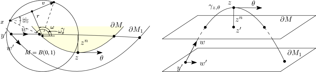
Another way to describe the foliation parameterization, which explains it name, is to think of the hyperplanes $\Sigma_{p}:=\{x^{n}=p\}$, $|p|\ll 1$, as a strictly convex foliation near $q$. Then $\gamma_{z,\theta}$ is the geodesic through $z\in\Sigma_{z^{n}}$ tangent to it with unit direction $\theta\in S_{z}\Sigma_{z^{n}}$. This defines a natural measure on the set of $(z,\theta)$ which we may identify with $\Gamma_{1}$ given by $\mathrm{d}\operatorname{Vol}_{z}\,\mathrm{d}\mu_{\theta}$, where $\mathrm{d}\mu_{\theta}$ is the natural measure on $S_{z}\Sigma_{p}$. Then $(z,\theta)$ belongs locally to the foliation $T\Sigma_{p}$, $|p|\ll 1$ with $p=z^{n}$, $(z^{\prime},\theta)\in T\Sigma_{p}$.

Let us compare the $\partial_{-}SM$ parameterization by $(y^{\prime},w)\in\partial_{-}SM_{1}$ to the $B(\partial M_{1})$ one by $(y^{\prime},w^{\prime})$. As we emphasized above, they are related by a diffeomorphism which becomes singular when $w$ is tangent to $\partial M_{1}$. Such almost tangent geodesics (to $\partial M_{1}$) however do not hit $M$; therefore when parameterizing $If$ with $\operatorname{supp}f\subseteq M$, those two parameterizations are diffeomorphic to each other.

As before, we embed $(M,g)$ in the interior of a simple manifold $(M_{1},g)$ (the metric on $M_{1}$ is an extension of the metric on $M$). We also extend $\kappa$ smoothly to $SM_{1}$ and keep the same notation for the extension. We denote by $I^{M_{1}}_{m,\kappa}$ the geodesic ray transform on $M_{1}$. The set of the oriented geodesics through $M$ will be called $\Gamma$ as before. They are a subset of (the extensions to) all oriented geodesics $\Gamma_{1}$ in $M_{1}$. The latter set is parameterized by $\partial_{-}SM_{1}$; and we identify $\Gamma_{1}$ with it. In particular, $\Gamma_{1}$ becomes a manifold with boundary and $\Gamma$ is a compact submanifold contained in its interior. On $\partial_{-}SM_{1}\cong\Gamma_{1}$ we have two natural measures, as above: one is $\mathrm{d}\Sigma_{1}^{2n-2}$ and the other one is $\mathrm{d}\mu_{1}$, the subscript $1$ indicating that they are on $\Gamma_{1}$. They are equivalent (define equivalent Sobolev spaces) away from $\partial\Gamma_{1}$.

Note that the simplicity is not really needed and assuming non-trapping instead of no conjugate points is enough. The strict convexity of $\partial M$ is convenient for parameterizing $\Gamma$ on $SM_{1}$ but that assumption is not needed either, see e.g., [28].

In the $(z,\theta)$ coordinates, $\Gamma$ is given by $z^{n}\geq 0$. For $u$ supported in $\Gamma$, we define the Sobolev space $H_{\Gamma}^{s}$ as $H^{s}_{\bar{\Omega}}$ above. In particular, when $s$ is a non-negative integer, identifying $\theta$ locally with some parameterization in $\mathbf{R}^{n-1}$, we have locally

This norm is not invariantly defined but under changes of variables, it transforms into equivalent norms. Note that $u$ above is considered as a function defined on $\Gamma_{1}$ but supported in $\Gamma$, as in the definition of $H^{s}_{\bar{\Omega}}$ above.

We make this definition global now. Without changing the notation, let $\Gamma_{1}$ be the manifold of all geodesics with endpoints on $\partial M_{1}$, and let $\Gamma$ be those intersecting $M$. We can choose an open cover of $\Gamma$ consisting of neighborhoods of geodesics tangent to $M$ as above, plus an open set $\Gamma_{0}$ of geodesics passing through interior points only, and having a positive lower bound of the angle they make with $\partial M$. In the latter, we take the classical $H^{s}$ norm w.r.t. the parameterization $(y^{\prime},w)$, for example. In the former neighborhood, we use the norms $H^{s}_{\Gamma}$ defined above. Then using a partition of unity, we extend the norm $H^{s}_{\Gamma}$ to functions defined in $\Gamma_{1}$ and supported in $\Gamma$. This defines a Hilbert space which we call $H^{s}_{\Gamma}$ again.

On the other hand, we have the space $H^{s}_{\Gamma}(\partial_{-}SM_{1})$ of distributions on $\Gamma$ defined through the parameterization of $\Gamma$ given by $(y^{\prime},w)\in\partial_{-}SM_{1}$ in a similar way: we define the $H^{s}$ norm for functions supported in the interior of $\Gamma_{1}$ first (the behavior near the boundary of $\Gamma_{1}$ corresponding to $w$ tangent to $\partial M_{1}$ does not matter in what follows), and then define $H^{s}_{\Gamma}(\partial_{-}SM_{1})$ as the subspace of those $u\in H^{s}(\partial_{-}SM_{1})$ which are supported in $\Gamma$. We define $H^{s}({\Gamma^{\text{\rm int}}})$ similarly, where $\Gamma^{\text{\rm int}}$ is the interior of $\Gamma$.

Proposition 2.1 then implies the following.

We study the mapping properties of $I_{m,\kappa}$, $I_{m,\kappa}^{*}$ restricted a priori to tensor fields/functions supported in fixed compact subsets. This avoids the more delicate question what happens near the boundaries of $M$ and $\Gamma$ but we do not need the latter.

References

- [1] Y. E. Anikonov and V. G. Romanov. On uniqueness of determination of a form of first degree by its integrals along geodesics. J. Inverse Ill-Posed Probl., 5(6):487–490 (1998), 1997.
- [2] I. N. Bernstein and M. L. Gerver. A problem of integral geometry for a family of geodesics and an inverse kinematic seismics problem. Dokl. Akad. Nauk SSSR, 243(2):302–305, 1978.
- [3] J. Boman. An example of nonuniqueness for a generalized Radon transform. J. Anal. Math., 61:395–401, 1993.
- [4] J. Boman. Local non-injectivity for weighted Radon transforms. In Tomography and inverse transport theory, volume 559 of Contemp. Math., pages 39–47. Amer. Math. Soc., Providence, RI, 2011.
- [5] J. Boman and V. Sharafutdinov. Stability estimates in tensor tomography. preprint, 2017.
- [6] N. S. Dairbekov, G. P. Paternain, P. Stefanov, and G. Uhlmann. The boundary rigidity problem in the presence of a magnetic field. Advances in Mathematics, 216(2):535–609, 2007.
- [7] B. Frigyik, P. Stefanov, and G. Uhlmann. The X-ray transform for a generic family of curves and weights. J. Geom. Anal., 18(1):89–108, 2008.
- [8] S. Holman and P. Stefanov. The weighted Doppler transform. Inverse Probl. Imaging, 4(1):111–130, 2010.
- [9] S. Holman and G. Uhlmann. On the microlocal analysis of the geodesic X-ray transform with conjugate points. J. Differential Geom., 108(3):459–494, 2018.
- [10] L. Hörmander. The analysis of linear partial differential operators. II, volume 257. Springer-Verlag, Berlin, 1983. Differential operators with constant coefficients.
- [11] L. Hörmander. The analysis of linear partial differential operators. III, volume 274. Springer-Verlag, Berlin, 1985. Pseudodifferential operators.
- [12] W. McLean. Strongly elliptic systems and boundary integral equations. Cambridge University Press, Cambridge, 2000.
- [13] F. Monard. Numerical implementation of geodesic X-ray transforms and their inversion. SIAM J. Imaging Sci., 7(2):1335–1357, 2014.
- [14] F. Monard, R. Nickl, and G. P. Paternain. Efficient nonparametric Bayesian inference for -ray transforms. Ann. Statist., 47(2):1113–1147, 04 2019.
- [15] F. Monard, P. Stefanov, and G. Uhlmann. The geodesic ray transform on Riemannian surfaces with conjugate points. Comm. Math. Phys., 337(3):1491–1513, 2015.
- [16] R. G. Muhometov. The reconstruction problem of a two-dimensional Riemannian metric, and integral geometry. Dokl. Akad. Nauk SSSR, 232(1):32–35, 1977.
- [17] F. Natterer. The mathematics of computerized tomography. B. G. Teubner, Stuttgart, 1986.
- [18] G. P. Paternain, M. Salo, and G. Uhlmann. Tensor tomography on surfaces. Inventiones Mathematicae, 193(1):229–247, 2013.
- [19] L. Pestov and G. Uhlmann. On characterization of the range and inversion formulas for the geodesic X-ray transform. Int. Math. Res. Not., (80):4331–4347, 2004.
- [20] M. Salo and G. Uhlmann. The attenuated ray transform on simple surfaces. J. Differential Geom., 88(1):161–187, 2011.
- [21] V. A. Sharafutdinov. Integral geometry of tensor fields. Inverse and Ill-posed Problems Series. VSP, Utrecht, 1994.
- [22] V. A. Sharafutdinov. A finiteness theorem for the ray transform on a Riemannian manifold. Dokl. Akad. Nauk, 355(2):167–169, 1997.
- [23] V. A. Sharafutdinov. Ray transform on Riemannian manifolds, lecture notes, UW–Seattle. available at: http://www.ima.umn.edu/talks/workshops/7-16-27.2001/sharafutdinov/, 1999.
- [24] P. Stefanov. A sharp stability estimate in tensor tomography. Journal of Physics: Conference Series, 124(1):012007, 2008.
- [25] P. Stefanov. Semiclassical sampling and discretization of certain linear inverse problems. arXiv:1811.01240, 2019.
- [26] P. Stefanov and G. Uhlmann. Stability estimates for the X-ray transform of tensor fields and boundary rigidity. Duke Math. J., 123(3):445–467, 2004.
- [27] P. Stefanov and G. Uhlmann. Boundary rigidity and stability for generic simple metrics. J. Amer. Math. Soc., 18(4):975–1003, 2005.
- [28] P. Stefanov and G. Uhlmann. Integral geometry on tensor fields on a class of non-simple Riemannian manifolds. Amer. J. Math., 130(1):239–268, 2008.
- [29] P. Stefanov and G. Uhlmann. An inverse source problem in optical molecular imaging. Anal. PDE, 1(1):115–126, 2008.
- [30] P. Stefanov and G. Uhlmann. Local lens rigidity with incomplete data for a class of non-simple Riemannian manifolds. J. Differential Geom., 82(2):383–409, 2009.
- [31] P. Stefanov and G. Uhlmann. The geodesic X-ray transform with fold caustics. Anal. PDE, 5(2):219–260, 2012.
- [32] P. Stefanov, G. Uhlmann, and A. Vasy. Local and global boundary rigidity and the geodesic X-ray transform in the normal gauge. arXiv:1702.03638, 2017.
- [33] P. Stefanov, G. Uhlmann, and A. Vasy. Inverting the local geodesic X-ray transform on tensors. Journal d’Analyse Mathématique, 136(1):151–208, 2018.
- [34] G. Uhlmann and A. Vasy. The inverse problem for the local geodesic ray transform. Invent. Math., 205(1):83–120, 2016.