SI-HEP-2015-26
QFET-2015-33
Phenomenological Implications of an
SUSY GUT of Flavour
Abstract
We discuss the characteristic low energy phenomenological implications of an Supersymmetric Grand Unified Theory (SUSY GUT) whose flavour structure is controlled by the family symmetry , which provides a good description of all quark and lepton masses, mixings as well as CP violation. Although the model closely mimics Minimal Flavour Violation (MFV) as shown in [1], here we focus on the differences. We first present numerical estimates of the low energy mass insertion parameters, including canonical normalisation and renormalisation group running, for well-defined ranges of SUSY parameters and compare the naive model expectations to the numerical scans and the experimental bounds. Our results are then used to estimate the model-specific predictions for Electric Dipole Moments (EDMs), Lepton Flavour Violation (LFV), and meson mixing as well as rare decays. The largest observable deviations from MFV come from the LFV process and the electron EDM.
1 Introduction
The flavour problem has been around for a long time, but only relatively recently has new information been provided in the form of neutrino mass and lepton mixing. Subsequently, a lot of effort has been put into trying to formulate a theory of flavour (for reviews see e.g. [2]) which can account for the observed pattern of fermion masses and mixing, while providing more accurate predictions for the less well measured (or unmeasured) flavour parameters in the neutrino sector, see e.g. [3].
A possible additional source of experimental information which could shed light on the flavour puzzle would be the observation of rare flavour changing processes at rates beyond that predicted by the Standard Model (SM). Such observations could in principle provide insight into the nature of the theory of flavour beyond the SM. So far, experiment has unfortunately not measured any flavour or CP violation beyond SM expectations. Indeed all data are consistent with the concept of Minimal Flavour Violation (MFV) [4], in which all flavour and CP-violating transitions are governed by the CKM matrix and the only relevant local operators are the ones that are relevant in the SM. Although the formulation of MFV in an effective field theory, involving an approximate symmetry444In the framework of Grand Unified Theories (GUTs) it is not possible to implement symmetry at the GUT scale. However, in GUTs based on [5] or Pati-Salam [6], it is certainly possible to introduce an flavour symmetry, and this has been shown to be sufficient [7]. broken by the Yukawa matrices, allows some new operators which can in principle give significant contributions [8, 9], in all cases, MFV predicts very SM-like flavour and CP violation consistent with observation.
The absence of flavour violation is consistent with the absence of any new physics beyond the SM, such as Supersymmetry (SUSY) which, if softly broken at the TeV scale, would in general imply large deviations from SM flavour and CP violation [10]. For example, SUSY models involve one-loop diagrams that induce Flavour Changing Neutral Current (FCNC) processes such as and at rates which are proportional to the mass insertion parameters, i.e. the off-diagonal elements of the scalar mass matrices in the super-CKM (SCKM) basis where the Yukawa matrices are diagonal [10, 11]. Such SUSY contributions are very small in the the Constrained Minimal Supersymmetric Standard Model (CMSSM) where the squark and slepton mass squared matrices are proportional to the unit matrix at the high energy scale and the trilinear -terms are aligned with the Yukawa matrices, resulting in an (approximate) MFV-like structure at low energy [10]. But there is no convincing theoretical basis for either the CMSSM or MFV. Moreover, in SUSY GUTs, the CMSSM framework while providing suppressed flavour violation, cannot easily control CP violation in the form of Electric Dipole Moments (EDMs) which remains a challenge [10]. However, the real challenge is to justify the assumptions of MFV or the CMSSM, while at the same time providing a realistic explanation of quark and lepton (including neutrino) masses, mixing and CP violation.
Following the discovery of neutrino mass and mixing, there has been an impetus to revisit the favour problem using a family symmetry of some kind, in particular discrete non-Abelian family symmetry [2]. It was realised that in such models, spontaneous CP and flavour violation could solve the CP and flavour problems of the SM [12, 13] without any ad hoc assumptions about MFV or the CMSSM. The family symmetry that is responsible for the structure of the Yukawa sector will automatically control the soft SUSY breaking sector as long as the SUSY breaking hidden sector respects the family symmetry. This is realised for instance in supergravity induced SUSY breaking.
Considering a SUSY framework, the choice of an family symmetry [13, 14] provides a benchmark scenario where flavour and CP violation is controlled by family symmetry. The spontaneous breaking of family and CP symmetry by Vacuum Expectation Values (VEVs) of the so-called flavon fields perturbs the SUSY breaking sector, thereby generating distinct deviations from MFV or the CMSSM. Unfortunately, these signatures which were expected to appear in Run 1 of the LHC [15] did not in fact materialise, and the allowed parameter space has been much reduced [16]. At leading order, the CMSSM is enforced by the family symmetry acting on the squark and slepton mass squared matrices. When is broken by flavon VEVs, to generate quark and lepton flavour, those flavons appearing in the Kähler potential give important contributions to the kinetic terms, requiring extra canonical normalisation [17]. Since SUSY breaking also originates from the Kähler potential, the flavons also modify the couplings of squarks and sleptons to the fields with SUSY breaking -terms, where the corrections have a different form to the flavon corrections appearing in the superpotential. All of this occurs at the high scale. Additional flavour violation is generated by renormalisation group (RG) running down to low energy, taking into account the seesaw mechanism [18] and threshold corrections [19].
In this paper we discuss the characteristic low energy phenomenological implications of an Supersymmetric Grand Unified Theory (SUSY GUT) whose flavour structure is controlled by the family symmetry , which provides a good description of all quark and lepton masses, mixings as well as CP violation. In a recent paper we showed how MFV emerges approximately in this setup [1]. Assuming a SUSY breaking mechanism which respects the family symmetry, we calculated in full explicit detail the low energy mass insertion parameters in the SCKM basis, including the effects of canonical normalisation and renormalisation group running, showing that the peculiar flavour structure of the model, defined by the small family symmetry , is sufficient to approximately mimic MFV.555Depending on the implementation of a particular family symmetry, SUSY GUTs of flavour typically realise some approximation of MFV at high as well as low scales [20]. However there are important phenomenological differences which can provide tell-tale signatures of the model, and it is the main purpose of this paper to discuss these in detail. In other words, we exploit the low energy mass insertion parameters of the model calculated in [1] to analyse a panoply of rare and flavour changing processes as well as EDMs in both the lepton and quark sectors. The results are quite illuminating: while we find only small new effects in physics, very large effects arise for Lepton Flavour Violation (LFV) and the electron EDM which are therefore predicted to be observed soon.
The layout of the remainder of the paper is as follows. In Section 2 we give a succinct summary of the analytic Yukawa matrices and mass insertion parameters calculated in [1]. In Section 3 we discuss numerical estimates of the low energy mass insertion parameters for ranges of SUSY parameters which are consistent with the bounds from direct searches for squarks and sleptons at LHC Run 1. We compare the naive model expectations to the numerical scans and the experimental bounds. In Section 4 these results are then used to estimate the predictions for EDMs, LFV, and meson mixing as well as rare decays. The largest observable deviations from MFV come from the LFV process and the electron EDM. Section 5 concludes the paper.
2 Yukawa matrices and SUSY breaking parameters
In this section, we briefly summarise the GUT scale Yukawa matrices and soft SUSY breaking parameters constructed within the framework of the family symmetry model in [1]. Working in a power expansion of the Wolfenstein parameter [21], we present all expressions to Leading Order (LO). The entries of the flavour matrices are generally complex, where the phases are given in terms of two free parameters , , with the exception of the soft trilinear terms whose phases are not identified with the corresponding Yukawa phases but are kept as free parameters, even though their flavour structure is the same as that of the Yukawas. Details on this aspect can be found in [1]. In the present work, we will comment on the consequences of this generalisation where relevant.
2.1 Yukawa sector
The fermion structure was already scrutinised in [22], and we have completed this analysis by including the effects of canonical normalisation. In the basis with canonical kinetic terms, that is after redefining the superfields such that the Kähler metrics are identified with the unit matrix, the Yukawa matrix for the up-type quarks reads
| (2.4) |
where and are real order one coefficients, with the former stemming from the Yukawa part of the superpotential of the theory and the latter from the Kähler potential. In particular, and appear in the non-canonical Kähler metric of the -plets, in the (12), (23) and (13) elements, respectively.
The Yukawa matrices for the down-type quarks and charged leptons take the form
| (2.8) | |||||
| (2.12) |
Again, these expressions are given in the canonical basis and all coefficients are real and of order one. , and arise from the superpotential operators and from the Kähler potential, where it enters symmetrically in all off-diagonal elements of the non-canonical Kähler metric of the -plets.
Finally, the Dirac neutrino Yukawa matrix in the canonical basis is given by
| (2.16) |
which is real up to LO in . The parameters and originate from the superpotential, while is associated to the Kähler metric of the right-handed neutrinos. Note that this metric is identical to that of the -plets, up to renaming the order one coefficients, see [1] for details.
Transforming the left- and right-handed superfields by unitary matrices , we obtain the canonically normalised diagonal and positive Yukawas in the SCKM basis
| (2.17) |
| (2.18) |
Up to phase convention, the CKM matrix is given by , leading to the mixing angles
| (2.19) |
The mixing arises purely from the down-type quark sector and incorporates the
Gatto-Sartori-Tonin relation [23]
. The amount of CP violation is given by
the Jarlskog invariant [24]
| (2.20) |
These results are in agreement with the LO expressions derived in [22], where canonical normalisation effects were ignored. As discussed in [1], the LO results for the quark and charged lepton masses and mixing angles remain unaffected by the process of canonicalising the kinetic terms. We point out that these 13 observables of the charged fermion sector are given in terms of only 8 input parameters (, , , and ) at LO.
2.2 Soft SUSY breaking sector
The soft trilinear -terms and the Yukawa couplings originate in the same superpotential terms. Hence, they have a similar flavour structure and, in the basis of canonical kinetic terms, the soft flavour matrices , where denotes the scale of the trilinear terms, can be deduced from Eqs. (2.4-2.16) by simply replacing , , , , , , and . Here, the Yukawa phases are all given in terms of as follows: , and . On the other hand, the trilinear phases are kept free.
Turning to the soft scalar mass squared matrices in the canonical basis, we find
| (2.24) |
for the -plets as well as
| (2.28) |
for the -plets and the right-handed neutrinos, with the latter being associated to the coefficients with index . For convenience, we absorb the universal order one parameter on the diagonal into the soft SUSY breaking mass , so that the leading contribution to the diagonal entries of is one.
2.3 Mass insertion parameters
In order to study the phenomenological implications of the soft SUSY breaking sector, it is useful to rotate all quantities into the physical basis where the Yukawa matrices are diagonal and positive, i.e. the SCKM basis. Any misalignment between the fermion and sfermion flavour matrices constitutes a source of flavour violation, with the off-diagonal entries of the sfermionic mass matrices contributing to FCNCs. The sfermion mass matrices are given as
| (2.29) |
where and denote the soft flavour matrices in the SCKM basis, and are the diagonal Yukawa matrices. is the (real) higgsino mass parameter, and the VEVs of the two neutral Higgses are defined as
| (2.30) |
where and GeV. The indices and refer to the chirality of the corresponding SM fermions and . With these definitions, the amount of flavour violation can be measured in terms of the dimensionless mass insertion parameters [11]
| (2.31) |
where the average masses in the denominators are defined by
| (2.32) |
We mention in passing that the phase structure of the mass insertion parameters depends on the choice of the phase conventions of the CKM and PMNS matrices. In [1], we have worked out the expressions in Eq. (2.31) explicitly for our model at the GUT scale, choosing a phase convention in which and take their standard form.
The effects of RG running down to the low energy scales where experiments are performed were also estimated, using the leading logarithmic approximation. Introducing the parameters
| (2.33) |
we performed a two-stage running () from to , where the right-handed neutrinos are integrated out, and () from to . For GeV, GeV and GeV, is of the order of our expansion parameter and . In terms of their -suppression, the resulting flavour structures of the low energy mass insertion parameters read
| (2.43) | |||
| (2.53) | |||
| (2.63) |
Appendix A provides the explicit expressions for each entry in terms of the parameters of the model.
3 Numerical analysis
3.1 Parameter range
Numerical results for the running quark and charged lepton masses as well as for the quark mixing angles at the GUT scale can be found in [25]. The matching conditions from the SM to the Minimal Supersymmetric Standard Model (MSSM), imposed at the SUSY scale, take the form
| (3.1) |
for the singular values of the Yukawa matrices. Similarly, we have for the CKM mixing
| (3.2) |
Here
| (3.3) |
represent SUSY radiative threshold corrections that are parametrised by , with explicit expressions for available in [26]. The unprimed parameters correspond to corrections to the first two generations, the primed ones to the third generation, and the one with index “” to a correction due to the soft SUSY breaking trilinear terms. The parameter follows from the absorption of into ,
| (3.4) |
with the approximation being valid for . In the limit where threshold effects for the charged leptons are neglected, simply reduces to .
Our model predicts , where the hat indicates the diagonalised Yukawa sector at the GUT scale. As a consequence, very large values of are excluded, and we only study the parameter space in which , keeping the value of below four. In order to obtain viable ranges for our Yukawa input parameters, we plot , and against using the results for the diagonalised Yukawa sector at the GUT scale provided in [25]. We remark that , and are extracted from the lepton sector. We fit the resulting curves using the relative uncertainties , , , , see [25]. Concerning and , we take and , allowing for higher order corrections to the mass ratios that would reduce the discrepancy between the values of predicted from the lepton and the quark sectors and maximise the GUT scale value of . Due to the implementation of the Georgi-Jarlskog relation [27], it is equal to 9 in our model at LO, while its preferred range is [25], which is independent of threshold corrections and also not sensitive to a change of the SUSY scale.
We estimate the low energy Yukawa couplings using the leading logarithmic approximation as described in [1]. Clearly, the resulting low energy Yukawa matrices are only valid up to that approximation. Mindful of such limitations, we obtain
| (3.5) | |||||
| (3.6) | |||||
| (3.7) |
where the corrections from the RG running are encoded in the parameters
| (3.8) | |||||
| (3.9) |
Here, denotes the universal gauge coupling constant at the GUT scale. Our scan produces the following values for the right-hand sides of Eq. (3.1)
| (3.10) |
which have to be compared to the SM values, taken from Table 2 of [25],
| (3.11) | |||||
The corresponding ranges of the order one input parameters of the Yukawa sector are listed in the first five rows of the first column of Table 1. All other coefficients that are not fixed by this fit, are scanned over the interval , with the following exceptions: we allow the absolute value of the Dirac neutrino Yukawa coupling to be as small as but not larger than , such that it does not exceed the maximum allowed value of . We also relax the lower bounds on , and and extend the upper bound on , such that they are allowed to get the same values as the corresponding Yukawa coefficients. The coefficients and of the soft Higgs mass squares,
| (3.12) |
are taken to be positive, just like the coefficients , and of the leading order diagonal elements of the soft scalar mass squared matrices. Phases are generally allowed to take arbitrary values within . As mentioned earlier, is varied between 5 and 25. Concerning the CMSSM parameters, we define
| (3.13) |
and scan over TeV, TeV as well as in order to avoid charge and colour breaking minima.666In our numerical scan, we have checked that the potentials are always bounded from below and that the corresponding minima do not break charge or colour [28].
| Yukawa terms | Range | Soft trilinear terms | Range |
|---|---|---|---|
| Kähler metric | Range | Soft mass terms | Range |
| SUSY masses | Range | SUSY ratios | Range |
| TeV | |||
| TeV | |||
The parameter, which we take as real, is given at the electroweak scale by the relation777The lack of any evidence for low energy supersymmetry requires a certain amount of cancellation between the terms of Eq. (3.14), see e.g. [29].
| (3.14) |
where denotes the boson mass [30]. and are radiative corrections, with the most important contributions coming from the stops
| (3.15) | |||||
| (3.16) |
In these expressions, , and denote the low energy Yukawa and trilinear couplings and the low energy parameter, respectively. Moreover
| (3.17) |
with denoting the Weinberg angle. , and are the low energy (33) elements of the squark mass matrices defined in Eq. (2.29). The so-determined parameter can then be used to calculate the physical Higgs mass. Adopting the approximate formulas of Section 2.4 of [31], we demand that the resulting Higgs mass lies within the interval GeV. Additionally, we impose cuts on the SUSY parameters from direct searches by requiring that the first and the second generation squark masses are larger than TeV.
3.2 Estimates of the low energy mass insertion parameters
In this section, we analyse the predictions for the low energy mass insertion parameters whose explicit expressions are given in Appendix A. Tables 2-6 provide naive expectations for the individual s, where we take into account the -suppression and the main effects of the RG running, while setting any order one coefficients to one. Clearly, we still expect to see a spread within a few orders of magnitude due to the variation of the SUSY scale and the order one coefficients. The third columns of Tables 2-6 list existing experimental bounds. The full ranges of our s arising from scanning over the input parameters, given in Table 1, are depicted in Figures 1-3.
3.2.1 Up-type quark sector
| Parameter | Naive expectation | Exp. bound |
|---|---|---|
|
[32]
|
||
| [32] | ||
| [33] | ||
| [34] | ||
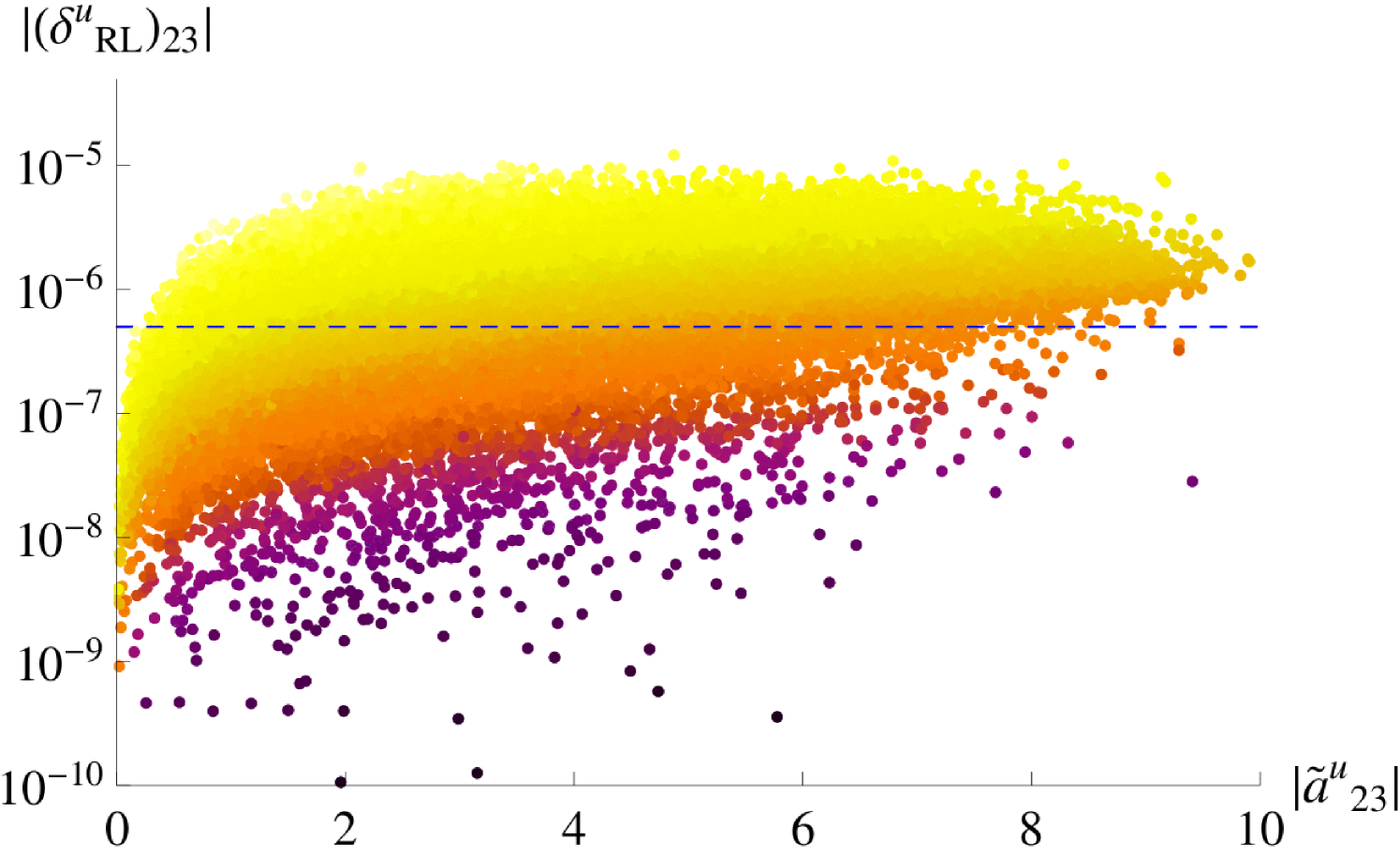
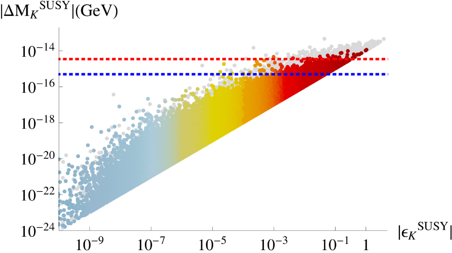
The strongest constraints on the up-type mass insertion parameters involve the (12) sector and stem from mixing. The SM contribution to this amplitude conserves CP to a good approximation and provides significant constraints on the imaginary parts of , . These limits were derived in [32], assuming equal squark and gluino masses of 1 TeV. We quote them in the third column of Table 2, rescaled to masses of 1.5 TeV. The limits on the and parameters are identical to the and ones due to the symmetric form of the gluino-squark box diagram. The index refers to the assumption that , as is the case in our model. In the second column of Table 2, we give a naive estimate for . For , as suggested from maximising the Jarlskog invariant of Eq. (2.20), these quantities vanish to LO. Since is at most , we only show the full range of the absolute value of that parameter in Figure 1, plotted against the corresponding GUT scale coefficient , defined in Eq. (A.1). This coefficient quantifies the mismatch between the Kähler metric and the soft mass matrix elements for the -plets and can be as large as 6 when the associated parameters contribute constructively and receive their maximum values in the scan. The effects of the RG running are trivial and depend only on ; for and , we estimate a value of around , shown by the blue dashed line in Figure 1. With increasing , we obtain even smaller values, as the RG suppression is increased. The red dotted line shows the experimental limit, adapted from [32] and valid for .
The and parameters of the sector () have GUT scale coefficients with the same range as the parameters of the (12) sector but a different RG suppression due to the milder running of the third generation sfermionic masses. This is represented by the factor appearing in Eq. (A.13), where and are defined in Eqs. (2.33,A.7), respectively. Approximating these s as shown in Table 2 and taking , as well as , we expect and to vary around and , respectively. The existing bounds on these variables from flavour changing effects are very weak, leaving them essentially unconstrained. mixing can place a bound on of the order of at most, as described in [33].
![[Uncaptioned image]](https://cdn.awesomepapers.org/papers/c80652bf-5bca-4d5e-a453-07e951629fda/x1.png)
![[Uncaptioned image]](https://cdn.awesomepapers.org/papers/c80652bf-5bca-4d5e-a453-07e951629fda/x2.png)
![[Uncaptioned image]](https://cdn.awesomepapers.org/papers/c80652bf-5bca-4d5e-a453-07e951629fda/x3.png)
![[Uncaptioned image]](https://cdn.awesomepapers.org/papers/c80652bf-5bca-4d5e-a453-07e951629fda/x4.png)
![[Uncaptioned image]](https://cdn.awesomepapers.org/papers/c80652bf-5bca-4d5e-a453-07e951629fda/x5.png)
![[Uncaptioned image]](https://cdn.awesomepapers.org/papers/c80652bf-5bca-4d5e-a453-07e951629fda/x6.png)
![[Uncaptioned image]](https://cdn.awesomepapers.org/papers/c80652bf-5bca-4d5e-a453-07e951629fda/x7.png)
![[Uncaptioned image]](https://cdn.awesomepapers.org/papers/c80652bf-5bca-4d5e-a453-07e951629fda/x8.png)
The parameters of type have a slightly different behaviour. They are proportional to the factor which, for TeV, can cause an extra suppression of up to . Because of this factor, the parameters show a dependence on the mass scale, even at the GUT scale. are also generally proportional to the mismatch of the ratios of soft trilinear over Yukawa sector coefficients for the -th and the -th generation and vanish, barring RG induced corrections, if those are aligned. To estimate the magnitude of these parameters in Table 2, we take , , and , while their full ranges are shown in Figure 1. The parameter was zero at the GUT scale but receives a contribution through the RG running of the order of . Similarly, , which was suppressed by at the GUT scale, receives a similar running contribution which comes in at an even lower order, namely . Such an effect is not found in any other parameter. Finally, we remark that as well as are zero up to order , where we truncate our expansion.
The limits on the parameters of the sector ( originate mainly from the requirement that the potential be bounded from below with a vacuum that does not break charge or colour [28]. We have already constrained the trilinear parameters accordingly and do not comment on those effects any further. Other bounds on the off-diagonal parameters can be deduced by demanding that the supersymmetric radiative corrections to the CKM matrix elements do not exceed their experimental values [35]. The limit for quoted in Table 2 has been obtained in [34] by considering chargino loop contributions to . In our model, all up-type mass insertion parameters of the type turn out to be safely below any current bound.
3.2.2 Down-type quark sector
| Parameter | Naive expectation | Exp. bound |
|---|---|---|
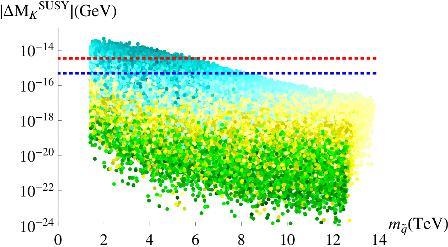
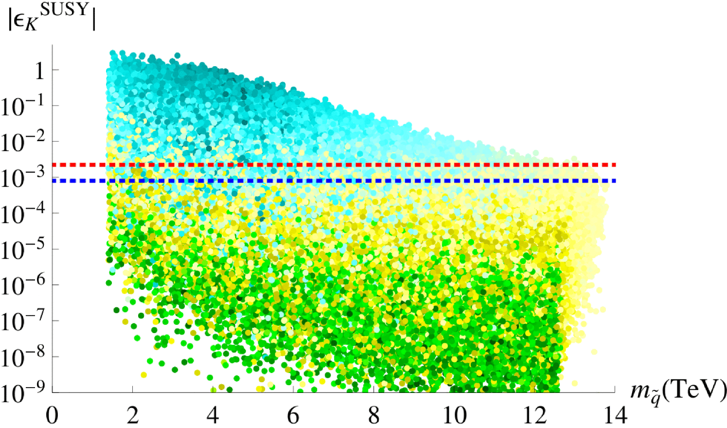
We first consider the (12) elements of the down-type mass insertion parameters , where . The corresponding bounds are derived from the results of [36] which we have rescaled to TeV and . These bounds are summarised in the third column of Table 3 and have been extracted using observables related to Kaon mixing. They are given separately for the real and imaginary parts due to a relative difference of an order of magnitude.
In our model, is real at LO, while the next-to-leading order (NLO) contribution is a linear combination of and . Therefore, is proportional to . Setting , i.e. the value preferred by the Jarlskog invariant , we expect to take its maximum value. In Figure 2 we only plot the absolute value of this mass insertion parameter versus its GUT scale coefficient , see Eq. (A.1), which can take values between zero and twelve. Our naive numerical estimate of , approximated as shown in the second column of Table 3, is of the order of for , visualised by the blue dashed line in Figure 2. Since the experimental limits are given as ranges, we depict them by the red shaded region.
![[Uncaptioned image]](https://cdn.awesomepapers.org/papers/c80652bf-5bca-4d5e-a453-07e951629fda/x11.png)
![[Uncaptioned image]](https://cdn.awesomepapers.org/papers/c80652bf-5bca-4d5e-a453-07e951629fda/x12.png)
![[Uncaptioned image]](https://cdn.awesomepapers.org/papers/c80652bf-5bca-4d5e-a453-07e951629fda/x13.png)
![[Uncaptioned image]](https://cdn.awesomepapers.org/papers/c80652bf-5bca-4d5e-a453-07e951629fda/x14.png)
![[Uncaptioned image]](https://cdn.awesomepapers.org/papers/c80652bf-5bca-4d5e-a453-07e951629fda/x15.png)
![[Uncaptioned image]](https://cdn.awesomepapers.org/papers/c80652bf-5bca-4d5e-a453-07e951629fda/x16.png)
![[Uncaptioned image]](https://cdn.awesomepapers.org/papers/c80652bf-5bca-4d5e-a453-07e951629fda/x17.png)
![[Uncaptioned image]](https://cdn.awesomepapers.org/papers/c80652bf-5bca-4d5e-a453-07e951629fda/x18.png)

The parameter is proportional to , so that vanishes for , while the corresponding real part is maximised. The RG suppression is again trivial, only depending on , while the GUT scale parameter is proportional to , see Eq. (A.1). When and , the absolute value of the mass insertion reaches its maximum of , as can be seen in the associated plot in Figure 2. On the other hand, for , and , it can scale down to about . Note that , as can be seen in Eqs. (A.32,A.33).
The mass insertion parameters receive an extra suppression from the factor , for which we use the value of in our naive numerical estimates. Then, for , we expect these parameters to vary around , see the last two rows of Table 3. As can be seen in Figure 2, our model predictions lie well below the limits. Furthermore, if the Yukawa and soft trilinear phase structures are aligned, the phases within cancel and becomes real at the given order in .
As parts of our parameter space place the down-type mass insertion parameter within a region possibly excluded by Kaon mixing observables, we study the relevant contributions in Section 4 in more detail. Due to additional strong constraints on the product of and mass insertion parameters, we see that actually a large fraction of the parameter space is excluded.
| Parameter | Naive expectation | Exp. bound |
|---|---|---|
The bounds on , are related to transitions. They are taken from [37] and were derived by demanding that the contribution of each individual mass insertion parameter to the flavour observables , and does not exceed the current experimental limits. The analysis was performed for six representative points of the MSSM parameter space which are compatible with LHC SUSY and Higgs searches as well as an explanation of the discrepancy of from its SM value in terms of one-loop SUSY contributions from charginos and neutralinos. We present the extracted bounds in the third column of Table 4, where the intervals arise due to the dependence on the SUSY spectra. We note that, for simplicity, all s were assumed to be real in [37].
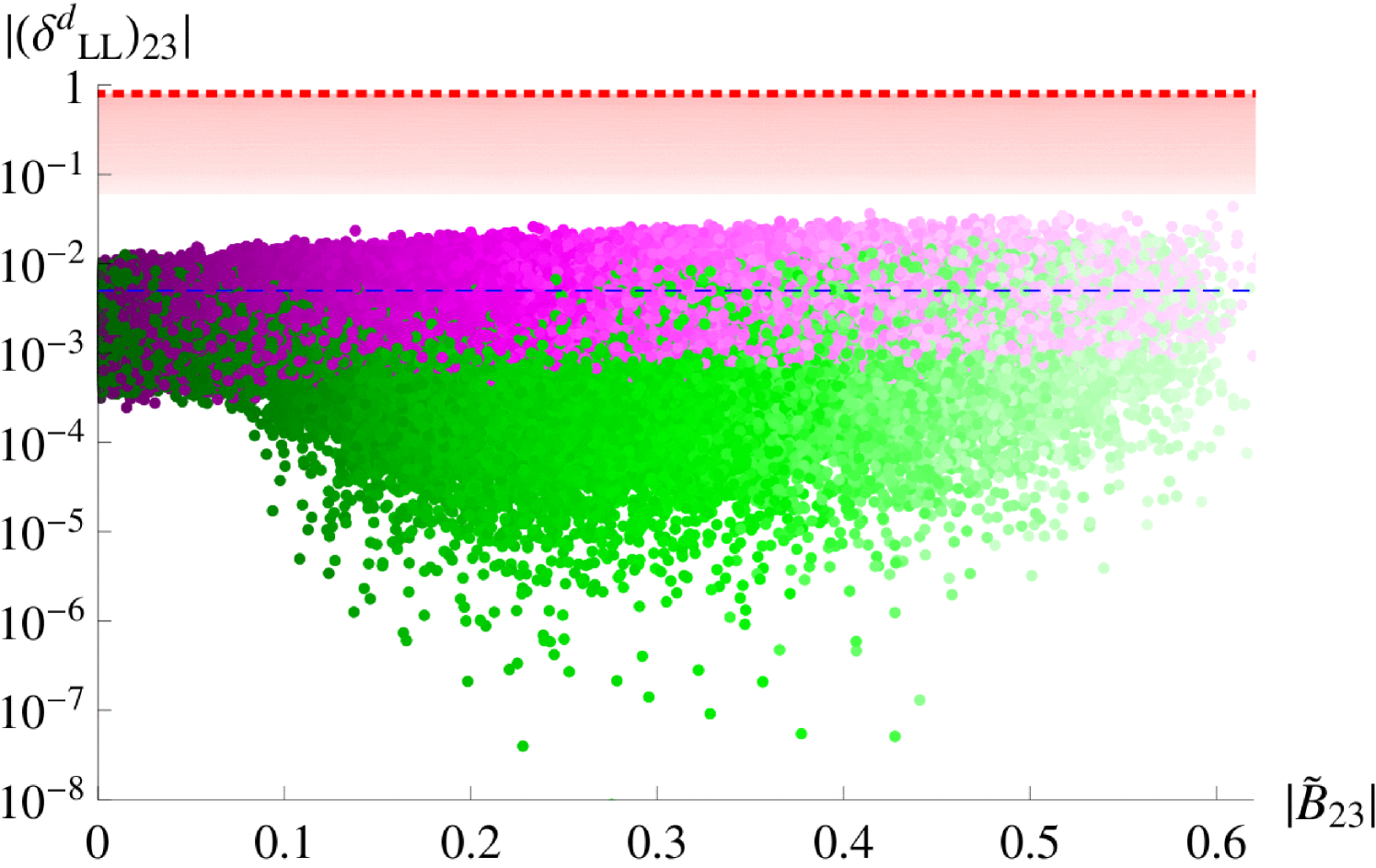
At the GUT scale, the parameter is proportional to ; it can therefore vanish at that order if . In that case, it would still receive a non-zero contribution through the running, as can be seen in Eq. (A.31), through the factor , defined in Eq. (A.7). To see this effect, we expand to first order in the running parameter , defined in Eq. (2.33), taking the limit . Then, for , and , we expect the absolute value of to vary around for , as shown by the blue dashed line in Figure 2. The spread towards smaller values of as deviates from zero, is mainly due to the parameter space where is negative, thereby partly cancelling the contribution. As can be seen in Figure 2, all generated points lie below the limits of the corresponding (23) sector.
| Parameter | Naive expectation | Exp. bound |
|---|---|---|
The experimental bounds for are taken from [36], where they were extracted from mixing related observables and given in terms of and . Their orders of magnitude are at most of the same order as , and for TeV and they are summarised in the third column of Table 5. The limits for the and type s are equal to the and type ones, respectively, as the gluino contribution to the box diagram for meson mixing is symmetric under .
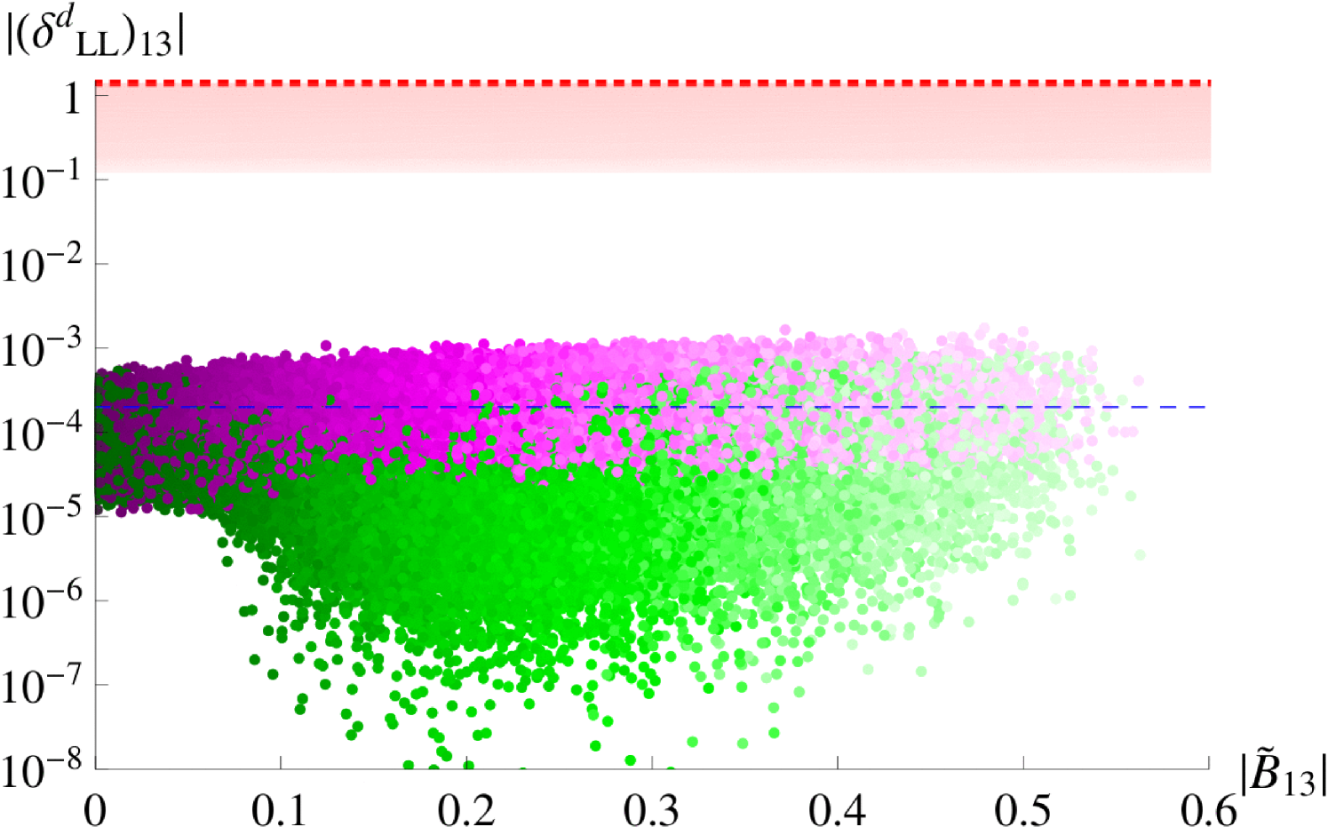
In our model, we expect to have a similar behaviour as but with an extra suppression of . Furthermore, mimics with an extra enhancement factor of . The parameters (13) and (23) sectors are of the same order in and should therefore have a similar numerical range. All (13) sector mass insertion parameters lie below the limits set by mixing, as can be seen in Figure 2.
3.2.3 Charged lepton sector
| Parameter | Naive expectation | Exp. bound |
|---|---|---|
The bounds on the mass insertion parameters , , of the charged lepton sector are taken from [38]. They were derived by studying radiative, leptonic and semileptonic LFV decays as well as conversion in heavy nuclei. The analysis was performed for six representative points in the MSSM parameter space, which are in agreement with LHC SUSY and Higgs searches as well as data on . Moreover, four additional, more general two-dimensional scenarios, characterised by universal squark and slepton mass scales, were considered in [38]. The derived limits vary within an order of magnitude in all cases and are summarised in the third column of Table 6. We note that all s were assumed to be real in [38] for simplicity.
At the GUT scale, the mass insertion parameter is proportional to . Its absolute value is equal to due to the framework. However, the parameter of the lepton sector, given in Eq. (A.41), receives large RG corrections which encode seesaw effects. At the low energy scale, it is non-zero even for , due to the term proportional to the small parameter which is defined in Eq. (2.33) and originates from the running between the GUT scale and the scale of the right-handed neutrinos. In the second column of Table 6, we estimate this effect by considering . We then expand to first order in and consider , where and are defined in Eqs. (A.8,A.9). For , and , we expect the low energy to vary around . However, the non-trivial expression of , cf. Eqs. (A.41,A.54), creates a spread of about two orders of magnitude around this value. As increases, the mass insertion parameter lies above the limits given in Table 6. As can be seen from Figure 3, the non-observation of places stronger constraints on the down-type quark s than the direct bounds from the quark sector. Analogous to the down-type parameters, the absolute values of the (12), (23) and (13) lepton parameters are identical, see Eqs. (A.41,A.42).
![[Uncaptioned image]](https://cdn.awesomepapers.org/papers/c80652bf-5bca-4d5e-a453-07e951629fda/x22.png)
![[Uncaptioned image]](https://cdn.awesomepapers.org/papers/c80652bf-5bca-4d5e-a453-07e951629fda/x23.png)
![[Uncaptioned image]](https://cdn.awesomepapers.org/papers/c80652bf-5bca-4d5e-a453-07e951629fda/x24.png)
![[Uncaptioned image]](https://cdn.awesomepapers.org/papers/c80652bf-5bca-4d5e-a453-07e951629fda/x25.png)
![[Uncaptioned image]](https://cdn.awesomepapers.org/papers/c80652bf-5bca-4d5e-a453-07e951629fda/x26.png)
![[Uncaptioned image]](https://cdn.awesomepapers.org/papers/c80652bf-5bca-4d5e-a453-07e951629fda/x27.png)
![[Uncaptioned image]](https://cdn.awesomepapers.org/papers/c80652bf-5bca-4d5e-a453-07e951629fda/x28.png)
![[Uncaptioned image]](https://cdn.awesomepapers.org/papers/c80652bf-5bca-4d5e-a453-07e951629fda/x29.png)
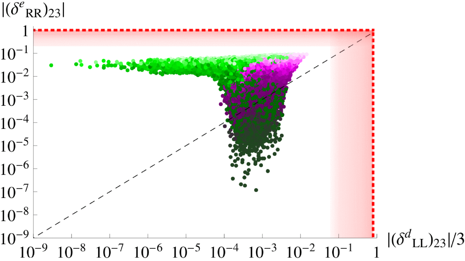
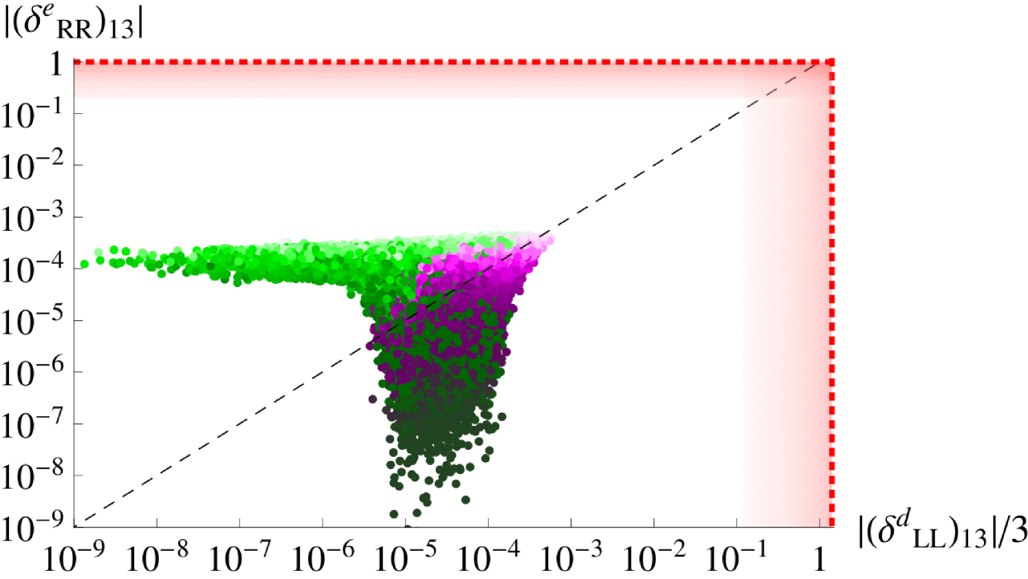
Similarly, at the GUT scale, the absolute values of the parameters in the lepton sector are equal to the ones of the down-type sector times the Georgi-Jarlskog factor of . For the (12) s, the RG running effects are trivial, consisting only of a suppression through , which is milder in the lepton sector where the numerical prefactor of is , as compared to a factor of in the quark one. For the (13) and (23) parameters, the non-trivial running effects in the quark sector are obvious in Figure 3, where we see that even though can get very small for negative , can only receive such small values when , see e.g. Eqs. (A.30,A.44).
Finally, the variation of the parameters can be understood in an analogous way to the one described in the quark sector. , with the exception of the (23) parameters which are not equal due to a term which involves a , thereby receiving an extra factor of 9 for the leptons, see Eqs. (A.40,A.52) together with Eq. (A.2). As in the down-type sector, and we only show the (12) parameter in Figure 3 which features the strongest experimental constraint.
4 Phenomenological implications
In the preceding section, we found that parts of the parameter space spanned by the (12) mass insertion parameters of the down-type and charged lepton sector are excluded due to experimental limits set by and Kaon mixing observables. The corresponding bounds are available in the literature and their derivation is highly dependent on the assumed SUSY mass spectra. Possible interference effects between contributions from multiple parameters to a given observable can additionally have significant effects. These are usually ignored when setting “model independent” limits on mass insertion parameters.
In this section, we therefore investigate the phenomenological implications of the deviations of our model from MFV. In particular, we focus on the predictions for and . We also scrutinise whether the phase structure of our model can survive the strong limits set by electric dipole moments. Since the analysis in [37], which provides the limits on , assumes real parameters throughout, we also study how our model contributes to the time-dependent CP asymmetry associated with the decay . For completeness, we check that the limits set by the decay and the mass differences are satisfied. Finally, we also consider the branching ratios of and
Adopting the leading logarithmic approximation, the low energy gaugino masses [39]
| (4.1) |
with , and , are given by
| (4.2) |
4.1 Electron EDM
The current experimental limit for the electric dipole moment of the electron stems from the ACME collaboration [40] and is given by
| (4.3) |
This tiny value poses a strong constraint on the phases of any model. The supersymmetric contributions depend on the mass insertion parameters as follows [41]888The corresponding expression in [15] also includes triple mass insertions of type and . In our model, these give suppressed contributions to of order and , respectively, which can be safely neglected.
| (4.4) | |||||
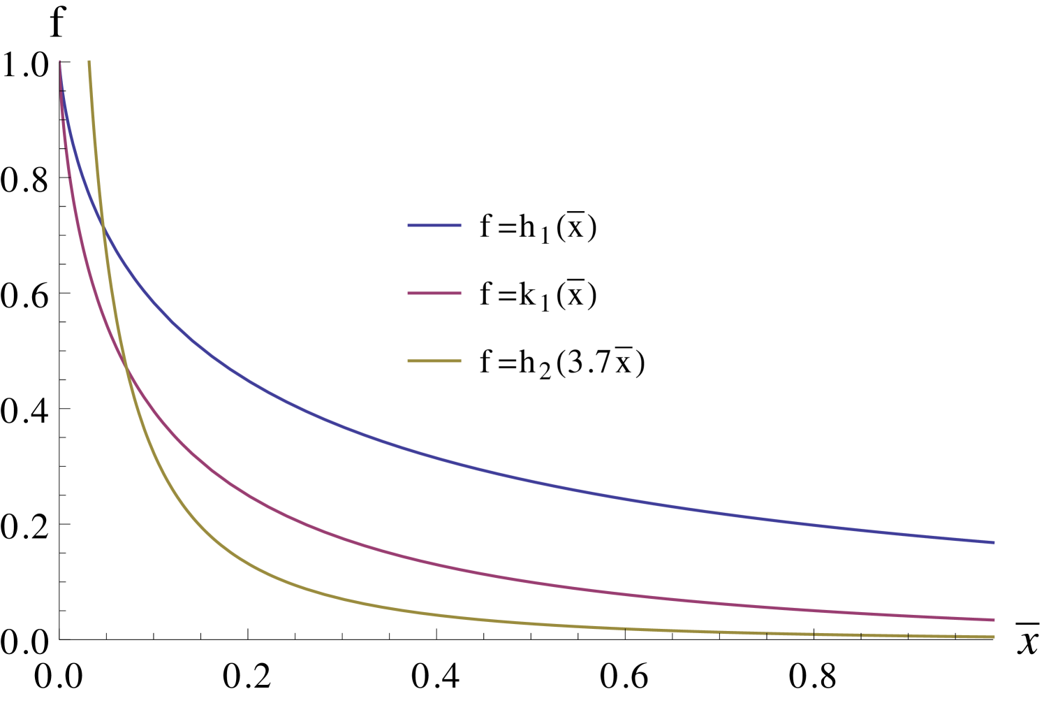
where and are given in Eq. (A.12). Moreover for and with the latter being defined in Eq. (A.12). The expression of Eq. (4.4) is actually proportional to the bino mass , which we have approximated by Eq. (4.2) using . The dimensionless loop functions , whose expressions can be found in Appendix B encode the contributions from the pure bino () and the bino-higgsino with left- () and right-handed () slepton diagrams. For , all ratios of different functions are close to one. With increasing , takes slightly larger values than the rest of the functions, reaching up to twice the value of and three times the value of . This can be seen in the limit where the left- and right-type slepton masses are not very different, such that the loop functions take the form [41]
| (4.5) |
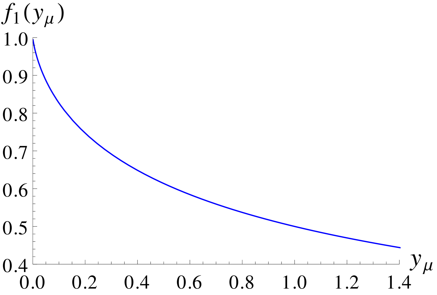
where we consider as the average slepton mass999 and only differ in the order one coefficients and which take values in the same range. Since the dominant term in Eq. (4.4) involves the first generation masses, we use rather than as the average slepton mass. and . The function is given in Appendix B while denotes the derivative . Their behaviour is shown in the right panel of Figure 4.
The dominant contribution to the electron EDM comes from the single chirality flipping diagonal mass insertion , such that we can make the approximation
| (4.6) |
where is an RG running factor defined in Eq. (3.9) and , defined in Eq. (A.2), is the (11) element of , with denoting the GUT scale soft trilinear matrix in the SCKM basis. Its imaginary part is non-zero when allowing the phases of the soft trilinear sector to be different from the phases of the corresponding Yukawa sector. Then, for , TeV and , we expect to vary around .
As can be seen in the left panel of Figure 4, which was produced using the full expression in Eq. (4.4), the numerical choice for the suppression factor corresponds to the yellow points and brings our prediction for the EDM above its current experimental limit, represented by the red dotted line.
In the case where the phases of the soft trilinear and Yukawa sectors are equal, and all factors in Eq. (A.2) become real. In that case, the dominant imaginary part originates from the NLO contribution101010The SCKM rotation which renders the Yukawa sector diagonal and real does not do the same to the -terms beyond leading order. to and is proportional to . Setting , as is preferred by the Jarlskog invariant , given in Eq. (2.20), we see that also the NLO contribution vanishes for , such that would only arise at order .
Concerning the terms of Eq. (4.4) with double mass insertions, they enter at orders , and in our model. In the situation described in the preceding paragraph, the first two terms are real, while the contributions of the latter two cancel against each other. Finally, the contributions of the triple mass insertions are further suppressed, with the largest one, , being real in the case at hand, while all other triple insertions entail contributions which lie below the experimental limit.
4.2
According to Figure 3, a large part of our parameter space in the (12) charged lepton sector appears to be excluded by the experimental limit set by the non-observation of . In this section, we therefore study in detail the contributions to this LFV process within our model. The current experimental limit for the branching ratio
| (4.7) |
is set by the MEG collaboration [43]. The expression for the corresponding SUSY contribution is given by [41]
| (4.8) | |||||
It is proportional to the bino mass squared, that has been approximated by Eq. (4.2) and expressed as , where . The loop function encodes the wino-higgsino contribution and is defined in Appendix B, along with the rest of the functions .
In our model, , , and . To get an estimate of the dominant s in Eq. (4.8), we first compare the () and the () contributions to the term by studying the ratio
| (4.9) |
which, in the limit where and are not very different, can be written as
| (4.10) |
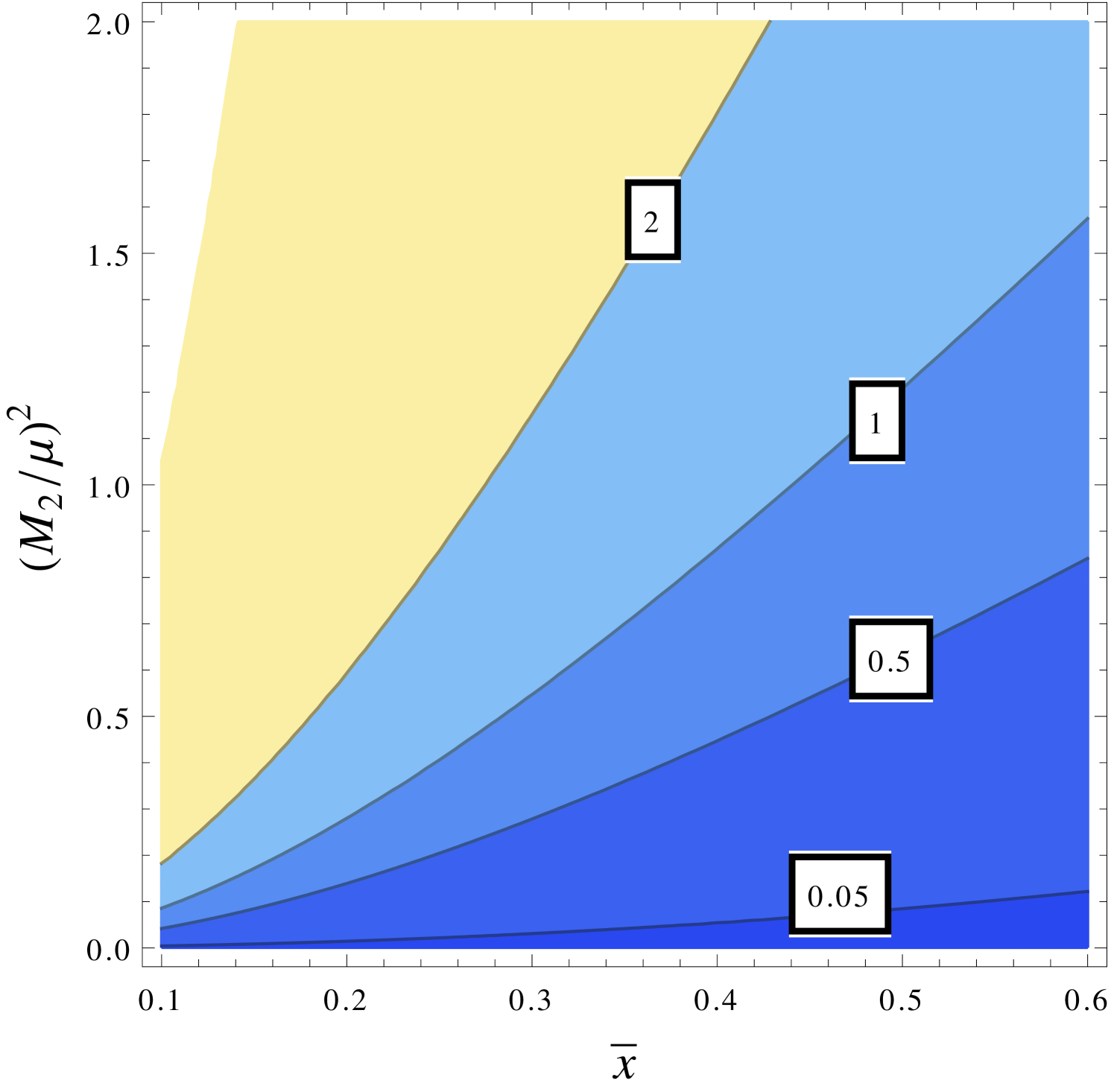
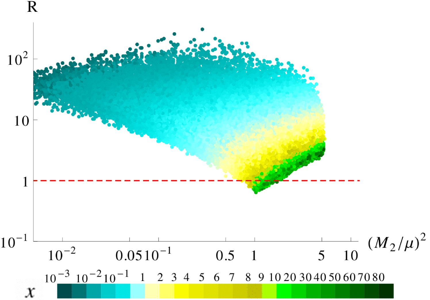
The behaviour of the loop functions and , which are defined in Appendix B, as well as is shown in the right panel of Figure 4, and , , , with . The contours in the left panel of Figure 5 show the dependence of , as defined in Eq. (4.10), on and . We see that for , is larger than one for all , while for and smaller, the contributions can dominate if does not decrease faster than . The right panel in Figure 5 is based on our scan and shows that the correlation of and through is such that , as defined in Eq. (4.9), stays larger than one in most of our parameter space, making the contribution to the term in Eq. (4.8) the most important one.
Similarly, one can show that the contribution to in Eq. (4.8) is comparable to the one only when , although is suppressed by an order of with respect to . This happens because the parameter has only two contributions which come in with opposite signs, allowing even for a complete cancellation.
Finally, we study the relative size of the and contributions by considering the ratio
| (4.11) |
where , with , , , and defined in Eqs. (A.1,A.2,A.15,A.54,2.33), respectively. The absolute value of the right-hand side of Eq. (4.11) exhibits a similar behaviour as the ratio , defined in Eq. (4.9) and shown in the right panel of Figure 5. Taking into account the -suppression () and the range of which can vary within two orders of magnitude, we find that the contribution to the branching ratio can be comparable to the one when .
Considering situations in which the contribution to Eq. (4.8) dominates, we obtain the approximate expression
| (4.12) |
In the case where is more important, e.g. when , cf. right panel of Figure 5, we obtain
| (4.13) |
For , , , , TeV and GeV, the approximations of Eqs. (4.12,4.13) both produce a value of the order of times the relevant order one coefficients squared. In order to gain an extra suppression of at least an order of magnitude, the latter are preferred to be smaller than one.
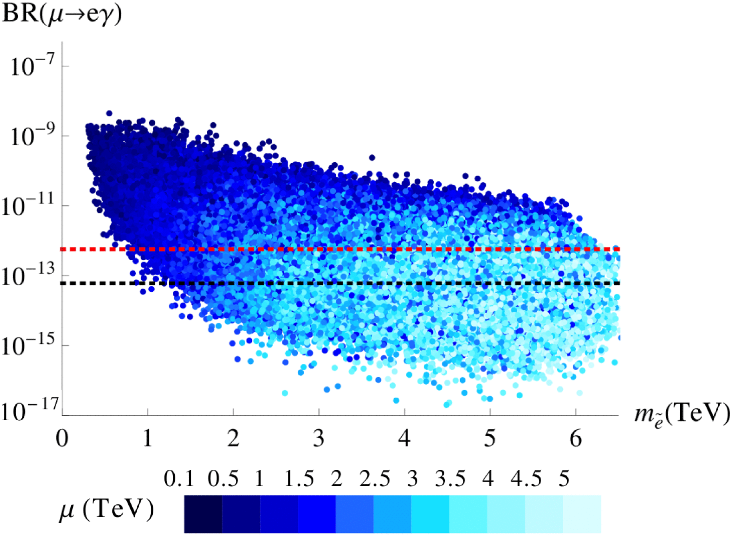
The total supersymmetric contribution to the branching ratio of of Eq. (4.8) as produced in our scan is shown in Figure 6. There it is plotted against the average slepton mass (left panel) as well as (right panel). From the left panel we observe that our model requires rather heavy sleptons, in the TeV range, in order to survive the current experimental limit in Eq. (4.7), which is denoted by the red dotted line. As can be seen in Eqs. (4.8,4.13), there is also a strong dependence, with a preference for large values. The right panel of Figure 6 shows that the branching ratio is correlated with the electron EDM, mainly through the slepton masses and the bino-slepton mass ratio. The combination of the current limits on both observables highly restricts our parameter space. Reaching the expected future limits, denoted by the black dotted lines, would nearly exclude our model.
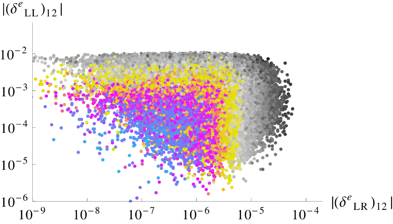
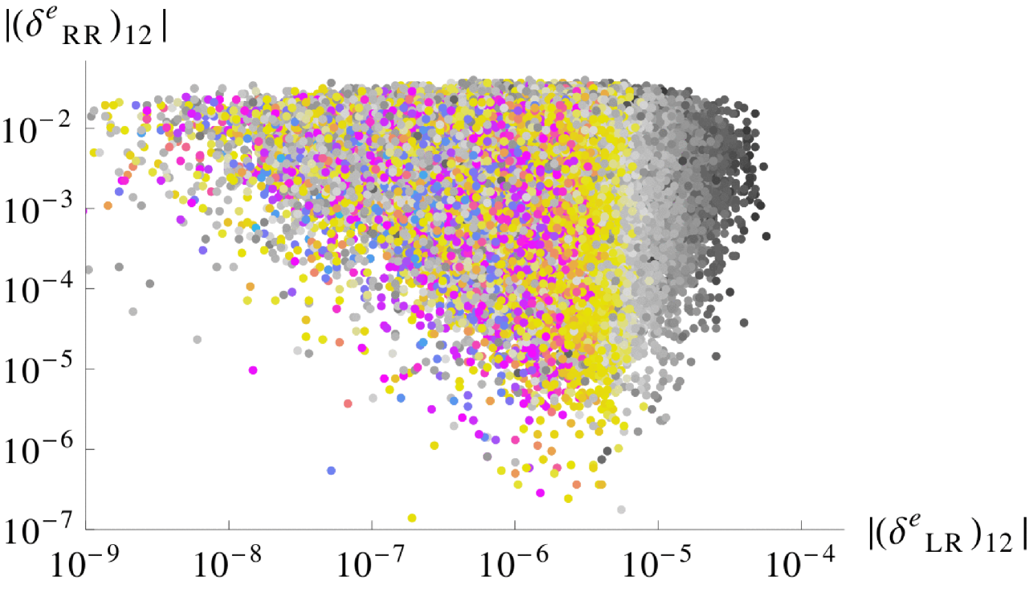
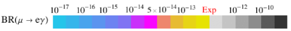
In Figure 7 we show our predictions for in the plane of two (12) mass insertion parameters as produced in our scan. Comparing this to the discussion of Section 3.2.3 reveals that, with the present MEG bound, and are not excluded as it was suggested by the limits in Figure 3. On the other hand, can take its maximum values produced by the scan. The reason for these weaker bounds is twofold. Firstly, the analysis in [38] sets the limits on the mass insertion parameters by choosing as large as 60, whereas we only allow for maximum values of 25. Secondly, the derivation in [38] requires that the discrepancy of from its SM value is explained by SUSY contributions.
4.3 Meson mixing
Turning to transitions, we study the SUSY contributions to meson mixing. The dispersive part of the mixing for a meson can be parametrised as [45]
| (4.14) |
and the corresponding mass difference is given by
| (4.15) |
We express the SM contribution as . The New Physics (NP) contribution, , is encoded in the real parameters
| (4.16) |
The contributions of the gluino-squark box diagram in terms of mass
insertion parameters read [11, 15]
| (4.17) | |||||
where
| (4.18) | |||||
denotes the mass of the meson under consideration and is the associated decay constant. and are the masses of the meson’s constituent quarks while is an average squark mass which we define as
| (4.21) |
with , and defined in Eq. (A.11). The loop functions and , where , are given in Appendix B and the gluino mass has been approximated by Eq. (4.2).
4.3.1 mixing
The SM contribution to , meson mixing given by [46]
| (4.22) |
with
| (4.23) | |||||
| (4.24) |
Here is a QCD factor, a perturbative parameter related to hadronic matrix elements and is the Inami-Lim loop function [47]. The calculation of the pure SM contribution to the mass difference gives [48]
| (4.25) |
with the largest uncertainty stemming from the non-perturbative factor , for which the value MeV [49] has been used.111111We note that the 2014 average of the FLAG collaboration [50] corresponds to a lower central value but with a larger error: . The SM prediction for can be deduced from the ratio [48]
| (4.26) |
which is less sensitive to theoretical uncertainties. On the other hand, the associated experimental averages as of summer 2014, provided by the HFAG group, read [51]
| (4.27) | |||||
| (4.28) | |||||
| (4.29) |
Comparing Eq. (4.25) with Eq. (4.27) leads to a negative central value for the experimentally allowed NP contribution to , with a similar result being obtained for . The main source for the errors are the uncertainties of the SM calculation.121212For a recent discussion on theoretical uncertainties and comparison with experimental results, see [52]. In view of Eqs. (4.25-4.29), and in anticipation of reduced theoretical uncertainties, we conclude that the largest NP effects that could still be allowed should be consistent with
| (4.30) |
Using Eqs. (4.15,4.17), we can estimate the effects of the gluino-squark box diagrams. Taking into account the -suppression of each parameter entering Eq. (4.17), we can write in the schematic form
| (4.31) |
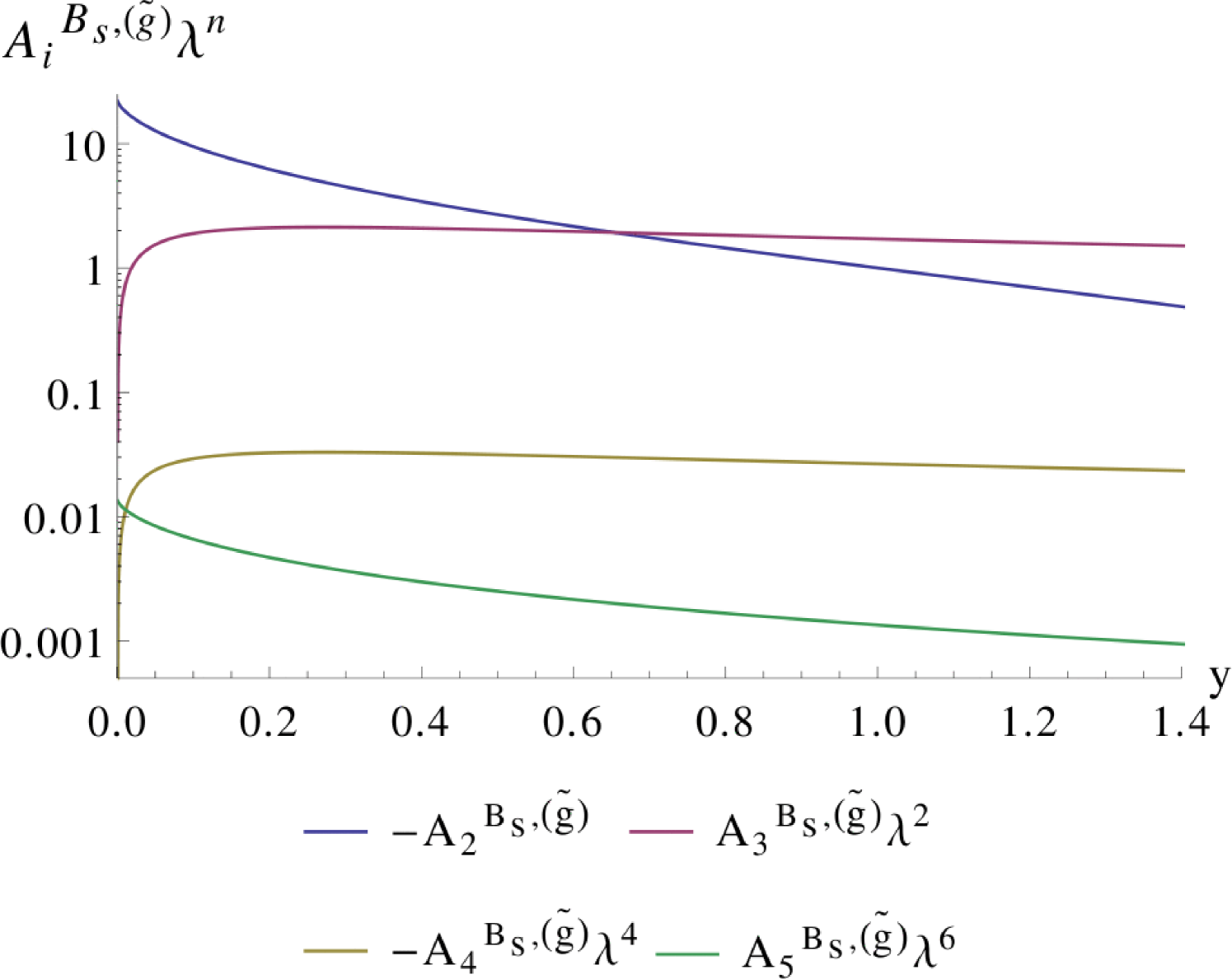
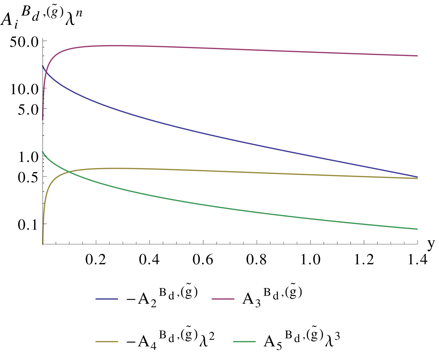
Figure 8 shows the individual contributions as a function of . The largest contributions originate from the terms proportional to and , i.e. the terms associated with the and , cf. Eq. (4.17). The contributions from the -type mass insertion parameters, proportional to , are negligible. The maximum effect of the gluino-squark box diagrams is obtained when and are smaller than one, with the and terms interfering constructively. For relatively light around 2 TeV, GeV. Assuming furthermore , and (cf. Figure 2) as well as , we can use Eqs. (4.15,4.17) together with Figure 8 to estimate the maximum gluino effects as GeV and GeV. This is about two orders of magnitude smaller than the corresponding SM and experimental values.
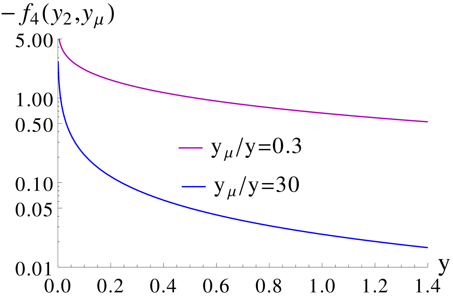
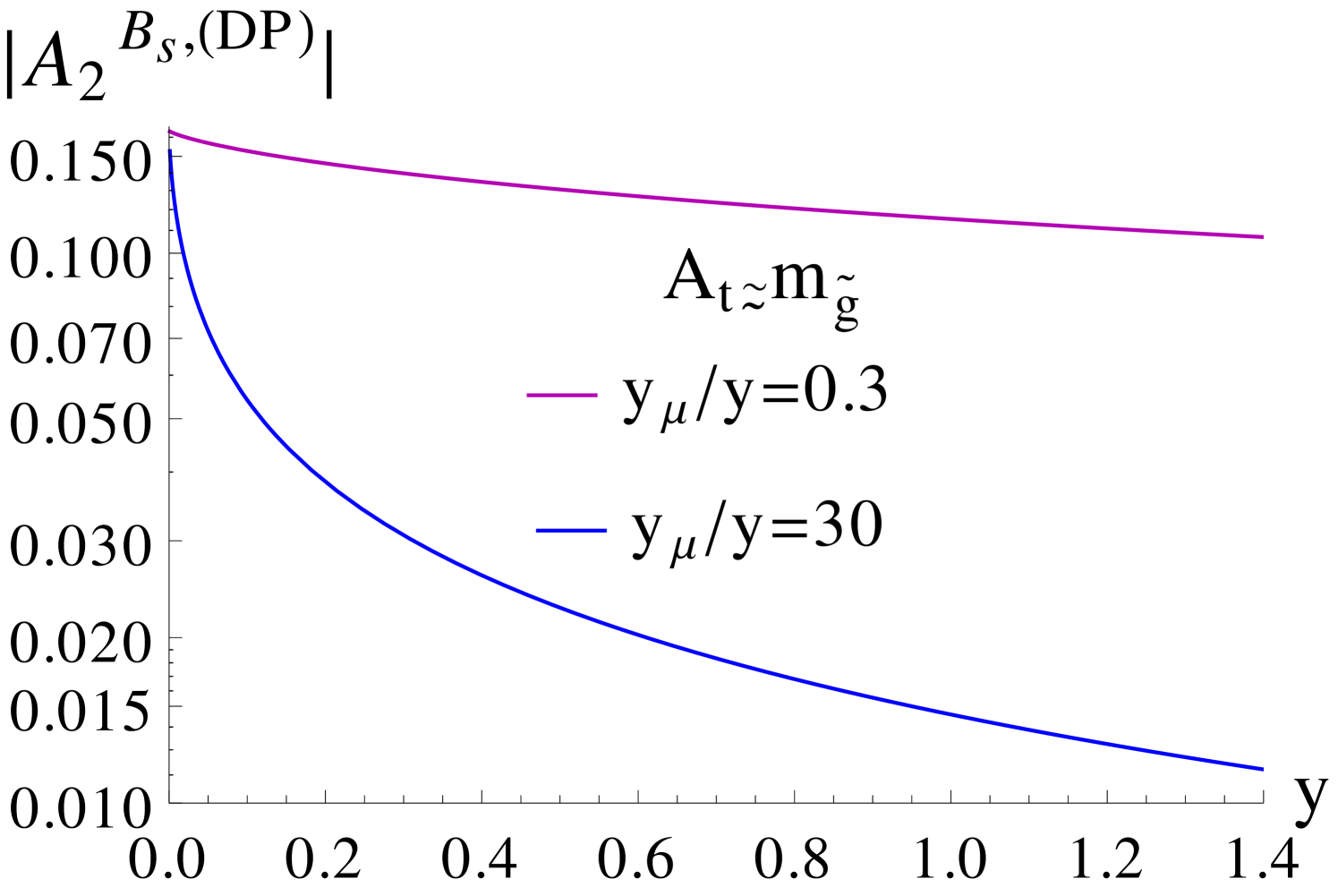
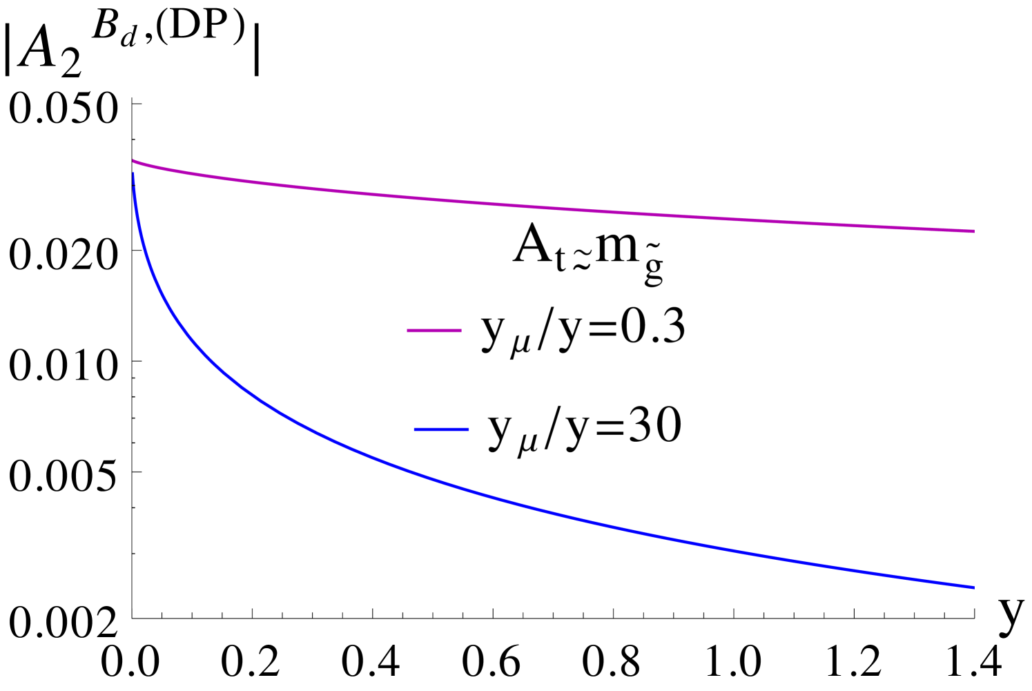
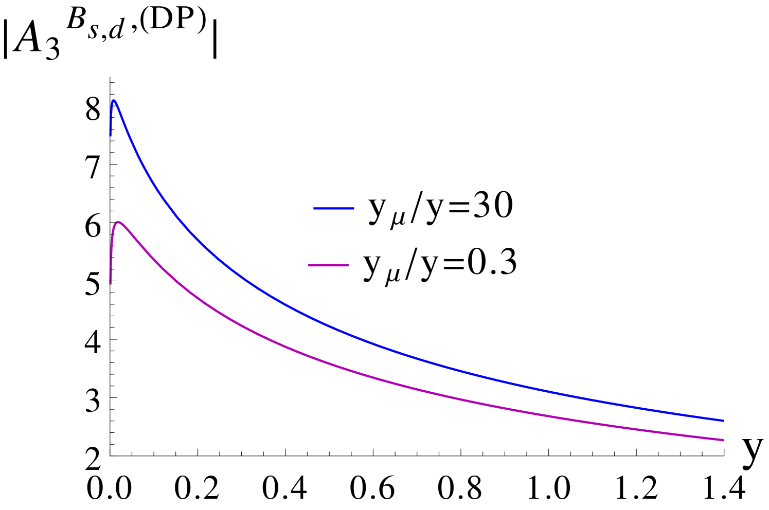
For relatively large values of and a light CP-odd Higgs mass , the contributions of the double penguin (DP) diagrams, which scale as , become important. Considering diagrams with () two gluino, () one gluino and one Higgsino and () one gluino and one Wino loops, the associated part of can be approximated by [15]
| (4.32) |
where for and
| (4.33) |
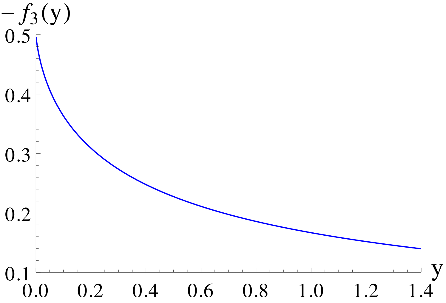
and where the latter is related to via the approximations of Eq. (4.2). The loop functions , , are given in Appendix B. Their behaviour is sketched in Figure 9, along with that of . For GeV, the dominant contribution to Eq. (4.32) comes from in the sector, even for our maximum values of , while for , where assumes larger values (cf. Figure 2), the two terms in the curly brackets are comparable. For light average squark masses around 2 TeV, can reach values up to GeV, while (cf. Figure 2). Then, for and , , such that GeV, barring contributions from the term. When takes its maximum value of 25 and , the double penguin contributions to increase to about an order of magnitude above the gluino-box contributions, which is however still significantly below the SM and experimental values.
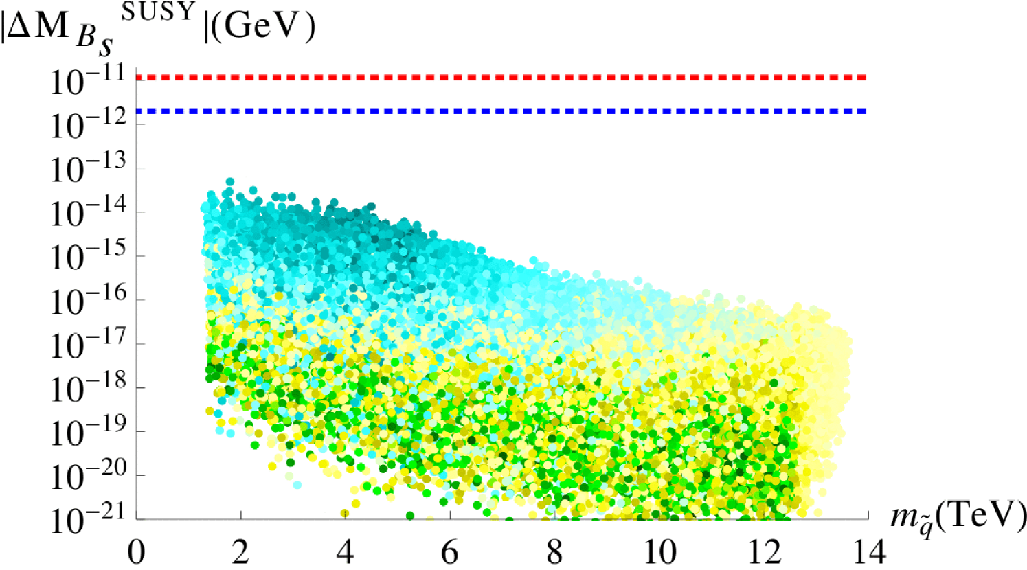
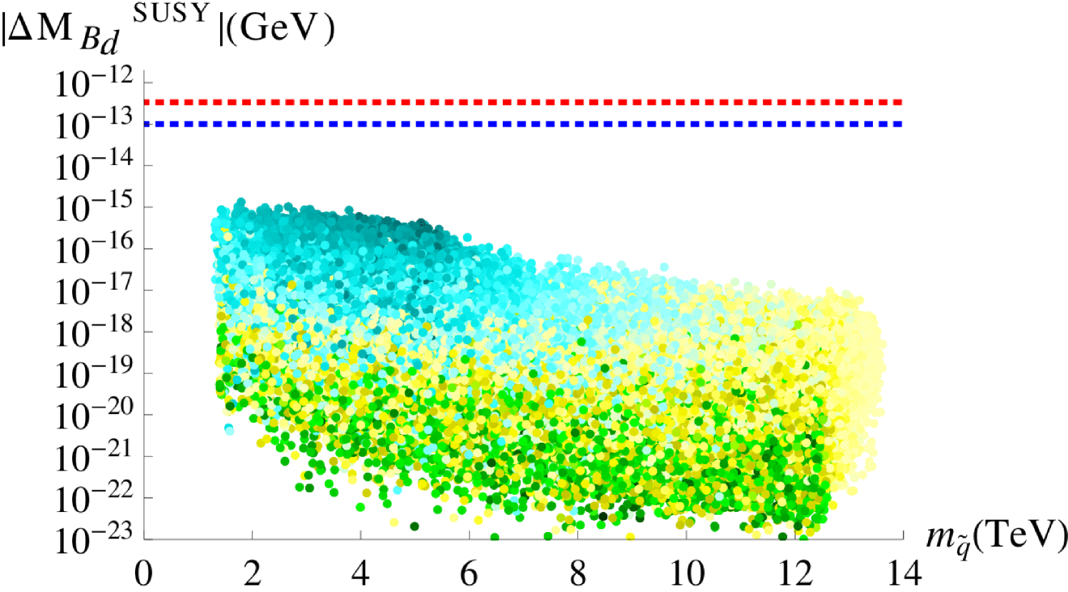
Figure 10 shows the predicted SUSY contributions to the meson mixings as produced in our scan. They are plotted against the average squark mass defined in Eq. (4.21) and lie below both the experimental measurements (red dotted lines) and the NP limits (blue dotted lines) by at least an order of magnitude. This result is in agreement with the findings in Section 3.2.2, where we have compared our predictions for the mass insertion parameters with existing limits in the literature.
The effects of the complex down-type mass insertion parameters of the (23) and (13) sectors can be studied through the time dependent CP asymmetries associated with the decays and . Focusing on the mixing-induced CP asymmetries, we have [53]
| (4.34) |
with
| (4.35) |
where denotes the final state of the decay and is the corresponding amplitude. As the absorptive part of the meson mixing is much smaller than the dispersive one , i.e. , we can approximate . Then, the factors associated with the decays and take the form
| (4.36) |
where the parameters and are defined in Eq. (4.16), while the SM phases and can be found in Eqs. (4.23,4.24). The mixing-induced time dependent asymmetries can then be simply written as
| (4.37) |
The current measurements are [51]131313LHCb recently published their first measurements of [54] in the limit of a vanishing direct CP asymmetry, i.e. , thereby improving consistency with the SM expectation.
| (4.38) |
while the SM expectations read [55]
| (4.39) |
comes with a relatively small error, whereas depends strongly on the value of , which differs significantly when extracted via inclusive or exclusive decays, see e.g. [46], with the above data preferring the lower exclusive result. The value of quoted in Eq. (4.39) has been derived by averaging over inclusive and exclusive semileptonic determinations of the relevant CKM elements and using the value of the CP-violating parameter , see Eq. (4.47), amongst the input parameters but not the measurement of itself.
Comparing Eq. (4.38) and Eq. (4.39), we observe that the NP contributions to and can be as large as and of the respective SM values. In order to reach deviations, and should be larger than and respectively, corresponding to . Here we have assumed NP phases which maximise the effect. In view of Figure 10, we would expect a non-negligible contribution to in a small part of the parameter space. However, at leading order, and are real, cf. Eqs. (A.31,A.33). They only receive non-trivial phase factors at order , suppressing the imaginary part of by one power of with respect to the real part. As a result, any deviation from is only of the order of . In the sector, and are already complex at leading order in , cf. Eqs. (A.30,A.32). But as can be seen from Figure 10, is too small to be relevant. Even for , the maximum deviation from would be at most.
In conclusion, our model would not be able to explain any persistent deviations from SM expectations in observables related to meson mixing.
4.3.2 mixing
The SM contribution to the Kaon mixing reads [46]
| (4.40) | |||||
where are QCD factors, denotes a perturbative parameter and are the Inami-Lim loop functions [47]. From this, the SM value for the Kaon mass difference is numerically given by [56]
| (4.41) |
while the experimental measurement yields [57]
| (4.42) |
We therefore impose the constraint that the maximum allowed NP contribution should be limited by
| (4.43) |
For Kaon mixing, the relevant mass insertion parameters are those of the (12) sector. Taking into account their -suppression, we can write the gluino-box contribution to the mixing amplitude, given in Eq. (4.17), in the schematic form
| (4.44) |
Figure 11 depicts the individual contributions as a function of . It shows that the dominant contribution originates from the term proportional to , i.e. the term proportional to , see Eq. (4.17). The effects of the -type s, proportional to , are negligible. Using Eqs. (4.15,4.17) together with Figure 11, we can estimate the maximum gluino contributions to . Assuming , GeV and , (cf. Figure 2), we expect that GeV, which is about one order of magnitude larger than the experimental result of Eq. (4.42).
The double penguin (DP) contributions to arise at the level of four mass insertions, by effectively generating the transitions through followed by . The relevant part of the mixing amplitude takes the form [15]
| (4.45) | |||||
| (4.46) |
with the loop function given in Appendix B. We find that this contribution is completely negligible, as it is proportional to . The upper left panel of Figure 12 shows the combined gluino and DP SUSY contribution to , as produced in our scan. It can exceed the NP limit quoted in Eq. (4.43) (blue dotted line) for small values of , even shooting above the experimental value of Eq. (4.42) (red dotted line) for .

We now turn to the CP-violating parameter , defined as [46]
| (4.47) |
where the superweak phase141414 denotes the difference of the widths. [57], and the factor [58] takes into account that and includes long distance contributions. The experimentally measured value of is [57]
| (4.48) |
while the SM prediction depends highly on the value of [46]. According to [59] and for the input set from the angle-only fit [60], where the Wolfenstein parameters do not show an unwanted correlation with and , one finds
| (4.49) |
We therefore demand that
| (4.50) |
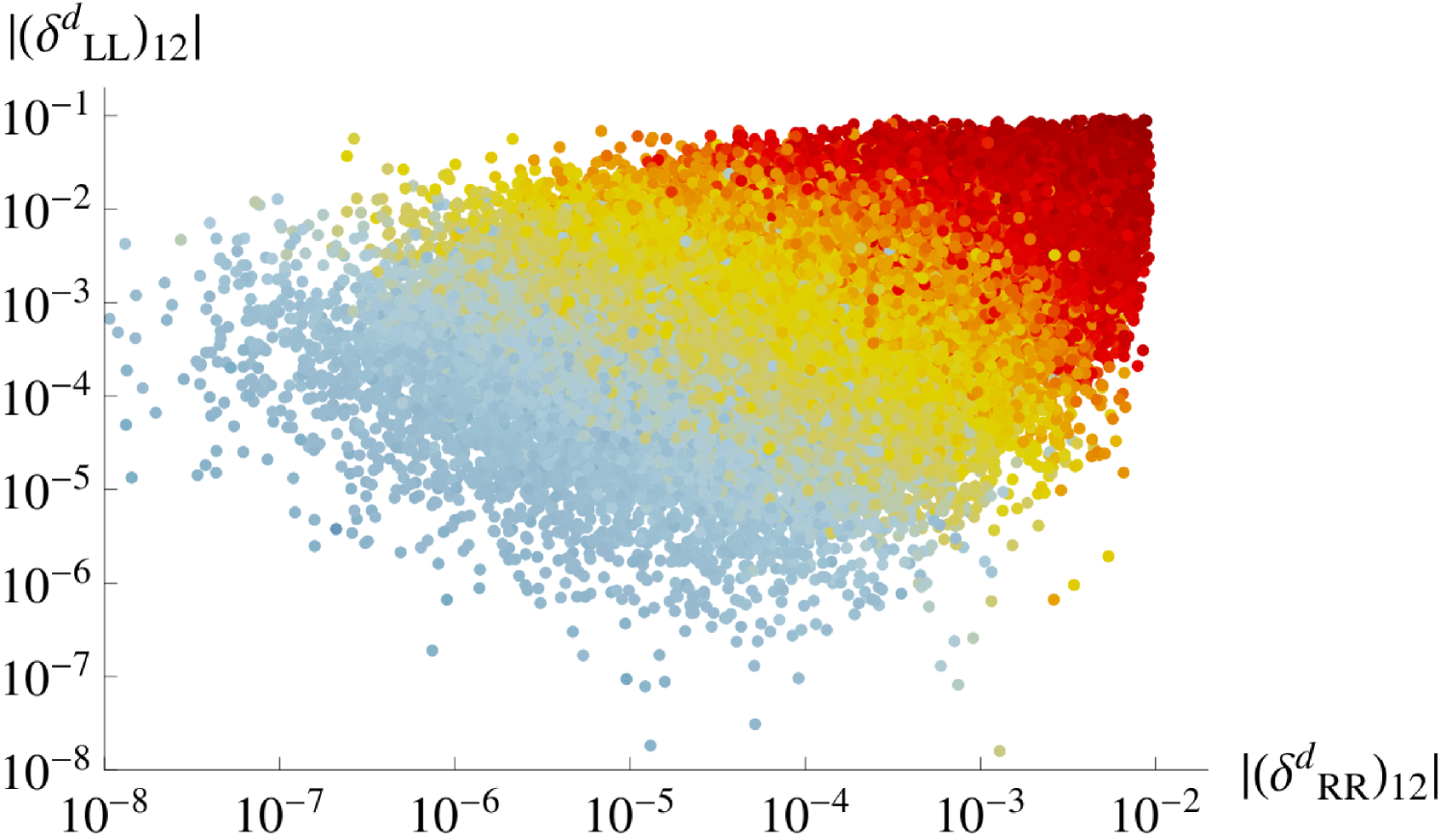
The upper right panel of Figure 12 shows the absolute value of our predicted SUSY contribution to , plotted against the average squark mass. We find that it can exceed the limit of Eq. (4.50) by more than three orders of magnitude when . In view of Figure 2, we would not have expected such a big effect. However, the limits on the mass insertion parameters used in Section 3.2.2, only take into account one non-zero mass insertion at a time. As we have seen in this section, the dominant contribution to the Kaon mixing amplitude stems from the multiple term (cf. Figure 11). The non-zero phase of the parameter is the source of our prediction of a large .
The lower left panel of Figure 12 shows in the plane. It indicates that for , i.e. towards the largest possible value according to Figure 2, is required. When takes its maximum value of , should stay below .
Finally, from the lower right panel of Figure 12 we observe that places stronger bounds on the mass insertion parameters than . Due to the framework of our model there is a correlation between the parameters relevant in Kaon mixing and the ones that enter the branching ratio of . Denoting the points excluded by with a grey shade reveals that there still remains a small area of parameter space which is excluded by .
4.4
We now consider the gluino contribution to the branching ratio of . In terms of the relevant mass insertion parameters it is given by [11]
| (4.51) |
where the loop functions are defined in Appendix B, denotes the mean life of the meson and . This observable does not constrain our parameter space. Even for squark masses as low as 100 GeV and , the and mass insertion parameters would only need to be smaller than 0.4 to be consistent with the current experimental value of [51]
| (4.52) |
which is in good agreement with the SM prediction [61]. Similarly, the chirality flipping mass insertion parameters would need to be smaller than . In our scan we find, cf. Figure 2, , , and . Taking into account the squark mass dependence and the fact that our scan excludes such light squarks, we have found that our model predicts a contribution to which is at least three orders of magnitude below the experimental measurement.
4.5
The most recent SM predictions for the branching ratios of are given by [62]
| (4.53) |
while the averages of the CMS and LHCb collaborations read [63]
| (4.54) |
The sector therefore still allows for rather large relative deviations from the SM expectations. In the case of the experimental measurement yields a value which is slightly lower than the SM prediction.151515The calculations in [62] have been performed using the inclusive value of . Working with the exclusive one would result in a lower central value of which fully agrees with the data [64]. We therefore quote the allowed room for contributions from new physics as
| (4.55) |
The chargino and gluino contributions to the branching ratio of can be expressed as [15]
where
| (4.57) |
with and for . The loop functions , and are the ones which appear in the double penguin contributions to mixing in Section 4.3.1. With and GeV, the dominant contribution to Eq. (4.5) originates from the flavour blind term of , such that we can make the approximation
| (4.58) |
Then, for , TeV, and receiving its maximum value of order one (cf. Figure 9), we expect .
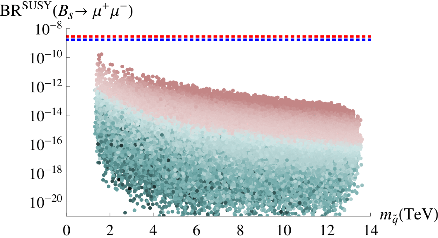
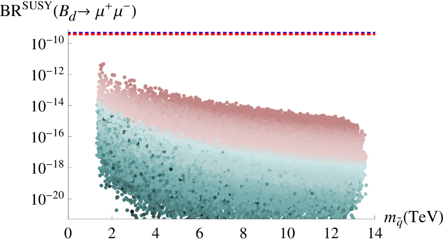
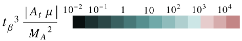
In Figure 13, we plot our predicted SUSY contributions to the branching ratios of against the average squark mass , defined in Eq. (4.21). The red dotted lines denote the experimental measurements, while the blue ones correspond to the limits for the NP contributions as given in Eq. (4.55). In both sectors, and , our maximum predictions fall about an order of magnitude below these limits.161616As discussed in [65] and also in [66], the theory prediction in Eq. (4.5) should take into account the large width difference between the mass eigenstates of the system. This correction enhances the corresponding branching ratio by about 10%. Given the smallness of the new physics contribution in our model, it does, however, not change our results significantly.
4.6 Neutron and 199Hg EDMs
CP-violating effects in the quark sector can manifest themselves through the quark EDMs as well as the quark Chromo Electric Dipole Moments (CEDMs). The gluino contributions read [67, 68, 15]
| (4.59) |
with
| (4.60) |
where denotes the electric charge of quark and the loop functions , , with , are given in Appendix B. As the first generation squarks dominate Eq. (4.59), we use the average squark masses
| (4.61) |
Similar to the case of the electron EDM, we consider the most general scenario
where the phases of the soft trilinear sector are different from the
corresponding Yukawa ones. Then the dominant contributions of Eq. (4.59)
arise from the single mass insertions with ,
| (4.62) |
where is defined in Eq. (A.2). The double and triple mass insertions start contributing at orders and for the up and down quark (C)EDMs, respectively.
If, however, the phases of the soft trilinear and Yukawa sectors are aligned, is real. In the case of the up quark sector, one should then check171717We have truncated our expansion at the order of . whether the NLO corrections to also vanish, before assuming that the term dominates. The situation in the down sector is such that the NLO correction to gives a non-vanishing contribution to the (C)EDMs. Explicitly, we find , while the smallest contribution from multiple mass insertions is .
In order to compare the gluino contributions of our model according to Eq. (4.59) with the experimental limits, we take into account the RG running from the SUSY scale down to the hadronic scale, using the LO results of [69], for and [70]. Then,
| (4.63) |
with as given in Eq. (4.59).
With these preparations, we can study the predictions for the neutron and the 199Hg EDMs. Adopting the QCD sum rules approach, the neutron EDM at the renormalisation scale GeV is given in terms of the QCD -term and the quark (C)EDMs by [42]
| (4.64) |
while the current experimental limit is [71]
| (4.65) |
The quark (C)EDMs can also be probed through measurements of the EDMs of atomic systems, where 199Hg provides the best upper limit amongst the diamagnetic systems [72]
| (4.66) |
However, large theoretical uncertainties in the atomic and in particular the nuclear calculations prevent the extraction of bounds on . Eq. (4.66) limits the nuclear Schiff moment as [73]
| (4.67) |
which, assuming it is dominated by pion-nucleon interactions, can be expressed as [74]
| (4.68) |
In this equation, the denote the pion-nucleon couplings. Their coefficients in Eq. (4.68) are the best fit values taken from the review article [74], which assesses the strengths and weaknesses of different, sometimes contradictory, nuclear calculations provided in the literature. Combining Eqs. (4.67,4.68) with the relation
| (4.69) |
which was derived in [75], it can be inferred that [73]
| (4.70) |
However, this bound only applies if the coefficient of in Eq. (4.68) takes its best fit value. In principle, it could also be zero, in which case no bound on could be extracted.
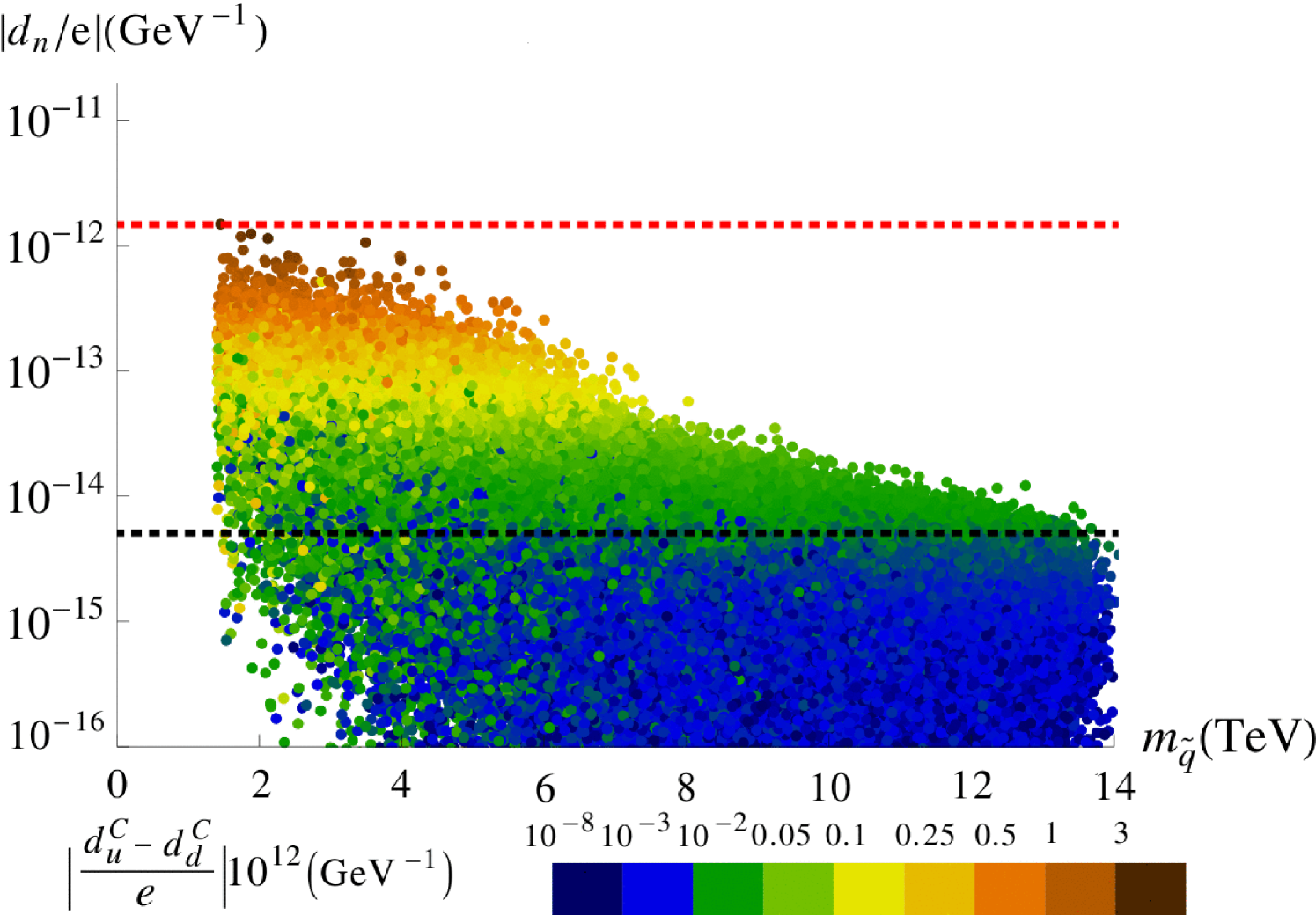
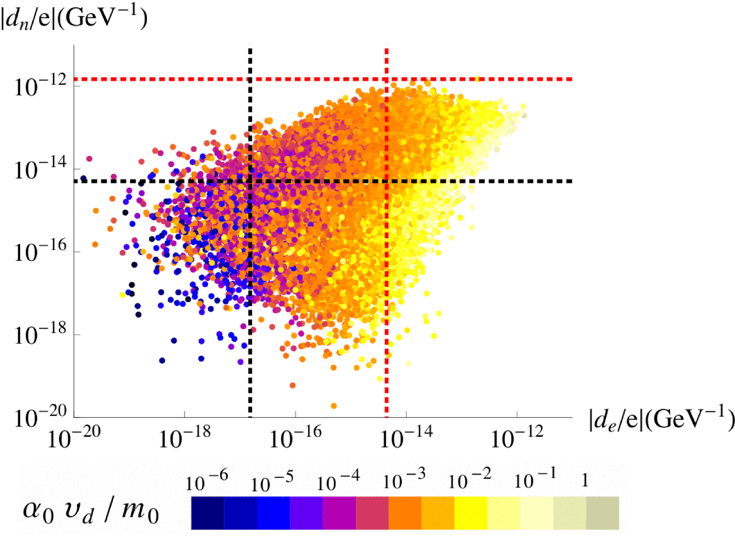
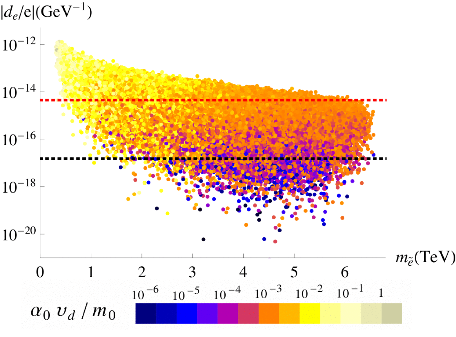
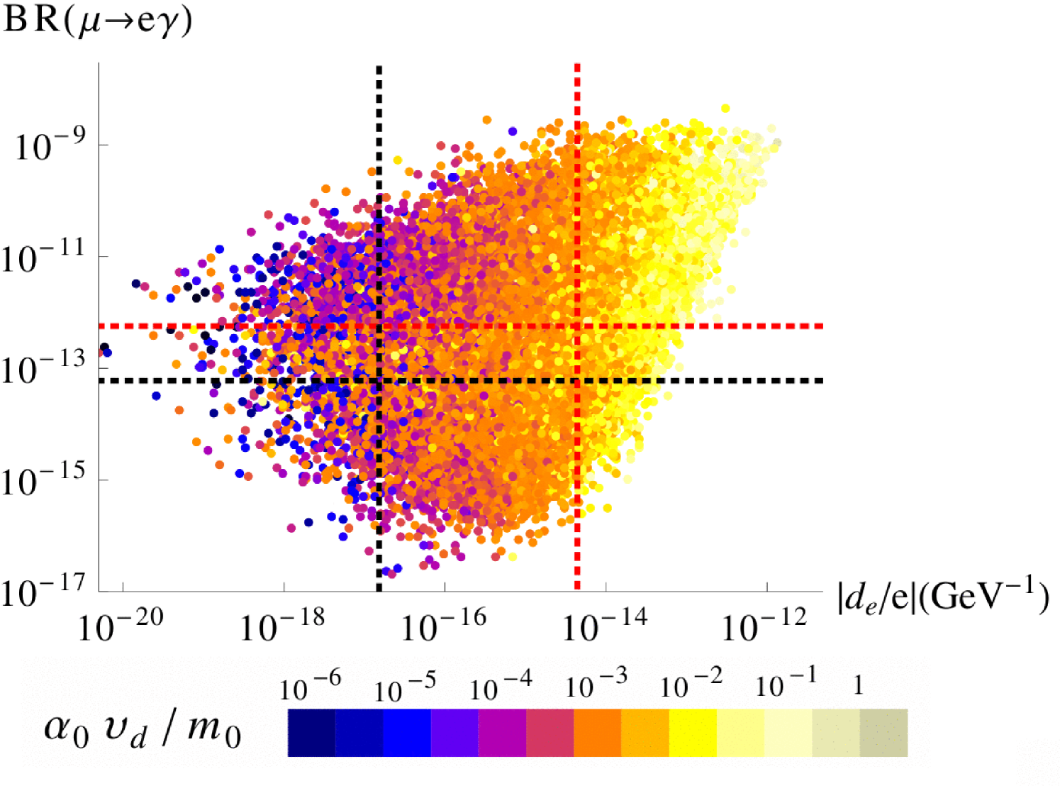
In the left panel of Figure 14, we show our prediction for the neutron EDM versus the average first generation squark mass . For squark masses less than about 6 TeV, it lies just below the red line denoting the experimental limit in Eq. (4.65). For heavier squarks it stays below the limit by at least one order of magnitude. The colour coding corresponds to the predicted value of GeV, which can also reach the limit in Eq. (4.70) for large values. In the right panel of Figure 14, the neutron and electron EDMs are plotted against each other. They are of the same order of magnitude, but it is the current electron EDM limit that constrains our parameter space. When the future experimental limits are reached, only the small part lying in the lower left corner bounded by the black dotted lines will survive.
5 Conclusions
In a recent paper we showed how MFV can emerge approximately from an SUSY GUT whose flavour structure is controlled by the family symmetry [1], providing a good description of all quark and lepton masses, mixings as well as CP violation. We showed that the model leads to mass insertion parameters in Eqs. (2.43,2.53,2.63) which very closely resemble the MFV forms, where are unit matrices and are proportional to the Yukawa matrices.
Whereas in [1] we focused on the similarity to MFV, here we highlight the differences, which we do by considering the predictions for electric dipole moments, lepton flavour violation, and meson mixing as well as rare decays. As expected, many of the new physics contributions fall well below current limits. This is the case for example in physics observables, where deviations are negligible (at the 1% level). Thus, our model would be unable to explain any discrepancies between SM expectations and measurements in or in the time dependent asymmetries and . This is in marked contrast to the family symmetry models previously studied, where large effects were expected in these observables. Thus, neutrino physics which led to , appears to lead us towards models with small such deviations.
On the other hand there are observable effects which would distinguish the SUSY GUT model from MFV. The most significant effects of the departure from MFV appear in the (12) down-type quark and charged lepton sectors, related to Kaon mixing observables and the branching ratio of . We find that provides the dominant contribution to BR() and that our model requires rather heavy sleptons, exceeding about 1 TeV, in order to satisfy the experimental bound. Another important area where our model gives observable deviations from MFV is CP violation, in particular the electron EDM, where again large (TeV scale) slepton masses are required for compatibility with current bounds to be achieved. The model therefore predicts that a signal should be observed in both and the electron EDM within the expected future sensitivity of these experiments.
Turning to CP violation in the Kaon system, the model contributes significantly to due to the phase of . The SM prediction for this observable depends sensitively on , which differs when considering inclusive or exclusive decays, leading to a lower central value in the latter case. However, even for inclusive values of , the SM expectation for is about 10% below the measurement. Our model is capable of providing sufficient enhancement to explain the experimentally observed value of .
We collect our findings in Table 7, where we classify various flavour observables according to the expected size of our model’s predictions. Large observable effects are indicated by , while visible but small effects are labelled by . A single star shows the absence of sizable effects on a particular flavour observable. This classification, which was first suggested in [15], is undoubtedly somewhat vague by nature and therefore limited in its scope. Yet, it has proved to be a useful tool in comparing characteristic predictions of various models of flavour. Table 8 of [15] shows the expected predictions of a selection of different models. Comparing this table with our model’s DNA, see Table 7, demonstrates the specific signatures of our SUSY GUT of flavour. According to the phenomenological study in [15], all of the discussed models which predict large effects on also predict large contributions to . In contrast, our model features large contributions to in conjunction with negligible effects on . Furthermore, all SUSY models in [15] entail large contributions to while such contributions are tiny in our model. Those models in [15] which lead to a large electron EDM () also predict a large neutron EDM (). Again, our model differs from this pattern by predicting large observable together with only small . Concerning we observe that sizable effects are expected for our model as well as all flavour models scrutinised in [15]. This comparison illustrates that the phenomenological signatures of our SUSY GUT are indeed quite different from those of previously discussed flavour models.
In summary, theories with discrete flavour symmetries such as the SUSY GUT model, motivated by neutrino physics, seem to lead to MFV-like flavour changing expectations, but with some important exceptions. This study shows that, while observable deviations in physics are generally not expected to show up, departures from MFV are expected in both and the electron EDM within the foreseeable future sensitivity of these experiments. CP violating effects may also be observed in , perhaps resolving some possible SM discrepancies.
Acknowledgements
We thank Claudia Hagedorn for helpful discussions throughout this project. MD and SFK acknowledge partial support from the STFC Consolidated ST/J000396/1 grant and the European Union FP7 ITN-INVISIBLES (Marie Curie Actions, PITN-GA-2011-289442). CL is supported by the Deutsche Forschungsgemeinschaft (DFG) within the Research Unit FOR 1873 “Quark Flavour Physics and Effective Field Theories”.
Appendix
Appendix A Low energy mass insertion parameters
In this appendix, we show explicitly the full expressions of the low energy mass insertion parameters used in our numerical analysis. They are given in terms of the high energy order one coefficients introduced in Section 2. Performing the transformation to the SCKM basis, it is useful to define the corresponding GUT scale parameters
| (A.1) | |||||
and
| (A.2) |
Here, parameterises the (23) and (32) entries of the up-type quark Yukawa matrix of order before canonical normalisation; the associated phase is given by . They become subdominant contributions to the (23) and (32) elements of in Eq. (2.4). The parameter of the corresponding soft trilinear contribution is denoted by with phase . In addition to we also need which parameterises a subdominant contribution to the (22) and (23) elements of in Eq. (2.8) of order . For the phase we have , and the corresponding parameters of the -terms are and . It is worth mentioning that all become real in the limit where the Yukawa and trilinear phase structures are aligned such that the relation holds.
In order to describe the renormalisation group running from the GUT scale down to low energies, we introduce the parameters in Eqs. (3.8,3.9) as well as
| (A.3) | |||||
| (A.4) | |||||
| (A.5) |
and
| (A.6) | |||||
| (A.7) | |||||
| (A.8) | |||||
| (A.9) |
In these expressions, denotes the universal gauge coupling constant at the GUT scale, is the universal gaugino mass parameter and is the scale of the soft trilinear terms. Using the SUSY breaking mass , we have also introduced , see Eq. (3.13). and have been defined in Eq. (2.33), while is given in Eq. (3.12).
With these definitions, the parameter at the low energy scale can be approximated by , and the low energy sfermion masses, whose GUT scale definitions are given in Eq. (2.29), take the form
| (A.10) | |||||
| (A.11) | |||||
| (A.12) |
with
| (A.13) | |||||
| (A.14) | |||||
| (A.15) |
Here, as defined in Eqs. (3.13). With these definitions at hand, we can write the mass insertion parameters at the low energy as follows.
Up-type quark sector:
| (A.16) | |||||
| (A.17) | |||||
| (A.18) |
| (A.19) | |||||
| (A.20) | |||||
| (A.21) |
| (A.22) | |||||
| (A.23) | |||||
| (A.24) |
| (A.25) | |||||
| (A.26) | |||||
| (A.28) |
At the GUT scale, is zero up to the order where we truncate our expansion. The non-zero value in Eq. (A.26) is purely generated via the RG evolution. Similarly, a term proportional to is generated in , which was of order at the GUT scale. The -suppression of all other low energy mass insertion parameters remains unaffected by the running, such that the corresponding RG effects can simply be absorbed into new order one coefficients.
Down-type quark sector:
| (A.29) | |||||
| (A.30) | |||||
| (A.31) |
| (A.32) | |||||
| (A.33) |
| (A.34) | |||||
| (A.35) | |||||
| (A.36) |
| (A.37) | |||||
| (A.38) | |||||
| (A.39) | |||||
| (A.40) | |||||
Charged lepton sector:
Appendix B Loop functions
The dimensionless functions , , , , , and which appear in the expressions for the EDM of the electron in Section 4.1 and the branching ratio of in Section 4.2 are defined as [41]
| (B.1) |
where
| (B.2) | |||||
| (B.3) | |||||
| (B.4) |
| (B.5) | |||||
| (B.6) | |||||
| (B.7) | |||||
| (B.8) |
with
| (B.9) |
and
| (B.10) |
Note that we assume real and positive values for and .
References
- [1] M. Dimou, S. F. King and C. Luhn, JHEP 1602 (2016) 118 [arXiv:1511.07886].
- [2] S. F. King, Rept. Prog. Phys. 67 (2004) 107 [hep-ph/0310204]; G. Altarelli and F. Feruglio, Rev. Mod. Phys. 82 (2010) 2701 [arXiv:1002.0211]; S. F. King and C. Luhn, Rept. Prog. Phys. 76 (2013) 056201 [arXiv:1301.1340]; S. F. King, A. Merle, S. Morisi, Y. Shimizu and M. Tanimoto, New J. Phys. 16 (2014) 045018 [arXiv:1402.4271]; S. F. King, J. Phys. G: Nucl. Part. Phys. 42 (2015) 123001 [arXiv:1510.02091].
- [3] P. Ballett, S. F. King, C. Luhn, S. Pascoli and M. A. Schmidt, Phys. Rev. D 89 (2014) 1, 016016 [arXiv:1308.4314]; D. Meloni, Phys. Lett. B 728 (2014) 118 [arXiv:1308.4578]; P. Ballett, S. F. King, C. Luhn, S. Pascoli and M. A. Schmidt, J. Phys. Conf. Ser. 598 (2015) 1, 012014 [arXiv:1406.0308]; P. Ballett, S. F. King, C. Luhn, S. Pascoli and M. A. Schmidt, JHEP 1412 (2014) 122 [arXiv:1410.7573].
- [4] R. S. Chivukula and H. Georgi, Phys. Lett. B 188 (1987) 99; L. J. Hall and L. Randall, Phys. Rev. Lett. 65 (1990) 2939; A. J. Buras, P. Gambino, M. Gorbahn, S. Jäger and L. Silvestrini, Phys. Lett. B 500 (2001) 161 [hep-ph/0007085].
- [5] H. Georgi and S. L. Glashow, Phys. Rev. Lett. 32 (1974) 438.
- [6] J. C. Pati and A. Salam, Phys. Rev. D 8 (1973) 1240; J. C. Pati and A. Salam, Phys. Rev. D 10 (1974) 275 [Phys. Rev. D 11 (1975) 703].
- [7] T. Feldmann, JHEP 1104 (2011) 043 [arXiv:1010.2116]; T. Feldmann, F. Hartmann, W. Kilian and C. Luhn, JHEP 1510 (2015) 160 [arXiv:1506.00782]; R. Barbieri and F. Senia, arXiv:1506.09201 [hep-ph].
- [8] G. D’Ambrosio, G. F. Giudice, G. Isidori and A. Strumia, Nucl. Phys. B 645 (2002) 155 [hep-ph/0207036]; V. Cirigliano, B. Grinstein, G. Isidori and M. B. Wise, Nucl. Phys. B 728 (2005) 121 [hep-ph/0507001].
- [9] C. Bobeth, T. Ewerth, F. Kruger and J. Urban, Phys. Rev. D 66 (2002) 074021 [hep-ph/0204225].
- [10] D. J. H. Chung, L. L. Everett, G. L. Kane, S. F. King, J. D. Lykken and L. T. Wang, Phys. Rept. 407 (2005) 1 [hep-ph/0312378].
- [11] F. Gabbiani, E. Gabrielli, A. Masiero and L. Silvestrini, Nucl. Phys. B 477 (1996) 321 [hep-ph/9604387]; M. Misiak, S. Pokorski and J. Rosiek, Adv. Ser. Direct. High Energy Phys. 15 (1998) 795 [hep-ph/9703442].
- [12] G. G. Ross and O. Vives, Phys. Rev. D 67 (2003) 095013 [hep-ph/0211279].
- [13] G. G. Ross, L. Velasco-Sevilla and O. Vives, Nucl. Phys. B 692 (2004) 50 [hep-ph/0401064].
- [14] S. Antusch, S. F. King and M. Malinsky, JHEP 0806 (2008) 068 [arXiv:0708.1282]; S. Antusch, S. F. King, M. Malinsky and G. G. Ross, Phys. Lett. B 670 (2009) 383 [arXiv:0807.5047].
- [15] W. Altmannshofer, A. J. Buras, S. Gori, P. Paradisi and D. M. Straub, Nucl. Phys. B 830 (2010) 17 [arXiv:0909.1333].
- [16] A. J. Buras and J. Girrbach, Acta Phys. Polon. B 43 (2012) 1427 [arXiv:1204.5064]; D. M. Straub, arXiv:1205.6094.
- [17] S. F. King and I. N. R. Peddie, Phys. Lett. B 586 (2004) 83 [hep-ph/0312237]; S. F. King, I. N. R. Peddie, G. G. Ross, L. Velasco-Sevilla and O. Vives, JHEP 0507 (2005) 049 [hep-ph/0407012].
- [18] P. Minkowski, Phys. Lett. B 67 (1977) 421; M. Gell-Mann, P. Ramond and R. Slansky, Conf. Proc. C 790927 (1979) 315 [arXiv:1306.4669]; T. Yanagida, Conf. Proc. C 7902131 (1979) 95; R. N. Mohapatra and G. Senjanovic, Phys. Rev. Lett. 44 (1980) 912.
- [19] Y. Yamada, Z. Phys. C 60 (1993) 83; S. Antusch and M. Spinrath, Phys. Rev. D 78 (2008) 075020 [arXiv:0804.0717].
- [20] P. Paradisi, M. Ratz, R. Schieren and C. Simonetto, Phys. Lett. B 668 (2008) 202 [arXiv:0805.3989]; G. Colangelo, E. Nikolidakis and C. Smith, Eur. Phys. J. C 59 (2009) 75 [arXiv:0807.0801].
- [21] L. Wolfenstein, Phys. Rev. Lett. 51 (1983) 1945.
- [22] C. Hagedorn, S. F. King and C. Luhn, JHEP 1006 (2010) 048 [arXiv:1003.4249]; C. Hagedorn, S. F. King and C. Luhn, Phys. Lett. B 717 (2012) 207 [arXiv:1205.3114].
- [23] R. Gatto, G. Sartori and M. Tonin, Phys. Lett. B 28 (1968) 128.
- [24] C. Jarlskog, Phys. Rev. Lett. 55 (1985) 1039.
- [25] S. Antusch and V. Maurer, JHEP 1311 (2013) 115 [arXiv:1306.6879].
- [26] S. Antusch and M. Spinrath, Phys. Rev. D 78 (2008) 075020 [arXiv:0804.0717].
- [27] H. Georgi and C. Jarlskog, Phys. Lett. B 86 (1979) 297.
- [28] J. A. Casas and S. Dimopoulos, Phys. Lett. B 387 (1996) 107 [hep-ph/9606237].
- [29] R. Barbieri and G. F. Giudice, Nucl. Phys. B 306 (1988) 63; G. L. Kane and S. F. King, Phys. Lett. B 451 (1999) 113 [hep-ph/9810374].
- [30] H. Baer, V. Barger, P. Huang, D. Mickelson, A. Mustafayev and X. Tata, Phys. Rev. D 87 (2013) 11, 115028 [arXiv:1212.2655].
- [31] S. Heinemeyer, Int. J. Mod. Phys. A 21 (2006) 2659 [hep-ph/0407244].
- [32] N. Carrasco et al., Phys. Rev. D 90 (2014) 1, 014502 [arXiv:1403.7302].
- [33] E. Gabrielli and S. Khalil, Phys. Rev. D 67 (2003) 015008 [hep-ph/0207288].
- [34] A. Behring, C. Gross, G. Hiller and S. Schacht, JHEP 1208 (2012) 152 [arXiv:1205.1500].
- [35] A. Crivellin and U. Nierste, Phys. Rev. D 79 (2009) 035018 [arXiv:0810.1613].
- [36] A. Masiero, S. K. Vempati and O. Vives, arXiv:0711.2903.
- [37] M. Arana-Catania, S. Heinemeyer and M. J. Herrero, Phys. Rev. D 90 (2014) 7, 075003 [arXiv:1405.6960].
- [38] M. Arana-Catania, S. Heinemeyer and M. J. Herrero, Phys. Rev. D 88 (2013) 1, 015026 [arXiv:1304.2783].
- [39] S. P. Martin, Adv. Ser. Direct. High Energy Phys. 21 (2010) 1 [Adv. Ser. Direct. High Energy Phys. 18 (1998) 1] [hep-ph/9709356].
- [40] J. Baron et al. [ACME Collaboration], Science 343 (2014) 269 [arXiv:1310.753].
- [41] I. Masina and C. A. Savoy, Nucl. Phys. B 661 (2003) 365 [hep-ph/0211283].
- [42] J. Hisano, D. Kobayashi, W. Kuramoto and T. Kuwahara, JHEP 1511 (2015) 085 [arXiv:1507.05836].
- [43] J. Adam et al. [MEG Collaboration], Phys. Rev. Lett. 110 (2013) 201801 [arXiv:1303.0754].
- [44] A. M. Baldini et al., arXiv:1301.7225.
- [45] Z. Ligeti, M. Papucci and G. Perez, Phys. Rev. Lett. 97 (2006) 101801 [hep-ph/0604112].
- [46] A. J. Buras and J. Girrbach, Rept. Prog. Phys. 77 (2014) 086201 [arXiv:1306.3775].
- [47] T. Inami and C. S. Lim, Prog. Theor. Phys. 65 (1981) 297 [Prog. Theor. Phys. 65 (1981) 1772]; G. Buchalla, A. J. Buras and M. E. Lautenbacher, Rev. Mod. Phys. 68 (1996) 1125 [hep-ph/9512380].
- [48] E. Golowich, J. Hewett, S. Pakvasa, A. A. Petrov and G. K. Yeghiyan, Phys. Rev. D 83 (2011) 114017 [arXiv:1102.0009].
- [49] J. Laiho, E. Lunghi and R. S. Van de Water, Phys. Rev. D 81 (2010) 034503 [arXiv:0910.2928].
- [50] S. Aoki et al., Eur. Phys. J. C 74 (2014) 2890 [arXiv:1310.8555].
- [51] Y. Amhis et al. [Heavy Flavor Averaging Group (HFAG) Collaboration], arXiv:1412.7515.
- [52] M. Artuso, G. Borissov and A. Lenz, arXiv:1511.09466.
- [53] T. Aushev et al., arXiv:1002.5012.
- [54] R. Aaij et al. [LHCb Collaboration], Phys. Rev. Lett. 115 (2015) 3, 031601 [arXiv:1503.07089].
- [55] J. Charles et al., Phys. Rev. D 91 (2015) 7, 073007 [arXiv:1501.05013].
- [56] J. Yu, PoS LATTICE 2013 (2014) 398 [arXiv:1312.0306].
- [57] K. A. Olive et al. [Particle Data Group Collaboration], Chin. Phys. C 38 (2014) 090001.
- [58] A. J. Buras and D. Guadagnoli, Phys. Rev. D 78 (2008) 033005 [arXiv:0805.3887].
- [59] J. J. A. Bailey et al. [SWME Collaboration], Phys. Rev. D 92 (2015) 3, 034510 [arXiv:1503.05388].
- [60] A. Bevan et al., Nucl. Phys. Proc. Suppl. 241-242 (2013) 89.
- [61] M. Misiak et al., Phys. Rev. Lett. 98 (2007) 022002 [hep-ph/0609232]; M. Misiak et al., Phys. Rev. Lett. 114 (2015) 22, 221801 [arXiv:1503.01789]; M. Czakon, P. Fiedler, T. Huber, M. Misiak, T. Schutzmeier and M. Steinhauser, JHEP 1504 (2015) 168 [arXiv:1503.01791].
- [62] C. Bobeth, M. Gorbahn, T. Hermann, M. Misiak, E. Stamou and M. Steinhauser, Phys. Rev. Lett. 112 (2014) 101801 [arXiv:1311.0903].
- [63] V. Khachatryan et al. [CMS and LHCb Collaborations], Nature 522 (2015) 68 [arXiv:1411.4413].
- [64] A. Buras, PoS FWNP (2015) 003 [arXiv:1505.00618].
- [65] K. De Bruyn, R. Fleischer, R. Knegjens, P. Koppenburg, M. Merk and N. Tuning, Phys. Rev. D 86 (2012) 014027 [arXiv:1204.1735].
- [66] A. J. Buras, J. Girrbach, D. Guadagnoli and G. Isidori, Eur. Phys. J. C 72 (2012) 2172 [arXiv:1208.0934].
- [67] J. Hisano and Y. Shimizu, Phys. Rev. D 70 (2004) 093001 [hep-ph/0406091].
- [68] J. Hisano, M. Nagai and P. Paradisi, Phys. Rev. D 80 (2009) 095014 [arXiv:0812.4283].
- [69] G. Degrassi, E. Franco, S. Marchetti and L. Silvestrini, JHEP 0511 (2005) 044 [hep-ph/0510137].
- [70] W. Dekens and J. de Vries, JHEP 1305 (2013) 149 [arXiv:1303.3156]; V. Khachatryan et al. [CMS Collaboration], Eur. Phys. J. C 75 (2015) 5, 186 [arXiv:1412.1633]; G. Dissertori, arXiv:1506.05407.
- [71] C. A. Baker et al., Phys. Rev. Lett. 97 (2006) 131801 [hep-ex/0602020].
- [72] W. C. Griffith, M. D. Swallows, T. H. Loftus, M. V. Romalis, B. R. Heckel and E. N. Fortson, Phys. Rev. Lett. 102 (2009) 101601.
- [73] Y. Singh and B. K. Sahoo, Phys. Rev. A 91 (2015) 3, 030501 [arXiv:1408.4337].
- [74] J. Engel, M. J. Ramsey-Musolf and U. van Kolck, Prog. Part. Nucl. Phys. 71 (2013) 21 [arXiv:1303.2371].
- [75] M. Pospelov, Phys. Lett. B 530 (2002) 123 [hep-ph/0109044].