Signature and concordance of virtual knots
Abstract.
We introduce Tristram-Levine signatures of virtual knots and use them to investigate virtual knot concordance. The signatures are defined first for almost classical knots, which are virtual knots admitting homologically trivial representations. The signatures and -signatures are shown to give bounds on the topological slice genus of almost classical knots, and they are applied to address a recent question of Dye, Kaestner, and Kauffman on the virtual slice genus of classical knots. A conjecture on the topological slice genus is formulated and confirmed for all classical knots with up to 11 crossings and for 2150 out of 2175 of the 12 crossing knots.
The Seifert pairing is used to define directed Alexander polynomials, which we show satisfy a Fox-Milnor criterion when the almost classical knot is slice. We introduce virtual disk-band surfaces and use them to establish realization theorems for Seifert matrices of almost classical knots. As a consequence, we deduce that any integral polynomial satisfying occurs as the Alexander polynomial of an almost classical knot.
In the last section, we use parity projection and Turaev’s coverings of knots to extend the Tristram-Levine signatures to all virtual knots. A key step is a theorem saying that parity projection preserves concordance of virtual knots. This theorem implies that the signatures, -signatures, and Fox-Milnor criterion can be lifted to give slice obstructions for all virtual knots. There are 76 almost classical knots with up to six crossings, and we use our invariants to determine the slice status for all of them and the slice genus for all but four. Table 2 at the end summarizes our findings.
Key words and phrases:
Virtual knots, concordance, Seifert surface, signature, slice knot, slice genus.2010 Mathematics Subject Classification:
Primary: 57M25, Secondary: 57M27Introduction
A knot in is said to be slice if it bounds an embedded disk in , and two oriented knots in are said to be concordant if their connected sum is slice. The set of concordance classes of knots forms an abelian group with addition given by connected sum. Since its introduction by Fox and Milnor in [Fox-1962, Fox-Milnor-1966], the subject of knot concordance has been of considerable interest to geometric topologists. In the 1980s, breakthroughs in 4-dimensional topology revealed a vast chasm separating smooth and topological concordance; indeed the groundbreaking results of Freedman and Donaldson combine to produce striking examples, including knots that are topologically slice but not smoothly slice [Gompf-1986]. The pretzel knot is perhaps the first and most famous example, but since then many other examples have been discovered.
Over the past 50 years, our understanding of topological concordance has progressed with the introduction of increasingly sophisticated invariants, such as the Arf invariant [Robertello-1965], the Trotter-Murasugi and Tristram-Levine signatures [Trotter-1962, Murasugi-1965, Tristram-1969], the Casson-Gordon invariants [Casson-Gordon-1978, Casson-Gordon-1986], and the Cochran-Orr-Teichner invariants [Cochran-Orr-Teichner-2003]. In a similar fashion, knowledge about smooth concordance has advanced by means of the many invariants arising from gauge theory and knot homology, primarily the -, - and -invariants coming from Heegaard-Floer theory [Ozsvath-Szabo-2003, Ozsvath-Szabo-Stipsicz-2017] and the Rasmussen -invariant from Khovanov homology [Rasmussen-2010]. Further results have been obtained from the many variants that can be defined using instanton, monopole, and Pin-monopole Floer homology and Khovanov-Rozansky knot homology, see [Hom-2017, Lobb-2009].
When combined with constructive techniques, these invariants can be successfully deployed to determine the slice genus and the unknotting number of many low-crossing knots. Recall that the slice genus of is the minimum genus among all oriented surfaces embedded in with boundary , and the unknotting number is the minimum number of crossing changes needed to unknot . These invariants are related by the inequality There are in fact two slice genera; the smooth slice genus is a minimum over all smoothly embedded surfaces in , and the topological slice genus is the minimum over all locally flat surfaces in . For knots up to nine crossings, , but already for knots with ten crossings, the difference begins to emerge (see [Lewark-McCoy-2017] and KnotInfo [Knotinfo]).
Virtual knots were introduced by Kauffman in [Kauffman-1999], and concordance and cobordism of virtual knots were studied in [Carter-Kamada-Saito, Turaev-2008-a, Kauffman-2015]. While many of the standard invariants of classical knots extend to virtual knots in a straightforward way, very few concordance invariants have been extended. Apart from the Rasmussen invariant, which was extended to virtual knots by Dye, Kaestner, and Kauffman [Dye-Kaestner-Kauffman-2014] using Manturov’s generalization of Khovanov homology for virtual knots [Manturov-2007], none of the other concordance invariants for classical knots have been extended to the virtual setting.
Our work is motivated in part by the following interesting question:
Question.
[Dye-Kaestner-Kauffman-2014] Can the extension from the category of classical knots to virtual knots lower the slice genus?
One can ask this question about the smooth slice genus or the topological slice genus, so there are really two problems here. For instance, Dye, Kaestner and Kauffman show that this cannot happen for any classical knot with smooth slice genus equal to its Rasmussen invariant, and that includes all positive knots [Dye-Kaestner-Kauffman-2014, Theorem 6.8]. Similarly, the main result of [Boden-Nagel-2016] implies that this cannot happen for any classical knot with slice genus one. Since that result holds for both smoothly slice knots and topologically slice knots, it follows that any classical knot like the pretzel knot which is topologically slice but not smoothly slice remains so after passing to the virtual category.
In [Boden-Chrisman-Gaudreau-2017, Boden-Chrisman-Gaudreau-2017t], we develop methods for slicing virtual knots and use virtual unknotting operations to determine the slice genus. For instance, we prove that Turaev’s graded genus and the writhe polynomial are concordance invariants, and we use them to obtain useful slice obstructions for virtual knots. Unfortunately, these invariants are trivial on classical knots, and thus they are not helpful in addressing the above question.
Our goal in this paper is to extend signatures to virtual knots and to apply them to the above question about the topological slice genus of classical knots. For instance, our results resolve the above question for any classical knot whose signature satisfies . Taken with results in [Dye-Kaestner-Kauffman-2014] and [Boden-Nagel-2016], they show that the topological and smooth slice genera do not change in passing to the virtual category for all classical knots with 11 or fewer crossings with two possible exceptions: and [Knotinfo].
We recall briefly the history and construction of knot signatures and outline the difficulties in extending them to the virtual setting. Trotter defined the signature as an invariant of knots in [Trotter-1962], and Murasugi showed it to be invariant under concordance in [Murasugi-1965]. The more general Tristram-Levine signatures were introduced in [Tristram-1969] and used to define a surjective homomorphism in [Levine-1969].
The knot signatures are defined in terms of the linking pairing associated to a choice of Seifert surface for the knot. The Seifert matrix depends on the choice of surface as well as basis for , but its -equivalence class is an invariant of the underlying knot [Kawauchi-1990, §5.3]. Since the signature is invariant under -equivalence, it gives a well-defined invariant of the knot.
For virtual knots, there are several obstacles to defining signatures using this approach. Firstly, Seifert surfaces do not always exist, and even when they do, the -equivalence class of the associated Seifert matrices depends on the choice of Seifert surface and does not determine a well-defined invariant of the underlying knot.
Before delving into details, we take a moment to review related results in [Im-Lee-Lee-2010] and [Cimasoni-Turaev]. In [Im-Lee-Lee-2010], Im, Lee, and Lee introduce signature-type invariants, denoted , for checkerboard colorable virtual knots in terms of Goeritz matrices. These invariants depend on a choice of checkerboard coloring , and it is not generally known whether they are invariant under virtual knot concordance. In [Cimasoni-Turaev], Cimasoni and Turaev extend many invariants of classical knots, including signatures, to knots in quasi-cylinders. Their results do not immediately give concordance invariants for virtual knots for several reasons. One is that their notion of concordance is more restrictive and does not take into account stable equivalence. Another more serious issue is their assumption that for the quasi-cylinder . This assumption is key to showing that invariants of -equivalence classes of Seifert triples give well-defined invariants of knots in quasi-cylinders. However, this condition is not satisfied for a knot in a thickened surface . Indeed, in [Cimasoni-Turaev, §8.4, p. 558] they write “it is very unlikely that any Seifert type invariant can be constructed in this general setting.”
We develop a different approach to extending knot signatures to virtual knots. It starts with defining signatures for almost classical knots, which are virtual knots that can be represented by a homologically trivial knot in a thickened surface. If is such a knot, then it admits a Seifert surface, which can be used to determine Seifert matrices and as in [Boden-Gaudreau-Harper-2016]. In the case of a classical knot, the two matrices and are transposes of one another, but this is no longer true in the more general setting of almost classical knots. In that case, one can define signatures in terms of the symmetrization of either or , and we show that the two symmetrizations are equal, hence so are their signatures.
Just as for classical knots, the signature of an almost classical knot is invariant under -equivalence of the Seifert pair . However, the -equivalence class of does not give a well-defined invariant of but rather depends on the choice of Seifert surface . This behavior is a departure from the situation for classical knots, but we view it as a feature rather than a bug; the reason being that for the purposes of obstructing sliceness, it is often useful to be able to consider a different Seifert surface for (see Subsection 4.1).
In any case, the same ideas can be used to define the directed Alexander polynomials and -signatures for almost classical knots. Like the signatures, these invariants obstruct sliceness and depend on the choice of Seifert surface . The two main results here are Theorem 2.5 and 2.8. The first result shows that for an almost classical knot with Seifert surface , its topological slice genus is bounded below by . The second result shows that if is topologically slice, then there exist polynomials such that . This result is the analogue of the Fox-Milnor condition in the virtual setting. We apply these invariants to the problem of determining sliceness and the slice genus of almost classical knots up to six crossings, and the results are summarized in Table 2. This table and the others include classical knots, and our results show that the knot signature of a classical knot continues to give an effective lower bound on its virtual topological slice genus.
To extend the signatures from almost classical knots to all virtual knots, we use parity projection, as defined by Manturov [Manturov-2010], and Turaev’s notion of lifting of knots in surfaces [Turaev-2008-a]. A key result is Theorem 5.9, which shows that if and are virtual knots and are concordant, then so are the virtual knots and obtained under parity projection. Here denotes projection with respect to the mod Gaussian parity. For any virtual knot , set , the image under stable projection. Then is an almost classical knot, and its concordance class is determined by that of . Thus, the signatures, -signatures, and directed Alexander polynomials of all lift to give sliceness obstructions for .
We end this introduction with a brief outline of the contents of this paper. In Section 1, we introduce the basic notions such as Gauss diagrams, virtual knot concordance, Carter surfaces, the virtual knot concordance group, and almost classical knots. In Section 2, we introduce various invariants for almost classical knots, including the Alexander-Conway polynomials, the knot signature and nullity, and the directed Alexander polynomials and -signatures. In Section 3, we construct virtual Seifert surfaces realizing any Seifert pair as arising from an almost classical knot. A modification of the construction shows how to realize any null-concordant Seifert pair by a ribbon almost classical knot diagram. In Section 4, we show how to compute the signatures, -signatures, and directed Alexander polynomials for almost classical knots. Included is a skein relation for (see equation (9)) and a method for computing the signature under crossing changes (see equations (7) and (8)). These computations are applied to the problem of determining the slice genus of almost classical knots up to six crossings, which are given in Table 2, and used to provide evidence in support of the conjectured equality of the virtual and classical slice genera for classical knots with up to 12 crossings. In Section 5, we review parity and relate parity projection to lifting knots along covers. The main theorem is Theorem 5.9, showing that parity projection preserves concordance. At the end of the paper, we present tables of almost classical knots up to six crossings along with their Alexander-Conway polynomials (Table 1), and their graded genera, signatures, -signatures, and slice genera (Table 2), and pairs of Seifert matrices (Table 3). Figure 20 on p. 20 shows all slice almost classical knots up to six crossings with their slicings, and Figure 21 on p. 21 shows almost classical knots up to six crossings realized as knots in thickened surfaces.
Notation: Throughout this paper all homology groups will be taken with coefficients unless otherwise noted. Decimal numbers such as 4.99 and 5.2012 refer to virtual knots in Green’s tabulation [Green].
1. Preliminaries
Concordance is an equivalence relation on classical knots that was extended to virtual knots in [Carter-Kamada-Saito, Turaev-2008-a, Kauffman-2015]. Following the latter two approaches, we define virtual knots and links as equivalence classes of Gauss diagrams, which we take a moment to explain.
1.1. Gauss diagrams


A Gauss diagram is a decorated trivalent graph consisting of one or more core circles, oriented counterclockwise, together with a finite collection of signed, directed chords connecting distinct pairs of points on the circles. Each core circle represents a knotted curve on a surface, and the directed chords, which are also called arrows, connect preimages of the double points of the underlying immersed curve; they point from the over-crossing arc to the under-crossing arc, and their sign ( or ) indicates the writhe of the crossing. A virtual knot or link is then an equivalence class of Gauss diagrams under the equivalence generated by the Reidemeister moves. In [Polyak], Polyak showed that all Reidemeister moves can be generated by the four moves and , which are depicted for diagrams on one component in Figure 1.
An equivalent and alternative definition for virtual knots and links is as equivalence classes of virtual knot and link diagrams as explained in [Kauffman-1999]. Note that a virtual link diagram is said to be oriented if every component has an orientation. We use to denote the knot or link with its orientation reversed.
1.2. Virtual knot concordance
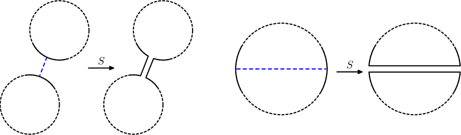
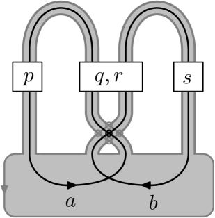
We say that two virtual knots and are concordant if can be transformed into by a finite sequence of births, deaths, saddle moves, and Reidemeister moves, such that . Births, deaths, and saddles are local moves on a virtual knot or link diagram; they are the same as in classical concordance. However, there is an equivalent description of them in terms of Gauss diagrams that is particularly convenient, and these are depicted in Figure 2. Thus a saddle is an oriented smoothing along a chord whose endpoints are disjoint from the endpoints of all other chords. A birth is the addition of a disjoint unknotted component, whereas a death is its removal. Saddles are indicated with a dotted line segment as in Figure 2.
Given an arbitrary virtual knot , it is elementary to show that there exists a finite sequence of births, deaths, and saddles transforming to the unknot. Given such a sequence, set , the genus of the surface cobordism from to the unknot, where are the numbers of births, deaths, and saddles, respectively. The slice genus of is defined to be the minimum over all such sequences. The virtual knot is said to be slice if it is concordant to the unknot, and it is called ribbon if it is concordant to the unknot by a sequence of moves that includes only saddles and deaths.
It is not known whether every slice virtual knot is ribbon. This is the virtual analogue of Fox’s question, which asks whether every classical slice knot is ribbon [Fox-1962-b]. Note that there could be classical knots which are virtually ribbon but not classically ribbon, i.e., knots which admit ribbon virtual knot diagrams but not ribbon classical knot diagrams. Thus, a weaker version of Fox’s question is whether every classical knot that is slice is virtually ribbon.
It is tempting to define concordance for welded knots in an analogous way. Recall that welded knots are equivalence classes of Gauss diagrams under the equivalence generated by Reidemeister moves along with the first forbidden move shown in Figure 3. However, concordance of welded knots leads a trivial theory, and in fact one can show that every welded knot is concordant to the unknot [Gaudreau-2018].

1.3. Concordance of knots in thickened surfaces
Given a Gauss diagram , we review the construction of the Carter surface . Our discussion is based on [Carter], and the analogous construction for virtual knot diagrams can be found in [Kamada-Kamada-2000].
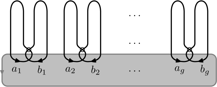
Suppose that has chords on the core circle O, which is oriented counterclockwise. The portions of O from one crossing to the next are called arcs. We thicken O to give an annulus and perform plumbings, one for each chord, according to its sign (see Figure 4). This results in an oriented surface with boundary, and we form a closed surface by gluing disks to each boundary component of the plumbed annulus. The resulting closed oriented surface is called the Carter surface.
Conversely, given a knot in a thickened surface , its crossing information determines a Gauss diagram which in turn determines a virtual knot. Stabilization of a knot in a thickened surface is the result of performing surgery on by attaching a 1-handle disjoint from . The opposite procedure is called destablization, and it involves surgery on removing a 1-handle disjoint from . Notice that stablization and destablization do not affect the underlying Gauss diagram, so they preserve the associated virtual knot. Two knots in and in in thickened surfaces are stably equivalent if they become equivalent under a finite number of stablizations and destablizations. By results of [Carter-Kamada-Saito], there is a one-to-one correspondence between virtual knots and knots in thickened surfaces up to stable equivalence.
In [Turaev-2008-a], Turaev studied concordance for knots in thickened surfaces, which is defined as follows.
Definition 1.1.
Two oriented knots in and in are called concordant if there exists an oriented -manifold with and an annulus with . If the annulus is smoothly embedded, then and are said to be smoothly concordant. If the annulus is locally flat, then and are said to be topologically concordant. A knot in which is (smoothly or topologically) concordant to the unknot is called (smoothly or topologically) slice.
One can verify that stably equivalent knots are smoothly concordant, and thus both notions of concordance of knots in surfaces induce equivalence relations on virtual knots. By [Carter-Kamada-Saito, Lemma 12], it follows that the notion of smooth concordance for virtual knots is equivalent to the definition in Subsection 1.2. See Figure 5 for an illustration of this correspondence.
1.4. Almost classical knots
In this subsection, we give three equivalent definitions of the index of a crossing in a virtual knot in terms of its three representations, namely as a virtual knot diagram, as a Gauss diagram, and as a knot diagram on a surface.
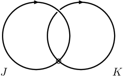
First, we review the definition of virtual linking numbers. Suppose is a virtual link with two components, and define as the sum of the writhe of the crossings where goes over . Notice that if is classical, then , but the virtual Hopf link in Figure 6 shows that this is not true in general for virtual links.
Suppose is a virtual knot diagram and is a crossing of . Then the oriented smoothing of at is a virtual link diagram with two components and , where denotes the component that contains the outward pointing over-crossing arc at . The index of is defined by setting
Now suppose is an arrow in a Gauss diagram , which we draw with pointing up. Set
where are the numbers of -arrows intersection and pointing to the right, and are the numbers of -arrows pointing to the left. An easy exercise shows that and thus this definition of agrees with the previous one.
Lastly, suppose is a knot in a thickened surface, and let denote the projection map. For any crossing of , let and be the two components obtained from the oriented smoothing at as above and set
| (1) |
the algebraic intersection of the homology classes .
Given a classical knot represented as a knot in , then the Jordan curve theorem implies that every chord of has The converse is however false, and virtual knots such that each chord has index zero are called almost classical [Silver-Williams-2006b].
Definition 1.2.
A virtual knot is almost classical if it can be represented by a Gauss diagram such that every chord satisfies .
One can alternatively define almost classical knots as those admitting Alexander numberable diagrams, and this approach generalizes to define almost classical links. As explained in [Boden-Gaudreau-Harper-2016], a virtual link is almost classical if and only if it can be represented by a homologically trivial link in a thickened surface. If is an almost classical knot or link, then by the modified Seifert algorithm in [Boden-Gaudreau-Harper-2016, §6], one can construct a compact oriented surface in with . We call a Seifert surface for .
2. Signatures for almost classical knots
In this section, we recall the Seifert pairing from [Boden-Gaudreau-Harper-2016] and use it to define invariants of almost classical knots. We extend the signature and Levine-Tristram signatures to almost classical knots, where unlike in the classical case, they depend on the choice of Seifert surface. Also, we introduce the directed Alexander polynomials of the pair , where is an almost classical knot and is a Seifert surface. These are two distinct generalizations of the Alexander-Conway polynomial. The main results are Theorems 2.5 and 2.8, which show that the Tristram-Levine signatures provide lower bounds on the slice genus and that the directed Alexander polynomials give slice obstructions.
2.1. Linking numbers
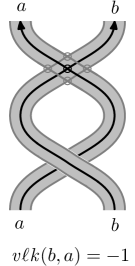
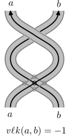
We review the basic properties of the linking numbers in . Let be disjoint oriented knots in . By [Boden-Gaudreau-Harper-2016, Proposition 7.1], we see that the relative homology group is infinite cyclic and generated by a meridian of . Let denote the homology class of in , and define to be the unique integer such that . The linking number can be computed as , the algebraic intersection number, where is a 2-chain in with for some 1-cycle in . In practice, to compute , we count, with sign, the number of times that crosses above in . Here, “above” is taken with respect to the positive -direction in . Thus, computing the linking number is formally similar to computing the virtual linking number, which were introduced in Subsection 1.4.
Linking numbers in are not symmetric but rather satisfy (see §10.2 [Cimasoni-Turaev]):
| (2) |
where is the algebraic intersection number in of the projections of and to .
2.2. Seifert forms and Seifert matrices
Suppose that is an almost classical link, realized as a homologically trivial link in . Suppose further that is a Seifert surface for . The Seifert forms are defined by , where denote the “pushoffs” of into . Each of and is bilinear, and they satisfy
| (3) |
where denotes the intersection form on the surface .
The Seifert forms are represented by a pair of Seifert matrices , which we introduce next. The homology group is a free abelian group of rank for some integer . Let be an ordered basis for , and define the two Seifert matrices by setting the entry of equal to . The Seifert matrices are not invariants of the almost classical link ; they depend on the choice of Seifert surface and basis for . A different choice of basis for alters the matrices by simultaneous unimodular congruence. Recall that an integral square matrix is said to be unimodular if it has determinant , and that two integral square matrices are said to be unimodular congruent if there is a unimodular matrix such that
Assume now that is almost classical knot with Seifert surface . For any pair of Seifert matrices , since the intersection form on is skew-symmetric and non-singular, equation (3) implies that is a skew-symmetric matrix satisfying In Subsection 3.2, we will see that any pair of integral matrices satisfying these conditions occurs as the Seifert matrices for some almost classical knot (cf. Theorem 3.7).
2.3. The Alexander-Conway polynomial
Suppose is an almost classical link, realized as a homologically trivial link in , and is a Seifert surface for . Let be the Seifert pair associated to , , and a choice of basis for The Alexander-Conway polynomial of is then defined by setting
A proof that is independent of the choice of Seifert surface and basis for can be found in [Boden-Gaudreau-Harper-2016], and it follows that is well-defined up to multiplication by , where is the virtual genus of , namely the smallest genus among all surfaces containing a representative for . In case is an almost classical knot, then .
For classical links, and this shows that is a balanced polynomial, i.e., that it satisfies Indeed, the Alexander polynomial of any classical knot satisfies: (i) and (ii) , where we write for if for some integer . A well-known result due to Seifert [Seifert-1935] shows that any integral polynomial of even degree satisfying (i) and (ii) occurs as the Alexander polynomial of a classical knot (see [Burde-Zieschang-Heusener, Theorem[8.13] for a proof).
If is an almost classical knot, it is no longer true that equals thus is not necessarily balanced. Nevertheless, the Alexander-Conway polynomial of any almost classical knot continues to satisfy the first condition. In Subsection 3.3 we will see that every integral polynomial with occurs as the Alexander polynomial of some almost classical knot (cf. Theorem 3.9).
2.4. Signature for almost classical knots
Suppose that is an almost classical link, realized as a link in , and that is a Seifert surface for in . The signature and nullity of the pair are defined to be
The following lemma implies that and , and henceforth we use and to denote the signature and nullity of .
Lemma 2.1.
.
Proof.
First note that for two knots on , . Let be a collection of simple closed curves on giving a basis for . Writing the Seifert matrices with respect to this basis, we see that has entry
The first term is the entry of the transposed matrix , thus it follows that , which proves the lemma. ∎
As in the classical case, it is useful to generalize the signature to Tristram-Levine signature functions, and in the case of an almost classical knot, we actually get a pair of signature functions. To define the signature functions, it is first necessary to define the directed Alexander polynomials, which are given by setting
Notice that , and they are balanced polynomials, namely they satisfy . We call the up Alexander polynomial and the down Alexander polynomial. Both polynomials depend on the choice of Seifert surface , and the up and down Alexander polynomials are generally distinct from one another and from the Alexander-Conway polynomial. Of course, for classical knots, all three polynomials coincide; i.e., if is classical then . In particular, in this case the up and down Alexander polynomials are independent of the choice of Seifert surface.
For a complex unit number, , the matrices are Hermitian, and we define the -signatures by setting
If the matrix is non-singular, then we will show that provides an obstruction to sliceness of . We will further relate non-singularity of the above Hermitian matrix to the vanishing of As usual, for we have that . Lemma 2.1 implies that , and notice also that
2.5. Signature and concordance of virtual knots
In this subsection, we study the signature functions and the directed Alexander polynomials as obstructions to sliceness. The method of the proof follows that of the classical case (cf. [Lickorish, Chapter 8]). The main issue is to adapt the classical proof to linking numbers in , as defined in §2.1.
The main results are Theorems 2.5 and 2.8, and they will follow from a sequence of lemmas, which we now state and prove.
For the next lemma, let be a knot in a thickened surface, a compact oriented -manifold with and a locally flat oriented surface in with . By [Freedman-Quinn, §9.3], has a normal bundle homeomorphic to , which we denote by .
Lemma 2.2.
The inclusion of pairs induces an isomorphism in homology .
Proof.
Let be inclusion, be projection onto the first factor, and be defined by . Note that . Since is an isomorphism, it follows that is a split surjection and is a split injection.
Let denote the interior of and apply a Mayer-Vietoris argument to to obtain
Since is split, the long exact sequence for the pair splits, giving the short exact sequence:
From the two short exact sequences, we conclude that is infinite cyclic. Since the summand of is generated by a meridian of , we conclude that the induced map sends a meridian of to a generator of . Thus the inclusion of pairs induces an isomorphism in homology as claimed. ∎
The next two results are adapted from Lemmas 8.13 and 8.14 in [Lickorish]. We provide detailed proofs for completeness.
Lemma 2.3.
For , suppose are maps of orientable surfaces into such that and that is a knot in . Then .
Proof.
Using standard arguments, it may be assumed each are locally flat embeddings. By definition, is the homology class of in . Since , is trivial in . Thus, . ∎
Lemma 2.4.
Let be a Seifert surface for in and let be a locally flat orientable surface in with . Then bounds a two-sided -manifold with .
Proof.
As above, let denote the normal bundle of in . We will construct a map of pairs
inducing an isomorphism on the relative first homology groups and so that is a 3-manifold with the desired properties. Throughout, we identify
Let be the complement of an open tubular neighborhood of in , and notice that In the following, we will identify with .
Define the map first on so that for , a product neighborhood of in , and so that maps the rest of to Notice that sends to and that is an isomorphism.
Now extend over the rest of so that , where is chosen so that is a longitude for .
In order to extend from to all of we use obstruction theory. We will work with an arbitrary but fixed triangulation of the pair . Let be a spanning tree in the 1-skeleton which includes a maximal tree in . Extend over so that it maps every 0-simplex and 1-simplex in to . For a 1-simplex not in define so that, for a 1-cycle obtained as the sum of and a 1-chain in , is the image of under the isomorphism of Lemma 2.2
To extend over the 2-simplices, note that the boundary of any 2-simplex is evidently trivial in Thus in , and can be extended over Similarly, can be extended over all 3-simplices, and then over all 4-simplices, such that is mapped to .
Choose a triangulation of in which 1 is not a vertex so that becomes a simplicial map of pairs, and notice that is a bi-collared 3-manifold in with boundary as claimed. ∎
The following theorem establishes the slice obstructions and slice genus bounds from the directed Alexander polynomials and the signature functions.
Theorem 2.5.
Let be an almost classical knot, represented as a knot in the thickened surface with Seifert surface , and suppose is an oriented -manifold with and is a locally flat orientable surface in with
If is a unit complex number such that , then Thus if is topologically slice, then , and in particular .
Proof.
Since it is always true that we can assume that . Let be the -manifold given by Lemma 2.4, so is compact and oriented and is a closed surface of genus , where is the genus of and is the genus of . By [Lickorish, Lemma 8.16], the subspace consisting of elements that map to zero under inclusion into has Thus has rank at least , and we can choose an integral basis of such that lie in and each is a simple closed curve on .
Let be the Seifert matrix . For , there are integers such that vanishes in . It follows that the curve bounds the image of an orientable surface mapped into . Pushing the into gives surfaces disjoint from each . Thus by Lemma 2.3, for This implies that there is a block of zeros in the upper left hand corner of .
In general, given a quadratic form over a field, a subspace consisting of elements for which is called isotropic, and the isotropy index of is the dimension of a maximal isotropic subspace. If is non-singular with rank and signature , then it is well-known that the isotropy index is given by where and , the number of positive and negative eigenvalues of .
Since and , the matrix:
is non-singular. Therefore, the quadratic form associated to the Hermitian matrix is also non-singular. Since the Seifert matrices both have a block of zeros, so does the Hermitian matrix. Thus the isotropy index of the quadratic form is at least Let be the signature of this quadratic form. Since it has rank , we see that Using this, one can easily show that and this completes the proof of the theorem. ∎
Example 2.6.
The almost classical knot has Seifert surface and basis for shown in Figure 7. By our convention, the positive push-offs and are obtained by pushing up along the lighter region of and down along the darker region. From this, one can readily compute that , and . Thus, the two Seifert matrices are given by
Therefore is a diagonal matrix with signature 2, and we see that . Theorem 2.5 applies to show that 4.105 is not slice. On the other hand, since 4.105 admits a genus one cobordism to the unknot, we see that its slice genus is equal to one.
The Alexander polynomial of a classical slice knot must satisfy the famous Fox-Milnor condition, which asserts that for some The following example shows that the Fox-Milnor condition fails for almost classical slice knots.
Example 2.7.
In Theorem 3.15, we will prove that any integral polynomial with occurs as the Alexander polynomial of an almost classical slice knot. Although the Fox-Milnor condition does not extend to almost classical knots using the Alexander polynomial, the following alternative formulation gives useful slice criteria in terms of the directed Alexander polynomials.
Theorem 2.8.
Let be an almost classical knot, represented as a knot in the thickened surface with Seifert surface . If is topologically slice, then there are polynomials such that .
Proof.
Let be a slice disk for . Repeating the previous argument with , it follows that there is a block of zeros in the upper left hand corner of the Seifert matrices . Thus, we can write these matrices in block form:
where are integral matrices.
Thus it follows that
Taking , the conclusion follows. ∎
Example 2.9.
For the almost classical knot with Seifert surface from the diagram in Figure 21, its Seifert pair is
The associated signature and -signatures all vanish, and so Theorem 2.5 is inconclusive on the question of whether this knot is slice.
On the other hand, the directed Alexander polynomials are given by
Neither of these polynomials satisfies the Fox-Milnor condition, so Theorem 2.8 implies that is not slice. In fact, applying a single crossing change to gives a slice knot, and thus it has slice genus one.
3. Realization theorems
In this section, we provide necessary and sufficient conditions for a pair of matrices to occur as the Seifert matrices of some almost classical knot, and we use it to show that any integral polynomial with occurs as the Alexander polynomial of some almost classical knot. The arguments are constructive and assume some familiarity with the basics of virtual knot theory as found, for example, in [Kauffman-1999, Kamada, Kauffman-2012]. We will also make essential use of virtual disk-band surfaces, which are prototypes of the more general notion of virtual Seifert surfaces defined and studied in [Chrisman-2017].
3.1. Virtual Disk-Band Surfaces
In this subsection, we introduce virtual disk-band surfaces, defined as follows.
Definition 3.1.
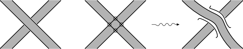
A virtual disk-band surface consists of a finite union of disjoint disks in , with a finite collection of bands in , connecting the disks. The bands may have (classical) twists, and in any region of the plane, at most two bands intersect. Each such band crossing is either classical or virtual as in Figure 8.
We will work exclusively with orientable virtual disk-band surfaces here, but we remark that Definition 3.1 can also be used to describe non-orientable spanning surfaces. Taking the boundary of a virtual disk-band surface gives a virtual knot diagram which is almost classical, and which can be seen as follows.
View the virtual disk-band surface in and construct a higher genus surface by attaching one-handles to at each virtual band crossing as in Figure 8. The 1-handles are attached to allow one band to pass along the 1-handle over the other band. The result is a disk-band surface in where has genus equal to the number of virtual band crossings of . The boundary of this disk-band surface is an almost classical knot in representing . The next lemma establishes the converse.
Lemma 3.2.
Suppose is an almost classical knot or link, realized as a knot or a link in a thickened surface . Then there exists a virtual disk-band surface whose boundary is a virtual knot diagram for .
Proof.
(sketch) The knot can be represented as a knot in with Seifert surface . Just as with any surface with boundary, can be decomposed as a union of disks and bands in . Assuming has genus , it can be realized as the identification space of the -gon , drawn in the plane, under the usual identification of its sides. Under further isotopy, we can arrange that the images of the disks of are pairwise disjoint and lie in the interior of , and that the images of the bands are disjoint from the disks and that at most two bands meet in any region. We can also arrange that the bands meet the boundary of the -gon only along its edges and not at any of its vertices. It is now a simple matter to draw the associated virtual disk-band surface in the plane by extending the bands of outside the -gon and introducing virtual crossings whenever two bands cross outside . The result is a virtual disk-band surface with boundary a virtual knot diagram for ∎
Figure 9 shows the evolution of a Seifert surface in to a virtual disk-band surface for the almost classical knot 6.90228. An orientation of induces an orientation on the Seifert surface and the virtual disk-band surface , and this determines the directions of the positive and negative push-offs. Here we follow the convention used in Subsection 4.1, so a small left-handed meridian pierces and from the negative side and exits from the positive side. For example, in Figure 9, over the shaded regions of and , the positive push-off is above the page, and elsewhere it is below the page.
The next lemma follows from a straightforward comparison between the conventions for computing linking numbers of curves in relative to and the conventions for computing virtual linking numbers. The details are left to the reader.
Lemma 3.3.
Suppose is an almost classical knot, realized as a knot in a thickened surface with Seifert surface . Suppose are simple closed curves giving a basis for , and let be their images on the virtual disk-band surface associated to as in Lemma 3.2. Then
| (4) |
As a consequence of Lemma 3.3, the Seifert matrices associated to an almost classical knot with Seifert surface and a choice of basis for can be computed entirely in terms of the virtual linking numbers of the corresponding curves on the virtual disk-band surface associated to as in Lemma 3.2.
Example 3.4.
Consider the virtual disk-band surfaces shown in Figure 9. Using the basis in the last frame, one can compute the Seifert pair associated to this surface to be
Just as in the classical case, the calculation of the Seifert matrices is especially simple when the virtual disk-band surface consists of only one disk with bands attached, and this can always be arranged by isotopy. In that case, the cores of the bands are simple closed curves on which give a natural choice of basis for , and each band has an even number of half twists, and as such can be drawn without twists by using positive or negative kinks (cf. Figure 11). Virtual disk-band surfaces of that form are called virtual band surfaces and they are especially useful in establishing the realization theorems for Seifert pairs in the next two subsections.
3.2. Realization of Seifert pairs
In Subsection 2.2, we observed that any pair of Seifert matrices for an almost classical knot satisfies is skew-symmetric and In this subsection, we establish the converse result. We begin with the following definition.
Definition 3.5.
A Seifert pair is a pair of integral square matrices such that is skew-symmetric and Equivalence of Seifert pairs is given by simultaneous unimodular congruence.
Remark 3.6.
If is a Seifert pair, then a standard argument (see [Burde-Zieschang-Heusener, A1], for instance) shows that is unimodular congruent to , a block sum of copies of the matrix:
| (5) |
The next theorem is the main result in this section, and we will prove it by constructing a virtual band surface realizing any given Seifert pair .
Theorem 3.7.
A pair of integral square matrices represents the pair of Seifert forms associated to an almost classical knot with Seifert surface if and only if is skew-symmetric and
Proof.
Suppose is a Seifert pair (cf. Definition 3.5). Our goal is to construct an almost classical knot and Seifert surface whose Seifert matrices equal . Notice that it is enough to prove this up to simultaneous unimodular congruence, because if a Seifert pair is realized by some almost classical knot and Seifert surface and choice of basis for , then any pair of matrices simultaneously unimodular congruent to can be realized by making a change of basis for .
Suppose then that is a pair of integral square matrices such that is skew-symmetric and By Remark 3.6, we have that is unimodular congruent to the block sum . Therefore, it is sufficient to prove the statement under the assumption that . In this case, is determined by , thus we will show that any integral square matrix can be realized as the Seifert matrix of a virtual band surface.
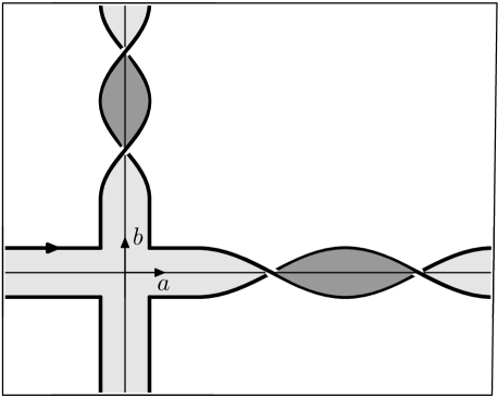
The proof is by induction on . For , consider the virtual band surface given in Figure 10. Here denotes an ordered basis for , as discussed in Section 3.1, and an easy exercise shows that the intersection form is represented by the matrix with respect to this basis. The labelled boxes in Figure 10 indicate the number and types of kinks and virtual half twists that need to be inserted.

For instance, suppose
Then to realize as the virtual linking matrix, insert kinks on the first band and kinks on the second, using right handed kinks when or is positive and left-handed kinks when they are negative (see two kinks on left in Figure 11). Also insert virtual half twists where crosses over and virtual half twists where crosses over , again using right-handed virtual twists when or is positive and left-handed virtual twists when or is negative (see four virtual half twists on right of Figure 11). With these choices, it is not difficult to verify that
Thus, this virtual band surface has Seifert matrix with respect to the basis
To proceed with the proof, we argue by induction. Suppose is a pair of integral square matrices such that is skew-symmetric and Under simultaneous unimodular congruence, we can arrange that . As before, it is enough to construct a virtual band surface realizing . Write , where , and set and . Thus, and are the diagonal block submatrices of of sizes and , respectively, such that:
By induction, we have virtual band surfaces realizing and , and Figure 12 depicts a virtual band surface obtained from combining these two surfaces. In the figure, bands are represented by lines. The large boxes labelled and indicate what can be arranged by induction. Furthermore, it is straightforward to see that, with the indicated basis for , the intersection form is a block sum of copies of the matrix . Thus .
To complete the proof, one must insert virtual twists into the small unlabelled boxes in Figure 12, and these are chosen to achieve the desired linking of the last two bands around the first bands. This will involve a combination of left or right virtual half twists, as shown in Figure 11, and here we no longer assume is oriented upwards. To be very specific, for the box involving the bands and , where and , we insert the 2-strand virtual braid so that and . The pair of Seifert matrices for the resulting virtual band surface with respect to the basis is now equal to the given matrices and this completes the induction and finishes the argument. ∎
3.3. Realization of Alexander polynomials
For any almost classical knot, the Alexander polynomial satisfies , and in this subsection, we establish the converse result, that any integral polynomial satisfying occurs as the Alexander polynomial of some almost classical knot.
The proof uses Theorem 3.7, and we begin by defining the algebraic Alexander polynomial associated to an integral square matrix defined as
Setting , we see that this polynomial satisfies . The following lemma is useful and proved using companion matrices. The details are left to the reader.
Lemma 3.8.
For any integral polynomial satisfying , there exists an integral square matrix with
Theorem 3.9.
For any integral polynomial satisfying , there exists an almost classical knot with
Proof.
Let be the block sum of copies of the matrix from equation (5). Thus, is an integral square matrix with and where denotes the identity matrix.
Suppose is an integral square matrix. By Theorem 3.7, we can find an almost classical knot whose Seifert matrices satisfy and
Therefore,
Thus, there exists an almost classical knot with . Lemma 3.8 implies that any integral polynomial satisfying can be realized as for some integral square matrix , and the above argument shows the same is true for the Alexander polynomials of almost classical knots. This completes the proof. ∎
Remark 3.10.
In fact, in Theorem 3.15 we will see that any integral polynomial with can be realized as the Alexander polynomial of a slice and even ribbon almost classical knot.
3.4. Realization for null-concordant Seifert pairs
The notion of algebraic concordance for almost classical knots is defined in terms of null-concordant Seifert pairs, which we introduce next.
Definition 3.11.
A pair of integral square matrices is called null-concordant if and are simultaneously unimodular congruent to matrices in block form:
where are integral matrices.
The proof of Theorem 2.8 shows that, if is an almost classical slice knot and is any Seifert surface for , then the associated Seifert pair is null-concordant. More generally, if is any almost classical knot with Seifert surface such that the Seifert pair is null-concordant, then Theorems 2.5 and 2.8 continue to hold. This is summarized in the following proposition.
Proposition 3.12.
Suppose is an almost classical knot with Seifert surface such that the associated Seifert pair is null-concordant. Then for any unit complex number such that we have Further, there exist polynomials such that .
The next theorem shows that every null-concordant Seifert pair can be realized by an almost classical knot which is slice.
Theorem 3.13.
Suppose is a pair of integral square matrices such that is skew-symmetric and . Then is null-concordant if and only it occurs as the Seifert pair of an almost classical knot which is slice.
Proof.
Suppose is the Seifert pair associated to an almost classical knot with Seifert surface . If is slice, then as in the proof of Theorem 2.8, it follows that is null-concordant. This proves the theorem in one direction.
To prove the converse, suppose is a null-concordant pair of integral square matrices with skew-symmetric and . We will construct an almost classical knot which is slice and admitting as a Seifert pair. In fact, it will follow from the construction that is actually ribbon.
Since is skew-symmetric and unimodular, the bilinear form on the free module defined by for is a non-degenerate skew form. For a submodule , we define
A submodule is called isotropic if , and a basis for is said to be symplectic if and for all
We claim that there is a symplectic basis for such that the restrictions of and to the submodule generated by are both trivial.
The claim is proved by induction on . For , null-concordance implies there is a basis such that and both vanish on Then is isotropic for . Further, since replacing with if necessary, we can arrange that is a symplectic basis for .
Now suppose it has been proved for free abelian groups of rank and consider Null-concordance implies there is a primitive submodule of rank on which and vanish. Clearly is isotropic, in fact one can easily see that Let be a basis for and be the submodule generated by Then and the basis can be extended to a basis for by adding one element , which can be chosen so that (since is unimodular). Notice that restricts to a non-degenerate form on the submodule generated by Set Then restricts to a non-degenerate skew form on , which has rank , and is isotropic with respect to the restriction, and we apply induction.
Since it is enough to prove the theorem up to simultaneous unimodular congruence, by the claim we can arrange that
| (6) |
For such pairs, is determined by . The proof of Theorem 3.7 given in Subsection 3.4 already shows how to construct a virtual band surface with prescribed Seifert matrix , and we will explain how the assumption of null-concordance results in this surface bounding an almost classical knot that is slice. As a warm-up, we give the proof in case .
For instance, suppose
and . Clearly the Seifert pair is null-concordant, and the virtual band surface depicted in Figure 10 with realizes the Seifert pair .
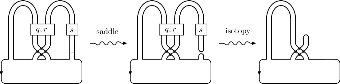
We claim that the almost classical knot bounded by this surface is slice, and the movie in Figure 13 gives the concordance to the unknot. In fact, after performing one saddle at the base of the second band on the right, the resulting link is isotopic by a sequence of Reidemeister II move and virtual Reidemeister II moves to the trivial link with two components. Performing one death results in the unknot, and this produces a ribbon concordance to the unknot. This shows that the original knot is ribbon and completes the proof in the case .
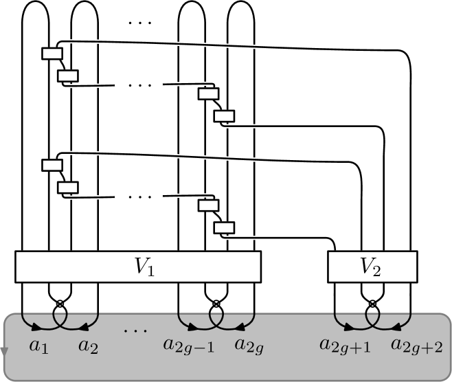
A virtual band surface can be constructed realizing any such null-concordant pair as in the proof of Theorem 3.7. Here, we label the bands according to Figure 14, where bands are drawn as lines. It depicts the virtual band surface with bands whose boundary is the trivial knot. We can modify this surface to realize any Seifert pair satisfying (6) by only altering the second set of bands but leaving the first set of bands trivial. Redrawing the second set of bands to allow them to virtually link themselves and the first set of bands arbitrarily, and adding kinks to the second set of bands as needed, we can realize any null-concordant Seifert pair satisfying (6).
It remains to show the resulting virtual knot bounding this surface is slice, and the following lemma is useful.
Lemma 3.14.
Performing saddle moves to each of bands and applying the lemma, we obtain a component virtual unlink. This describes a ribbon concordance to the unknot, and it completes the proof of the theorem. ∎
We close this section with the next result, which is in marked contrast to the situation for classical knots.
Theorem 3.15.
For any integral polynomial satisfying , there exists a ribbon almost classical knot with
Proof.
Since , we can write for some with . Let
where is the identity matrix. Consider the matrices of size written in block form:
Here, is an arbitrary integral matrix, and
is the companion matrix to .
Obviously, , and the Seifert pair is evidently null-concordant. By Theorem 3.13, there is an almost classical knot which is ribbon and which realizes the pair . Furthermore, this knot has Alexander polynomial
∎
4. Applications
In this section, we apply Theorems 2.5 and 2.8 to the problem of determining the slice genus for every almost classical knot up to six crossings, and this step relies on computations of the Seifert matrices (see Table 3) and Turaev’s graded genus (see [Boden-Chrisman-Gaudreau-2017, Boden-Chrisman-Gaudreau-2017t]). We show that the directed Alexander polynomials satisfy a skein relation and study how the knot signature behaves under crossing changes.
4.1. Computations
In this subection, we explain how to compute the Seifert matrices and signatures for almost classical knots. To start off, we take a homologically trivial knot in a thickened surface and apply Seifert’s algorithm to construct a Seifert surface. This method was used to produce the Seifert matrices for almost classical knots with up to 6 crossings in Table 3, namely we applied Seifert’s algorithm to the knots in surfaces depicted in Figure 21 and computed linking pairings.
In all computations, the top of the Carter surface is facing up, and the orientation of the Seifert surface determines the direction of the positive and negative push-offs. We follow the conventions of [Boden-Gaudreau-Harper-2016] in this aspect, which means that we parameterize a regular neighborhood of the Seifert surface as such that a small oriented meridian of enters at and exits at Our convention is that meridians are left-handed.
It is helpful to notice that the oriented smoothing of a knot in a thickened surface depends only on the underlying flat knot, which is the virtual knot up to crossing changes, and so we organize the almost classical knots into families according to their underlying flat knot. Notice further that the Seifert surfaces of two knots with the same underlying flat knot differ only in the types of half-twisted bands that are attached. For positive crossings, the attached band has a left-handed twist, and for negative crossings, the band has a right-handed twist.
Example 4.1.
Consider the almost classical knots 5.2012, 5.2025, 5.2133, and 5.2433, which all have the same underlying flat knot. Each occurs as a knot in a Carter surface of genus two and admits a Seifert surface of genus two. Two of the knots in this family are slice (5.2025 and 5.2133), and we will mainly focus on the other two.
In this family of 5-crossing almost classical knots, 5.2012 is obtained by performing a crossing change to 5.2433, and each of 5.2025 and 5.2133 are obtained by a crossing change to 5.2012. Since all the knots in the family are related by crossing changes, one can use Conway’s method to perform some of these computations. We will return to this in Example 4.2 below.
Consider the Seifert surfaces in Figure 15 for 5.2012 and 5.2433. Also depicted there is a basis of simple closed curves for . The shaded part of is the positive side and the unshaded part is the negative side. Thus the positive push-offs of lie above along the shaded portion and below it along the unshaded portion. Recall further that if are two simple closed curves in that do not intersect, then is an algebraic count of only the crossings when goes over (this is because linking is taken in the relative homology of the pair
For 5.2433, one obtains that
Thus and The directed Alexander polynomials are equal in this case and given by . This polynomial has roots at the fifth roots of , and takes values .
For 5.2012, one obtains that
Thus and The directed Alexander polynomials are again equal and given by . This polynomial has roots at the third roots of , and takes values .
It should be noted that the Seifert matrices in Table 3 are computed with just one choice of Seifert surface, and different choices would lead to possibly different signatures, -signatures, and directed Alexander polynomials. Passing to a second Seifert surface is useful in finding slice obstructions for a given almost classical knot, and we apply this method to show 5.2439, 6.72695, 6.77908, and 6.87548 are not slice in Subsection 4.3.
4.2. Conway’s method
Conway developed methods for computing the Alexander polynomial and signatures of classical knots using crossing changes, and these methods carry over to give skein formulas for the directed Alexander polynomials and the signature of almost classical knots. (The Alexander polynomial of almost classical knots also satisfies a skein relation, see [Boden-Gaudreau-Harper-2016, Theorem 7.11] for more details.) We begin by reviewing the situation for classical knots.
Suppose and are classical knots that are identical except at one crossing, which is positive for and negative for . Choosing Seifert surfaces for and that differ only in the half-twisted band at the crossing, and choose a basis for its first homology so the first generator passes through the crossing and all the other generators do not. It follows that the Seifert matrices and are the same except for the entry, in fact, we have
where is the self-linking of the first generator, and are row and column vectors, respectively, and represents the Seifert matrix for the two component link obtained from the -smoothing of . Arguing as in [Giller-1982], it follows that the Alexander polynomials satisfy the skein relation
and the knot signatures of and differ by at most two. In fact, one can further show that
| (7) |
so either or .
In general, for any non-singular symmetric real matrix, its signature modulo 4 is determined by the sign of its determinant. Applying this observation to the symmetrized Seifert matrix of a knot , since it is a matrix with , it follows that
| (8) |
Thus one can determine from entirely by comparing the signs of and ; if the signs are the same then , otherwise
Similar formulas hold for almost classical knots provided one uses compatible Seifert surfaces for and , which will be denoted and , respectively and which are assumed to be identical except for the half-twisted bands at the crossing. One must further assume that the symmetrized Seifert matrices for , and are all non-singular, which is automatic for classical knots but which does not always hold for almost classical knots. Under those assumptions, for appropriate choices of generators, the Seifert matrices and are given by
It follows that the directed Alexander polynomials satisfy the skein relation
| (9) |
and that equations (7) and (8) continue to hold, where in the second formula is replaced by (Notice that Lemma 2.1 implies that )
Example 4.2.
In this example, we apply Conway’s method to determine the effect on the signature of the crossing change for the virtual knots 5.2012 and 5.2433 depicted in Figure 15. Note that 5.2433 has all negative crossings, and that 5.2012 is obtained by changing one of the crossings of 5.2433.
4.3. Slice obstructions
In this subsection, we apply the previous results to the question of sliceness of almost classical knots. Combined with the graded genus [Boden-Chrisman-Gaudreau-2017, Boden-Chrisman-Gaudreau-2017t], the computations are sufficient to determine sliceness for all almost classical knots up to six crossings. These results are presented in Table 2 at the end of the paper, which gives the graded genus, signature, and -signatures for these knots. The almost classical knots that are known to be slice are also displayed with their slicings in Figure 20.
All the other knots in the table can be seen to be non-slice, and we explain this now. In the majority of cases, this follows by applying Theorem 2.5, using either the signature or -signatures. When the signatures and -signatures fail to obstruct sliceness, we apply Theorem 2.8 or the graded genus. For instance, the knots and are classical, and although their signatures and -signatures all vanish, their Alexander-Conway polynomials, which are and do not factor as , and so Theorem 2.8 applies to show that neither nor is slice.
In a similar way, one can use the directed Alexander polynomials to obstruct sliceness for the knots 6.87857 and 6.90194. For , the directed Alexander polynomials are and , neither of which factors as , so Theorem 2.8 applies to show it is not slice. Likewise, has down polynomial which does not factor so is not slice.
The five almost classical knots 6.77905, 6.77985, 6.78358, 6.85091, and 6.90232 all have graded genus . Since is a concordance invariant of virtual knots [Boden-Chrisman-Gaudreau-2017], it follows that none of them are slice.
In some cases, we obstruct sliceness using invariants derived from a second Seifert surface . The new surface is obtained from the standard one by connecting it to a parallel copy of the Carter surface by a small tube. For instance, for , the new Seifert matrices are
From this, it follows that , and Theorem 2.5 applies to show is not slice. For , using a second Seifert surface , we find that takes values , and Theorem 2.5 again shows it is not slice.
4.4. Slice genera
In this subsection, we return to the question [Dye-Kaestner-Kauffman-2014] mentioned in the introduction on the virtual slice genus of classical knots, which we rephrase optimistically below as a conjecture. We begin with a brief review of the slice genus for virtual knots.
The (smooth) slice genus of a virtual knot was introduced in Subsection 1.2 and is related to the virtual unknotting number of (see [Boden-Chrisman-Gaudreau-2017]). Computations of the slice genus for many virtual knots with up to six crossings are given in [Boden-Chrisman-Gaudreau-2017, Rushworth-2017], and a table of these computations can be found online [Boden-Chrisman-Gaudreau-2017t].
The topological slice genus is defined as the minimum genus over all topological locally flat embedded oriented surfaces in with , where is a 3-manifold with and is a representative knot in (cf. Definition 1.1). The following conjecture was posed as an open problem by Dye, Kaestner, and Kauffman [Dye-Kaestner-Kauffman-2014].
Conjecture 4.3.
For any classical knot, its smooth and topological slice genus as a virtual knot agree with its smooth and topological slice genus as a classical knot.
Using and to denote the smooth and topological slice genera as a classical knot, the conjecture asserts that, if is classical, then
| (10) |
Using KnotInfo [Knotinfo], one can use the signatures and Rasmussen invariants to verify this conjecture for classical knots with up to 12 crossings. This step implicitly uses the fact that the signatures and Rasmussen invariant extend to the virtual setting. The first is proved here, and the second is a consequence of [Dye-Kaestner-Kauffman-2014].
The next result provides a summary of our findings.
Proposition 4.4.
For classical knots with up to 10 crossings, Conjecture 10 is true for both the smooth and topological slice genera.
For classical knots with 11 crossings, Conjecture 10 on the topological slice genus is true in all cases. The conjecture on the smooth slice genus is true with just two possible exceptions: and
Proof.
The main result in [Boden-Nagel-2016], which holds for both smooth and topological concordance, implies that equation (10) holds for any classical knot with smooth slice genus equal to one. Thus, to confirm the conjecture, we only need to consider knots with .
For classical knots with up to ten crossings, for all but five cases, either or . This confirms the conjecture in all cases except for the knots:
Interestingly, each one has and satisfies and Combining our signature results with the results of [Dye-Kaestner-Kauffman-2014] on Rasmussen’s invariant, it follows that (10) holds for these five knots. We conclude that Conjecture 10 holds for all knots with up to 10 crossings.
In a similar way, one can check the conjecture on all the classical knots with 11 crossings, and it can be confirmed for all but the following six knots, namely
The smooth slice genus is unknown for and the other five have Four of them satisfy and , so (10) holds for these four. This confirms the conjecture for classical knots with 11 crossings with two possible exceptions: and
Similar methods apply to 12 crossing knots. For example, the topological slice genus has been computed for all 12-crossing knots except for the following seven [Lewark-McCoy-2017], [Knotinfo]:
| (11) |
For the other knots with 12-crossings, one can check that they all satisfy or , except for the following eight [Knotinfo]:
| (12) |
This confirms that for classical knots with 12 crossings with 15 possible exceptions.
The smooth slice genus has been computed for all 12-crossing knots except for the following 20 [Lewark-McCoy-2017], [Knotinfo]:
| (13) |
For the other knots with 12-crossings, one can check that they all satisfy or , except for the following 17 [Knotinfo]:
| (14) |
This confirms that for classical knots with 12 crossings with 37 possible exceptions. ∎
For almost classical knots up to six crossings, our methods were not able to determine the slice genus in four cases:
For the first three, the signature tells us that , and for 6.90194, Theorem 2.8 implies that . Further, by the results of [Boden-Chrisman-Gaudreau-2017], we know that for all four. In the classical case, for stubborn knots such as with vanishing signature, signature function, and Rasmussen invariant, the slice genus can be investigated by other techniques, such as the -genus and the triple point method [Murakami-Sugishita-1984]. It would be interesting to generalize these results to virtual knots, and in their recent paper [Fedoseev-Manturov-2017], Fedoseev and Manturov define a slice criterion for free knots using triple points of free knot cobordisms. Their work represents a promising development toward realizing this goal.
At the end of this paper, we have included a number of figures and tables of almost classical knots with up to six crossings. Figure 20 shows all the slice almost classical knots, with the slicing indicated as a saddle move on the Gauss diagram. Table 1 gives their Alexander-Conway polynomials and Table 2 shows their graded genus, signature, -signatures, and slice genus. Figure 21 gives realizations of each almost classical knot as a knot in a thickened surface. The knot diagrams determine Seifert surfaces in the usual way, and the resulting pairs of Seifert matrices are listed in Table 3. Note that the Tables 1, 2, and 3 include classical knots.
5. Parity, projection, and concordance
In this section, we introduce Manturov’s notion of parity projection and Turaev’s construction of lifting of knots in surfaces. The main result is that parity projection preserves concordance, and it is established by interpreting parity projection in terms of lifting knots to coverings.
5.1. Parity and projection
A parity is a collection of functions , one for each Gauss diagram in the diagram category, which is a category whose objects are Gauss diagrams and whose morphisms are compositions of Reidemeister moves. Given , the function is a map from the chords of to the set Chords with are called odd, and those with are called even. The collection of functions is required to satisfy the following:
Parity axioms
Suppose and are related by a single Reidemeister move.
-
(0)
The parity of every chord not participating in the Reidemeister move does not change.
-
(1)
If and are related by a Reidemeister I move which eliminates the chord of , then, .
-
(2)
If and are related by a Reidemeister II move which eliminates the chords and of , then, .
-
(3)
If and are related by a Reidemeister III move, then the parities of the three chords involved in the Reidemeister III move do not change. Moreover, the three parities involved in the move are either all even, all odd, or exactly two are odd.
In [Manturov-2010], this is referred to as “parity in the weak sense”. Readers interested in more details on parity are referred to [Manturov-2010], [Ilyutko-Manturov-Nikonov-2011] and [Nikonov-2016].
Given a parity , there is a map on Gauss diagrams called parity projection and denoted . For a Gauss diagram , its image under parity projection is the Gauss diagram obtained from by eliminating all of its odd chords.
Proposition 5.1 ([Manturov-2010]).
If and are two Gauss diagrams equivalent through Reidemeister moves, then their parity projections and are also equivalent through Reidemeister moves.
This result is a direct consequence of the parity axioms. Although parity projection is defined in terms of the underlying Gauss diagram, Proposition 5.1 implies that it is well-defined as a map on virtual knots.
Since each application of parity projection removes chords from the Gauss diagram , we have for sufficiently large. Using this observation, we define , and we call the stable projection with respect to the parity . Although stable projection is defined on the level of the Gauss diagrams, it gives rise to a well-defined map on virtual knots.
5.2. Gaussian parity
We now consider Gaussian parities, which are defined in terms of the indices of the chords in a Gauss diagram.
Definition 5.2.
Let be an integer and a Gauss diagram. The mod Gaussian parity is defined by setting, for any chord of ,
Here, we denote mod Gaussian parity by , its associated parity projection by , and stable projection with respect to by . For example, the mod parity projection acts on a Gauss diagram by removing all chords whose index is nonzero modulo , and the image of consists of all Gauss diagrams with for every chord of . A virtual knot satisfies this condition if and only if it can be represented as a knot in a thickened surface which is homologically trivial in (see §5 of [Boden-Gaudreau-Harper-2016]).
Another very useful parity is the total Gaussian parity, which is defined next.
Definition 5.3.
The total Gaussian parity is defined by setting, for any chord of ,
Alternatively, if is a Gauss diagram, one can define the total Gaussian parity by setting . Indeed, taking to be larger than the number of chords of , one can easily see that if and only if
Throughout this paper, we denote total Gaussian parity by , its associated parity projection by , and the stable projection with respect to by For example, the parity projection acts on a Gauss diagram by removing all chords whose index is nonzero, and the image of consists of Gauss diagrams with for every chord of , i.e., almost classical knots.
5.3. Coverings and Parity
In this subsection, we show how to interpret Gaussian parity projection of a virtual knot represented as a knot in a thickened surface in terms of Turaev’s lifting along an abelian covering of the surface [Turaev-2008-a]. Using this approach, we prove that if two virtual knots and are concordant, then their images and under parity projection are concordant (see Theorems 5.9 and 5.11).
In general, if is a covering of surfaces and is a knot in then Turaev observed that one can lift by taking to be the knot in given as a connected component of the preimage . The equivalence class of can be shown to be independent of the choice of connected component, and one can define invariants of in terms of invariants of the lifted knot .
We review this construction and relate the knots obtained by lifting along abelian covers to those obtained by projection with respect to Gaussian parity. This correspondence gives a natural topological interpretation of parity projections, and we use it to prove that parity projection preserves concordance. We begin with Turaev’s construction for lifting knots along covers and explain how it is related to parity projection.
Let be a closed oriented surface, the projection, and a knot in . Fix an integer and consider the homology class . Its Poincaré dual determines an element in , and precomposing with the Hurewicz map, we obtain a homomorphism . The proof of the next result is standard and left to the reader.
Lemma 5.4.
For , .
The kernel of yields a regular covering space of finite index. Moreover, the map sends the homotopy class of to . Hence, lifts to a knot in . As any lift of may be obtained from any other lift by a diffeomorphism of , all lifts of represent the same virtual knot. The knot is called a lift of .
Example 5.5.
If the map is trivial, then and . If the group of covering transformations of is non-trivial and at each crossing point of the over-crossing arc and under-crossing arc lift to different sheets, then is a simple closed curve on representing the trivial virtual knot.
The next lemma relates the lift of a virtual knot to its image under mod parity projection.
Lemma 5.6.
Let be a knot in and the lift of to the covering space . Then the Gauss diagram of is obtained from the Gauss diagram of by deleting the chords with . In particular, as virtual knots, the lift of is equivalent to its image under parity projection.
Proof.
Let be a double point of , where . Applying the oriented smoothing at gives knots and on , and using equation (1) and the fact that holds for any , we see that
Now viewing as an element of , the lifting criterion and Lemma 5.4 imply that lifts to a closed curve in the covering space precisely when . On the other hand, if is a crossing with , then does not lift to a closed curve in the covering space , hence this crossing does not appear in the lifted knot . Thus the Gauss diagram of is obtained from by deleting those chords with . ∎
Example 5.7.
Starting with the Gauss diagram on the left of Figure 16, we find a representative knot in a surface. Its depiction is not unique, as the surface can be stabilized, and Dehn twists can be applied, which alter the homology class represented by the knot diagram. For , two such representatives are depicted on the right of Figure 16. They are inequivalent as knots in thickened surfaces, but have the same underlying Gauss diagram. Let be the knot in the 2-torus depicted on the left in Figure 16, and let be the generators for its first homology. Notice that , hence, the lift of to the 2-fold cover is obtained by gluing two copies of along and identifying the remaining opposite sides. The lifted knot is depicted in Figure 17, and one can check that the Gauss diagram for the lift is obtained by forgetting the grey arrows of .
The following lemma, due to Turaev, shows how concordance behaves under lifting knots along coverings.
Lemma 5.8 (Lemma 2.1.1, [Turaev-2008-a]).
Suppose is a knot in the thickened surface for . If and are concordant, then the lifted knots and are also concordant.
The following is the main result in this section, and it implies that parity projection preserves concordance.
Theorem 5.9.
Suppose is a virtual knot for and is an integer with If is concordant to , then their images and under parity projection are concordant.
Proof.
Example 5.10.
Consider the virtual knot , whose Gauss diagram appears on the left in Figure 18. In [Boden-Chrisman-Gaudreau-2017t], we show that it has virtual slice genus Applying parity projection with respect to total Gaussian parity, the resulting knot has Gauss diagram on the right in Figure 18. We see that is the reverse of 4.107, and in [Boden-Chrisman-Gaudreau-2017] we show that 4.107 has graded genus It follows that is not slice, and Theorem 5.9 implies that is also not slice. Hence


The next result follows by repeated application of Theorem 5.9.
Theorem 5.11.
If and are virtual knots and is concordant to , then their images and under stable projection are concordant for any and
In particular, taking in Theorem 5.11 allows us to reduce questions about concordance of virtual knots to questions about concordance of almost classical knots. In terms of the Tristram-Levine signatures defined for almost classical knots in Section 2, Theorem 5.11 shows that they lift to define slice obstructions for all virtual knots.
We give an application of Theorem 5.9 to show that the polynomial invariants introduced in [Jeong-2016] and [Im-Kim-2017] are concordance invariants of virtual knots.
In [Jeong-2016], Jeong introduced the zero polynomial , and in [Im-Kim-2017], Im and Kim give a sequence of polynomial invariants for a non-negative integer. They note that for and they give a formula for computing in terms of Gauss diagrams (see Definition 3.1 of [Im-Kim-2017]).
It is clear from that formula that is equal to the index polynomial applied to , where denotes mod Gaussian parity projection. Theorem 7 of [Boden-Chrisman-Gaudreau-2017] shows that the writhe polynomial and Heinrich-Turaev polynomial are concordance invariants. The following, which concerns the polynomials invariants and introduced in [Im-Kim-2017] and [Jeong-2016], respectively, is an immediate consequence of combining the above observations with Theorem 5.9.
Corollary 5.12.
The polynomials of Im and Kim are concordance invariants for virtual knots. In particular, the zero polynomial of Jeong is a concordance invariant for virtual knots.
Theorem 5.9 says that the projection with respect to Gaussian parity preserves concordance, and it is an interesting question to determine which other parities have the property that projection preserves concordance.
5.4. Iterated lifts of knots
In this subsection, we present analogues of Lemma 5.6 and Theorem 5.9 for iterated lifts and iterated projections. Given a knot in the thickened surface and a finite sequence of integers , with for , the iterated lift of is the knot
in the thickening of the iterated covering space
The next result is obtained by repeated application of Lemma 5.6 and Theorem 5.9.
Proposition 5.13.
Suppose are integers with for .
-
(i)
As virtual knots, the iterated lift of is equivalent to the image under iterated application of parity projection.
-
(ii)
If and are virtual knots and is concordant to , then their images and under iterated projections are concordant.
Proposition 5.13 raises the question of commutativity of iterated projections, and the simplest instance is whether , or equivalently whether More generally, one can ask whether the iterated lifts are independent of the order . To that end, let denote the normal subgroup of defining the covering space . The relationship between the lifts of is entirely determined by the structure of the lattice of normal subgroups of . Thus, the question of commutativity of iterated lifts is really a question about the structure of the lattice of normal subgroups.
Consider, for example, the portion of the lattice of regular covering spaces in the commutative diagram below. Here are integers, and is any non-zero multiple of . The expression on each arrow corresponds to the index of the covering projection. For simplicity of exposition, we will assume that the indices of the covering maps are as indicated, although this need not be the case in general. Note that since and there are natural maps and . It follows from the definition of that . Hence, and are also covering projections.
Furthermore, the homotopy class of is an element of each of , , and . Since the diagram commutes, it follows from the lifting criterion that is a lift of both and . The following theorem shows how to obtain the Gauss diagram of from that of either or . In this instance, it follows that
Theorem 5.14.
The Gauss diagram of is obtained from the Gauss diagram of by deleting the chords whose index in are and . Similarly, is obtained from the Gauss diagram of .
Proof.
The Gauss diagram is obtained from by deleting those chords having index , and is obtained from by deleting those chords that have index . Since , the only chords of that need to be deleted from to obtain are those having index and . ∎
On the other hand, by Lemma 5.6, the Gauss diagram can be obtained from by deleting chords in with index . We may similarly obtain from . In the general case, it is not always true that , and in certain cases, it may turn out that the iterated covering is nonabelian, as explained in the next proposition.
Proposition 5.15.
The group of covering transformations of is a group extension of by . In other words, there is short exact sequence
Proof.
This follows immediately from the third isomorphism theorem, since
∎

Example 5.16.
Figure 19 shows a Gauss diagram such that One can easily check that the four diagrams and all represent distinct virtual knots. Notice that , thus is a knot in the abelian 6-fold cover. On the other hand, is a knot in the non-abelian cover whose associated covering group is isomorphic to the dihedral group of order 6 and sits in the short exact sequence
Acknowledgements
We would like to thank Dror Bar Natan, Matthias Nagel, Andrew Nicas and Robb Todd for useful discussions, and we are grateful to Homayun Karimi for alerting us to an error in an earlier version of this paper. H. Boden was supported by a grant from the Natural Sciences and Engineering Research Council of Canada, M. Chrisman was supported by a Monmouth University Creativity and Research Grant, and R. Gaudreau was supported by a scholarship from the National Centre of Competence in Research SwissMAP.
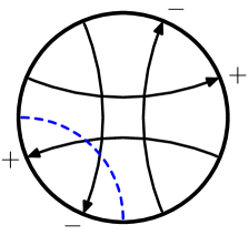
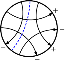
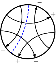
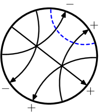
4.99 5.2025 5.2133 5.2160
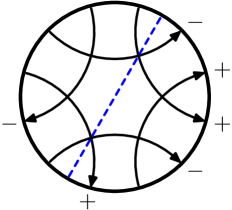
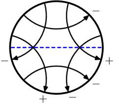
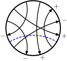
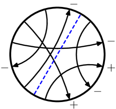
6.72557 6.72975 6.73007 6.73583
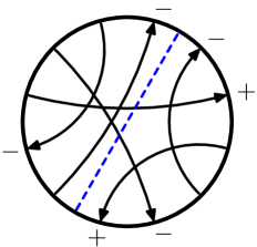
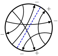
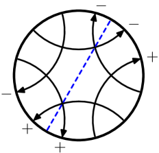
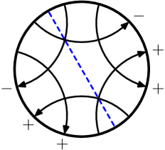
6.75341 6.75348 6.77833 6.77844
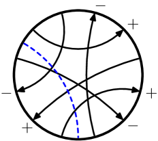
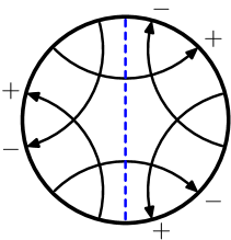
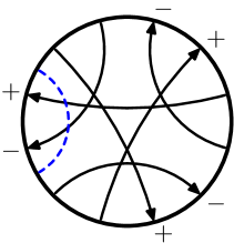
6.79342 6.87269 6.87319
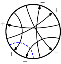
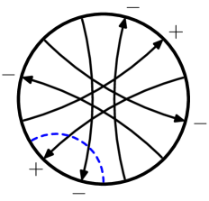
6.89623 6.89815
|
|
| Knot | Seifert matrices |
|---|---|
| 3.6 | |
| 4.99 | |
| 4.105 | |
| 4.108 | |
| 5.2012 | |
| 5.2025 | |
| 5.2080 | |
| 5.2133 | |
| 5.2160 | |
| 5.2331 | |
| 5.2426 | |
| 5.2433 | |
| 5.2437 | |
| 5.2439 | |
| 5.2445 | |
| Knot | Seifert matrices |
|---|---|
| 6.72557 | |
| [0,0,0,0,0,0],[0,0,0,0,0,0]] | |
| [0,0,1,1,0,-1],[0,1,1,0,1,0]] | |
| 6.72692 | |
| 6.72695 | |
| 6.72938 | |
| [0,0,0,0,0,0],[0,0,0,0,0,0]] | |
| [0,0,1,1,0,-1],[0,1,1,0,1,0]] | |
| 6.72944 | |
| 6.72975 | |
| [0,0,0,0,0,0],[0,0,0,0,0,0]] | |
| [0,0,1,1,0,-1],[0,1,1,0,1,0]] | |
| 6.73007 | |
| 6.73053 | |
| 6.73583 | |
| 6.75341 | |
| 6.75348 | |
| 6.77833 | |
| [0,0,0,0,0,0],[0,0,0,0,0,0]] | |
| [0,0,1,1,0,-1],[0,1,1,0,1,0]] | |
| 6.77844 | |
| [0,0,0,0,0,0],[0,0,0,0,0,0]] | |
| [0,0,1,1,0,-1],[0,1,1,0,1,0]] | |
| 6.77905 | |
| 6.77908 | |
| 6.77985 | |
| 6.78358 | |
| Knot | Seifert matrices |
|---|---|
| 6.79342 | |
| 6.85091 | |
| 6.85103 | |
| 6.85613 | |
| 6.85774 | |
| 6.87188 | |
| 6.87262 | |
| [0,0,0,0,0,0],[0,0,0,0,0,0]] | |
| [0,0,1,1,0,-1],[0,1,1,0,1,0]] | |
| 6.87269 | |
| 6.87310 | |
| 6.87319 | |
| 6.87548 | |
| 6.87846 | |
| 6.87857 | |
| 6.87859 | |
| 6.87875 | |
| 6.89156 | |
| 6.89187 | |
| 6.89198 | |
| 6.89623 | |
| 6.89812 | |
| 6.90099 | |
| [0,0,0,0,1,-1],[0,0,0,0,1,0]] | |
| [0,0,0,0,1,0],[0,0,0,1,0,0]] |
| Knot | Seifert matrices |
|---|---|
| 6.90109 | |
| 6.90115 | |
| 6.90139 | |
| 6.90146 | |
| [0,0,0,0,0,0],[0,0,0,0,0,0]] | |
| [0,0,1,1,0,-1],[0,1,1,0,1,0]] | |
| 6.90147 | |
| 6.90150 | |
| 6.90172 | |
| 6.90194 | |
| 6.90195 | |
| 6.90209 | |
| 6.90214 | |
| 6.90217 | |
| 6.90219 | |
| 6.90227 | |
| 6.90228 | |
| 6.90235 | |
| [0,0,0,0,1,0],[1,0,0,0,1,0]] | |
| [0,0,0,-1,1,1],[0,0,0,0,0,0]] |
References
- \ProcessBibTeXEntry \ProcessBibTeXEntry \ProcessBibTeXEntry \ProcessBibTeXEntry \ProcessBibTeXEntry \ProcessBibTeXEntry \ProcessBibTeXEntry \ProcessBibTeXEntry \ProcessBibTeXEntry \ProcessBibTeXEntry \ProcessBibTeXEntry \ProcessBibTeXEntry \ProcessBibTeXEntry \ProcessBibTeXEntry \ProcessBibTeXEntry \ProcessBibTeXEntry \ProcessBibTeXEntry \ProcessBibTeXEntry \ProcessBibTeXEntry \ProcessBibTeXEntry \ProcessBibTeXEntry \ProcessBibTeXEntry \ProcessBibTeXEntry \ProcessBibTeXEntry \ProcessBibTeXEntry \ProcessBibTeXEntry \ProcessBibTeXEntry \ProcessBibTeXEntry \ProcessBibTeXEntry \ProcessBibTeXEntry \ProcessBibTeXEntry \ProcessBibTeXEntry \ProcessBibTeXEntry \ProcessBibTeXEntry \ProcessBibTeXEntry \ProcessBibTeXEntry \ProcessBibTeXEntry \ProcessBibTeXEntry \ProcessBibTeXEntry \ProcessBibTeXEntry \ProcessBibTeXEntry \ProcessBibTeXEntry \ProcessBibTeXEntry \ProcessBibTeXEntry \ProcessBibTeXEntry \ProcessBibTeXEntry \ProcessBibTeXEntry \ProcessBibTeXEntry \ProcessBibTeXEntry \ProcessBibTeXEntry \ProcessBibTeXEntry \ProcessBibTeXEntry \ProcessBibTeXEntry \ProcessBibTeXEntry