Silkswap: An asymmetric automated market maker model for stablecoins
Abstract
Silkswap is an automated market maker model designed for efficient stablecoin trading with minimal price impact. The original purpose of Silkswap is to facilitate the trading of fiat pegged stablecoins with the stablecoin Silk, but it can be applied to any pair of stablecoins. The Silkswap invariant is a hybrid function that generates an asymmetric price impact curve. We present the derivation of the Silkswap model and its mathematical properties. We also compare different numerical methods used to solve the invariant equation. Finally, we compare our model with the well known Curve Finance model.
Keywords: AMM, DEX, stablecoin, hybrid function model, low price impact.
1 Introduction
Decentralized EXchanges (DEXs) are currently the most popular application of Decentralized Finance (DeFi). Unlike centralized exchanges, DEXs are not based on a single centralized entity acting as custodians or intermediaries. Instead, on DEXs traders retain full control of their funds and private keys, and smart contracts execute trades for users in a neutral and automated fashion. Most DEXs use Automated Market Maker (AMM) models to define the rules of trading, rather than relying on the order book model. Liquidity providers can deposit their tokens into liquidity pools in exchange for rewards coming from swap fees and token farming. The AMM algorithmically computes the price of the tokens inside a liquidity pool only based on the token balance. A technical introduction on the mechanics of AMMs can be found in [Angeris and Chitra, 2020] and [Mohan, 2022].
One of the first AMMs to appear in DeFi is Uniswap [Adams, 2018], that together with its upgraded version, Uniswap v2 [Adams et al., 2020], is based on the Constant Product Market Maker (CPMM) model. This model assumes that the product of the quantities of tokens in a liquidity pool is constant, which guarantees infinite liquidity inside the pool. CPMM works quite well for volatile tokens, as it promptly adapts the price in response to new trades. Nevertheless, it is not very suitable when trading low volatility or stable assets.
Another important AMM model is the Constant Sum Market Maker (CSMM), that assumes that the sum of the quantities of tokens inside the pool is constant. The advantage of this model is that any trade has zero price impact, however it also has the inconvenience that it permits the complete drain of the entire liquidity inside the pool. For this reason, it is not used in practical applications.
Low price impact is a good property when swapping between fiat pegged stablecoins. Curve Finance [Egorov, 2019], formerly Stableswap, and the new version Curve v2 [Egorov, 2021] implement a Hybrid Function Market Maker (HFMM) model with the exact purpose of facilitating swaps between stablecoins. This model combines CPMM and CSMM together in order to take advantage of both the infinite liquidity property of CPMM and the zero price impact property of CSMM.
The main goal of the Silkswap model is to facilitate the trades of Silk with other fiat pegged stablecoins.
However this model can be used to trade any pair of stablecoins.
In the current version, it is designed only for two-asset liquidity pools.
Silk [Duniya, 2021] is a privacy-preserving overcollateralized stablecoin developed by Shade Protocol and native to the Secret Network blockchain [Woetzel, 2020].
The main feature of Silk is that it is a stablecoin pegged to a basket of global currencies and commodities using decentralized price feeds,
creating a digital currency that serves as a hedge against single currency volatility.
We developed Silkswap as an HFMM model inspired by the Curve Finance v2 model. Additionally we introduced more flexibility in the shape of the invariant function,
allowing for an asymmetric price impact curve.
In this way, it is possible to discourage possible imbalances within the liquidity pool.
In the next sections we derive the Silkswap invariant and show its mathematical properties. We present numerical results for
three different zero-finder algorithms and finally we compare our model with the Curve finance model.
2 Silkswap model
Let us consider a liquidity pool containing only two stablecoins.
The two tokens in focus are token , that represents any fiat pegged stablecoin, and token that represents Silk.
We use lower-case letters and to indicate the quantities of and .
Without loss of generality, let us quote the price of and in US dollars, although any other fiat currency would work.
Let us introduce the conversion factors and , such that
the values in dollars of and are simply and respectively.
The conversion factor has units [USD]/[X] and has units [USD]/[Y].
We also introduce , the conversion factor between and , which has units [X]/[Y].
The conversion factors and represent the market prices of one unit of and respectively, while
is the price of one unit of in terms of .
These values must be provided by an oracle, which is an external source of information that is fed into the AMM smart contract with a certain
frequency.
Example:
Let us consider a liquidity pool containing USDC (token ) and Silk (token ).
If the oracle price of Silk is 1.05$ then ,
while for USDC the oracle price is exactly 1$,
resulting in a perfect peg, then we have . The direct conversion between Silk and USDC is therefore .
Later we will often identify with USDC and with SILK to make the discussion clearer.
Let us define the equilibrium point in a liquidity pool as the point where the dollar value of equals the dollar value of . The equilibrium point satisfies the equilibrium equation
| (1) |
From now on, we will assume that is our numeraire, and we will express the value of in terms of . The equilibrium equation becomes
| (2) |
This choice is due to the fact that it is more natural for the user to evaluate an asset in terms of a fiat pegged stablecoin. Because Silk is pegged to a basket, its value expressed in terms of any fiat currency is not stable, but it fluctuates with a very low volatility.
2.1 Silkswap invariant
Under the CPMM model, the quantities and must satisfy the following equation:
| (3) |
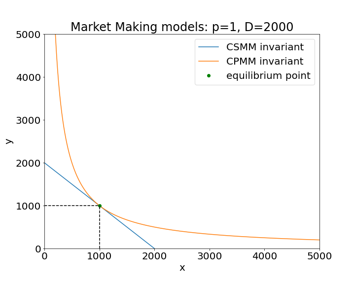
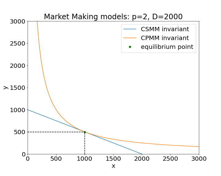
with constant. The equilibrium point, satisfying both (2) and (3), is . Under the CSMM model instead, the following equation holds:
| (4) |
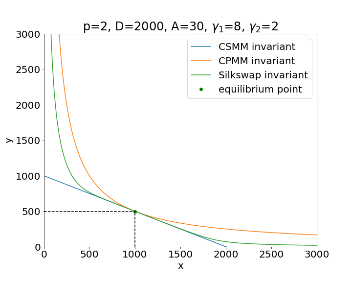
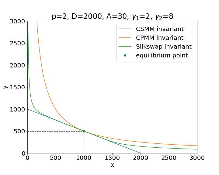
with constant. The equilibrium point, satisfying (2) and (4), is . The equilibrium point is a fundamental point where the ratio of the quantities of tokens in the pool is equal to , and any invariant curve should contain this point. Since this point is unique, it follows that . In figure 1 we can see the graph of these two models, with different values of .
Now let us consider the following linear combination of the CSMM and CPMM models. Let us multiply Eq. (4) by , and sum it with eq. (3):
| (5) |
where is a function of and , defined as
| (6) |
and
| (7) |
and the other parameters are constants satisfying , , .
Let us remark that is an adimensional quantity and has the same dimension of .
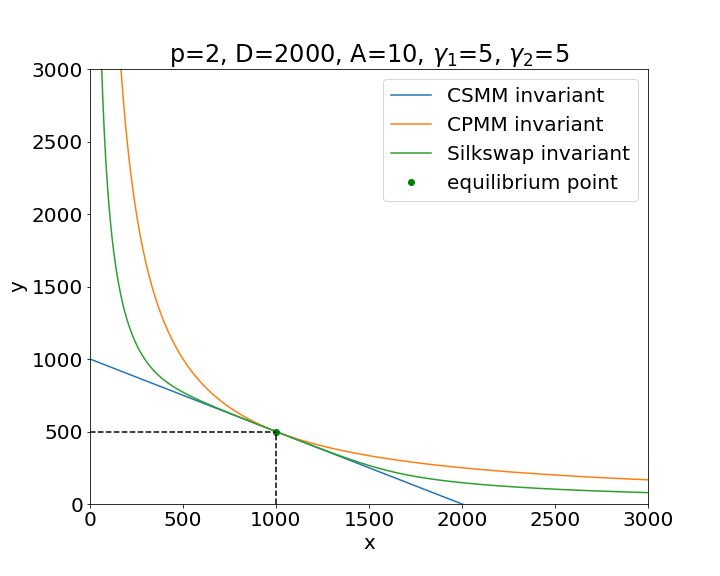
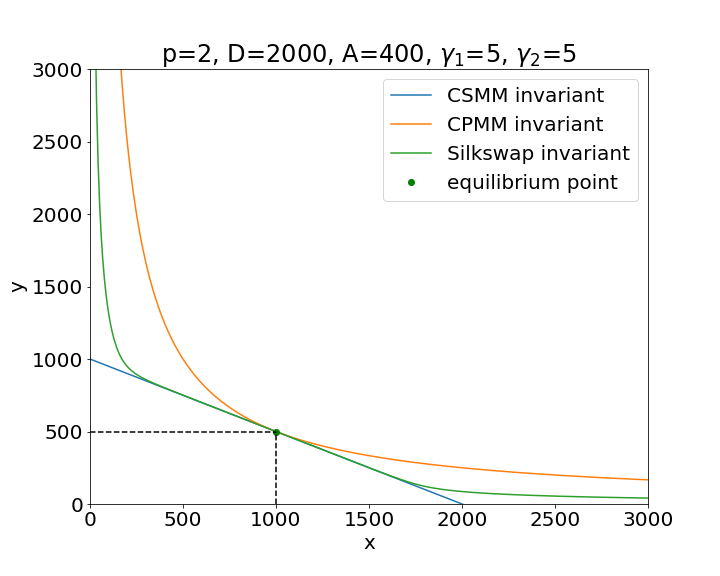
We call the equation (5), together with (6) and (7), the Silkswap invariant.
The graph of the Silkswap invariant is shown in figures 3 and 3 under different set of parameters.
We can see that the CPMM hyperbola is always greater than the CSMM line, and they touch each other at the equilibrium point. The Silkswap invariant graph
lies in between them. In the Appendix we prove these facts in the theorems (A.1) and (A.3).
The parameter tells us how close the Silkswap graph is to the CPMM or to the CSMM.
From Eq. (5) we can easily see that for the invariant converges to the CPMM curve, while for it converges to the CSMM curve.222The parameter
has the same meaning of the parameter in the Stableswap model [Egorov, 2019].
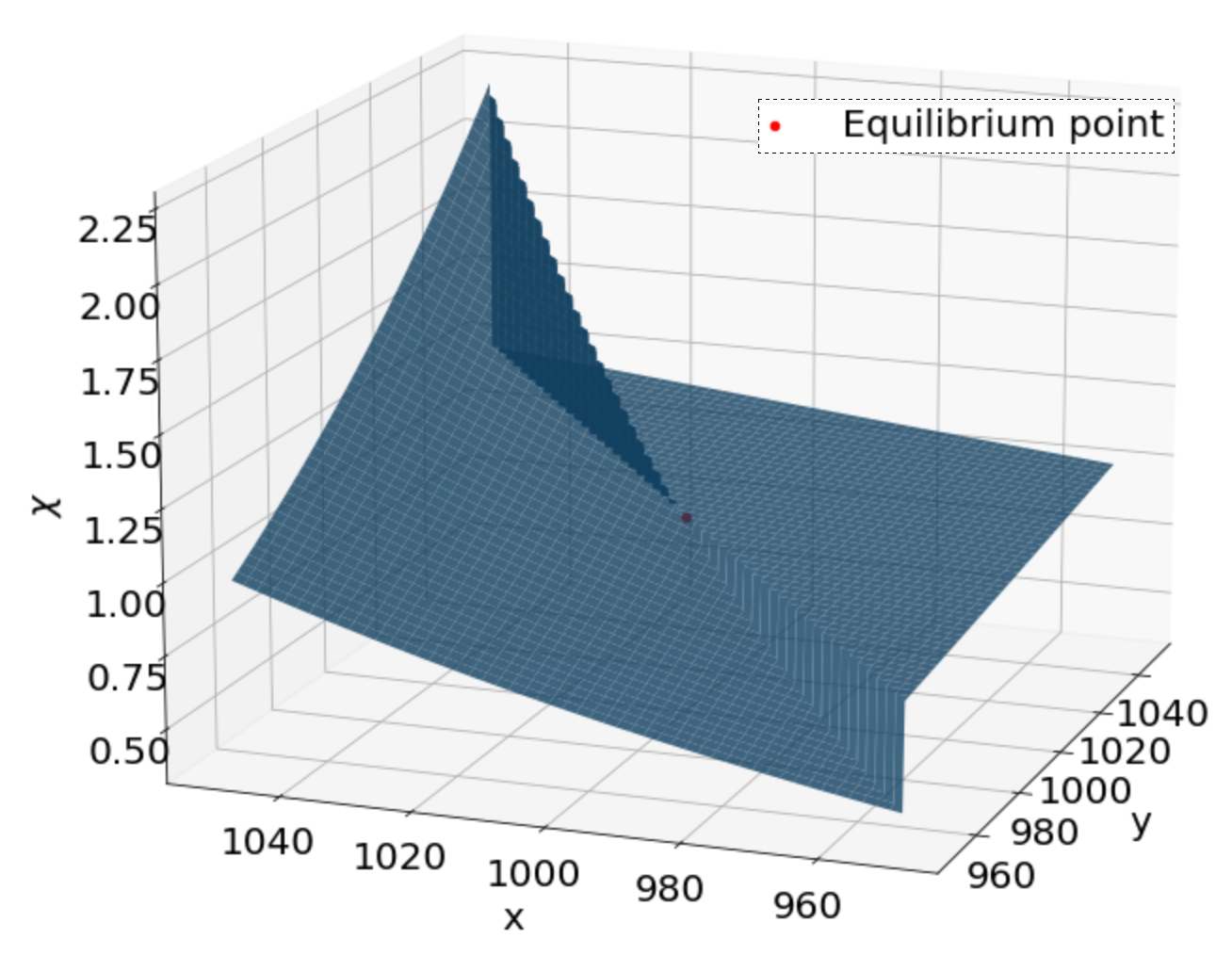
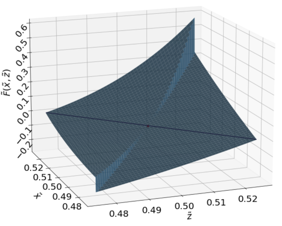
The two dimensional function in (6) is a discontinuous function. We show the surface plot in Fig. (4).
In the Appendix we prove that, although the Silkswap invariant contains a discontinuous function, the points of our interest are regular points where the invariant is
continuously differentiable.
2.2 Pricing with the Silkswap invariant
In order to compute the price of a token, it is convenient to express the invariant in the explicit form , where is continuously differentiable, decreasing and convex 333The set is the set .. For the CPMM the explicit form is the hyperbola , while for the CSMM the explicit form is the straight line , defined for .
If we trade an infinitesimal quantity , using the first order Taylor approximation , it results equal to trade the quantity . Let us recall that by definition , so we need to use the absolute value to define a positive price. We define the current price of the token as function of
| (8) |
The price of the token is defined as:
| (9) |
Under the CPMM model, the current price is , and at equilibrium .
Under the CSMM model, the current price is a constant value, , for any .
Unfortunately the Silkswap invariant cannot be written in an explicit form. We can define the function as
| (10) |
with as in (7). The Silkswap invariant (5) is the set of points that satisfy
| (11) |
The partial derivatives are:
| (12) | ||||
| (13) |
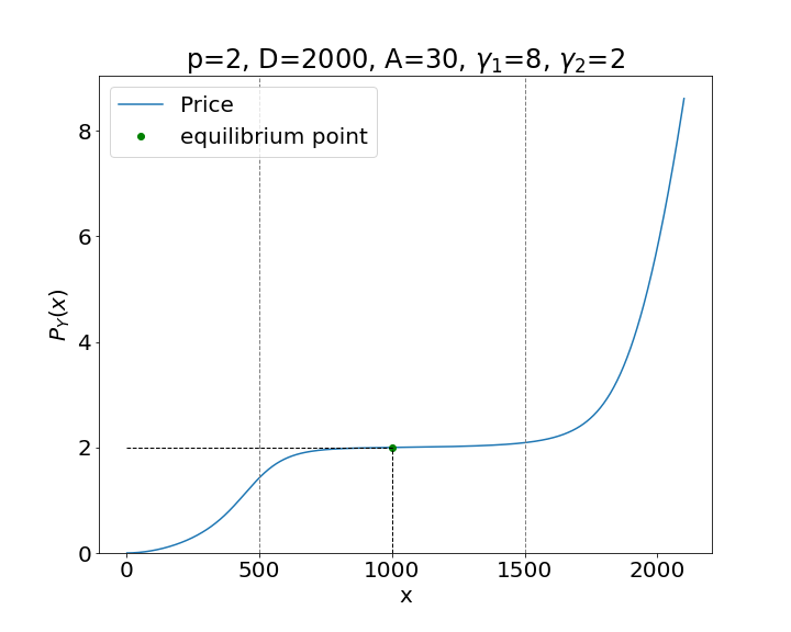
Thanks to the Theorem (A.6), we know the expression of the slope of the Silkswap invariant, which can be used to compute the prices of the tokens by (8) and (9). The slope has the following expression:
| (14) |
In Figure 5 we present two examples of price curves obtained from this expression.
2.3 Scaled invariant
If we consider the function (10) depending also on , for any constant we have
| (15) |
This means that the Silkswap invariant is also invariant by scaling.
This property is very useful in practice because it reduces the convergence time of some numerical methods
and prevents possible overflows when the variables have very high magnitudes.
Let us introduce the variable .
We can consider with , equal to , and define the corresponding scaled function:
| (16) |
where , and . We show in Fig. 6 the graph of this function. The scaled Silkswap invariant is given by
| (17) |
The function (16) is related with (10) by
| (18) |
Using the chain rule
| (19) | |||
| (20) |
we can rewrite the price equation (14) as
| (21) |
In the numerical calculation of the swap amount, we will make use of the scaled function (16), rather than (10), because it reduces a lot the number of operations, and consequently the run time and gas fees.
3 Numerical implementation
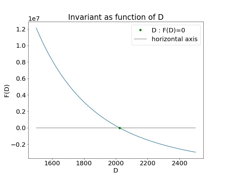
3.1 Calculation of D
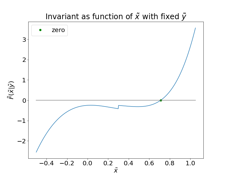
RIGHT: Scaled invariant as function of . We used , , , , , . The function has only one zero.
RIGHT: Scaled invariant as function of . We used , , , , , . The function is increasing for , therefore the Halley and Newton methods converge to the right solution.
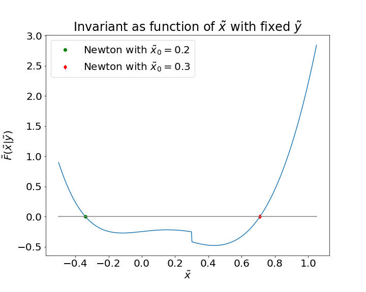
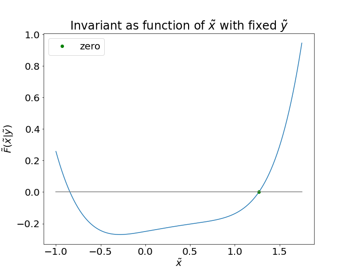
Since this model is defined by an implicit equation, we need numerical methods to compute the variables of interest. If the amounts of tokens in the pool satisfy the equilibrium equation 2, then the parameter can be quickly computed from Eq. (4). However, it is quite rare that a liquidity pool is in perfect equilibrium and the equation 2 is almost never satisfied. In this cases we need to compute from Eq. (5) using a numerical method. Let us define as the function (10) when we consider variable and , fixed. With an abuse of notation we can call it ”invariant function dependent of ”, but let us recall that the name invariant can be used only when . In Fig 8, we can see that is a smooth decreasing function. We compare three different numerical methods: the Newton method, Halley method and the bisection method, see Table 1.
| Pool with 2000 USDC and 1000 SILK | |||
| Starting point | Method | Iterations | Time |
| 2AM | Newton | 4 | 312.8µs |
| 2GM | Newton | 8 | 770.4µs |
| 2AM | Halley | 2 | 390.5µs |
| 2GM | Halley | 5 | 820.4µs |
| / | Bisection | 61 | 2.37ms |
| Pool with 200000 USDC and 100000 SILK | |||
| Starting point | Newton | Halley | Bisection |
| 2AM | Newton | 4 | 290.0µs |
| 2GM | Newton | 7 | 790.3µs |
| 2AM | Halley | 3 | 399.5µs |
| 2GM | Halley | 5 | 914.2µs |
| / | Bisection | 67 | 2.6ms |
The idea of using two times arithmetic mean (AM) and geometric mean (GM) as starting points for Newton and Halley methods comes from Theorem A.4.
We can see that 2AM is a better choice.
Although Newton method has more loop iterations than Halley, it performs better in terms of time. The reason is that the calculation of the second derivative is more expensive,
in terms of operations, than the extra iterations. The expression of the derivatives are in Appendix B.
Bisection method, as expected from theoretical results, is the slowest.
| Pool with USDC and SILK | |||
| Swap size | Method | Iterations | Time |
| 0 | Bisect | 0 | 153µs |
| Bisect | 52 | 1.32ms | |
| Bisect | 52 | 1.31ms | |
| Bisect | 52 | 1.30ms | |
| Bisect | 52 | 1.37ms | |
| Bisect | 52 | 1.31ms | |
| Bisect | 52 | 1.34ms | |
| Bisect | 52 | 1.47ms | |
| Bisect | 52 | 1.46ms | |
| 0 | Halley | 0 | 190µs |
| Halley | 2 | 311µs | |
| Halley | 2 | 303µs | |
| Halley | 3 | 366µs | |
| Halley | 4 | 436µs | |
| Halley | 9 | 751µs | |
| Halley | 17 | 1.30ms | |
| Halley | 26 | 1.95ms | |
| Halley | 37 | 2.88ms | |
| 0 | Newton | 0 | 159µs |
| Newton | 3 | 262µs | |
| Newton | 3 | 246µs | |
| Newton | 4 | 285µs | |
| Newton | 6 | 358µs | |
| Newton | 16 | 674µs | |
| Newton | 30 | 1.20ms | |
| Newton | 49 | 2.01ms | |
| Newton | 68 | 2.80ms | |
| Pool with USDC and SILK | |||
| Swap size | Method | Iterations | Time |
| 0 | Bisect | 0 | 141µs |
| Bisect | 52 | 1.51ms | |
| Bisect | 52 | 1.45ms | |
| Bisect | 52 | 1.62ms | |
| Bisect | 52 | 1.46ms | |
| Bisect | 52 | 1.48ms | |
| Bisect | 52 | 1.46ms | |
| Bisect | 52 | 1.57ms | |
| Bisect | 52 | 1.47ms | |
| 0 | Halley | 0 | 150µs |
| Halley | 1 | 270µs | |
| Halley | 1 | 269µs | |
| Halley | 2 | 346µs | |
| Halley | 2 | 341µs | |
| Halley | 2 | 341µs | |
| Halley | 3 | 422µs | |
| Halley | 4 | 488µs | |
| Halley | 9 | 885µs | |
| 0 | Newton | 0 | 155µs |
| Newton | 2 | 236µs | |
| Newton | 2 | 239µs | |
| Newton | 2 | 247µs | |
| Newton | 3 | 297µs | |
| Newton | 3 | 284µs | |
| Newton | 4 | 316µs | |
| Newton | 6 | 394µs | |
| Newton | 16 | 1.04ms | |
3.2 Calculation of the swap amount
We will also make use of numerical methods to calculate the amount of tokens that are returned during a swap.
When a quantity is introduced into the pool, we need to compute the quantity that is
extracted from the pool, and such that the point belongs to the Silkswap invariant.
The parameter is fixed, and it is irrelevant for this calculation, therefore in order to simplify the problem,
we can use the scaled function (16).
Let us define and the function with or fixed respectively.
Again, with an abuse of notation
we can call these functions ”invariant functions depending on or ”.
In the following we consider the case when is extracted and therefore we need to find the zero of , but the same analysis works for
.
In the Figures 8 and 8, we can see that the function is discontinuous and can have different shapes depending on the choice of the parameters.
So the numerical convergence to the right solution is not always guaranteed.
By definition, the parameter can be any non-negative real number. In practice we restrict to be a positive integer value in order to simplify the model.
The value of is particularly important because it controls the behavior of the left tail:
as we can see if we compare the plot of in Fig. 8 with the plots in Fig. 8.
When is odd, has two zeros. Since by definition, we know that the correct solution must be positive.
However, numerical methods such as Newton and Halley can converge to the wrong solution if initialized with an unlucky starting point, see Fig. 8 (LEFT).
Under some set of parameters, it is possible that the function is increasing for ,
and the Newton method works fine, see Fig. 8 (RIGHT).
However, to avoid this uncertainty, in these cases it is better to use numerical methods that always guarantee the convergence to the right solution, such
as the bisection algorithm. If we call the amounts in the pool before the swap,
and the amounts after the swap such that ,
then we know that . The swap amount is therefore .
In practical applications we want to take advantage of the speed of the Newton method, and therefore we choose to use only odd values for .
For comparisons between the three numerical methods under consideration, see Table 2.
Let us comment a few points:
-
1.
The number of iterations of the bisection method does not depend on the size of the pool. The reason is that we are searching in the interval , and . In the example, since we are at equilibrium and therefore .
-
2.
The number of iterations of the bisection method does not depend on the size of the trade either.
-
3.
As for the calculation of , Newton is slightly faster than Halley. The computation of second order derivatives (see Appendix B) is expensive.
-
4.
The number of iterations of the Newton method increases when the size of the trade is big with respect to the size of the pool. In this case the Newton method is the one that performs worse while the bisection method is the one that performs best. However, in practice it is very unlikely to see transactions bigger than the size of the pool.
-
5.
We used i.e. the value before the swap, as an initial guess. We tried also with and as initial guesses, but the performances are worse.
When considering an even , it turns out that the Newton method is superior for both the calculations of and the swap size. In production, we decided to use Newton as main solver, and bisection as fallback in case of failure.
3.3 Model implementation
We tested the model with values of ranging from 1 to and values of gamma from to , under a variety of conditions including pool sizes from 1 to USDC total value, with a similar range of trade sizes. Generally, the Rust implementation can handle trade sizes several orders of magnitude above the size of the pool without overflowing, unless the values for or are excessively high. Since and are exponents, large values quickly create unmanageable numbers.
We implemented the Silkswap algorithm inside Rust smart contracts on the Secret Network blockchain. Smart contract do not allow floating point calculations, and this required the use of a few workarounds. Since smart contracts only support integer arithmetics, we stored most numbers as larger than their actual value. This effectively allowed us to store 18 decimal places. Variables are stored as uint256 i.e. unsigned 256 bits integers. Additionally, we paired each variable with a boolean representing its sign, allowing us to calculate both positive and negative numbers. The square root in 2GM is computed by the Babilonian method.
3.4 Parameter selection
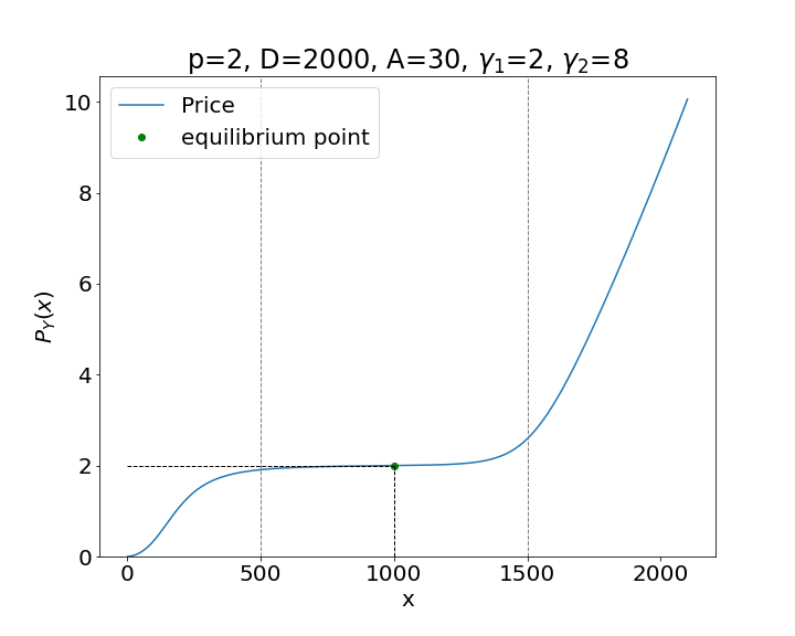
In the previous sections we have seen how the parameters , and modify the shape of the Silkswap invariant. Specifically, parameter controls the flatness of the curve in the area around the equilibrium point (see Fig 3), while the parameters and are used to control the curvature and asymmetry of the invariant (see Fig 3). The shape of the invariant is directly reflected in the price curve (see Fig. 5). Thus, the parameters of the model must be chosen in such a way as to make the price curve attractive for DEX users. Therefore, they must maintain a low price impact and protect against possible imbalances in the liquidity pool.
In this section we present a practical method for deciding the value of parameters.
Since it is not very practical to consider a curve that depends on the quantity of tokens in the liquidity pool,
we define the fraction of token inside the pool as and similarly we define the fraction of token as
. As usual we multiply by to have the same units as .
It is very convenient to express the price curve as a function of the fraction, because the fraction is a percentage and does not depend on the size of the pool.
Now we can choose a level of price impact that suits us, and choose the parameters in such a way that the price is impacted by this price impact
at a certain level of fraction of the tokens.
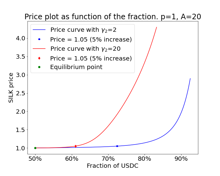
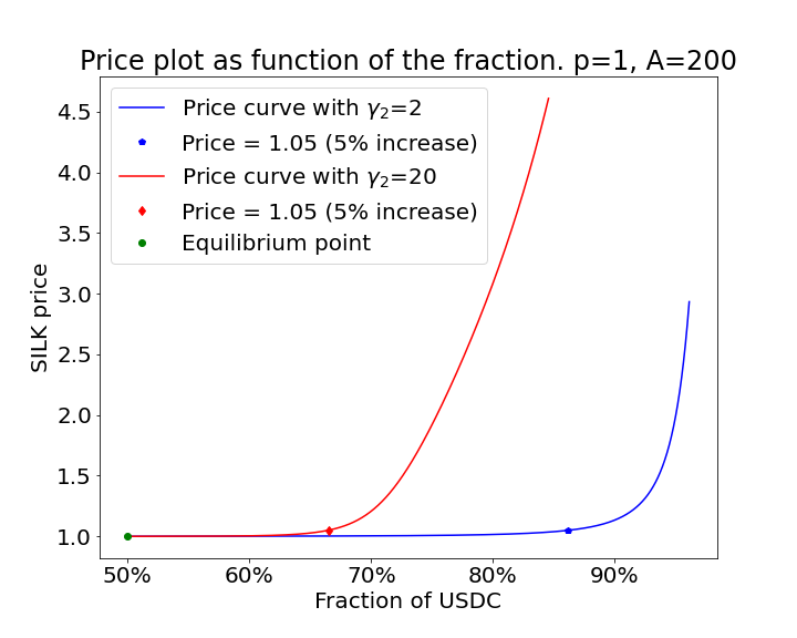
In Fig. 9, we show examples of price curves for different parameter values. We choose a 5% level of price impact for .
We are considering the case such that we are able to calculate . The same procedure should also be done for and considering a price impact
for in order to find .
In this example, the price of the token (SILK) at equilibrium is . Its value after the 5% price impact increase is and it is represented by the points
on the price curves in the figure.
We can see how by changing and it is possible to move the point
to the right or to the left as desired.
A look at the curvature can also be helpful in choosing these parameters.
4 Comparison with the Curve model
Curve finance is currently the most popular DEX for trading stablecoins. The Curve v2 model [Egorov, 2021] is an HFMM model, conceptually not very different from Silkswap. They both take a linear combination of the CSMM and the CPMM models. Since in the development of Silkswap we took inspiration from Curve, we decided to use a similar notation. The parameter in Curve has the same meaning as in Silkswap. The main difference between these models is the definition of the function :
For simplicity we didn’t include the conversion factor . In both models . If for a moment we do not consider the fact that our gamma can assume two values, the gammas in the two models have different meanings. For any point not at equilibrium, in Silkswap: and , while for Curve v2 we have the opposite: and .
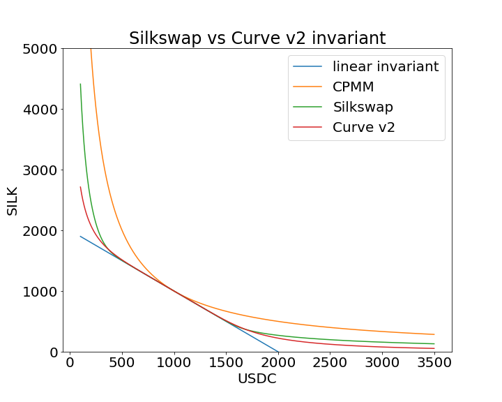
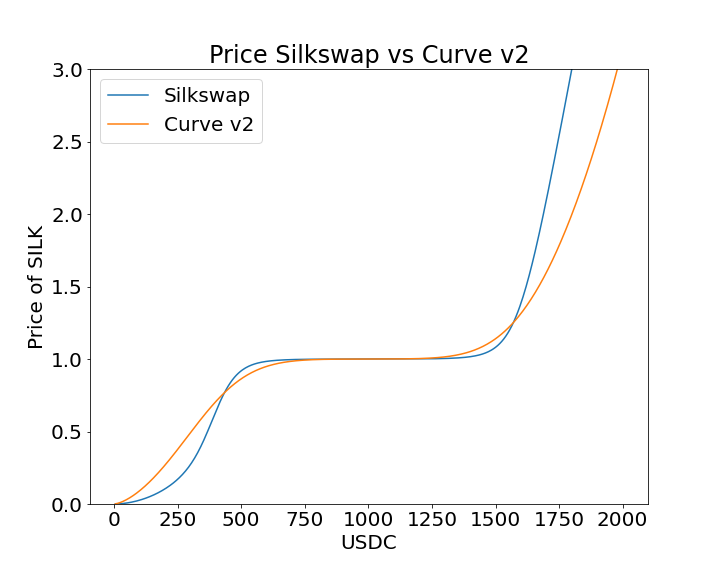
In Fig. 10 we can see the invariant and price curves produced by these two models. The values of gammas are chosen to make the two curves as close as possible when using same value of . We notice that the Silkswap model produces a higher curvature, although we did not prove it formally.
Another difference between the models is that currently Silkswap is designed to work with liquidity pools containing only two tokens, while Curve v2 can have pools with any number of coins.
Unlike Curve, we have decided to apply transaction fees to the token that is inserted into the pool, following the same approach used by Uniswap and Osmosis.
5 Conclusions
The Silkswap invariant is an AMM model that allows users to trade stablecoins with minimal price impact when the state of the pool is close to equilibrium. Away from equilibrium, the price impact tends to that of the CPMM model. The main innovation of this model is the asymmetry of the invariant, which helps to regulate the liquidity in the pool and discourage strong imbalances in the quantity of tokens asymmetrically. For new stablecoins like Silk that are in the process of building up liquidity, the asymmetric curve provides attack protection, discouraging the sale when the amount of Silk in the pool exceeds a certain threshold (dependent on the parameters of the model). This is done by making the price impact grow faster in that direction and slower in the opposite. Figure 5 shows this behavior very well.
Acknowledgements
This research was fully funded by Shade Protocol.
Appendix A Properties of the Silkswap invariant
In Figure 1 we can see that the CPMM graph is greater than the CSMM graph, and they intersect each other at the equilibrium point. Let us formally prove this fact.
Theorem A.1.
For , the condition
| (A.1) |
is always satisfied.
Proof.
Theorem A.2.
The value of , defined in (6) always satisfy
| (A.2) |
Proof.
Since is a function of only positive variables, it follows that must be positive.
Let us consider the Silkswap invariant (5):
| (A.3) |
Since the sum of two terms is zero, it means that or both terms are zero, or the two terms have opposite sign.
The case of both terms equal zero happens only at the equilibrium point.
Let us consider the case of both terms different than zero. We want to prove by contradiction that the first term must be positive.
If the first term is negative, then , and we have that
by Theorem A.1. This implies that , but this is a contradiction because the terms must have opposite sign. The second term is always negative or zero, and we can conclude the proof.
∎
In Figure 3 we can see that the Silkswap invariant always lies between the graphs of the CSMM and CPMM models.
Theorem A.3.
The graph of the Silkswap invariant always lies between the graphs of the CSMM and CPMM models.
Proof.
First we prove that the Silkswap invariant graph is not greater than the CPMM graph. This is a direct consequence of Theorem A.2:
| (A.4) |
Now we prove that the Silkswap invariant graph is not smaller than the CSMM graph. Let us consider the invariant (5) and divide it by the positive quantity . We get
where we used . It follows that
| (A.5) |
∎
Theorem A.4.
The parameter in the Silkswap invariant satisfies
| (A.6) |
where GM is the geometric mean of and , and AM is the arithmetic mean.
Proof.
Theorem A.5.
Proof.
We present a proof for only, since the same arguments can be used for . Let us consider the expression:
Since all variables are positive, when then . This happens for .
For , let us rearrange the terms inside the square brackets and use (A.5):
This last inequality proves the theorem. ∎
Unfortunately, the function defined in (10) is not continuous in the entire , and we need to be careful around the points of discontinuity. The following theorem guarantees the validity of (14).
Theorem A.6.
The derivative of the Silkswap invariant can be written as
Proof.
The function is continuously differentiable everywhere except on the line , where it is discontinuous. The intersection between this line and the Silkswap invariant,
corresponds to the equilibrium point . At the equilibrium point we have
from any directions, and therefore is continuous in this point. Also
with limits from any directions. Therefore the partial derivatives are continuous and is continuously differentiable at .
Let us differentiate along the direction of the Silkswap invariant
In the Theorem (A.5) we prove that . We can rearrange the last expression to conclude the proof. ∎
Appendix B Expression of the derivatives
Derivative expressions used for the calculation of by Newton and Halley methods:
| (B.1) |
| (B.2) |
First derivative expressions for computing and by Newton and Halley methods:
| (B.3) |
| (B.4) |
for
| (B.5) |
Second derivatives:
| (B.6) |
| (B.7) |
References
- [Adams, 2018] Adams, H. (2018). Uniswap v1 whitepaper. https://hackmd.io/@HaydenAdams/HJ9jLsfTz.
- [Adams et al., 2020] Adams, H., Zinsmeister, N., and Robinson, D. (2020). Uniswap v2 core. https://uniswap.org/whitepaper.pdf.
- [Angeris and Chitra, 2020] Angeris, G. and Chitra, T. (2020). Improved price oracles: Constant function market makers. Proceedings of the 2nd ACM Conference on Advances in Financial Technologies, pages 80 – 91.
- [Duniya, 2021] Duniya, S. (2021). Silk: A privacy-preserving algorithmic burn stablecoin. https://shadeprotocol.io/pdf/Silk_Whitepaper.pdf.
- [Egorov, 2019] Egorov, M. (2019). Stableswap - efficient mechanism for stablecoin liquidity. https://curve.fi/files/stableswap-paper.pdf.
- [Egorov, 2021] Egorov, M. (2021). Automatic market-making with dynamic peg. https://curve.fi/files/crypto-pools-paper.pdf.
- [Mohan, 2022] Mohan, V. (2022). Automated market makers and decentralized exchanges: a defi primer. Financial Innovation, 8(20).
- [Woetzel, 2020] Woetzel, C. (2020). Secret network: A privacy-preserving secret contract & decentralized application platform. https://www.securesecrets.org/Secret_Network_Graypaper_2.0.1_1.pdf.