SiML: Sieved Maximum Likelihood for Array Signal Processing
Abstract
Stochastic Maximum Likelihood (SML) is a popular direction of arrival (DOA) estimation technique in array signal processing. It is a parametric method that jointly estimates signal and instrument noise by maximum likelihood, achieving excellent statistical performance. Some drawbacks are the computational overhead as well as the limitation to a point-source data model with fewer sources than sensors. In this work, we propose a Sieved Maximum Likelihood (SiML) method. It uses a general functional data model, allowing an unrestricted number of arbitrarily-shaped sources to be recovered. To this end, we leverage functional analysis tools and express the data in terms of an infinite-dimensional sampling operator acting on a Gaussian random function. We show that SiML is computationally more efficient than traditional SML, resilient to noise, and results in much better accuracy than spectral-based methods.
Index Terms— stochastic maximum likelihood, sieved maximum likelihood, spatially extended sources, random fields, sampling operator, array signal processing.
1 Introduction
Array signal processing [1, 2, 3] is primarily concerned with the sensing, processing and estimation of random wavefields (electromagnetic or mechanic). Techniques from array signal processing are used in myriad of applications, including for example acoustics [4, 5], radio-interferometry [6, 7], radar and sonar systems [2, 8], wireless networks [9, 10, 11], and medical imagery [12, 13]. The sensing devices in all those applications consist of large networks of sensors, called sensor arrays or phased-arrays.
A common task in array signal processing consists of estimating the intensity field of an emitting wavefield. The various algorithms available in the literature for this purpose divide into two categories [1]: spectral-based and parametric methods. Spectral-based ones estimate the intensity field by “steering” the array towards particular directions in space and evaluating the output power. The intensity field is thus recovered sequentially by scanning via beamforming [1, 8, 11] a grid covering the field of view. Famous beamformers include Bartlett, also known as Matched Beamforming (MB), and Capon, which is often called Minimum Variance Distortionless Response (MVDR) [1]. These are extremely simple to implement, computationally attractive, and quite generic with little structural or distributional assumptions on the sensed wavefield. They are however limited in terms of accuracy, in particular for extreme acquisition conditions such as small sample size, low signal-to-noise ratio and/or spatial correlation in the wavefield [1].
Parametric methods, on the other hand, attempt to overcome those limitations using a statistical model for the instrument noise and the unknown wavefield. Typically, the thermal noise at each sensor is modelled as an additive Gaussian white random process while the wavefield is assumed to be the incoherent sum of point sources with amplitudes distributed according to a multivariate complex Gaussian distribution, where is strictly smaller than the total number of sensors composing the array. In this context the problem of estimating the intensity field is generally referred to as a direction of arrival (DOA) estimation problem [1].
By thus specifying the data model, parametric methods can achieve much better recovery performance, both theoretically and in practice [1]. Stochastic Maximum Likelihood (SML) [1, 14, 15] is perhaps the most well-known parametric method. It uses explicit maximum likelihood expressions [16] to estimate the various parameters involved in the traditional point-source model [1, 14], namely the noise and sources power as well as the directions of arrival. Each parameter is estimated consistently and general theory of maximum likelihood guarantees efficient estimation as the number of samples grows to infinity.
These strong theoretical guarantees and excellent empirical performance come however at the cost of very intense computation [1]. Moreover, the data model assumptions restrict its application to point sources, of which there must be fewer than the number of sensors, preventing its use in many applications.
This is particularly true for radio-astronomy [6, 7], where the number of sources is typically far larger than the number of antennas forming the array. Moreover, the increased resolution of modern radio-interferometers [17, 18] permits celestial sources with spatial extent and complex shapes to be resolved, for which a point-source model is overly simplistic.
The present work, SiML, takes a maximum likelihood approach based on more general functional data model, which, in particular, allows potentially correlated sources with spatial extent and arbitrary shapes to be recovered.
To this end, we leverage functional analysis tools [19, 20] and formulate the data in terms of an infinite-dimensional sampling operator [19] acting on the wavefield’s amplitude function, modelled as a complex Gaussian random function [21]. Based on this data model, we derive a joint maximum likelihood estimate for both the covariance kernel of this random function and the sensor noise power.
As the optimisation problem elicits many solutions, we deploy the method of sieves [22, 23] as a means of restricting the optimisation problem to a lower dimensional subspace.
For identifiability, we show that this subspace must have a smaller dimension than the total number of sensors in the array.
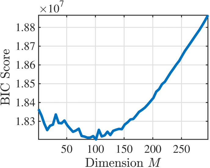
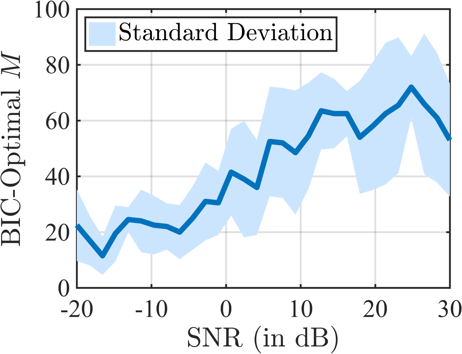
A suitable subspace dimension is obtained by trading off between likelihood improvement and model complexity through the Bayesian Information Criterion (BIC) [24]. Simulations reveal that the subspace dimension acts as a regularisation parameter, increasing or decreasing with the SNR.
For a known noise level, the resulting estimate of the covariance field is shown to be an unbiased, consistent and asymptotically efficient estimate of a particular oblique projection of the true covariance field. The method is computationally far more efficient than traditional SML and resilient to noise. Finally, we demonstrate by simulation that SiML obtains much better accuracy and contrast than spectral-based methods.
2 A Functional Data Model
To allow for the handling of very general sources, we introduce in this section a functional data model. Leveraging tools from functional analysis [19, 25], the sensing device can be modelled as an infinite dimensional sampling operator acting on an unknown random amplitude function (see [21] for an introduction to random functions). We first investigate the population version of the data model, where the covariance matrix of the instrument recordings is known, before presenting its empirical counterpart, where the covariance matrix is estimated from i.i.d. observations. More details on the modelling assumptions can be found in [1, 14, 26, 3].
2.1 Population Version
Consider an array of sensors with positions . Assuming the emitting sources are in the far-field [3] of the sensor array, they can be thought of as lying on the unit sphere . To allow for arbitrary numbers of complex sources, we consider a notional continuous source field covering the entire sphere, with an associated amplitude function, describing for each direction the emission strength of the source field. In practice, source amplitudes fluctuate randomly [1, 14], and the amplitude function can be modelled as a complex random function , where is some probability space. More precisely, we assume to be a Gaussian random function [21], i.e., that all its finite marginals have distribution:
where denotes the -variate centrally symmetric, complex Gaussian distribution [27, 28], and is some valid covariance matrix depending on the set .
From the Huygens-Fresnel principle [29], exciting the source field with a narrowband waveform of wavelength results in a diffracted wavefront, which, after travelling through an assumed homogeneous medium is recorded by the sensor array. In a far-field context, the Fraunhofer equation [29, 3] permits this wavefront at each sensor position to be approximated by:
| (1) |
where and is an additive white noise term capturing the inaccuracies in measurement of each sensor, distributed as [1]
Noise across sensors is assumed to be identically and independently distributed and independent of the random amplitude function .
We assume that every realisation, or sample function [21], of is an element of some Hilbert space of finite-energy functions, and thus Eq. 1 can be written as:
where which in turn can be re-written more compactly using an analysis operator [19] , mapping an element of to a finite number of measurements:
We call the sampling operator [19] associated with the sensor array. As the sum of two independent centred complex Gaussian random vectors, the vector of measurements is also a centred complex Gaussian random vector with covariance matrix
| (2) |
where denotes the Kronecker delta and is the covariance kernel [21] of :
Introducing the associated covariance operator :
we can again reformulate Eq. 2 in terms of the sampling operator and its adjoint, called the synthesis operator [19], :
| (3) |
By analogy with the finite dimensional case [30], it is customary to write where the operator maps an infinite-dimensional linear operator onto its associated kernel representation. Because of the Gaussianity assumption, the covariance kernel (or equivalently the covariance operator ) completely determines the distribution of . Our goal is hence to leverage Eq. 3 in order to form an estimate of from the covariance matrix of the instrument recordings. Often the source field is assumed to be spatially uncorrelated, in which case the random function is Gaussian white noise [21] and becomes diagonal. The diagonal part of
is called the intensity function of the source field, of crucial interest in many array signal processing applications.
2.2 Empirical Version
In practice of course, the covariance matrix needs to be estimated from a finite number of i.i.d. observations of , say . Typically, the maximum likelihood estimate of is formed by It follows a -variate complex Wishart distribution [27, 31] with degrees of freedom and mean :
| (4) |
The density of a complex Wishart distribution can be found in [31]. In the next section, we use it to form the likelihood function of the data and derive maximum likelihood estimates of the covariance kernel and the noise level .
3 Sieved Maximum Likelihood
We now take the population and empirical data models Eqs. 3 and 4 and derive maximum likelihood estimates for and . The simpler case of known noise power, which allows for an insightful geometric interpretation of the maximum likelihood estimate in terms of projection operators, is presented first. That is then followed by the more general case given an unknown noise level.
3.1 A Constrained Log-Likelihood Maximisation Problem
The log-likelihood function for and given the sufficient statistic [32] can be written in terms of the density function of the complex Wishart distribution [31],
| (5) |
where the terms independent of and have been dropped. As , it is guaranteed that the matrix is invertible and that the log-likelihood function is hence well-defined. Maximum likelihood estimates for and are then obtained by maximising Eq. 5 with respect to and . Since the sampling operator has finite rank and consequently a non-trivial kernel, the log-likelihood function admits infinitely many local maxima. Indeed, for , adding a kernel of the form111The tensor product is defined as . to in (5) does not change the value of the log-likelihood function. We thus choose to impose a unique maximum by restricting the search space for to a lower dimensional subspace, and look for solutions in the range of some synthesis operator , which will be specified in Section 3.4:
where is a Hermitian symmetric matrix and , are the analysis and synthesis operators associated with the family of functions . This regularisation of the likelihood problem by restricting the parameter space to a lower dimensional subspace is generally known as the method of sieves [22, 23]. The maximum likelihood estimates of and are then given by minimising the negative log-likelihood:
| (6) |
where is the so-called Gram matrix [19], given by . For Eq. 6 to admit a unique solution, it is necessary to have at least as many measurements as unknowns. When the noise power is unknown a priori, this requires that . When the noise power is known, there is one less unknown, leading to . This is however not a sufficient condition for identifiability, and we must further assume to be of full column-rank. If the latter condition is verified, we say that the two families of functions and are coherent with one another.
3.2 Estimation with Known Noise Power
Suppose the noise power is known. Then becomes the only variable in Eq. 6, and a solution can easily be obtained by cancelling the derivative. This yields
where is the left pseudo-inverse222The left pseudo-inverse exists since is assumed full-column rank. [33] of . Hence, when restricting the search space to , the maximum likelihood of is given by
| (7) |
with and The intensity function is then obtained by taking the diagonal part of
Using properties of the tensor product and the vec operator, we can re-write Eq. 3 as Hence, since , Eq. 7 becomes on expectation
For , is invertible and , making an oblique projection operator [19]. The operator is indeed a right-inverse of :
| (8) |
In the specific case where , the maximum likelihood estimate is hence an unbiased, consistent and asymptotically efficient estimator of the oblique projection of onto . When additionally setting the projection becomes orthogonal.
3.3 Joint Estimation
Suppose now the noise power is unknown. We must hence minimise Eq. 6 with respect to both and . Using the result from theorem 1.1 of [16], we can write explicit solutions for the unique minimisers of Eq. 6:
| (9) |
Again, the constrained maximum likelihood estimate of is given by
| (10) |
with intensity function This time, since the consistency condition Eq. 8 cannot be met, and can no longer be interpreted as an oblique projection of . For values of comparable to though, the consistency condition should still hold approximately333More precisely, the consistency condition will hold on a subspace of of dimension . , and this geometrical interpretation provides intuition.
3.4 On the choice of
We have thus far only required the synthesis operator to be identifiable, with the coherency condition requiring to be full column-rank. This still leaves plenty of potential candidates. For practical purposes, we recommend taking where is a tall matrix, with columns containing the first eigenvectors of (assuming eigenvalues sorted in descending order). Such a choice presents numerous advantages. First, since , the instrument can only sense functions within the range of , and it is hence natural to choose . This canonical choice moreover yields an analytically computable Gram matrix . Indeed, we have , where is given by (see of [7, Chapter 4 section 1.1]):
Finally, by choosing the columns of as the first eigenvectors of , acts as a regularisation parameter. Indeed, the eigenvectors associated to the smallest eigenvalues of are usually the most polluted by noise. Hence, truncating to the largest eigenvalues reduces the contribution of the noise in the final estimate (see Figs. 2f, 2g and 2h). Moreover, small values of will increase the chances of in the left pseudo-inverse being well-conditioned, thus improving the overall numerical stability of the algorithm. Suitable values of can be obtained by minimising the Bayesian Information Criterion (BIC) [24], often used in model selection: where is the maximised log-likelihood function for a specific choice of . Example of a BIC profile and evolution of the BIC-selected with the signal-to-noise ratio are depicted in Fig. 1.
3.5 Simulation Results
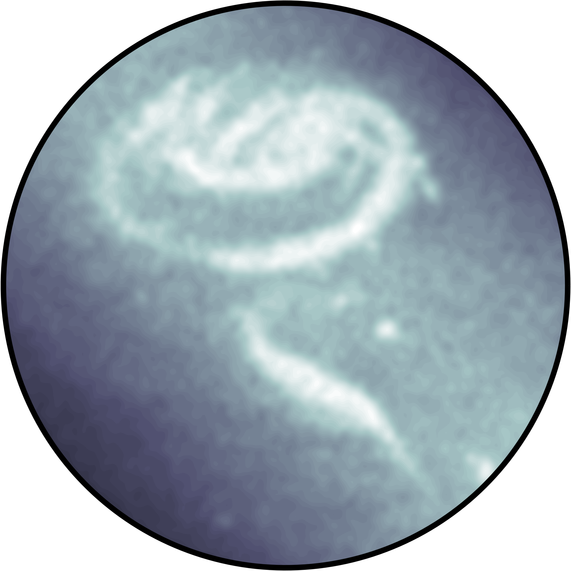
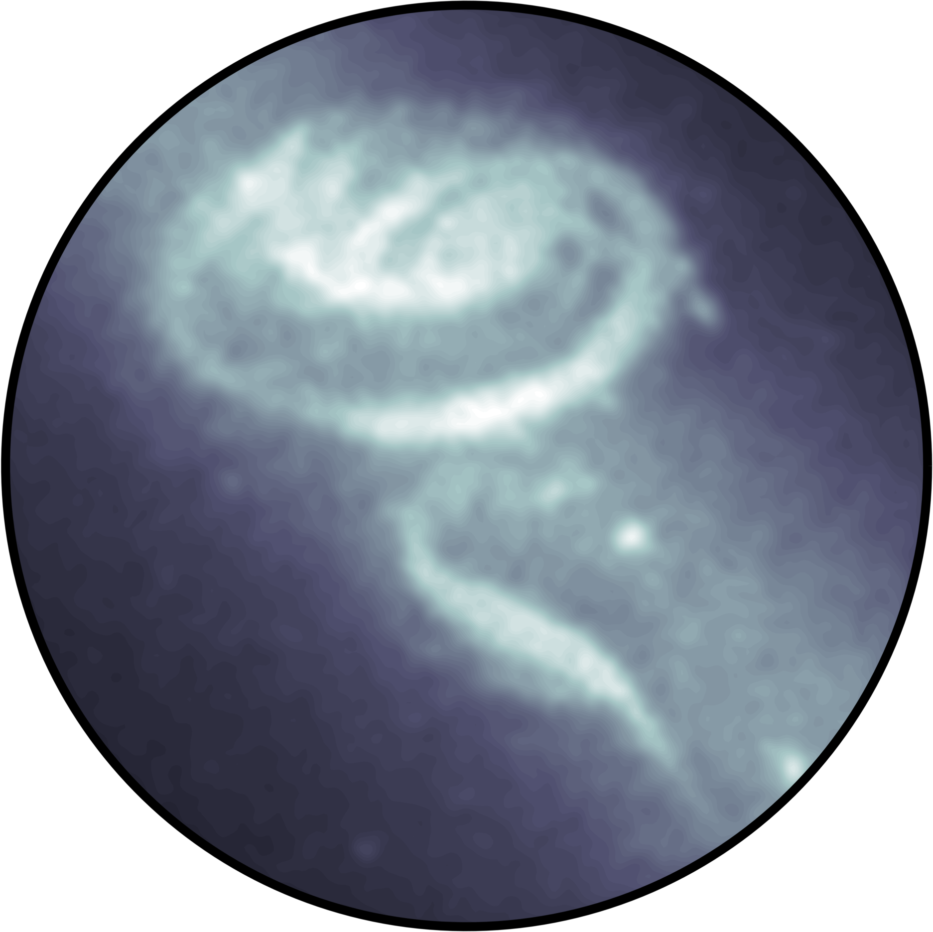
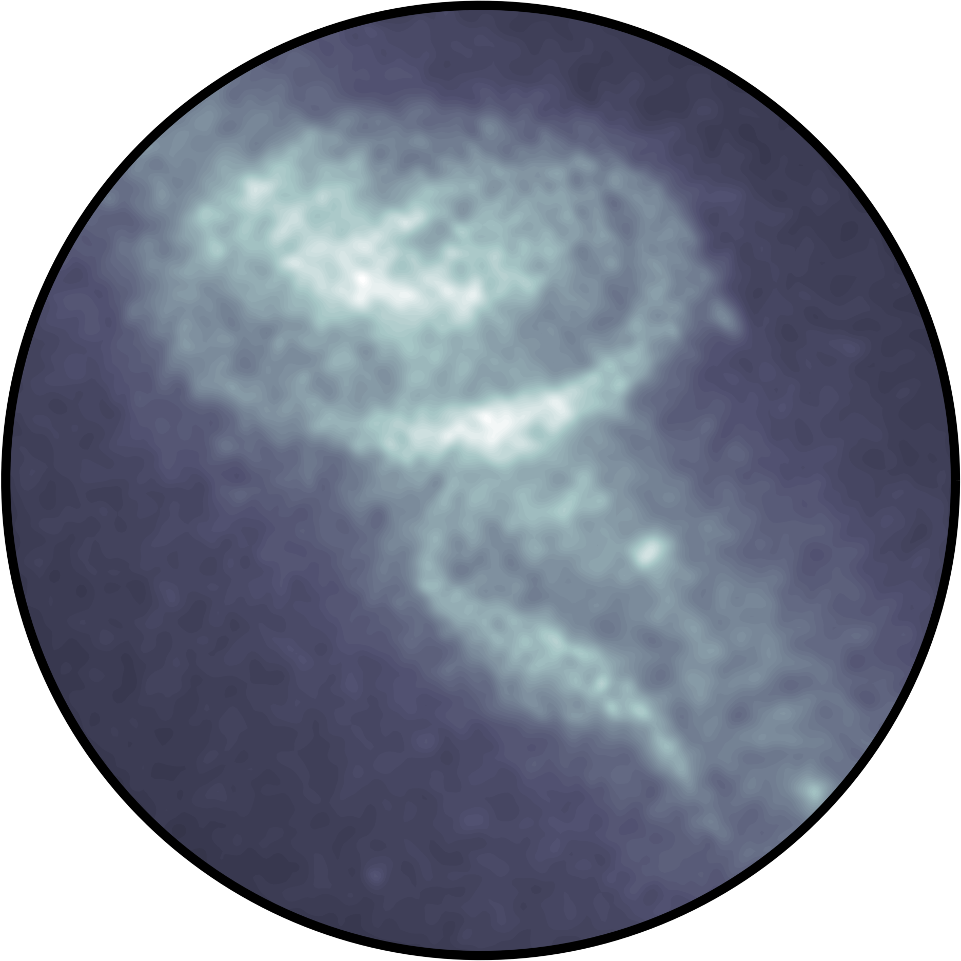
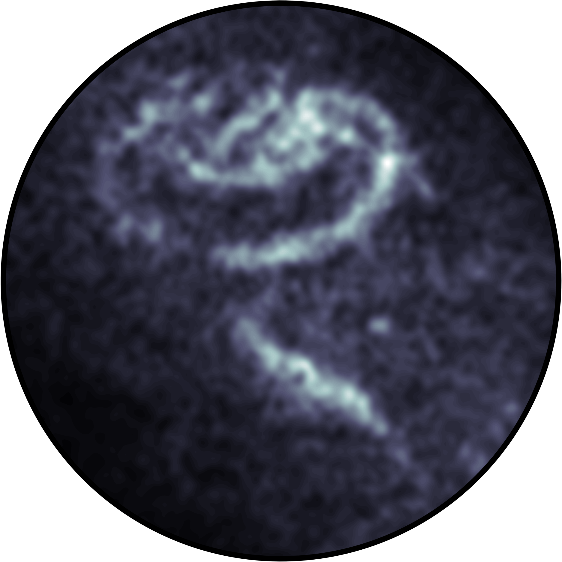
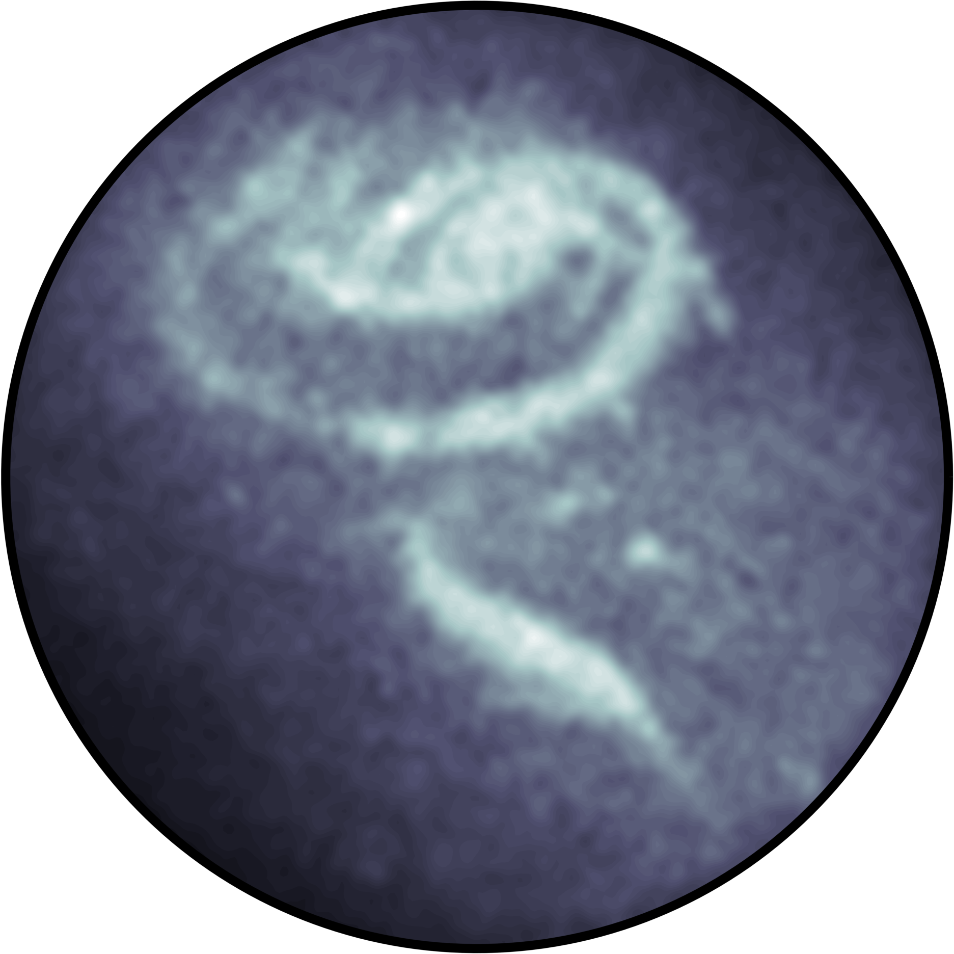
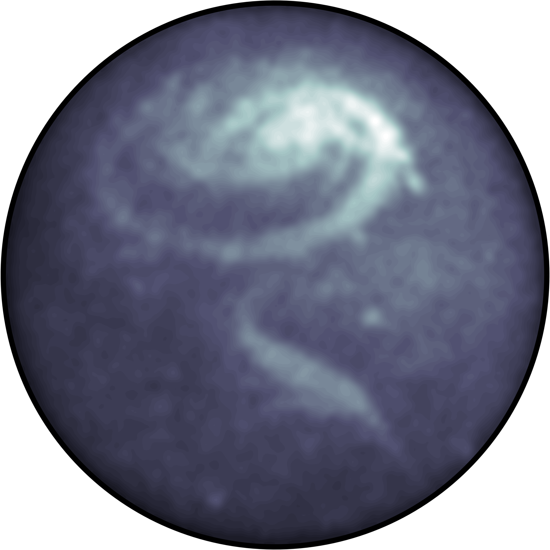
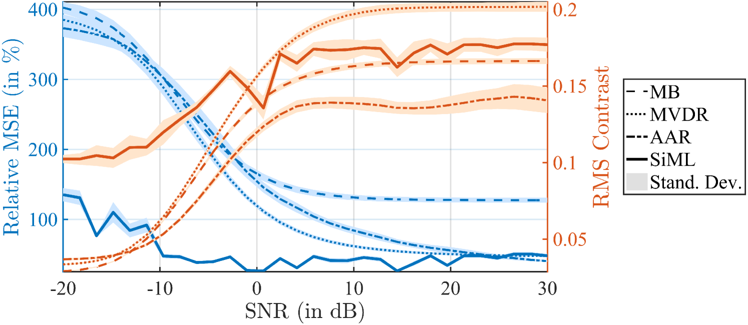
Fig. 2 compares the performance of the proposed Sieved Maximum Likelihood (SiML) method in a radio astronomy setup to three popular spectral-based methods, namely Matched Beamforming (MB), Maximum Variance Distortionless Response (MVDR) and the Adapted Angular Response (AAR) [34]. For this experiment, we generated randomly a layout antennas and simulated random measurements from the ground truth intensity field Fig. 2a. Furthermore, we considered two metrics to assess the quality of the recovered images: the traditional relative Mean Squared Error (MSE) and the Root Mean Squared (RMS) metric, which measures the contrast of an image by computing its standard deviation over all pixels. The simulations reveal that the SiML outperforms all the traditional algorithms for the considered SNR range in both metrics, except for large SNRs where MVDR exhibits a slightly better contrast. As for the traditional SML method, SiML performs particularly well for challenging scenarios with very low SNR.
4 Conclusion
SiML generalises the traditional SML method to a wider class of signals, encompassing arbitrarily shaped, possibly correlated, sources of which there may be more than the number of sensors. The method is numerically stable and admits a nice geometrical interpretation in the case of known noise power. Simulations revealed its superiority with respect to state-of-the-art subspace-based methods, both in terms of accuracy and contrast. Finally, the tensor product structure in Eq. 10 makes the estimate very efficient to compute. This is in contrast to traditional SML, which requires minimising a highly non-linear multi-dimensional function [1].
ß


References
- [1] Hamid Krim and Mats Viberg, “Two decades of array signal processing research: the parametric approach,” IEEE Signal processing magazine, vol. 13, no. 4, pp. 67–94, 1996.
- [2] Robert J Mailloux, Phased array antenna handbook, vol. 2, Artech House Boston, 2005.
- [3] Don H Johnson and Dan E Dudgeon, Array signal processing: concepts and techniques, Simon & Schuster, 1992.
- [4] Michael Brandstein and Darren Ward, Microphone arrays: signal processing techniques and applications, Springer Science & Business Media, 2013.
- [5] Jacob Benesty, Jingdong Chen, and Yiteng Huang, Microphone array signal processing, vol. 1, Springer Science & Business Media, 2008.
- [6] A Richard Thompson, James M Moran, and George W Swenson Jr, Interferometry and synthesis in radio astronomy, John Wiley & Sons, 2008.
- [7] Matthieu Simeoni, “Towards more accurate and efficient beamformed radio interferometry imaging,” M.S. thesis, EPFL, Spring 2015.
- [8] Simon Haykin, “Array signal processing,” Englewood Cliffs, NJ, Prentice-Hall, Inc., 1985, 493 p. For individual items see A85-43961 to A85-43963., vol. 1, 1985.
- [9] Lal Chand Godara, “Application of antenna arrays to mobile communications. ii. beam-forming and direction-of-arrival considerations,” Proceedings of the IEEE, vol. 85, no. 8, pp. 1195–1245, 1997.
- [10] Arogyaswami J Paulraj and Constantinos B Papadias, “Space-time processing for wireless communications,” IEEE Signal Processing Magazine, vol. 14, no. 6, pp. 49–83, 1997.
- [11] P. Hurley and M. Simeoni, “Flexibeam: analytic spatial filtering by beamforming,” in International Conference on Acoustics, Speech and Signal Processing (ICASSP), IEEE, March 2016.
- [12] Zhi-Pei Liang and Paul C Lauterbur, Principles of magnetic resonance imaging: a signal processing perspective, The Institute of Electrical and Electronics Engineers Press, 2000.
- [13] Boaz Rafaely, Fundamentals of spherical array processing, vol. 8, Springer, 2015.
- [14] Petre Stoica, Björn Ottersten, Mats Viberg, and Randolph L Moses, “Maximum likelihood array processing for stochastic coherent sources,” IEEE Transactions on Signal Processing, vol. 44, no. 1, pp. 96–105, 1996.
- [15] Petre Stoica, Erik G Larsson, and Alex B Gershman, “The stochastic crb for array processing: A textbook derivation,” IEEE Signal Processing Letters, vol. 8, no. 5, pp. 148–150, 2001.
- [16] Petre Stoica and Arye Nehorai, “On the concentrated stochastic likelihood function in array signal processing,” Circuits, Systems and Signal Processing, vol. 14, no. 5, pp. 669–674, 1995.
- [17] MP Van Haarlem, MW Wise, AW Gunst, George Heald, JP McKean, JWT Hessels, AG De Bruyn, Ronald Nijboer, John Swinbank, Richard Fallows, et al., “Lofar: The low-frequency array,” Astronomy & Astrophysics, vol. 556, pp. A2, 2013.
- [18] Peter E Dewdney, Peter J Hall, Richard T Schilizzi, and T Joseph LW Lazio, “The square kilometre array,” Proceedings of the IEEE, vol. 97, no. 8, pp. 1482–1496, 2009.
- [19] Martin Vetterli, Jelena Kovačević, and Vivek K Goyal, Foundations of signal processing, Cambridge University Press, 2014.
- [20] James O Ramsay, Functional data analysis, Wiley Online Library, 2006.
- [21] Mikhail Lifshits, “Lectures on gaussian processes,” in Lectures on Gaussian Processes, pp. 1–117. Springer, 2012.
- [22] Ulf Grenander and Grenander Ulf, “Abstract inference,” Tech. Rep., 1981.
- [23] Stuart Geman and Chii-Ruey Hwang, “Nonparametric maximum likelihood estimation by the method of sieves,” The Annals of Statistics, pp. 401–414, 1982.
- [24] Harish S Bhat and Nitesh Kumar, “On the derivation of the bayesian information criterion,” School of Natural Sciences, University of California, 2010.
- [25] James O Ramsay and Bernard W Silverman, Applied functional data analysis: methods and case studies, vol. 77, Citeseer, 2002.
- [26] Björn Ottersten, Peter Stoica, and Richard Roy, “Covariance matching estimation techniques for array signal processing applications,” Digital Signal Processing, vol. 8, no. 3, pp. 185–210, 1998.
- [27] Nathaniel R Goodman, “Statistical analysis based on a certain multivariate complex gaussian distribution (an introduction),” The Annals of mathematical statistics, vol. 34, no. 1, pp. 152–177, 1963.
- [28] Robert G Gallager, Principles of digital communication, vol. 1, Cambridge University Press Cambridge, UK:, 2008.
- [29] T Douglas Mast, “Fresnel approximations for acoustic fields of rectangularly symmetric sources,” The Journal of the Acoustical Society of America, vol. 121, no. 6, pp. 3311–3322, 2007.
- [30] KG Jinadasa, “Applications of the matrix operators vech and vec,” Linear Algebra and its Applications, vol. 101, pp. 73–79, 1988.
- [31] D Maiwald and D Kraus, “Calculation of moments of complex wishart and complex inverse wishart distributed matrices,” IEE Proceedings-Radar, Sonar and Navigation, vol. 147, no. 4, pp. 162–168, 2000.
- [32] Victor M Panaretos, “Statistics for mathematicians,” .
- [33] Heinz Werner Engl, Martin Hanke, and Andreas Neubauer, Regularization of inverse problems, vol. 375, Springer Science & Business Media, 1996.
- [34] Alle-Jan van der Veen and Stefan J Wijnholds, “Signal processing tools for radio astronomy,” in Handbook of Signal Processing Systems, pp. 421–463. Springer, 2013.