This paper was converted on www.awesomepapers.org from LaTeX by an anonymous user.
Want to know more? Visit the Converter page.

Simple and high-precision Hamiltonian simulation by compensating Trotter error with linear combination of unitary operations

Pei Zeng peizeng@uchicago.edu Pritzker School of Molecular Engineering, The University of Chicago, Illinois 60637, USA    Jinzhao Sun jinzhao.sun.phys@gmail.com Clarendon Laboratory, University of Oxford, Parks Road, Oxford OX1 3PU, United Kingdom Blackett Laboratory, Imperial College London, London SW7 2AZ, United Kingdom    Liang Jiang liang.jiang@uchicago.edu Pritzker School of Molecular Engineering, The University of Chicago, Illinois 60637, USA    Qi Zhao zhaoqi@cs.hku.hk QICI Quantum Information and Computation Initiative, Department of Computer Science, Department of Computer Science, The University of Hong Kong, Pokfulam Road, Hong Kong
(September 30, 2025)
Abstract

Trotter and linear-combination-of-unitary (LCU) are two popular Hamiltonian simulation methods. The Trotter method is easy to implement and enjoys good system-size dependence endowed by commutator scaling, while the LCU method admits high accuracy simulation with a smaller gate cost. We propose Hamiltonian simulation algorithms using LCU to compensate Trotter error, which enjoy both of their advantages. By adding few gates after the KKth-order Trotter formula, we realize a better time scaling than 2KKth-order Trotter. Our first algorithm exponentially improves the accuracy scaling of the KKth-order Trotter formula. For a generic Hamiltonian, the estimated gate counts of the first algorithm can be 2 orders of magnitude smaller than the best analytical bound of fourth-order Trotter formula. In the second algorithm, we consider the detailed structure of Hamiltonians and construct LCU for Trotter errors with commutator scaling. Consequently, for lattice Hamiltonians, the algorithm enjoys almost linear system-size dependence and quadratically improves the accuracy of the KKth-order Trotter. For the lattice system, the second algorithm can achieve 3 to 4 orders of magnitude higher accuracy with the same gate costs as the optimal Trotter algorithm. These algorithms provide an easy-to-implement approach to achieve a low-cost and high-precision Hamiltonian simulation.

I INTRODUCTION

Hamiltonian simulation, i.e., to simulate the real-time evolution U(t)=eiHtU(t)=e^{-iHt} of a physical Hamiltonian H=lHlH=\sum_{l}H_{l}, is considered to be a natural and powerful application of quantum computing Feynman (1982). It can also be used as an important subroutine in many other quantum algorithms like ground-state preparation Abrams and Lloyd (1999); Aspuru-Guzik et al. (2005), optimization problems Farhi et al. (2014); Zhou et al. (2020), and quantum linear solvers Harrow et al. (2009). To pursue real-world applications of Hamiltonian simulation with near-term quantum devices, we need to design feasible algorithms with small space complexity (i.e., qubit number) and time complexity (i.e., circuit depth and gate number).

One of the most natural Hamiltonian simulation methods is based on Trotter formulas Lloyd (1996); Suzuki (1990, 1991); Berry et al. (2007); Campbell (2019); Childs et al. (2019); Childs and Su (2019); Endo et al. (2019); Heyl et al. (2019); Chen et al. (2021); Şahinoğlu and Somma (2021); Su et al. (2021); Tran et al. (2020); Childs et al. (2021); Layden (2021); Zhao et al. (2022), which approximate the real-time evolution of H=l=1LHlH=\sum_{l=1}^{L}H_{l} by the product of the simple evolution of its summands eiHlte^{-iH_{l}t}. Besides its prominent advantage of simple realization without ancillas, Trotter methods are recently rigorously shown to enjoy commutator scaling Childs and Su (2019); Childs et al. (2021), i.e., the Trotter error is only related to the nested commutators of the Hamiltonian summands {Hl}\{H_{l}\}. This is very helpful for the Hamiltonians with strong locality constraints. For example, when we consider nn-qubit lattice Hamiltonians, the gate cost of high-order Trotter methods is almost linear to the system size nn, which is nearly optimal Childs and Su (2019). The major drawback of the Trotter methods is its polynomial gate cost to the inversed accuracy 1/ε1/\varepsilon, Poly(1/ε)\rm Poly(1/\varepsilon). This is unfavorable in many applications where high-precision simulation is demanded to obtain practical advantages over the existing classical algorithms Reiher et al. (2017).

In recent years, we have seen the developments of “post-Trotter” algorithms with exponentially improved accuracy dependence Berry et al. (2014, 2015, 2015); Low and Chuang (2019, 2017); Low (2019). Due to the smart choice of the expansion formulas (i.e., Taylor series Berry et al. (2015) or Jacobi-Anger expansion Low and Chuang (2017)), these post-Trotter methods are able to catch the dominant terms in the time evolution operator U(t)U(t) with polynomially increasing gate resources, leading to a logarithmic gate-number dependence on the accuracy requirement 1/ε1/\varepsilon. Unlike Trotter methods, these advanced algorithms are not able to utilize the specific structure of Hamiltonians due to the lack of commutator-based error form. Consequently, for instance, for nn-qubit lattice Hamiltonians, their gate complexities are 𝒪(n2)\mathcal{O}(n^{2}), which is worse than those in Trotter algorithms 𝒪(n1+o(1))\mathcal{O}(n^{1+o(1)}). Furthermore, these post-Trotter algorithms require the implementation of linear combination of unitary (LCU) formulas Childs and Wiebe (2012); Long (2011) or block encoding of Hamiltonians Low and Chuang (2019) which often costs many ancillary qubits and multicontrolled Toffoli gates. This is still experimentally challenging in a near-term or early fault-tolerant quantum computer Lin and Tong (2022). To reduce the hardware requirement of compiling the LCU formulas, recent studies focus on a random-sampling implementation of a LCU formula Childs and Wiebe (2012); Yang et al. (2021); Wan et al. (2022); Faehrmann et al. (2022), where the elementary unitaries are sampled to realize the LCU formula statistically. In this case, the Hamiltonian simulation is not performed by coherently implementing the unitary U=eiHtU=e^{-iHt}, but is instead realized through random sampling. This method remains effective for common applications, such as estimating the properties of the final state. Similar ideas have also been studied in the ground-state preparation algorithms Lin and Tong (2020); Zeng et al. (2021); Zhang et al. (2022).

Here, we propose composite algorithms that combine the inherent advantages of Trotter and LCU methods—easy implementation, high precision, and commutator scaling—by performing the Trotter method and then compensating the Trotter error with the LCU formulas we construct. We primarily focus on the random-sampling implementation of the LCU formula Childs and Wiebe (2012); Yang et al. (2021); Wan et al. (2022); Faehrmann et al. (2022), with the goal of estimating the properties of the target state after real-time evolution. We demonstrate that optimal performance can be achieved by allowing the Trotter circuit to handle the majority of the simulation, with the LCU method completing the remainder.

In Sec. II, we provide a summary of our construction and results, aimed at a general audience. We explain the key ideas behind the constructions with intuitive examples. For readers interested in the technical aspects, we introduce the necessary preliminary knowledge of Hamiltonian simulation in Sec. III to facilitate understanding of the technical results. Next, in Sec. IV and Sec. V, we present a detailed construction and gate complexity analysis of the two Trotter-LCU algorithms. Finally, in Sec. VI, we conclude our discussion and outline possible future directions.

II SUMMARY of RESULTS

II.1 General idea

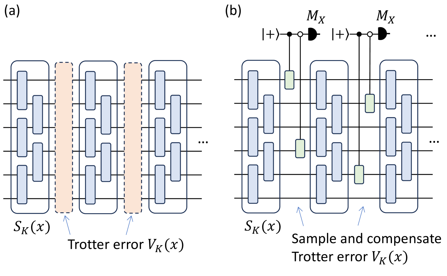
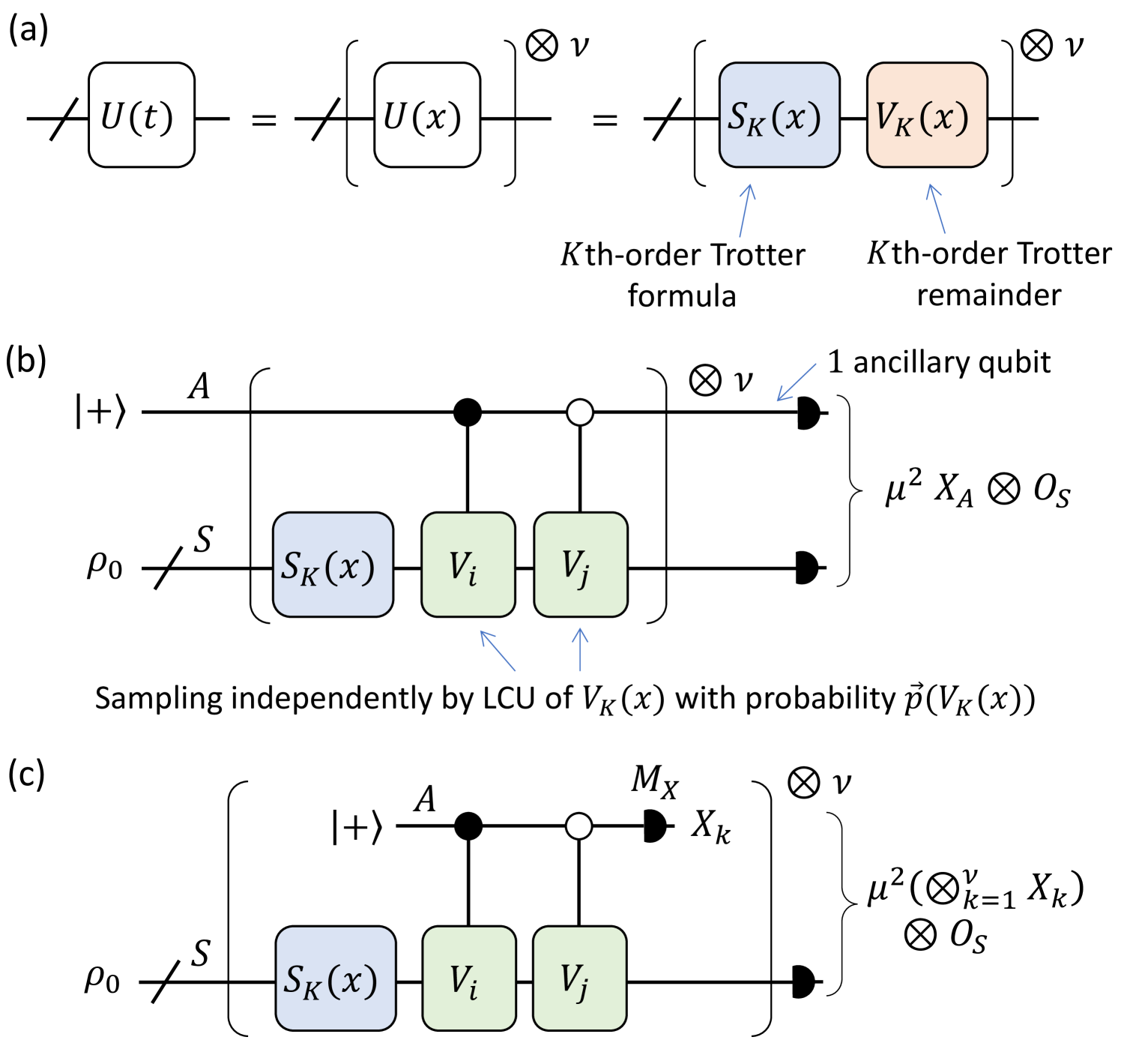
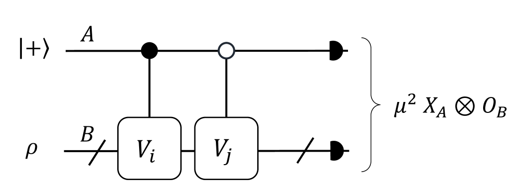
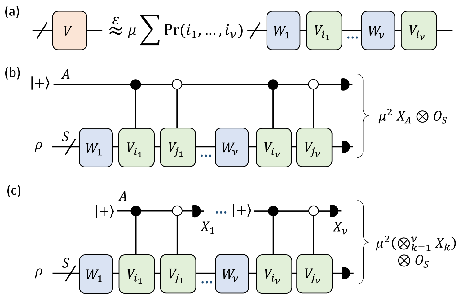
The major idea of the proposed Trotter-LCU algorithm is illustrated in Fig. 1. In a normal KKth-order Trotter circuit, we decompose the time evolution U(t)=eiHtU(t)=e^{-iHt} to ν\nu segments, each with a small evolution time x=t/νx=t/\nu. For consistency, we denote the 0th-order Trotter formula as S0(x)=IS_{0}(x)=I. After we perform the KKth-order Trotter formula SK(x)(K=0,1,2k,k+)S_{K}(x)(K=0,1,2k,k\in\mathbb{N}_{+}), there will be a remaining Trotter error VK(x):=U(x)SK(x)V_{K}(x):=U(x)S_{K}(x)^{\dagger}, which affects the simulation accuracy. To address this problem, we introduce a random LCU formula to compensate the Trotter error using one ancilla and simple gates, which achieves a high-precision Hamiltonian simulation with low cost.

Refer to caption
Figure 1: (a) In the normal KKth-order Trotter circuit, there will be a remaining Trotter error VK(x)V_{K}(x) after each segment. (b) We introduce random LCU formulas to compensate VK(x)V_{K}(x) with a single ancilla qubit and simple gates.

Consider the following LCU formula of an operator VV,

V~=μi=0Γ1Pr(i)Vi,\tilde{V}=\mu\sum_{i=0}^{\Gamma-1}\Pr(i)V_{i}, (1)

such that the spectral norm distance VV~ε\|V-\tilde{V}\|\leq\varepsilon. Here, μ>0\mu>0 is the 11-norm (i.e., l1l_{1}-norm) of the coefficient vector, Pr(i)\Pr(i) is a probability distribution over different unitaries ViV_{i}, and {Vi}i=0Γ1\{V_{i}\}_{i=0}^{\Gamma-1} is a set of unitaries. There are usually two ways to implement the LCU formula: the coherent implementation Berry et al. (2014, 2015) and the random-sampling implementation Yang et al. (2021); Wan et al. (2022); Faehrmann et al. (2022). Our major focus is on the random-sampling implementation, where we can estimate the properties of the target state ρ=U(t)ρ0U(t)\rho=U(t)\rho_{0}U(t)^{\dagger} with only one ancillary qubit. In Appendix H, we discuss the potential use of the coherent implementation of our algorithm. In the random-sampling implementation, we can use Eq. 1 to estimate an arbitrary observable value OO on ρ\rho,

Tr(Oρ)μ2i,jpipjTr(OViρ0Vj).\mathrm{Tr}(O\rho)\approx\mu^{2}\sum_{i,j}p_{i}p_{j}\mathrm{Tr}(OV_{i}\rho_{0}V_{j}^{\dagger}). (2)

As is shown in Fig. 2(b), since the estimation of Tr(OViρ0Vj)\mathrm{Tr}(OV_{i}\rho_{0}V_{j}^{\dagger}) can be implemented using Hadamard-test-type circuits Kitaev (1995), we only need to sample ViV_{i} and VjV_{j} based on the LCU formula in Eq. 1 to estimate Tr(Oρ)\mathrm{Tr}(O\rho) with ε\varepsilon accuracy using missingO(μ4/ε2)\mathcal{\mathcal{missing}}{O}(\mu^{4}/\varepsilon^{2}) sampling resource, which owns an extra μ4\mu^{4} overhead compared to the normal Hamiltonian simulation algorithms Faehrmann et al. (2022). To make the algorithm efficient, we need to set μ\mu to be a constant. We also provide a variant in Fig. 2(c) where the ancillary qubit is measured and reset in each segment, which is equivalent to Fig. 2(b) for the observable estimation. In this case, the expectation value of μ2XA(tot)OS\mu^{2}X^{(tot)}_{A}\otimes O_{S} provides an unbiased estimation of Tr(Oρ)\mathrm{Tr}(O\rho) where X(tot):=k=1νXkX^{(tot)}:=\bigotimes_{k=1}^{\nu}X_{k} is the multiplication of all the ancillary measurement values. This variant reduces the need to store the ancilla qubit, simplifying the implementation on a fault-tolerant quantum computer.

Refer to caption
Figure 2: (a) In the KKth-order Trotter-LCU algorithm, we first implement KKth-order Trotter formula, then compensate the remainder using the LCU formulas we construct. (b) Random-sampling implementation of the LCU formula. We sample the elementary unitaries ViV_{i} and VjV_{j} independently based on the LCU formula of VK(x)V_{K}(x) and implement the controlled ViV_{i} and VjV_{j} gate. Then the Trotter remainder VK(x)V_{K}(x) can be compensated in a Hadamard-test type circuit. (c) A variant of the implementation where the ancillary qubit is measured and reset in each segment. The detailed sampling procedure of ViV_{i} and VjV_{j} is shown in Fig. 5 and Fig. 7.

The construction of an appropriate LCU formula for the KKth-order Trotter remainder, VK(x)V_{K}(x), is crucial for developing an efficient Hamiltonian simulation algorithm. In the following subsections, we briefly introduce two approaches for constructing the LCU formula for VK(x)V_{K}(x). The resulting composite Trotter-LCU algorithms are referred to as paired Taylor-series compensation (PTSC) and nested-commutator compensation (NCC), respectively. Detailed analysis and performance proofs for these two algorithms can be found in Sec. IV and Sec. V.

II.2 Paired Taylor-series compensation: overview

Without loss of generality, we focus on the case of an nn-qubit Hamiltonian HH, which can be written as

H=l=1LHl=l=1LαlPl=λl=1LplPl,H=\sum_{l=1}^{L}H_{l}=\sum_{l=1}^{L}\alpha_{l}P_{l}=\lambda\sum_{l=1}^{L}p_{l}P_{l}, (3)

where {Pl}l\{P_{l}\}_{l} are different nn-qubit Pauli operators. We set all the coefficients {αl}l\{\alpha_{l}\}_{l} to be positive and absorb the signs into Pauli operators {Pl}l\{P_{l}\}_{l}. λ:=lαl\lambda:=\sum_{l}\alpha_{l} is the l1l_{1}-norm of the Hamiltonian coefficient vector. We consider the Hamiltonians where λ\lambda increases polynomially with respect to nn.

Refer to caption
Figure 3: Illustration of the idea of paired Taylor-series compensation (PTSC) algorithm. We take the first-order algorithm as an example. (a) Taylor-series expansion of the small-time evolution U(x)U(x). The 11-norm is λ(U(x))=eλx=1+𝒪(λx)\lambda(U(x))=e^{\lambda x}=1+\mathcal{O}(\lambda x). The dominant term is contributed from the first-order expansion F0,1(x)F_{0,1}(x). (b) By introducing the first-order Trotter formula S1(x)S_{1}(x), the first-order expansion F1,1F_{1,1} in the Trotter remainder V1(x)V_{1}(x) becomes 0. As a result, the 11-norm of V1(x)V_{1}(x) is suppressed to 1+𝒪((λx)2)1+\mathcal{O}((\lambda x)^{2}), limited by the second-order expansion term F1,2(x)F_{1,2}(x). (c) By further noticing that F1,2F_{1,2} and F1,3F_{1,3} are anti-Hermitian, we introduce Euler’s formula in Eq. 7 to pair the leading-order terms to F1,0:=IF_{1,0}:=I. This will double the order of μx1\mu_{x}-1 and further suppress the 11-norm μ\mu of the overall evolution U(t)U(t).

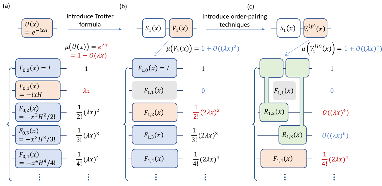
We first consider to construct the LCU formulas for VK(x)V_{K}(x) from Taylor-series expansion Berry et al. (2015). In the 0th-order case, when no Trotter formula is introduced, the Trotter remainder V0(x)V_{0}(x) is the short-time evolution U(x)U(x) itself, which can be expanded as

V0(x)\displaystyle V_{0}(x) =eixH=s=0F0,s(x)=s=0(ix)ss!Hs\displaystyle=e^{-ixH}=\sum_{s=0}^{\infty}F_{0,s}(x)=\sum_{s=0}^{\infty}\frac{(-ix)^{s}}{s!}H^{s} (4)
=eλxs=0Poi(s;λx)l1,,lspl1plsPl1Pls.\displaystyle=e^{\lambda x}\sum_{s=0}^{\infty}\mathrm{Poi}(s;\lambda x)\sum_{l_{1},...,l_{s}}p_{l_{1}}.p_{l_{s}}P_{l_{1}}.P_{l_{s}}.

Here, Poi(s;a):=eaas/s!\mathrm{Poi}(s;a):=e^{-a}a^{s}/s! is the Poisson distribution. F0,s(x)F_{0,s}(x) denotes the ss-order expansion term. Eq. 4 illustrated in Fig. 3(a) is a LCU formula of V0(x)V_{0}(x) with 11-norm μx=eλx\mu_{x}=e^{\lambda x}. The 11-norm of the overall evolution U(t)=U(x)νU(t)=U(x)^{\nu} is then μ=eλt\mu=e^{\lambda t}, which, unfortunately, grows exponentially with respect to tt regardless of how much we increase the segment number ν\nu. This implies that the direct random-sampling implementation of the LCU formula V0(x)V_{0}(x) in Eq. 4 is not feasible. In Ref. Berry et al. (2015), the authors discuss the coherent implementation of V0(x)V_{0}(x) instead and find that one can achieve good time and accuracy dependence in that scenario.

When focusing on the random-sampling implementation, we need to suppress the 11-norm μx\mu_{x} of each segment. To this end, we first consider the usage of the Trotter formula. For example, if we apply first-order Trotter formula S1(x)=l=1LeixHlS_{1}(x)=\prod_{l=1}^{L}e^{-ixH_{l}} in each segment, the first-order remainder V1(x):=U(x)S1(x)V_{1}(x):=U(x)S_{1}(x)^{\dagger} can be expanded as

V1(x)\displaystyle V_{1}(x) =eixHl=L1eixHl=s=0F1,s(x)\displaystyle=e^{-ixH}\prod_{l=L}^{1}e^{ixH_{l}}=\sum_{s=0}^{\infty}F_{1,s}(x) (5)
=r;r1,r2,,rL(ix)rr!Hrl=L1(ix)rlrl!Hrl,\displaystyle=\sum_{r;r_{1},r_{2},...,r_{L}}\frac{(-ix)^{r}}{r!}H^{r}\prod_{l=L}^{1}\frac{(ix)^{r_{l}}}{r_{l}!}H^{r_{l}},

where {r1,,rL}\{r_{1},...,r_{L}\} denotes LL expansion variables related to the Trotter formula and s:=r+l=1Lrls:=r+\sum_{l=1}^{L}r_{l}. F1,sF_{1,s} denotes the ss-order expansion term of V1(x)V_{1}(x). The 11-norm of V1(x)V_{1}(x) in Eq. 5 is e2λxe^{2\lambda x}, which seems to be even larger than the 0th-order case. However, since V1(x)V_{1}(x) denotes the (multiplicative) Trotter error, we have F1,1(x)=0F_{1,1}(x)=0. Using this condition, we can rewrite V1(x)V_{1}(x) as

V1(x)=I+s=2F1,s(x),V_{1}(x)=I+\sum_{s=2}^{\infty}F_{1,s}(x), (6)

as illustrated in Fig. 3. From the Taylor-series expansion, we can bound the 11-norm of the new LCU formula in Eq. 6 by μx=e2λx(2λx)e(2λx)2\mu_{x}=e^{2\lambda x}-(2\lambda x)\leq e^{(2\lambda x)^{2}}. In this way, we reduce μx\mu_{x} from 1+𝒪(λx)1+\mathcal{O}(\lambda x) to 1+𝒪((λx)2)1+\mathcal{O}((\lambda x)^{2}). The 11-norm of the overall time evolution becomes μ=μxνexp((2λt)2/ν)\mu=\mu_{x}^{\nu}\leq\exp((2\lambda t)^{2}/\nu). As a result, by increasing the segment number ν\nu — or equivalently reducing the unit evolution time xx — we can decrease the 1-norm μ\mu, leading to a lower sampling cost. If we choose the segment number as ν=𝒪((λt)2)\nu=\mathcal{O}((\lambda t)^{2}), μ\mu will remain constant.

From the above discussion, it is clear that, to reduce the 1-norm μ\mu of the overall LCU formula for U=eiHtU=e^{-iHt}, our main objective is to suppress the leading-order term of the 11-norm remainder μx1\mu_{x}-1 for each segment, which determines the number of segments ν\nu and hence circuit depth when μ\mu is set to be a constant.

We can further reduce the 11-norm μx\mu_{x} of V1(x)V_{1}(x) by taking advantage of the structure of Trotter errors. For an anti-Hermian Pauli operator ±iP\pm iP where P{I,X,Y,Z}nP\in\{I,X,Y,Z\}^{\otimes n}, we have the following Euler’s formula,

I±iyP=1+y2e±iθP.I\pm iyP=\sqrt{1+y^{2}}e^{\pm i\theta P}. (7)

Here, θ=tan1(y)\theta=\tan^{-1}(y) and we suppose 0<y<10<y<1. The 1-norm of the left-hand side of Eq. 7 is 1+y1+y, while the 1-norm of the right-hand side is 1+y2<1+y22=1+𝒪(y2)\sqrt{1+y^{2}}<1+\frac{y^{2}}{2}=1+\mathcal{O}(y^{2}). As a result, the exponent of μx1\mu_{x}-1 is effectively doubled. In subsection IV.2, we prove that the expansion terms F1,2F_{1,2} and F1,3F_{1,3} in the LCU formula Eq. 5 are anti-Hermitian. As a result, we can further suppress μx\mu_{x} by pairing the terms in F1,s(x)F_{1,s}(x) with F1,0=IF_{1,0}=I using Euler’s formula in Eq. 7. When y=xsy=x^{s}, the paired formula R1,s(x)R_{1,s}(x) as a summation of Pauli rotation unitaries owns the 11-norm of μx=1+𝒪(x2s)\mu_{x}=1+\mathcal{O}(x^{2s}), whose xx dependence is doubled, as illustrated inFig. 3(c).

To generalize the discussion, for the KKth-order Trotter error VK(x)V_{K}(x) (K=2kK=2k, k+k\in\mathbb{N}_{+}), we have FK,1=FK,K=0F_{K,1}=...F_{K,K}=0 Suzuki (1990); Childs et al. (2021). Moreover, we can show that FK,K+1F_{K,K+1}, FK,K+2F_{K,K+2},…, FK,2K+1F_{K,2K+1} are anti-Hermitian. We call the term with s=K+1s=K+1 to 2K+12K+1 the leading-order terms. The algorithm utilizing KKth-order Trotter formula and the paired idea in the LCU construction is called the KKth-order PTSC algorithm. We provide the detailed algorithm description and gate-complexity analysis in Sec. IV.

The PTSC algorithm is generic for the LL-sparse Hamiltonian H=l=1LHl=λl=1LplPlH=\sum_{l=1}^{L}H_{l}=\lambda\sum_{l=1}^{L}p_{l}P_{l} with λ=lHl\lambda=\sum_{l}\|H_{l}\| and {Pl}\{P_{l}\} are Pauli matrices. It can be implemented using a simple and universal classical random-sampling procedure: first, we sample the order ss from the Taylor-series expansion, and then we sample a Pauli string based on the Hamiltonian coefficients. With the random-sampling implementation, we prove that by appending few gates after the KKth-order Trotter formula with only one ancillary qubit, one can improve the time scaling from 1+1/K1+1/K to 1+1/(2K+1)1+1/(2K+1) and exponentially improves the accuracy scaling of the KKth-order Trotter formula compared to the KKth-order Trotter. We have the following theorem.

Theorem 1 (Informal, see Theorem 1 in Sec. IV) In a KKth-order paired Taylor-series compensation algorithm (K=0,1K=0,1 or 2k2k, k+k\in\mathbb{N}_{+}), the gate complexity in a single round is 𝒪((λt)1+12K+1(κKL+log(1/ε)loglog(1/ε)))\mathcal{O}\left((\lambda t)^{1+\frac{1}{2K+1}}(\kappa_{K}L+\frac{\log(1/\varepsilon)}{\log\log(1/\varepsilon)})\right), where λ=lHl\lambda=\sum_{l}\|H_{l}\|, κK=K\kappa_{K}=K when K=0K=0 or 11, κK=2×5K/21\kappa_{K}=2\times 5^{K/2-1} otherwise.

From Theorem 1, we observe that setting K=0K=0, i.e., not using Trotter formulas, still yields a valid PTSC algorithm by pairing F0,1F_{0,1} with II. In this case, the gate complexity is independent of the sparsity LL but quadratically dependent on tt, similar to the algorithm in Ref. Wan et al. (2022). Conversely, when using a KKth-order Trotter formula, the PTSC algorithm becomes LL dependent with an almost linear dependence on tt. In both cases, the PTSC algorithms achieve high simulation accuracy ε\varepsilon. We expect the 0th-order algorithm to be particularly useful for quantum chemistry Hamiltonians with large LL, while higher-order algorithms are better suited for generic LL-sparse Hamiltonians with long simulation times tt.

II.3 Nested-commutator compensation: overview

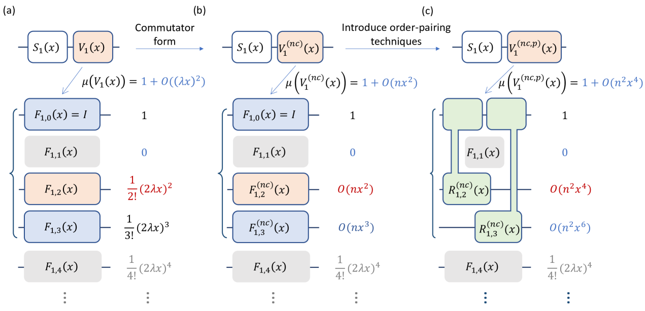
The PTSC algorithms above are generic and applicable to any Hamiltonian. When we consider the detailed structure of Hamiltonians, we could make the compensation algorithms more efficient by taking advantage of the commutation relationship of the terms in the Hamiltonians, which was formerly also studied in the Trotter algorithms Childs et al. (2021).

We will take the first-order Trotter remainder V1(x)V_{1}(x) as an illustrative example. Following the Taylor-series expansion in Eq. 5, the second-order term F1,2(x)F_{1,2}(x) in V1(x)V_{1}(x) can be written as

F1,2(x)\displaystyle F_{1,2}(x) =r;rr+r=2(ixH)rr!l=L1(ixHl)rlrl!.\displaystyle=\sum_{\begin{subarray}{c}r;\vec{r}\\ r+\sum\vec{r}=2\end{subarray}}\frac{(-ixH)^{r}}{r!}\prod_{l=L}^{1}\frac{(ixH_{l})^{r_{l}}}{r_{l}!}. (8)

Since F1,2(x)F_{1,2}(x) is anti-Hermitian, all the Hermitian expansion terms in Eq. 8 will cancel out. We can then simplify F1,2(x)F_{1,2}(x) as,

F1,2(x)\displaystyle F_{1,2}(x) =(ix)2(l=1LHl22!+l,l:l>lHlHl)\displaystyle=(ix)^{2}\left(\sum_{l=1}^{L}\frac{H_{l}^{2}}{2!}+\sum_{l,l^{\prime}:l>l^{\prime}}H_{l}H_{l^{\prime}}\right) (9)
+(ixH)l=1L(ixHl)+(ixH)22!\displaystyle\quad+(-ixH)\sum_{l=1}^{L}(ixH_{l})+\frac{(-ixH)^{2}}{2!}
=x22l,l:l>l[Hl,Hl],\displaystyle=\frac{x^{2}}{2}\sum_{l,l^{\prime}:l>l^{\prime}}[H_{l^{\prime}},H_{l}],

which is a summation of L(L1)L(L-1) commutators. Since the commutators of Hermitian operators are always anti-Hermitian, this implies that the nested-commutator expansion of F1,2(x)F_{1,2}(x) in Eq. 9 is compact enough since there is no Hermitian expansion terms in it.

For a common physical Hamiltonian with locality constraints, we can take advantage of the commutator-form expression like Eq. 9. For example, for an nn-qubit lattice Hamiltonian with the form,

H=j=0n1Hj,j+1,H=\sum_{j=0}^{n-1}H_{j,j+1}, (10)

where the summand Hj,j+1H_{j,j+1} acts on the jjth and (j+1)(j+1)th vertices. We can split the Hamiltonian to two components H=A+BH=A+B where A:=j:evenHj,j+1,B:=j:oddHj,j+1A:=\sum_{j:\mathrm{even}}H_{j,j+1},\quad B:=\sum_{j:\mathrm{odd}}H_{j,j+1} , so that the summands Hj,j+1H_{j,j+1} commute with each other in each component. We denote the norm of each Hamiltonian summand as

Λ=maxjHj,j+1,Λ1\displaystyle\Lambda=\max_{j}\|H_{j,j+1}\|,\quad\Lambda_{1} =maxjHj,j+11.\displaystyle=\max_{j}\|H_{j,j+1}\|_{1}. (11)

Now, suppose we estimate the 11-norm of F1,2(x)F_{1,2}(x) of the lattice Hamiltonian based on Eq. 9, we can see that there are only nn nonzero terms: for any given Hamiltonian component Hj,j+1H_{j,j+1}, only Hji,jH_{j-i,j} and Hj+1,j+2H_{j+1,j+2} do not commute with it. Then, the norm of F1,2(x)F_{1,2}(x) is bounded by

F1,2(x)1nΛ1x22=𝒪(nx2).\|F_{1,2}(x)\|_{1}\leq n\Lambda_{1}\frac{x^{2}}{2}=\mathcal{O}(nx^{2}). (12)

Comparing with the original bound in Eq. 62, F1,2(x)1η2=𝒪((λx)2)=𝒪(n2x2)\|F_{1,2}(x)\|_{1}\leq\eta_{2}=\mathcal{O}((\lambda x)^{2})=\mathcal{O}(n^{2}x^{2}), we improve the system-size-related factor nn. The improved system-size nn dependence of the 1-norm F1,2(x)1\|F_{1,2}(x)\|_{1} suggests a corresponding improvement in the system-size dependence of the gate complexity for the nested commutator algorithm.

Refer to caption
Figure 4: Illustration of the idea of nested-commutator compensation (NCC) algorithm. We take the first-order algorithm K=1K=1 as an example. (a) The Taylor-series expansion of the first-order Trotter remainder. We consider a truncation such that the higher-order terms with order s2K+2s\geq 2K+2 will not be compensated. (b) We derive the nested-commutator form for the leading-order expansion terms F1,2(nc)(x)F_{1,2}^{(nc)}(x) and F1,3(nc)(x)F_{1,3}^{(nc)}(x), which own better system-size dependence. (c) Since F1,2(nc)F^{(nc)}_{1,2} and F1,3(nc)F^{(nc)}_{1,3} are anti-Hermitian, we introduce Euler’s formula in Eq. 7 to pair the leading-order terms to F1,0:=IF_{1,0}:=I. This will double the order of μx1\mu_{x}-1 and further suppress the 11-norm μ\mu of the overall evolution U(t)U(t).

Now, we are going to generalize the idea above. In Sec. V, we show how to expand the second- and third-order terms of V1(x)V_{1}(x) as a summation of nested commutators,

F1,s(x)\displaystyle F_{1,s}(x) =xss!Cs1=(ix)ss!(𝒜com(s1)(HL,,H1;H)\displaystyle=\frac{x^{s}}{s!}C_{s-1}=\frac{(-ix)^{s}}{s!}\Big{(}\mathcal{A}_{\mathrm{com}}^{(s-1)}(H_{L},.,H_{1};H) (13)
l=1L𝒜com(s1)(HL,,Hl+1;Hl)),s=2,3,\displaystyle\,-\sum_{l=1}^{L}\mathcal{A}_{\mathrm{com}}^{(s-1)}(H_{L},.,H_{l+1};H_{l})\Big{)},\quad s=2,3,

where 𝒜com(s)(AL,,A1;B)\mathcal{A}_{\mathrm{com}}^{(s)}(A_{L},...,A_{1};B) is defined to be

m1++mL=s(sm1,,mL)adALmLadA1m1B.\displaystyle\sum_{m_{1}+...+m_{L}=s}\binom{s}{m_{1},...,m_{L}}\mathrm{ad}_{A_{L}}^{m_{L}}.\mathrm{ad}_{A_{1}}^{m_{1}}B. (14)

We also use the adjoint notation adALadA1B:=[AL,[A1,B]]\mathrm{ad}_{A_{L}}...\mathrm{ad}_{A_{1}}B:=[A_{L},...[A_{1},B]...]. It is easy to check that the form of F1,s(x)F_{1,s}(x) (s=2s=2 or 33) in Eq. 13 is anti-Hermitian, which is consistent with the discussion in the paired Taylor-series algorithm in the previous section. We can also generalize the method to the case of KKth-order Trotter remainder, that is, to express the expansion terms FK,sF_{K,s} of the KKth-order Trotter remainder based on the nested commutators.

Based on the nested-commutator expansion, we propose the KKth-order nested-commutator compensation (NCC) algorithm. As is illustrated in Fig. 4, in the construction of NCC, we first utilize the nested-commutator forms of Trotter error terms from K+1K+1 to 2K+12K+1 order, i.e., the leading-order terms; then we apply the order-pairing techniques similar to PTSC in Fig. 3(c) to further suppress the 11-norm of μx\mu_{x}. A key difference between NCC and PTSC algorithms is that in PTSC algorithms, we compensate the Trotter error VK(x)V_{K}(x) up to arbitrary order; while in NCC algorithms, we only compensate VK(x)V_{K}(x) for leading-order terms, which shrinks the error from missingO(xK+1)\mathcal{\mathcal{missing}}{O}(x^{K+1}) to 𝒪(x2K+2)\mathcal{O}(x^{2K+2}) in one slice with the sampling cost μ=1+𝒪(CK1(K+1)!x2K+2)\mu=1+\mathcal{O}(\frac{\|C_{K}\|_{1}}{(K+1)!}x^{2K+2}). The gate complexity estimation is then converted to the calculation of the 11-norm of the commutator CK1\|C_{K}\|_{1}. For instance, if we consider the nn-qubit lattice Hamiltonian models in Eq. 10, then we can prove that CK1=𝒪(n)\|C_{K}\|_{1}=\mathcal{O}(n). We can then provide the following performance guarantee for the NCC algorithms.

Theorem 2 (Informal, see Theorem 2 in Sec. V) In a KKth-order nested-commutator compensation (NCC) algorithm (K=1K=1 or 2k2k) with nn-qubit lattice Hamiltonians, the gate complexity in a single round is 𝒪(n1+22K+1t1+12K+1ε12K+1)\mathcal{O}(n^{1+\frac{2}{2K+1}}t^{1+\frac{1}{2K+1}}\varepsilon^{-\frac{1}{2K+1}}).

Compared to the performance of KKth-order Trotter algorithm 𝒪((nt)1+1/Kε1/K)\mathcal{O}((nt)^{1+1/K}\varepsilon^{-1/K}) Childs and Su (2019), we achieve tt- and ε\varepsilon-dependence better than 2K2Kth-order Trotter using only KKth-order Trotter formula with simple compensation gates of Pauli-rotation operators. To generalize the result in Theorem 2, we also study the performance of Nested Commutator (NCC) algorithms when applied to a general Hamiltonian in subsection V.3.

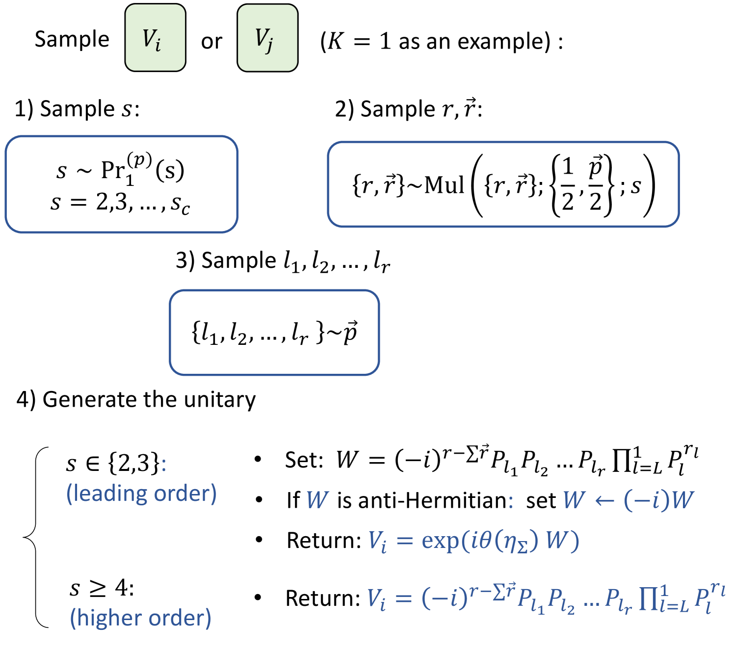
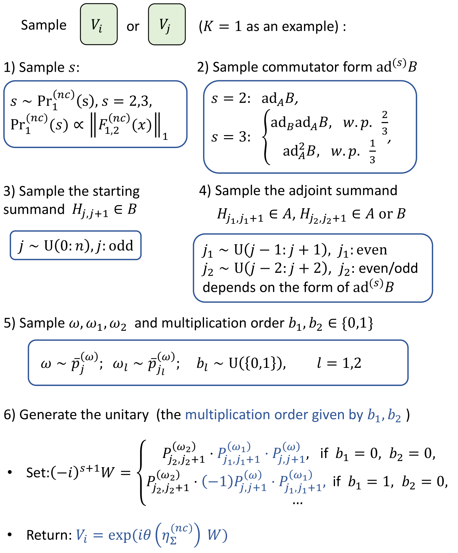
II.4 Efficient random-sampling implementation

A simple implementation of the Trotter-LCU algorithm in Fig. 2(b) or Fig. 2(c) requires not only an easy-to-implement quantum circuit but also efficient classical random sampling of Pauli operators from the Trotter remainder VK(x)V_{K}(x). We now briefly discuss how to realize an efficient classical random sampling in PTSC and NCC algorithms, that is, with a space resource of 𝒪(κKK)\mathcal{O}(\kappa_{K}K) and time resource of 𝒪(K(logL+logκK))\mathcal{O}(K(\log{L}+\log\kappa_{K})) where LL is the sparsity of the Hamiltonian.

A key idea for achieving efficient sampling is to use a multistage hierarchical sampling algorithm. Rather than fully expanding the Trotter remainder into a direct summation of Pauli operators, we structure the LCU formula into multiple layers. This allowss us to decompose the overall Pauli operator sampling process into a series of simpler, more manageable sampling tasks.

In the PTSC algorithm, the Trotter remainder in Eq. 5 is derived by expanding the time-evolution eixHe^{-ixH} and each Hamiltonian summand term eixHle^{ixH_{l}} by Taylor series independently. As a result, the sampling can be done by first sampling the overall expansion order ss, then sample the individual expansion order rr of Hamiltonian HH or the expansion order r:=[r1,r2,,rL]\vec{r}:=[r_{1},r_{2},...,r_{L}] of the summands {Hl}\{H_{l}\}. The sampling of rr and r\vec{r}, following the analysis in Sec. IV, can be done based on a multinomial distribution Mul(r,r;{12,p2};s)\text{Mul}(r,\vec{r};\{\frac{1}{2},\frac{\vec{p}}{2}\};s) where p:=[p1,p2,,pL]\vec{p}:=[p_{1},p_{2},...,p_{L}] denotes the normalized coefficient factor of HH defined in Eq. 3. For the sampled Hamiltonian HH, we further sample the summands HlH_{l} inside based on p\vec{p}. We summarize the sampling algorithm in Fig. 5.

Refer to caption
Figure 5: The sampling procedure of ViV_{i} or VjV_{j} in Fig. 2(b,c) in the PTSC algorithm. We set K=1K=1 as example. Pr1(p)(s)\Pr_{1}^{(p)}(s) is a discrete probability distribution given in Eq. 77. ηΣ:=η2+η3\eta_{\Sigma}:=\eta_{2}+\eta_{3} and ηs:=(2λx)ss!\eta_{s}:=\frac{(2\lambda x)^{s}}{s!}. θ(y):=tan1(y)\theta(y):=\tan^{-1}(y).

In the NCC algorithm, the Trotter remainder is expanded based on the adjoint operators. For example, for the lattice Hamiltonian H=A+BH=A+B in Eq. 10, we can write the second- and third-order Trotter remainder of V1(x)V_{1}(x) as,

F1,2(nc)(x)\displaystyle F_{1,2}^{(nc)}(x) =x22!adAB,\displaystyle=-\frac{x^{2}}{2!}\mathrm{ad}_{A}B, (15)
F1,3(nc)(x)\displaystyle F_{1,3}^{(nc)}(x) =ix33!(2adBadAB+adA2B).\displaystyle=i\frac{x^{3}}{3!}(2\mathrm{ad}_{B}\mathrm{ad}_{A}B+\mathrm{ad}_{A}^{2}B).

We can first sample the expansion order s=2s=2 or 33. If s=3s=3, we then sample the specific commutator, i.e., adBadAB\mathrm{ad}_{B}\mathrm{ad}_{A}B or adA2B\mathrm{ad}_{A}^{2}B. For the given commutator, for example, adBadAB=[B,[A,B]]\mathrm{ad}_{B}\mathrm{ad}_{A}B=[B,[A,B]], we first randomly sample a summand Hj,j+1H_{j,j+1} for the rightmost BB as the starting point of the adjoint operator. The action of the subsequent adA\mathrm{ad}_{A} and adB\mathrm{ad}_{B} will enlarge the support of Hj,j+1H_{j,j+1}, but within a “light-cone” region shown in Fig. 6. We then sample the Hamiltonian summand Hj1,j1+1H_{j_{1},j_{1}+1} and Hj2,j2+1H_{j_{2},j_{2}+1} for the adjoint operators adB\mathrm{ad}_{B} and adA\mathrm{ad}_{A}, but within the light-cone region. This will ensure our sampling to be efficient and with nested-commutator scaling.

Refer to caption
Figure 6: Illustration of the generation of elementary commutators in a given commutator form adBadAadBadAHj,j+1\mathrm{ad}_{B}\mathrm{ad}_{A}\mathrm{ad}_{B}\mathrm{ad}_{A}H_{j,j+1}. Here we set j=1j=1. Start from H1,2H_{1,2}, we sequentially apply the adjoint operation of elementary summands Hjl,jl+1H_{j_{l},j_{l}+1} (the yellow blocks) on the operator. The blue blocks indicates the largest possible support of the resulting operators. When the support reach the boundary of the Hamiltonian, we introduce extra virtual ancillary qubits to construct padded LCU. The operators on the virtual qubits are always ±I\pm I, so that we only need to implement a phase gate on the control qubit without the need to perform operations on the virtual qubits.

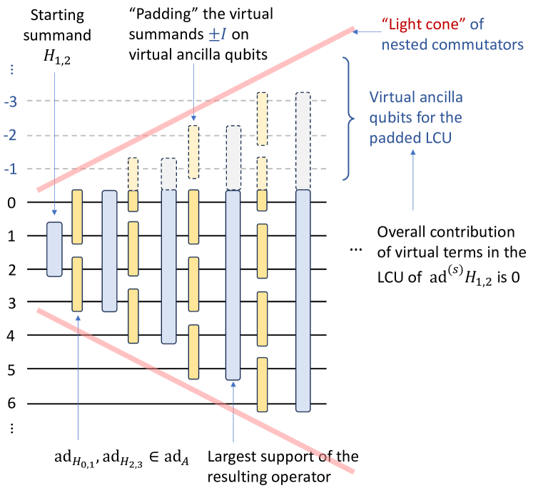
A problem of sampling the Hamiltonian summands Hj,j+1H_{j,j+1} in the commutator is that, since the Hamiltonian HH may be nonhomogeneous, the 11-norm of Hj,j+1H_{j,j+1} with different jj may be different. This will complicate the sampling algorithm, since we need to first calculate the 11-norm of all the elementary commutators with the form of

adHj2,j2+1adHj1,j1+1Hj,j+1,\mathrm{ad}_{H_{j_{2},j_{2}+1}}\mathrm{ad}_{H_{j_{1},j_{1}+1}}H_{j,j+1}, (16)

for all j,j1j,j_{1} and j2j_{2}. When the Trotter order KK and the expansion order s=K+1,,2K+1s=K+1,...,2K+1 gets larger, the number of elementary adjoint operators will increase exponentially. Consequently, we cannot estimate the 11-norm of all the elementary commutator.

To solve this problem but still keep the advantage of the NCC algorithm, we introduce the following Hamiltonian “padding” technique to ensure all the elementary nested commutator own the same 11-norm. Consider a Hamiltonian summand Hj,j+1H_{j,j+1}, which can be expanded to some Pauli operators,

Hj,j+1=ωαj(ω)Pj,j+1(ω),H_{j,j+1}=\sum_{\omega}\alpha_{j}^{(\omega)}P_{j,j+1}^{(\omega)}, (17)

where αj(ω)\alpha_{j}^{(\omega)} is a positive number and Pj,j+1(ω)P_{j,j+1}^{(\omega)} is a normalized Pauli operator whose support is on qubit jj and j+1j+1. Recall that Λ1:=maxjHj,j+11\Lambda_{1}:=\max_{j}\|H_{j,j+1}\|_{1} and Hj,j+11:=ωαj(ω)\|H_{j,j+1}\|_{1}:=\sum_{\omega}\alpha_{j}^{(\omega)}. When Hj,j+11\|H_{j,j+1}\|_{1} is smaller than Λ1\Lambda_{1}, we add extra trivial terms ±I\pm I in the Pauli decomposition of Hj,j+1H_{j,j+1},

H¯j,j+1\displaystyle\bar{H}_{j,j+1} =ωαj(ω)Pj,j+1(ω)+δΛ12I+δΛ12(I)\displaystyle=\sum_{\omega}\alpha_{j}^{(\omega)}P_{j,j+1}^{(\omega)}+\frac{\delta\Lambda_{1}}{2}I+\frac{\delta\Lambda_{1}}{2}(-I) (18)
=Λ1ωp¯j(ω)Pj,j+1(ω),\displaystyle=\Lambda_{1}\sum_{\omega}\bar{p}_{j}^{(\omega)}P_{j,j+1}^{(\omega)},

where δΛ1:=Λ1Hj,j+11\delta\Lambda_{1}:=\Lambda_{1}-\|H_{j,j+1}\|_{1}. Eq. 18 holds naturally, but now with a manually predetermined 11-norm value Λ1\Lambda_{1}. Similarly, we can pad all the elementary commutators with the form

adHj1,j1+1Hj,j+1=Hj1,j1+1Hj,j+1Hj,j+1Hj1,j1+1,\mathrm{ad}_{H_{j_{1},j_{1}+1}}H_{j,j+1}=H_{j_{1},j_{1}+1}H_{j,j+1}-H_{j,j+1}H_{j_{1},j_{1}+1}, (19)

so that their 11-norms are all 2Λ122\Lambda_{1}^{2}. In this way, we ignore the commutator relationship between Hj,j+1H_{j,j+1} and Hj1,j1+1H_{j_{1},j_{1}+1} as long as they are in the light-cone region.

After the padding procedure described above, all elementary nested commutators of the same order will have the same 11-norm. This property allows us to uniformly sample these commutators: the starting summand Hj,j+1H_{j,j+1} is sampled uniformly from those in BB, and the subsequent Hj1,j1+1H_{j_{1},j_{1}+1} and Hj2,j2+1H_{j_{2},j_{2}+1} are sampled uniformly within the light-cone region. However, when the starting summand Hj,j+1H_{j,j+1} is near the boundary, applying a few adjoint operators may cause it to touch the boundary. This reduces the number of possible elementary nested commutators compared to those starting from the center, resulting in different 11-norms for adAHj,j+1\text{ad}_{A}H_{j,j+1} depending on jj. This complicates the sampling of the starting summand Hj,j+1H_{j,j+1}. To resolve this issue and ensure uniform sampling of Hj,j+1H_{j,j+1}, we introduce virtual qubits at the boundary, as illustrated in Fig. 6, and pad the virtual qubits with 0-summed ±I\pm I terms. Since we only perform ±I\pm I operation on the virtual qubits, we do not need to introduce it in the real experiments.

We remark that, our padding method preserve the locality structure. As a result, the performance guarantee in Theorem 2 still holds. We summarize the sampling algorithm in Fig. 7. If we consider the Heisenberg Hamiltonian

H=iσiσi+1+iZi,H=\sum_{i}\vec{\sigma}_{i}\vec{\sigma}_{i+1}+\sum_{i}Z_{i}, (20)

as an example, where σi:=(Xi,Yi,Zi)\vec{\sigma}_{i}:=(X_{i},Y_{i},Z_{i}) is the vector of Pauli operators on the iith qubit, we can define the summand Hj,j+1H_{j,j+1} to be

Hj,j+1=4(14XjXj+1+14YjYj+1+14ZjZj+1+14Zj).H_{j,j+1}=4\left(\frac{1}{4}X_{j}X_{j+1}+\frac{1}{4}Y_{j}Y_{j+1}+\frac{1}{4}Z_{j}Z_{j+1}+\frac{1}{4}Z_{j}\right). (21)

In this case, Λ1=Hj,j+1=4\Lambda_{1}=\|H_{j,j+1}\|=4. The probability distribution p¯j(ω)\bar{p}_{j}^{(\omega)} in Fig. 7 is to uniformly sample the XXXX, YYYY, ZZZZ and ZIZI term. As a demonstration, we explicitly present the algorithm to sample the Pauli-rotation operator in the first-order NCC algortihm for the Heisenberg Hamiltonian in Eq. 20 in Algorithm 1.

Algorithm 1 Demonstration: sampling of ViV_{i} or VjV_{j} of first-order NCC algorithm for the Heisenberg Hamiltonian in Eq. 20
1:An nn-qubit Heisenberg Hamiltonian HH in Eq. 20; unit evolution time 0<x<10<x<1 for each Trotter segment;
2:Sampling of a Pauli-rotation operator ViV_{i} from the Trotter remainder V~1(nc)(x)\tilde{V}_{1}^{(nc)}(x).
3:Sample the expansion order s{2,3}s\in\{2,3\} with the probability {11+24x,24x1+24x}\{\frac{1}{1+24x},\frac{24x}{1+24x}\}.
4:if s=3s=3 then
5:  Sample the adjoint form ad(2)B\mathrm{ad}^{(2)}B from {adBadAB,adA2B}\{\mathrm{ad}_{B}\mathrm{ad}_{A}B,\mathrm{ad}_{A}^{2}B\} with the probability {1/3,2/3}\{1/3,2/3\}.
6:end if
7:Sample the starting index jj uniformly from all odd indices in 0,,n10,...,n-1. Sample the Pauli operator Pj,j+1P_{j,j+1} uniformly from {XX,YY,ZZ,ZI}\{XX,YY,ZZ,ZI\} on qubit jj and j+1j+1.
8:Set W:=Pj,j+1W:=P_{j,j+1}.
9:Sample the adjoint index j1j_{1} uniformly from {j1,j+1}\{j-1,j+1\}. Sample the Pauli operator Pj1,j1+1P_{j_{1},j_{1}+1} uniformly from {XX,YY,ZZ,ZI}\{XX,YY,ZZ,ZI\} on qubit j1j_{1} and j1+1j_{1}+1. Sample the multiplication order b1b_{1} uniformly from {0,1}\{0,1\}. 111If j1j-1 or j+1j+1 exceeds the index range 0,,n10,...,n-1, we pad extra virtual qubits similar to Fig. 6.
10:if b1=0b_{1}=0 then
11:  Set W:=Pj1,j1+1WW:=P_{j_{1},j_{1}+1}W.
12:else\triangleright b1=1b_{1}=1
13:  Set W:=WPj1,j1+1W:=-WP_{j_{1},j_{1}+1}.
14:end if
15:if s=3s=3 then
16:  if ad(2)B=adBadAB\mathrm{ad}^{(2)}B=\mathrm{ad}_{B}\mathrm{ad}_{A}B then
17:   Sample the adjoint index j2j_{2} uniformly from {j2,j,j+2}\{j-2,j,j+2\}. Sample the Pauli operator Pj2,j2+1P_{j_{2},j_{2}+1} uniformly from {XX,YY,ZZ,ZI}\{XX,YY,ZZ,ZI\} on qubit j2j_{2} and j2+1j_{2}+1. Sample the multiplication order b2b_{2} uniformly from {0,1}\{0,1\}.
18:  else\triangleright ad(2)B=adA2B\mathrm{ad}^{(2)}B=\mathrm{ad}_{A}^{2}B
19:   Sample the adjoint index j2j_{2} uniformly from {j3,j1,j+1}\{j-3,j-1,j+1\}. Sample the Pauli operator Pj2,j2+1P_{j_{2},j_{2}+1} uniformly from {XX,YY,ZZ,ZI}\{XX,YY,ZZ,ZI\} on qubit j2j_{2} and j2+1j_{2}+1. Sample the multiplication order b2b_{2} uniformly from {0,1}\{0,1\}.
20:  end if
21:  if b2=0b_{2}=0 then
22:   Set W:=Pj2,j2+1WW:=P_{j_{2},j_{2}+1}W.
23:  else\triangleright b2=1b_{2}=1
24:   Set W:=WPj2,j2+1W:=-WP_{j_{2},j_{2}+1}.
25:  end if
26:end if
27:Return Vi:=exp(iθW)V_{i}:=\exp\left(i\theta W\right) as the sampled Pauli-rotation operator. Here θ:=tan1(16nx2(1+24x))\theta:=\tan^{-1}(16nx^{2}(1+24x)).
Refer to caption
Figure 7: The sampling procedure of ViV_{i} or VjV_{j} in Fig. 2(b) in the NCC algorithm. We set K=1K=1 as example. The notation l:l+kl:l+k indicates the number array of l,l+1,,l+kl,l+1,...,l+k. blb_{l} determines whether to multiply Pjl,jl+1(ωl)P_{j_{l},j_{l}+1}^{(\omega_{l})} to the left or the right side of the current Pauli operator. U()\mathrm{U}(\bullet) refers to a uniform distribution in the set. ηΣ(nc):=F1.2(nc)1+F1.3(nc)1\eta_{\Sigma}^{(nc)}:=\|F_{1.2}^{(nc)}\|_{1}+\|F_{1.3}^{(nc)}\|_{1}. θ(y):=tan1(y)\theta(y):=\tan^{-1}(y). The probability p¯j(ω)\bar{p}_{j}^{(\omega)} is given by the Hamiltonian information in Eq. 18.

As a final remark, the sampling procedure in both PTSC and NCC algorithms are independent of the implementation of the quantum circuit and the measurement outcome. Thanks to this property, we can perform the classical sampling during the quantum circuit implementation or even generate the sampled Pauli matrices before the implementation of the quantum circuits.

II.5 Performance comparison

In Table 1, we compare the implementation complexity and the gate complexity in a single round of experiment of the 0th-order PTSC, KKth-order PTSC, and KKth-order NCC algorithms to previous Hamiltonian simulation algorithms. For a fair comparison, we set the 1-norm of all LCU formulas μ\mu to be constant. In this case, the sample complexity of PTSC and NCC algorithms incurs a μ4\mu^{4} overhead compared to standard sampling from the KKth-order Trotter or post-Trotter algorithms.

We show that by inserting a few randomly sampled Pauli-rotation gates after each Trotter segment, as illustrated in Fig. 1, both PTSC and NCC achieve improved accuracy and time dependence. The gate counts for PTSC exhibit logarithmic dependence on accuracy, log(1/ε)\log(1/\varepsilon), while the NCC gate counts show improved system-size dependence.

Algorithm Implementation hardness Accuracy Size scaling (lattice Hamiltonian) Time dependence
KKth-order Trotter Suzuki (1990) Easy 𝒪(ε1/K)\mathcal{O}(\varepsilon^{-1/K}) 𝒪(n1+1K)\mathcal{O}(n^{1+\frac{1}{K}}) 𝒪(t1+1K)\mathcal{O}(t^{1+\frac{1}{K}})
Post-Trotter Berry et al. (2015); Low and Chuang (2019) Hard 𝒪(log~(1/ε))\mathcal{O}(\tilde{\log}(1/\varepsilon)) 𝒪(n2)\mathcal{O}(n^{2}) 𝒪(t)\mathcal{O}(t)
0th-order PTSC Easy 𝒪(log~(1/ε))\mathcal{O}(\tilde{\log}(1/\varepsilon)) 𝒪(n2)\mathcal{O}(n^{2}) 𝒪(t2)\mathcal{O}(t^{2})
KKth-order PTSC Easy 𝒪(log~(1/ε))\mathcal{O}(\tilde{\log}(1/\varepsilon)) 𝒪(n2+12K+1)\mathcal{O}(n^{2+\frac{1}{2K+1}}) 𝒪(t1+12K+1)\mathcal{O}(t^{1+\frac{1}{2K+1}})
KKth-order NCC Easy 𝒪(ε1/(2K+1))\mathcal{O}(\varepsilon^{-1/(2K+1)}) 𝒪(n1+22K+1)\mathcal{O}(n^{1+\frac{2}{2K+1}}) 𝒪(t1+12K+1)\mathcal{O}(t^{1+\frac{1}{2K+1}})
Table 1: Comparison of the implementation hardness and gate complexity in a single round of the circuit for Trotter-LCU methods versus previous algorithms. Here, log~(x):=log(x)/loglog(x)\tilde{\log}(x):=\log(x)/\log\log(x). The (implementation) hardness refers to whether one needs to implement multicontrolled gates with plenty of ancillary qubits. In the comparison for the system-size scaling of lattice Hamiltonians, we use the fact that λ=𝒪(n)\lambda=\mathcal{O}(n) and L=𝒪(n)L=\mathcal{O}(n).

To demonstrate how the Trotter-LCU algorithms can help reduce gate costs in practical scenarios, we estimate the single-shot gate count of random-sampling Trotter-LCU algorithms and compare it with the state-of-the-art Trotter algorithm, i.e., fourth-order Trotter Suzuki (1991); Childs et al. (2019, 2021). To ensure a fair comparison, we set 11-norm of the LCU formula to be μ=2\mu=2. Based on Proposition 1, this implies that the random-sampling Trotter-LCU algorithm will require an additional factor of 1616 in the sample number to estimate the properties of the target state UρUU\rho U^{\dagger} where U:=eiHtU:=e^{iHt} to a given precision compared to the normal Trotter or coherent implementation of LCU algorithms.

We compile their quantum circuits to 𝒞𝒩𝒪𝒯\mathcal{CNOT} gates, single-qubit Clifford gates, and single-qubit ZZ-axis rotation gates Rz(θ)=eiθZR_{z}(\theta)=e^{i\theta Z}. Here, we mainly compare the number of Rz(θ)R_{z}(\theta) gates since they are the most resource-consuming part on a fault-tolerant quantum computer Litinski (2019). The 𝒞𝒩𝒪𝒯\mathcal{CNOT} gate-number comparison results can be found in Appendix G, which is similar to the Rz(θ)R_{z}(\theta) gate comparison. We also compare the gate counts of the Trotter-LCU algorithms to the coherent-implementation of LCU Berry et al. (2014, 2015) and QSP Low and Chuang (2017, 2019) in Appendix G.

In the first comparison, we consider the simulation of generic Hamiltonians without the usage of commutator information, for which we choose the 22-local Hamiltonian, H=i,jXiXj+iZiH=\sum_{i,j}X_{i}X_{j}+\sum_{i}Z_{i} where XiX_{i} and ZiZ_{i} are the Pauli matrices on the iith qubit. Fig. 8(a,b) show the gate counts for the fourth-order Trotter formula and the PTSC Trotter-LCU algorithms with different orders with an increasing time tt and increasing system size nn, respectively. The gate counting method for fourth-order Trotter with random permutation is based on the analytical bounds in Ref. Childs et al. (2019).

Refer to caption
Figure 8: Non-Clifford Rz(θ)R_{z}(\theta) gate-number estimation for simulating real-time dynamics with Trotter and Trotter-LCU algorithms. (a) and (b) show the Rz(θ)R_{z}(\theta) gate counts when simulating the Hamiltonian H=i,jXiXj+iZiH=\sum_{i,j}X_{i}X_{j}+\sum_{i}Z_{i}. (a) shows the Rz(θ)R_{z}(\theta) gate count with an increasing time and fixed system-size n=20n=20. (b) shows the Rz(θ)R_{z}(\theta) gate count with an increasing system size with the time t=nt=n. We list the performance of zeroth, second, and fourth-order PTSC algorithms with μ=2\mu=2. The fourth-order Trotter analytical bound is from Ref. Childs et al. (2019). (c) The Rz(θ)R_{z}(\theta) gate count for the nearest-interaction Heisenberg model using the nested-commutator bound with n=12n=12 and n=50n=50. The fourth-order Trotter commutator bound is from Ref. Childs et al. (2021).

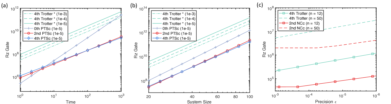
From Fig. 8(a,b), we can clearly see the advantage of composition of Trotter and LCU formulas: if we do not use LCU and merely apply Trotter formulas, the gate resource of fourth-order Trotter suffers from a large overhead that is 2 orders of magnitudes larger than the PTSC algorithms. Moreover, if we increase ε\varepsilon from 10310^{-3} to 10510^{-5}, we can see a clear increase of the gate resources for the Trotter algorithm. For the PTSC algorithms, however, the gate number is almost not affected by ε\varepsilon since they enjoy a logarithmic ε\varepsilon-dependence.

On the other hand, if we do not use Trotter formula, the 0th-order PTSC algorithm owns a quadratically worse tt-dependence (𝒪(t2)\mathcal{O}(t^{2})) than the fourth-order Trotter (𝒪(t1.25)\mathcal{O}(t^{1.25})), second-order PTSC (𝒪(t1.2)\mathcal{O}(t^{1.2})) and fourth-order PTSC (𝒪(t1.11)\mathcal{O}(t^{1.11})) algorithms in Fig. 8(a). For a short-time evolution t=nt=n, the system-size dependence of second- or fourth-order PTSC in Fig. 8(b) outperforms 0th-order PTSC algorithm. In the case when long-time Hamiltonian simulation is required, for example, tt should be set to 10310^{3} for the phase estimation Campbell (2019), the advantage of 22nd or fourth-order PTSC to 0th-order PTSC will be more obvious. The composition of Trotter and LCU formulas enables 22nd or fourth-order PTSC to enjoy good tt and ε\varepsilon dependence and small gate-resource overhead simultaneously.

Next, we compare the gate count when simulating the lattice models, where the commutator analysis will help remarkably reduce the gate count. We consider the Heisenberg Hamiltonian H=iσiσi+1+iZiH=\sum_{i}\vec{\sigma}_{i}\vec{\sigma}_{i+1}+\sum_{i}Z_{i} using the nested-commutator bounds. In Fig. 8(c), we choose n=t=12n=t=12 and 5050 and show the gate number with respect to the accuracy requirement ε\varepsilon. The fourth-order Trotter error analysis is based on the nested-commutator bound (Proposition M.1 in Ref. Childs et al. (2021)), which is currently the tightest Trotter error analysis. The performance of our second-order NCC algorithm is based on the analytical bound in Sec. H in the Appendix. We mainly present results for the second-order NCC algorithm due to its simplicity and leave precise higher-order NCC gate count analysis for future study.

From Fig. 8(c), we can see that, while enjoying near-optimal system-size scaling similar to the fourth-order Trotter algorithm which is currently the best one for lattice Hamiltonians Childs et al. (2021); Childs and Su (2019), the second-order NCC algorithm shows better accuracy dependence than fourth-order Trotter algorithm. Particularly, using the same gate number as the fourth-order Trotter, we are able to achieve a 3 to 4 orders of magnitudes higher accuracy ε\varepsilon.

III PRELIMINARIES

In this section, we review the Hamiltonian simulation algorithms based on Trotter and LCU formulas.

In all the Hamiltonian simulation algorithms discussed in this work, we divide the real-time evolution U(t)U(t) into ν\nu segments,

U(t)=eiHt=(U(x))ν=(eiHx)ν,U(t)=e^{-iHt}=(U(x))^{\nu}=\left(e^{-iHx}\right)^{\nu}, (22)

with x:=t/νx:=t/\nu, and consider the construction of each small segment U(x)U(x). Without loss of generality, we assume x>0x>0.

III.1 Trotter formulas

The most natural way to approximate U(x)U(x) is to apply the Lie-Trotter-Suzuki formulas Suzuki (1990, 1991). Hereafter, we refer to them as Trotter formulas. The first-order Trotter formula is

S1(x)=l=1LeixHl=eixHLeixH2eixH1=:eixH.\displaystyle S_{1}(x)=\prod_{l=1}^{L}e^{-ixH_{l}}=e^{-ixH_{L}}.e^{-ixH_{2}}e^{-ixH_{1}}=:\prod^{\leftarrow}e^{-ix\vec{H}}. (23)

Here, H:=[H1,H2,,HL]\vec{H}:=[H_{1},H_{2},...,H_{L}]. In Eq. 23, we simplify the notation of the sequential products from l=1l=1 to LL with the same form, using the arrow to denote the ascending direction of the dummy index ll. The Hermitian conjugation of S1(x)S_{1}(x) can similarly be written as S1(x)=eixHS_{1}(x)^{\dagger}=\overset{\rightarrow}{\prod}e^{ix\vec{H}}.

The second-order Trotter formula is

S2(x)\displaystyle S_{2}(x) =D2(x)D2(x)=S1(x2)S1(x2)\displaystyle=D_{2}(-x)^{\dagger}D_{2}(x)=S_{1}(-\frac{x}{2})^{\dagger}S_{1}(\frac{x}{2}) (24)
=ei12xHei12xH,\displaystyle=\prod^{\rightarrow}e^{-i\frac{1}{2}x\vec{H}}\prod^{\leftarrow}e^{-i\frac{1}{2}x\vec{H}},

where D2(x):=S1(x2)D_{2}(x):=S_{1}(\frac{x}{2}). We have S2(x)=S2(x)S_{2}(-x)^{\dagger}=S_{2}(x).

The general 2k2kth-order Trotter formula is Suzuki (1991)

S2k(x)\displaystyle S_{2k}(x) =D2k(x)D2k(x)\displaystyle=D_{2k}(-x)^{\dagger}D_{2k}(x) (25)
=[S2k2(ukx)]2S2k2((14uk)x)[S2k2(ukx)]2,\displaystyle=[S_{2k-2}(u_{k}x)]^{2}S_{2k-2}((1-4u_{k})x)[S_{2k-2}(u_{k}x)]^{2},

with uk:=1/(441/(2k1))u_{k}:=1/(4-4^{1/(2k-1)}) for k1k\geq 1. The operator D2k(x)D_{2k}(x) is defined recursively,

D2k(x):=D2k2((14uk)x)S2k2(ukx)2.D_{2k}(x):=D_{2k-2}((1-4u_{k})x)S_{2k-2}(u_{k}x)^{2}. (26)

By induction from Eq. 25 and Eq. 26 we can show that S2k(x)=S2k(x)S_{2k}(-x)^{\dagger}=S_{2k}(x).

We also denote the zeroth-order Trotter formula to be S0(x)=IS_{0}(x)=I for consistency. We denote the multiplicative remainder of the Trotter formulas as

VK(x)\displaystyle V_{K}(x) =U(x)SK(x),\displaystyle=U(x)S_{K}(x)^{\dagger}, (27)

for K=0,1,2kK=0,1,2k. In what follows, we name this Trotter error term VK(x)V_{K}(x) as the KKth-order Trotter remainder to avoid ambiguity to other error effects such as truncation error.

In Ref. Suzuki (1990), Suzuki proves the following order condition for the Trotter formulas,

SK(x)=U(x)+𝒪(xK+1)=eiHx+𝒪(xK+1),S_{K}(x)=U(x)+\mathcal{O}(x^{K+1})=e^{-iHx+\mathcal{O}(x^{K+1})}, (28)

for K=1K=1 or even positive KK. As a result, the remainder VK(x)V_{K}(x) will only contain the terms of xqx^{q} with qK+1q\geq K+1. We will use the following order condition of Trotter formulas in the later discussion.

Lemma 1 (Order condition of Trotter formulas, Theorem 4 in Childs et al. (2021)).

Let HH be an Hermitian operator and U(x):=eiHxU(x):=e^{-iHx} to be the time-evolution operator with xx\in\mathbb{R}. For the Trotter formula SK(x)S_{K}(x) defined in Eq. 23 and Eq. 25, where K=1K=1 or positive even number, we have the following

  1. 1.

    Additive error: AK(x):=SK(x)U(x)=𝒪(xK+1)A_{K}(x):=S_{K}(x)-U(x)=\mathcal{O}(x^{K+1}),

  2. 2.

    Multiplicative error: MK(x):=U(x)SK(x)I=𝒪(xK+1)M_{K}(x):=U(x)S_{K}(x)^{\dagger}-I=\mathcal{O}(x^{K+1}),

  3. 3.

    For the exponentiated error EK(x)E_{K}(x) such that SK(x)=𝒯exp(0x𝑑τ(iH+EK(τ)))S_{K}(x)=\mathcal{T}\exp\left(\int_{0}^{x}d\tau(-iH+E_{K}(\tau))\right), we have EK(x)=𝒪(xK)E_{K}(x)=\mathcal{O}(x^{K}).

III.2 LCU formulas

Instead of decomposing U(x)U(x) as a product of elementary unitaries, another way is to decompose U(x)U(x) to a summation of elementary unitaries. We now provide a formal definition of a LCU formula.

Definition 1 (Childs and Wiebe (2012)).

A (μ,ε)(\mu,\varepsilon) (LCU) formula of an operator VV is defined to be

V~=i=0Γ1ciVi=μi=0Γ1Pr(i)Vi,\tilde{V}=\sum_{i=0}^{\Gamma-1}c_{i}V_{i}=\mu\sum_{i=0}^{\Gamma-1}\Pr(i)V_{i}, (29)

such that the spectral norm distance VV~ε\|V-\tilde{V}\|\leq\varepsilon. Here, μ>0\mu>0 is the l1l_{1}-norm of the coefficient vector, Pr(i)\Pr(i) is a probability distribution over different unitaries ViV_{i}, and {Vi}i=0Γ1\{V_{i}\}_{i=0}^{\Gamma-1} is a set of unitaries. Here, we assume ci>0c_{i}>0 for all ii and absorb the phase into the unitaries ViV_{i}. We call μ\mu the 11-norm of this (μ,ε)(\mu,\varepsilon)-LCU formula.

In what follows, we define the 11-norm V1\|V\|_{1} of an operator VV to be its smallest 11-norm over all possible (μ,0)(\mu,0)-LCU formulas for VV. Note that, U1=1\|U\|_{1}=1 for any unitary UU. One can easily check the validity of this norm definition.

We may consider two ways to implement the LCU formula of the operator VV. In the first way, we coherently implement the LCU formula by introducing an ancillary system AA with the dimension Γ\Gamma which costs log2Γ\lceil\log_{2}\Gamma\rceil qubits. For the LCU lemma defined in Eq. 29, we define the amplitude-encoding unitary UAEU_{AE} and the select gate Sel(V~)\mathrm{Sel}(\tilde{V}) to be,

UAE|0A\displaystyle U_{AE}\ket{0}_{A} :=i=0Γ1Pr(i)|i,\displaystyle=\sum_{i=0}^{\Gamma-1}\sqrt{\Pr(i)}\ket{i}, (30)
Sel(V~)\displaystyle\mathrm{Sel}(\tilde{V}) :=i=0Γ1|ii|Vi.\displaystyle=\sum_{i=0}^{\Gamma-1}\ket{i}\bra{i}\otimes V_{i}.

Then, the following controlled-gate WABW_{AB} acting on ancillary AA and system BB defines a way to realize LCU coherently when we prepare |0\ket{0} on AA and measure it on computational basis to get |0\ket{0},

W:=(UAEI)Sel(V~)(UAEI).W:=(U_{AE}^{\dagger}\otimes I)\mathrm{Sel}(\tilde{V})(U_{AE}\otimes I). (31)

More precisely, if we set the initial state on BB to be |ψ\ket{\psi}, then we have

W|0A|ψB=1μ|0A(V~|ψ)B+11μ2|ΦAB,W\ket{0}_{A}\ket{\psi}_{B}=\frac{1}{\mu}\ket{0}_{A}\left(\tilde{V}\ket{\psi}\right)_{B}+\sqrt{1-\frac{1}{\mu^{2}}}\ket{\Phi_{\perp}}_{AB}, (32)

where |ΦAB\ket{\Phi_{\perp}}_{AB} is a state whose ancillary state is supported in the subspace orthogonal to |0\ket{0}.

If we perform computation-basis measurement directly on AA, the successful probability to obtain V~|ψ\tilde{V}\ket{\psi} is 1μ2\frac{1}{\mu^{2}}. To boost the successful probability to nearly deterministic, we can introduce the amplitude amplification techniques Berry et al. (2014). To this end, we consider the following isometry

𝒱:=WRWRW(|0I)AB.\mathcal{V}:=-WRW^{\dagger}RW\left(\ket{0}\otimes I\right)_{AB}. (33)

Here, RR is a reflection over |0\ket{0} on the system AA,

R=I2|0A0|.R=I-2\ket{0}_{A}\bra{0}. (34)

Consider the case of μ=2\mu=2 and ε\varepsilon is small for the LCU formula. If V~\tilde{V} is a unitary, then we have (0|I)𝒱=V~(\bra{0}\otimes I)\mathcal{V}=\tilde{V}. For a general V~\tilde{V}, we can verify the resulting operator

(0|I)𝒱=32V~12V~V~V~,(\bra{0}\otimes I)\mathcal{V}=\frac{3}{2}\tilde{V}-\frac{1}{2}\tilde{V}\tilde{V}^{\dagger}\tilde{V}, (35)

is close to VV with the spectral norm distance bound ξ:=(ε2+3ε+4)ε/2\xi:=(\varepsilon^{2}+3\varepsilon+4)\varepsilon/2. Also, the successful probability to project the ancilla to |0\ket{0} is larger than (1ξ)2(1-\xi)^{2}.

In the second way to implement the LCU formula, we randomly sample the terms {Vi}\{V_{i}\} in Eq. 29 based on the probability Pr(i)\Pr(i) Childs and Wiebe (2012). This way saves the ancillary qubit number and the cost to implement the multiqubit Toffoli gates in UAEU_{AE} and Sel(V~)\mathrm{Sel}(\tilde{V}) in Eq. 30, which is more suitable to implement in the near-term devices. Instead of implementing the operator VV directly, we now focus on the task to estimate the properties of the target state σ=VρV\sigma=V\rho V^{\dagger} where ρ\rho is the initial state of the Hamiltonian simulation task. Suppose we want to estimate expectation value of a given observable OO on σ\sigma, we can then embed the task to Hadamard test Kitaev (1995) shown in Fig. 9.

Refer to caption
Figure 9: Estimate the observable value Tr(VρVO)\mathrm{Tr}(V\rho V^{\dagger}O) based on the random sampling implementation of (μ,ε)(\mu,\varepsilon)-LCU formula of VV defined in Eq. 29.

We first prepare a |+\ket{+} state on a single ancillary qubit. After that, we implement two controlled operations |0A0|IB+|1B1|(Vi)B\ket{0}_{A}\bra{0}\otimes I_{B}+\ket{1}_{B}\bra{1}\otimes(V_{i})_{B} and |0A0|(Vj)B+|1B1|IB\ket{0}_{A}\bra{0}\otimes(V_{j})_{B}+\ket{1}_{B}\bra{1}\otimes I_{B} where ViV_{i} and VjV_{j} are sampled independently from the LCU formula in Eq. 29. The measured expectation value of μ2XAOB\langle\mu^{2}X_{A}\otimes O_{B}\rangle is then a nearly unbiased estimation of Tr(VρVO)\mathrm{Tr}(V\rho V^{\dagger}O). We will use the following performance guarantee for the observable estimation.

Proposition 1 (Performance of the random-sampling LCU implementation, Theorem 2 from Faehrmann et al. (2022)).

For a target operator VV and its (μ,ε)(\mu,\varepsilon)-LCU formula defined in Definition 1, if we estimate the value OV:=Tr(VρVO)\braket{O}_{V}:=\mathrm{Tr}(V\rho V^{\dagger}O) with an initial state ρ\rho and observable OO using the circuit in Fig. 9 for NN times, then the distance between the mean estimator value O^\hat{O} and the true value OV\braket{O}_{V} is bounded by

|O^OV|O(3ε+εn),|\hat{O}-\braket{O}_{V}|\leq\|O\|(3\varepsilon+\varepsilon_{n}), (36)

with successful probability 1δ1-\delta. Here, N=2μ4ln(2/δ)/εn2N=2\mu^{4}\ln(2/\delta)/\varepsilon_{n}^{2}, O\|O\| is the spectral norm of OO.

From Proposition 1 we can see that, the 11-norm μ\mu of the LCU formula affects the sample complexity while the accuracy factor ε\varepsilon introduces extra bias in the observable estimation. To estimate OV\langle O\rangle_{V} using Hadamard-test-type circuits with ε\varepsilon accuracy, we need 𝒪(μ4/ε2)\mathcal{O}(\mu^{4}/\varepsilon^{2}) sampling resource, which owns an extra μ4\mu^{4} overhead compared to the normal Hamiltonian simulation algorithms Faehrmann et al. (2022). To make the algorithm efficient, we need to set μ\mu to be a constant.

In the later discussion, we will construct new LCU formulas from the product of LCU formulas. We will use following proposition.

Proposition 2 (Product of LCU formulas).

Suppose we have a (μ,ε)(\mu,\varepsilon)-LCU formula V~\tilde{V} for an operator VV with the form of Eq. 29. Then the product formula

V~ν=μνi1,i2,,iνPr(i1)Pr(i2)Pr(iν)V1V2Vν,ν,\tilde{V}^{\nu}=\mu^{\nu}\sum_{i_{1},i_{2},...,i_{\nu}}\Pr(i_{1})\Pr(i_{2})...\Pr(i_{\nu})V_{1}V_{2}...V_{\nu},\quad\nu\in\mathbb{N}, (37)

is a (μ,ε)(\mu^{\prime},\varepsilon^{\prime})-LCU formula for VνV^{\nu} with

μ=μν,ενμε.\mu^{\prime}=\mu^{\nu},\quad\varepsilon^{\prime}\leq\nu\mu^{\prime}\varepsilon. (38)
Proof.

The 11-norm is obvious. We now bound the distance ε\varepsilon^{\prime} between U~ν\tilde{U}^{\nu} and UνU^{\nu}.

UνU~ν\displaystyle\|U^{\nu}-\tilde{U}^{\nu}\| =k=1νUk1(UU~)U~νk\displaystyle=\left\|\sum_{k=1}^{\nu}U^{k-1}(U-\tilde{U})\tilde{U}^{\nu-k}\right\|
k=1νUk1UU~U~νk\displaystyle\leq\sum_{k=1}^{\nu}\|U^{k-1}\|\|U-\tilde{U}\|\|\tilde{U}^{\nu-k}\|
νUU~k=1νmax{U,U~}ν1\displaystyle\leq\nu\|U-\tilde{U}\|\sum_{k=1}^{\nu}\max\{\|U\|,\|\tilde{U}\|\}^{\nu-1} (39)
νεμν1νμε.\displaystyle\leq\nu\varepsilon\mu^{\nu-1}\leq\nu\mu^{\prime}\varepsilon.

We remark that, when there are common unitary components for all {Vi}\{V_{i}\} in the LCU formula Eq. 29, we can simplify the circuit in Fig. 9 by removing the ancillary control on the common unitary components. Suppose we have the following LCU formula for an operator VV,

V~=μi1,i2,,iνPr(i1,i2,,iν)ViνWνVi2W2Vi1W1,\tilde{V}=\mu\sum_{i_{1},i_{2},...,i_{\nu}}\Pr(i_{1},i_{2},...,i_{\nu})V_{i_{\nu}}W_{\nu}...V_{i_{2}}W_{2}V_{i_{1}}W_{1}, (40)

such that VV~ε\|V-\tilde{V}\|\leq\varepsilon, where W1,W2,,WνW_{1},W_{2},...,W_{\nu} are some fixed unitaries. Then according to Definition 1, Eq. 40 is a (μ,ε)(\mu,\varepsilon)-LCU formula of VV with the elementary unitaries to be Vi=ViνWνVi2W2Vi1W1V_{\vec{i}}=V_{i_{\nu}}W_{\nu}...V_{i_{2}}W_{2}V_{i_{1}}W_{1} for i={i1,i2,,iν}\vec{i}=\{i_{1},i_{2},...,i_{\nu}\}. Instead of naively apply the Hadamard test circuit in Fig. 9, we can introduce an equivalent circuit implementation shown in Fig. 10(b). The performance guarantee in Proposition 1 also holds for the improved implementation.

Refer to caption
Figure 10: Improve the random-sampling implementation of Hamiltonian simulation based on (μ,ε)(\mu,\varepsilon)-LCU formula in Eq. 40. (a) The LCU formula of VV in Eq. 40 with deterministic components. (b) The improved application of Hadamard test. We remove the control on the fixed unitaries and apply them only once. (c) A variant of Hadamard test, where the ancillary qubit is measured and reset for each randomly sampled unitary VikV_{i_{k}} for k=1,,νk=1,...,\nu.

Furthermore, we notice that Tr(OV~ρV~)\mathrm{Tr}(O\tilde{V}\rho\tilde{V}^{\dagger}) can be written as,

𝔼i1,j1;;iν,jνTr[Oiν,jν𝒲νi1,j1𝒲1(ρ)],\displaystyle\mathbb{E}_{i_{1},j_{1};...;i_{\nu},j_{\nu}}\mathrm{Tr}[O\,\mathcal{E}_{i_{\nu},j_{\nu}}\circ\mathcal{W}_{\nu}\circ\,.\,\circ\mathcal{E}_{i_{1},j_{1}}\circ\mathcal{W}_{1}(\rho)], (41)

where 𝒲k():=WkWk\mathcal{W}_{k}(\bullet):=W_{k}\bullet W_{k}^{\dagger} and ik,jk():=12(VikVjk+VjkVik)\mathcal{E}_{i_{k},j_{k}}(\bullet):=\frac{1}{2}(V_{i_{k}}\bullet V_{j_{k}}^{\dagger}+V_{j_{k}}\bullet V_{i_{k}}^{\dagger}) for k=1,2,,νk=1,2,...,\nu. As a result, we can implement each channel 𝒲k\mathcal{W}_{k} by a unitary and each map ik,jk\mathcal{E}_{i_{k},j_{k}} by a Hadamard-test-type circuit. This leads to a variant circuit shown in Fig. 10(c), where the ancillary qubit is measured and reset for every segment. While this circuit owns the same gate complexity as Fig. 10(b), it is beneficial in a fault-tolerant quantum computer since we do not need to store the ancillary qubit for a long time-the ancillary qubit is activated only in the compensation stage and is quickly measured.

IV Trotter-LCU algorithms with paired Taylor-series compensation

In this section, we construct a (μ,ε)(\mu,\varepsilon)-LCU formula for the remainder VK(x)V_{K}(x) of the KK-th order Trotter formula based on the idea to perform Taylor-series (TS) expansion on all the exponential terms in VK(x)V_{K}(x). Although TS expansion is naturally a LCU formula of VK(x)V_{K}(x), it usually owns poor μ\mu performance. To further suppress the 11-norm of the expansion, we will modify the introduce a “pairing” idea to combine the terms that correspond to different TS expansion orders. We first consider a simple case without Trotter formula in subsection IV.1 to illustrate the major idea to construct TS-based LCU formula. Then we take the construction of LCU for the first-order Trotter formula as an example in subsection IV.2. Finally, in subsection IV.3, we discuss the random-sampling implementation of the algorithm and analyze its sample and gate complexity.

IV.1 Zeroth-order case

We begin our discussion from the case where the Trotter formula is trivial, i.e., S0(x)=IS_{0}(x)=I for each segment. In this case, the Trotter remainder is V0(x)=U(x)=eixHV_{0}(x)=U(x)=e^{-ixH}. To construct LCU formula, we expand V0(x)V_{0}(x) by Taylor series Berry et al. (2015),

V0(x)\displaystyle V_{0}(x) =s=0(iλx)ss!l1,,lspl1pl2plsPl1Pl2Pls\displaystyle=\sum_{s=0}^{\infty}\frac{(-i\lambda x)^{s}}{s!}\sum_{l_{1},...,l_{s}}p_{l_{1}}p_{l_{2}}.p_{l_{s}}P_{l_{1}}P_{l_{2}}.P_{l_{s}} (42)
=s=0F0,s(x),\displaystyle=\sum_{s=0}^{\infty}F_{0,s}(x),

where

F0,s(x)=(iλx)ss!l1,,lspl1pl2plsPl1Pl2Pls.F_{0,s}(x)=\frac{(-i\lambda x)^{s}}{s!}\sum_{l_{1},...,l_{s}}p_{l_{1}}p_{l_{2}}...p_{l_{s}}P_{l_{1}}P_{l_{2}}...P_{l_{s}}. (43)

The 11-norm of V0(x)V_{0}(x) is

V0(x)1=s=0F0,s(x)1=1+(λx)+12!(λx)2+=eλx.\|V_{0}(x)\|_{1}=\sum_{s=0}^{\infty}\|F_{0,s}(x)\|_{1}=1+(\lambda x)+\frac{1}{2!}(\lambda x)^{2}+...=e^{\lambda x}. (44)

That is, the 11-norm of V0(x)V_{0}(x) is exponentially large with respect to λx\lambda x. Suppose we use V0(x)V_{0}(x) directly for the random-sampling implementation of LCU following Fig. 2(b), the composite LCU formula for U(t)=V0(x)νU(t)=V_{0}(x)^{\nu} is the product of V0(x)V_{0}(x). Based on Proposition 2, the 11-norm of the product formula is μ=(eλx)ν=eλt\mu=(e^{\lambda x})^{\nu}=e^{\lambda t}, which increases exponentially with the simulation time tt. Based on Proposition 1, this implies an exponentially increasing sample cost N=𝒪(μ4)N=\mathcal{O}(\mu^{4}). To make the TS expansion practical for the random-sampling implementation, we need to reduce 11-norm of V0(x)V_{0}(x).

When λx\lambda x is a small value, the major contribution to V0(x)1\|V_{0}(x)\|_{1} comes from the low-order terms of F0,s(x)F_{0,s}(x). Note that the first-order term F0,1(x)F_{0,1}(x) is anti-Hermitian. This allows us to utilize the following Euler’s formula on Pauli operators: for a Pauli matrix PP and yy\in\mathbb{R},

I+iyP=1+y2eiθ(y)P,I+iyP=\sqrt{1+y^{2}}e^{i\theta(y)P}, (45)

where θ(y):=tan1(y)\theta(y):=\tan^{-1}(y).

To suppress V0(x)1\|V_{0}(x)\|_{1}, we rewrite V0(x)V_{0}(x) as follows:

V0(x)=s=0F0,s(x)\displaystyle V_{0}(x)=\sum_{s=0}^{\infty}F_{0,s}(x) (46)
=Iiλxl=1LplPl+s=2F0,s(x)\displaystyle=I-i\lambda x\sum_{l=1}^{L}p_{l}P_{l}+\sum_{s=2}^{\infty}F_{0,s}(x)
=l=1Lpl(IiλxPl)+s=2F0,s(x).\displaystyle=\sum_{l=1}^{L}p_{l}(I-i\lambda xP_{l})+\sum_{s=2}^{\infty}F_{0,s}(x).

Then, we can apply Eq. 45 on Eq. 46 to convert the first-order term to Pauli rotation unitaries

V0(p)(x)=1+(λx)2l=1Lpleiθ0Pl+s=2F0,s(x),\displaystyle V_{0}^{(p)}(x)=\sqrt{1+(\lambda x)^{2}}\sum_{l=1}^{L}p_{l}e^{i\theta_{0}P_{l}}+\sum_{s=2}^{\infty}F_{0,s}(x), (47)

where θ0:=tan1(λx)\theta_{0}:=\tan^{-1}(-\lambda x). We call the formula in Eq. 47 the 0th-order PTS formula.

In practice, to avoid the sampling in the infinitely large space, we introduce a truncation sc2s_{c}\geq 2 to the expansion order of xx. After this truncation, the approximated LCU formula of V0(p)(x)V_{0}^{(p)}(x) is

V~0(p)(x):=U~0(p)(x)=1+(λx)2l=1Lpleiθ0Pl+s=2scF0,s(x)\displaystyle\tilde{V}_{0}^{(p)}(x)=\tilde{U}_{0}^{(p)}(x)=\sqrt{1+(\lambda x)^{2}}\sum_{l=1}^{L}p_{l}e^{i\theta_{0}P_{l}}+\sum_{s=2}^{s_{c}}F_{0,s}(x) (48)
=μ0(p)(x)(Pr0(p)(1)V0,1(p)+s=2scPr0(p)(s)V0,s(p)),\displaystyle=\mu_{0}^{(p)}(x)\left(\mathrm{Pr}_{0}^{(p)}(1)V_{0,1}^{(p)}+\sum_{s=2}^{s_{c}}\mathrm{Pr}_{0}^{(p)}(s)V_{0,s}^{(p)}\right),

where

μ0(p)(x)\displaystyle\mu_{0}^{(p)}(x) :=1+(λx)2+s=2scF0,s(x)1\displaystyle:=\sqrt{1+(\lambda x)^{2}}+\sum_{s=2}^{s_{c}}\|F_{0,s}(x)\|_{1}
1+(λx)2+(eλx1λx),\displaystyle\leq\sqrt{1+(\lambda x)^{2}}+\left(e^{\lambda x}-1-\lambda x\right),
Pr0(p)(s)\displaystyle\mathrm{Pr}_{0}^{(p)}(s) :=1μ0(p)(x){1+(λx)2,s=1,F0,s(x)1=(λx)ss!,s=2,3,,sc,\displaystyle:=\frac{1}{\mu_{0}^{(p)}(x)}\begin{cases}\sqrt{1+(\lambda x)^{2}},&s=1,\\ \|F_{0,s}(x)\|_{1}=\frac{(\lambda x)^{s}}{s!},&s=2,3,...,s_{c},\end{cases} (49)
V0,s(p)\displaystyle V_{0,s}^{(p)} :={lpleiθ0Pl,s=1,l1:spl1:s(s)(i)sPl1:s(s),s=2,3,,sc.\displaystyle:=\begin{cases}\sum_{l}p_{l}\,e^{i\theta_{0}P_{l}},&s=1,\\ \sum_{l_{1:s}}p_{l_{1:s}}^{(s)}(-i)^{s}P_{l_{1:s}}^{(s)},&s=2,3,...,s_{c}.\end{cases}

After “pairing” the terms with s=0s=0 and s=1s=1, we obtain Eq. 48 which is a new LCU formula with the 11-norm μ0(p)(x)\mu_{0}^{(p)}(x). We have the following proposition to characterize the LCU formula in Eq. 48.

Proposition 3 (0th-order Trotter-LCU formula by paired Taylor-series compensation).

For x0x\geq 0 and sc2s_{c}\geq 2, V~0(p)(x)\tilde{V}_{0}^{(p)}(x) in Eq. 48 is a (μ0(p)(x),ε0(p)(x))(\mu_{0}^{(p)}(x),\varepsilon_{0}^{(p)}(x))-LCU formula of V0(x)=U(x)V_{0}(x)=U(x) with

μ0(p)(x)e32(λx)2,ε0(p)(x)(eλxsc+1)sc+1.\mu_{0}^{(p)}(x)\leq e^{\frac{3}{2}(\lambda x)^{2}},\quad\varepsilon_{0}^{(p)}(x)\leq\left(\frac{e\lambda x}{s_{c}+1}\right)^{s_{c}+1}. (50)
Proof.

For the normalization factor, we have

μ0(p)(x)1+(λx)2+(eλx1λx)\displaystyle\mu_{0}^{(p)}(x)\leq\sqrt{1+(\lambda x)^{2}}+\left(e^{\lambda x}-1-\lambda x\right)
1+12(λx)2+(eλx1λx)\displaystyle\leq 1+\frac{1}{2}(\lambda x)^{2}+\left(e^{\lambda x}-1-\lambda x\right) (51)
e(λx)2+12(λx)2e32(λx)2.\displaystyle\leq e^{(\lambda x)^{2}}+\frac{1}{2}(\lambda x)^{2}\leq e^{\frac{3}{2}(\lambda x)^{2}}.

The fourth inequality is due to exxex2e^{x}-x\leq e^{x^{2}} for xx\in\mathbb{R}.

For the distance bound, we have

V~0(x)V0(x)s>scF0,s(x)\displaystyle\|\tilde{V}_{0}(x)-V_{0}(x)\|\leq\sum_{s>s_{c}}\|F_{0,s}(x)\| (52)
s>sc(λx)ss!V0,s(x)\displaystyle\leq\sum_{s>s_{c}}\frac{(\lambda x)^{s}}{s!}\|V_{0,s}(x)\|
s>sc(λx)ss!(eλxsc+1)sc+1.\displaystyle\leq\sum_{s>s_{c}}\frac{(\lambda x)^{s}}{s!}\leq\left(\frac{e\lambda x}{s_{c}+1}\right)^{s_{c}+1}.

In the second inequality, we use the fact that

V0,sl1,l2,,lspl1pl2pls(i)sPl1Pl2Pls1.\|V_{0,s}\|\leq\sum_{l_{1},l_{2},...,l_{s}}p_{l_{1}}p_{l_{2}}...p_{l_{s}}\|(-i)^{s}P_{l_{1}}P_{l_{2}}...P_{l_{s}}\|\leq 1. (53)

In the fourth inequality of Eq. 52, we apply the following Poisson tail bound formula,

s=k+1xss!(exk+1)k+1,\sum_{s=k+1}^{\infty}\frac{x^{s}}{s!}\leq\left(\frac{ex}{k+1}\right)^{k+1}, (54)

which can be proven from Theorem 1 in Ref. Canonne (2016). ∎

From Proposition 3 we see that, the 11-norm of the LCU formula V0(p)(x)V_{0}^{(p)}(x) in Eq. 47 is exp(32(λx)2)1+𝒪((λx)2)\exp(\frac{3}{2}(\lambda x)^{2})\approx 1+\mathcal{O}((\lambda x)^{2}), whose leading term is quadratically smaller than the one of V0(p)(x)1=exp(λx)1+𝒪(λx)\|V_{0}^{(p)}(x)\|_{1}=\exp(\lambda x)\approx 1+\mathcal{O}(\lambda x) when λx1\lambda x\ll 1. We will later see that V0(p)(x)V_{0}^{(p)}(x) provides us an efficient random-sampling implementation of the Trotter-LCU algorithm.

IV.2 First-order case

Following similar ideas in subsection IV.1, we now study the PTS compensation of the Trotter remainder VK(x)V_{K}(x). We will take first-order case as an example. The Trotter remainder V1(x)V_{1}(x) is

V1(x)=U(x)S1(x).V_{1}(x)=U(x)S_{1}(x)^{\dagger}. (55)

From Eq. 23 and Eq. 42 we have

S1(x)\displaystyle S_{1}(x)^{\dagger} =eixH=(eαx)rPoi(r;αx)(iP)r\displaystyle=\prod^{\rightarrow}e^{ix\vec{H}}=\left(\prod e^{\vec{\alpha}x}\right)\sum_{\vec{r}}\mathrm{Poi}(\vec{r};\vec{\alpha}x)\prod^{\rightarrow}(i\vec{P})^{\vec{r}} (56)
U(x)\displaystyle U(x) =r=0(λx)rr!l1,,lrpl1pl2plr(i)rPl1Pl2Plr\displaystyle=\sum_{r=0}^{\infty}\frac{(\lambda x)^{r}}{r!}\sum_{l_{1},...,l_{r}}p_{l_{1}}p_{l_{2}}.p_{l_{r}}(-i)^{r}P_{l_{1}}P_{l_{2}}.P_{l_{r}}
=eλxr=0Poi(r;λx)l1:rpl1:r(r)(i)rPl1:r(r).\displaystyle=e^{\lambda x}\sum_{r=0}^{\infty}\mathrm{Poi}(r;\lambda x)\sum_{l_{1:r}}p^{(r)}_{l_{1:r}}(-i)^{r}P^{(r)}_{l_{1:r}}.

Here, we adopt the vector notations introduced in subsection III.1 to simplify the expressions. In Eq. 56, we also extend the notation of Poisson distribution,

Poi(r;αx):=l=1LPoi(rl;αlx).\mathrm{Poi}(\vec{r};\vec{\alpha}x):=\prod_{l=1}^{L}\mathrm{Poi}(r_{l};\alpha_{l}x). (57)

Based on Eq. 56, we then write the Taylor-series expansion of first-order remainder as follows:

V1(x)=U(x)S1(x)\displaystyle V_{1}(x)=U(x)S_{1}(x)^{\dagger} (58)
=e2λxr;rPoi(r,r;λx,αx)l1:rpl1:r(r)(i)rrPl1:r(r)Pr,\displaystyle=e^{2\lambda x}\sum_{r;\vec{r}}\mathrm{Poi}(r,\vec{r};\lambda x,\vec{\alpha}x)\sum_{l_{1:r}}p^{(r)}_{l_{1:r}}(-i)^{r-\sum\vec{r}}P^{(r)}_{l_{1:r}}\prod^{\rightarrow}\vec{P}^{\vec{r}},

which is a LCU formula with 11-norm e2λxe^{2\lambda x}. Here, rr and r\vec{r} are two groups of independent variables.

Now, we utilize the order condition of the Trotter formula in Lemma 1 to reduce 11-norm of Eq. 58. To this end, we first rewrite Eq. 58 by classifying the terms based on the power of xx, which is determined by the value s=r+rs=r+\sum\vec{r},

V1(x)=s=0F1,s(x)=s=0F1,s(x)1V1,s.\displaystyle V_{1}(x)=\sum_{s=0}^{\infty}F_{1,s}(x)=\sum_{s=0}^{\infty}\|F_{1,s}(x)\|_{1}V_{1,s}. (59)

Here, F1,s(x)1\|F_{1,s}(x)\|_{1} is the 11-norm of the ss-order expansion formula F1,s(x)F_{1,s}(x). V1,sV_{1,s} denotes the normalized LCU formula for the ss-order terms. We have

F1,s(x)\displaystyle F_{1,s}(x) :=r+r=s(λx)rr!((αx)rr!)\displaystyle=\sum_{r+\sum\vec{r}=s}\frac{(\lambda x)^{r}}{r!}\left(\prod\frac{(\vec{\alpha}x)^{\vec{r}}}{\vec{r}!}\right)\cdot (60)
l1:rpl1:r(r)(i)2rsPl1:r(r)Pr,\displaystyle\quad\quad\quad\sum_{l_{1:r}}p^{(r)}_{l_{1:r}}(-i)^{2r-s}P^{(r)}_{l_{1:r}}\prod^{\rightarrow}\vec{P}^{\vec{r}},
V1,s\displaystyle V_{1,s} :=r;rPr(r,r|s)l1:rpl1:r(r)(i)2rsPl1:r(r)Pr.\displaystyle=\sum_{r;\vec{r}}\Pr(r,\vec{r}|s)\sum_{l_{1:r}}p^{(r)}_{l_{1:r}}(-i)^{2r-s}P^{(r)}_{l_{1:r}}\prod^{\rightarrow}\vec{P}^{\vec{r}}.

In the expression of V1,sV_{1,s}, we use rr=r(sr)=2rsr-\sum\vec{r}=r-(s-r)=2r-s. The conditional probability Pr(r,r|s)\Pr(r,\vec{r}|s) indicates the probability to sample rr and r\vec{r} when their summation ss is given,

Pr(r,r|s)\displaystyle\Pr(r,\vec{r}|s) =Pr{(r^=r,r^=r)(s^=s)}Pr{s^=s}\displaystyle=\frac{\Pr\{(\hat{r}=r,\hat{\vec{r}}=\vec{r})\cap(\hat{s}=s)\}}{\Pr\{\hat{s}=s\}} (61)
=s!r!r!(12)r(p2)r\displaystyle=\frac{s!}{r!\prod\vec{r}!}\left(\frac{1}{2}\right)^{r}\prod\left(\frac{\vec{p}}{2}\right)^{\vec{r}}
=Mul({r,r};{12,p2};s),\displaystyle=\mathrm{Mul}(\{r,\vec{r}\};\{\frac{1}{2},\frac{\vec{p}}{2}\};s),

which is a multinomial distribution Mul(;;s)\mathrm{Mul}(\cdot;\cdot;s) with ss trials and (L+1)(L+1) outcomes. In each trial, the (L+1)(L+1) outcomes {r;r1,r2,,rL}\{r;r_{1},r_{2},...,r_{L}\} occur with the corresponding probability {12,12p1,12p2,,12pL}\{\frac{1}{2},\frac{1}{2}p_{1},\frac{1}{2}p_{2},...,\frac{1}{2}p_{L}\}. Recall that p={p1,p2,,pL}\vec{p}=\{p_{1},p_{2},...,p_{L}\} is the normalized Hamiltonian coefficients defined in Eq. 3.

We first estimate the normalization cost F1,s(x)1\|F_{1,s}(x)\|_{1} for different ss orders,

F1,s(x)1\displaystyle\|F_{1,s}(x)\|_{1} =s;r𝟙[r+r=s](λx)rr!((αx)rr!)\displaystyle=\sum_{s;\vec{r}}\mathbbm{1}\left[r+\sum\vec{r}=s\right]\frac{(\lambda x)^{r}}{r!}\left(\prod\frac{(\vec{\alpha}x)^{\vec{r}}}{\vec{r}!}\right) (62)
=(λx+αx)s!=(2λx)ss!=:ηs.\displaystyle=\frac{(\lambda x+\sum\vec{\alpha}x)}{s!}=\frac{(2\lambda x)^{s}}{s!}=:\eta_{s}.

In the second inequality, we use the following equation

s1,s2=0r𝟙[s1+s2=r](x1)s1s1!(x2)s2s2!=(x1+x2)rr!.\sum_{s_{1},s_{2}=0}^{r}\mathbbm{1}[s_{1}+s_{2}=r]\frac{(x_{1})^{s_{1}}}{s_{1}!}\frac{(x_{2})^{s_{2}}}{s_{2}!}=\frac{(x_{1}+x_{2})^{r}}{r!}. (63)

We denote ηs:=(2λx)ss!\eta_{s}:=\frac{(2\lambda x)^{s}}{s!}, which will be frequently used in the following discussion.

From Eq. 62 we can see that, similar to the expansion of V0(x)V_{0}(x), the 11-norm of the expansion terms with different orders of xx in V1(x)V_{1}(x) follow the Possion distribution. This motivates us to eliminate the low-order terms such as F1,1(x)F_{1,1}(x). Based on Lemma 1, we have

F1,1(x)=0.F_{1,1}(x)=0. (64)

As a result, we can directly remove the term F1,1(x)F_{1,1}(x) in Eq. 59. The resulting formula is,

V1(x)\displaystyle V_{1}(x) =I+s=2ηsV1,s.\displaystyle=I+\sum_{s=2}^{\infty}\eta_{s}V_{1,s}. (65)

After the elimination of the first-order term, we now introduce Euler’s formula to suppress higher-order terms in V1,2V_{1,2} and V1,3V_{1,3}. For the convenience of later discussion, we simplify the notation of F1,s(x)F_{1,s}(x) in Eq. 60 as follows:

F1,s(x)=ηsr,γPr(r,γ|s)P1(r,γ),\displaystyle F_{1,s}(x)=\eta_{s}\sum_{r,\gamma}\Pr(r,\gamma|s)P_{1}(r,\gamma), (66)

where γ\gamma is used to denote all the expansion variables {r,l1:r}\{\vec{r},l_{1:r}\} besides rr. Pr(r,γ|s)\Pr(r,\gamma|s) and P1(r,γ)P_{1}(r,\gamma) are then defined to be

Pr(r,γ|s)\displaystyle\Pr(r,\gamma|s) :=Pr(r,r|s)pl1:r(r),\displaystyle=\Pr(r,\vec{r}|s)p^{(r)}_{l_{1:r}}, (67)
P1(r,γ)\displaystyle P_{1}(r,\gamma) :=(i)2rsPl1:r(r)Pr.\displaystyle=(-i)^{2r-s}P^{(r)}_{l_{1:r}}\prod^{\rightarrow}\vec{P}^{\vec{r}}.

To apply Euler’s formula in Eq. 45 to Eq. 65, we need to make sure that the Pauli operator PP is Hermitian. To this end, we classify the Pauli terms of F1,sF_{1,s} in Eq. 66 into Hermitian and anti-Hermitian types,

F1,s(x)\displaystyle F_{1,s}(x) =ηs{r,γ}HerPr(r,γ|s)P1,s(r,γ)\displaystyle=\eta_{s}\sum_{\{r,\gamma\}\in\text{Her}}\Pr(r,\gamma|s)P_{1,s}(r,\gamma) (68)
+iηs{r,γ}anti-HerPr(r,γ|s)(i)P1,s(r,γ),\displaystyle+i\eta_{s}\sum_{\{r,\gamma\}\in\text{anti-Her}}\Pr(r,\gamma|s)(-i)P_{1,s}(r,\gamma),

where {r,γ}Her\{r,\gamma\}\in\text{Her} and {r,γ}anti-Her\{r,\gamma\}\in\text{anti-Her}, respectively, indicates the set of {r,γ}\{r,\gamma\} such that P1(r,γ)P_{1}(r,\gamma) is Hermitian and anti-Hermitian. When {r,γ}Her\{r,\gamma\}\in\text{Her}, the corresponding Pauli operator owns a real coefficient, which cannot be paired with II based on Euler’s formula.

It seems that we cannot eliminate the Hermitian terms in Eq. 68 by Euler’s formula. However, by taking advantage of the properties of Trotter remainder V1(x)V_{1}(x), we can show that V1,2V_{1,2} and V1,3V_{1,3} are actually anti-Hermitian. Recall that we can write the exponential form of V1(x)V_{1}(x) by applying the BCH formula on the definition of V1(x)V_{1}(x) in Eq. 27,

V1(x)=exp(i(E1,2x2+E1,3x3+E1,4x4+)),V_{1}(x)=\exp\left(i(E_{1,2}x^{2}+E_{1,3}x^{3}+E_{1,4}x^{4}+...)\right), (69)

where {E1,s}\{E_{1,s}\} are some Hermitian operators determined by the BCH formula. The first order term E1,1E_{1,1} vanishes due to the order condition in Lemma 2.

Lemma 2 (Lemma 1 in Childs and Su (2019)).

Let F(x)F(x) be an operator-valued function that is infinitely differentiable. Let K1K\geq 1 be a non-negative integer. The following two conditions are equivalent.

  1. 1.

    Asymptotic scaling: F(x)=𝒪(xK+1)F(x)=\mathcal{O}(x^{K+1}).

  2. 2.

    Derivative condition: F(0)=F(0)==F(K)(0)=0F(0)=F^{\prime}(0)=...=F^{(K)}(0)=0.

From Eq. 69 we then have

F1,2(x)\displaystyle F_{1,2}(x) =ix2E1,2,\displaystyle=ix^{2}E_{1,2}, (70)
F1,3(x)\displaystyle F_{1,3}(x) =ix3E1,3\displaystyle=ix^{3}E_{1,3}

by the Taylor-series expansion on Eq. 69.

Comparing Eq. 68 and Eq. 70, we can see that

{r,γ}HerPr(r,γ|s)P1,s(r,γ)=0,s=2,3.\displaystyle\sum_{\{r,\gamma\}\in\text{Her}}\Pr(r,\gamma|s)P_{1,s}(r,\gamma)=0,\quad s=2,3. (71)

This is because F1,2(x)F_{1,2}(x) and F1,3(x)F_{1,3}(x) are anti-Hermitian from Eq. 70.

We can then modify the form of F1,s(x)F_{1,s}(x) (s=2s=2 or 33) in Eq. 68 as follows:

F1,s(x)\displaystyle F_{1,s}(x) =iηs{r,γ}HerPr(r,γ|s)P1,s(r,γ)\displaystyle=i\eta_{s}\sum_{\{r,\gamma\}\in\text{Her}}\Pr(r,\gamma|s)P_{1,s}(r,\gamma) (72)
+i{r,γ}anti-HerPr(r,γ|s)(i)P1,s(r,γ),\displaystyle\quad+i\sum_{\{r,\gamma\}\in\text{anti-Her}}\Pr(r,\gamma|s)(-i)P_{1,s}(r,\gamma),
=iηsr,γPr(r,γ|s)(i)𝟙[P1,s(r,γ):anti-Her]P1,s(r,γ).\displaystyle=i\eta_{s}\sum_{r,\gamma}\Pr(r,\gamma|s)(-i)^{\mathbbm{1}[P_{1,s}(r,\gamma):\text{anti-Her}]}P_{1,s}(r,\gamma).

In Eq. 72, we intentionally add an extra phase ii on the Hermitian terms, which has no effect on F1,s(x)F_{1,s}(x) as they own zero summation value. In this way, all the Pauli expansion terms in F1,2(x)F_{1,2}(x) and F1,3(x)F_{1,3}(x) are with imaginary coefficient, which can be paired with II using Euler’s formula in Eq. 45. We call the second- and third-order terms V1,s(s=2,3)V_{1,s}(s=2,3) the leading TS expansion orders of V1(x)V_{1}(x). The major reason to the Hermitian terms with zero summation value is to simplify the sampling procedure of V1,sV_{1,s}, which will be clarified later.

Now, we are going to eliminate the leading-order terms in V1(x)V_{1}(x),

V1(x)\displaystyle V_{1}(x) =I+s=23iηsV1,s+s>3ηsV1,s,\displaystyle=I+\sum_{s=2}^{3}i\eta_{s}V_{1,s}^{\prime}+\sum_{s>3}\eta_{s}V_{1,s}, (73)
V1,s\displaystyle V_{1,s}^{\prime} =r,γPr(r,γ|s)P1,s(r,γ),s=2,3\displaystyle=\sum_{r,\gamma}\Pr(r,\gamma|s)P_{1,s}^{\prime}(r,\gamma),\quad s=2,3
V1,s\displaystyle V_{1,s} =r,γPr(r,γ|s)(i)2rsP1,s(r,γ),s4.\displaystyle=\sum_{r,\gamma}\Pr(r,\gamma|s)(-i)^{2r-s}P_{1,s}(r,\gamma),\quad s\geq 4.

Here, the Pauli operator for the leading-order term P1,s(r,γ):=(i)𝟙[P1,s(r,γ):anti-Her]P1,s(r,γ)P_{1,s}^{\prime}(r,\gamma):=(-i)^{\mathbbm{1}[P_{1,s}(r,\gamma):\text{anti-Her}]}P_{1,s}(r,\gamma) is always with a real coefficient. We can then pair II with the Pauli operators in F1,2(x)F_{1,2}(x) and F1,3(x)F_{1,3}(x),

V1(p)(x)=I+iη2V1,2+iη3V1,3+s=4ηsV1,s\displaystyle V_{1}^{(p)}(x)=I+i\eta_{2}V_{1,2}^{\prime}+i\eta_{3}V_{1,3}^{\prime}+\sum_{s=4}^{\infty}\eta_{s}V_{1,s} (74)
=η2ηΣ(I+ηΣV1,2(x))+η3ηΣ(I+ηΣV1,3(x))+s=4ηsV1,s\displaystyle=\frac{\eta_{2}}{\eta_{\Sigma}}(I+\eta_{\Sigma}V_{1,2}^{\prime}(x))+\frac{\eta_{3}}{\eta_{\Sigma}}(I+\eta_{\Sigma}V_{1,3}^{\prime}(x))+\sum_{s=4}^{\infty}\eta_{s}V_{1,s}
=1+ηΣ2(η2ηΣR1,2(ηΣ)+η3ηΣR1,3(ηΣ))+s=4ηsV1,s.\displaystyle=\sqrt{1+\eta_{\Sigma}^{2}}\left(\frac{\eta_{2}}{\eta_{\Sigma}}R_{1,2}(\eta_{\Sigma})+\frac{\eta_{3}}{\eta_{\Sigma}}R_{1,3}(\eta_{\Sigma})\right)+\sum_{s=4}^{\infty}\eta_{s}V_{1,s}.

Here, ηΣ:=η2+η3\eta_{\Sigma}:=\eta_{2}+\eta_{3}. The third line of Eq. 74 is the final LCU formula used for the first-order PTSC algorithm. In the third line, we apply the following pairing procedure,

I+ηΣV1,s=I+iηΣr,γPr(r,γ|s)P1,s(r,γ)\displaystyle I+\eta_{\Sigma}V_{1,s}^{\prime}=I+i\eta_{\Sigma}\sum_{r,\gamma}\Pr(r,\gamma|s)P_{1,s}^{\prime}(r,\gamma) (75)
=r,γPr(r,γ|s)(I+ηΣP1,s(r,γ))\displaystyle=\sum_{r,\gamma}\Pr(r,\gamma|s)(I+\eta_{\Sigma}P_{1,s}^{\prime}(r,\gamma))
=1+ηΣ2r,γPr(r,γ|s)exp(iθ(ηΣ)P1,s(r,γ))\displaystyle=\sqrt{1+\eta_{\Sigma}^{2}}\sum_{r,\gamma}\Pr(r,\gamma|s)\exp\left(i\theta(\eta_{\Sigma})P_{1,s}^{\prime}(r,\gamma)\right)
=:1+ηΣ2R1,s(ηΣ),s=2,3.\displaystyle=:\sqrt{1+\eta_{\Sigma}^{2}}R_{1,s}(\eta_{\Sigma}),\quad s=2,3.

In practice, we introduce a truncation scs_{c} on the expansion formula in Eq. 74. For the convenience of analysis, we set sc>3s_{c}>3. The truncated LCU formula for V1(p)(x)V_{1}^{(p)}(x) is then

V~1(p)(x)=μ1(p)(x)(s=2,3Pr1(p)(s)R1,s(ηΣ)+s=4scPr1(p)(s)V1,s),\tilde{V}_{1}^{(p)}(x)=\mu_{1}^{(p)}(x)\Big{(}\sum_{s=2,3}\mathrm{Pr}_{1}^{(p)}(s)R_{1,s}(\eta_{\Sigma})+\sum_{s=4}^{s_{c}}\mathrm{Pr}_{1}^{(p)}(s)V_{1,s}\Big{)}, (76)

with the 11-norm μ1(p)(x)\mu_{1}^{(p)}(x) and probabilities Pr1(p)(s)\Pr_{1}^{(p)}(s) to sample the ss-order term

μ1(p)(x)\displaystyle\mu_{1}^{(p)}(x) =1+ηΣ2+s=4scηs,\displaystyle=\sqrt{1+\eta_{\Sigma}^{2}}+\sum_{s=4}^{s_{c}}\eta_{s}, (77)
Pr1(p)(s)\displaystyle\mathrm{Pr}_{1}^{(p)}(s) =1μ1(p)(x){1+ηΣ2ηsηΣ,s=2,3,ηs,s=4,5,,sc.\displaystyle=\frac{1}{\mu_{1}^{(p)}(x)}

Combined with the deterministic first-order Trotter formula, the overall LCU formula for U(x)U(x) is

U~1(p)(x)=V~1(p)(x)S1(x).\tilde{U}_{1}^{(p)}(x)=\tilde{V}_{1}^{(p)}(x)S_{1}(x). (78)

The following proposition gives the performance characterization of U~1(p)(x)\tilde{U}^{(p)}_{1}(x) in Eq. 78 to approximate U(x)U(x).

Proposition 4 (first-order Trotter-LCU formula by paired Taylor-series compensation).

For 0<x<1/(2λ)0<x<1/(2\lambda) and sc3s_{c}\geq 3, V~1(x)\tilde{V}_{1}(x) in Eq. 76 is a (μ1(p)(x),ε1(p)(x))(\mu_{1}^{(p)}(x),\varepsilon_{1}^{(p)}(x))-LCU formula of the first-order Trotter remainder V1(x)V_{1}(x) with

μ1(p)(x)e(e+29)(2λx)4,ε1(p)(x)(2eλxsc+1)sc+1.\mu_{1}^{(p)}(x)\leq e^{(e+\frac{2}{9})(2\lambda x)^{4}},\quad\varepsilon_{1}^{(p)}(x)\leq\left(\frac{2e\lambda x}{s_{c}+1}\right)^{s_{c}+1}. (79)

As a result, U~1(x)\tilde{U}_{1}(x) in Eq. 78 is a (μ1(p)(x),ε1(p)(x))(\mu_{1}^{(p)}(x),\varepsilon_{1}^{(p)}(x))-LCU formula of U(x)U(x).

Proof.

We first bound the normalization factor μ1(p)(x)\mu_{1}^{(p)}(x). When 2λx<12\lambda x<1 we have

μ1(p)(x)1+(ηΣ)2+s=4ηs\displaystyle\mu_{1}^{(p)}(x)\leq\sqrt{1+(\eta_{\Sigma})^{2}}+\sum_{s=4}^{\infty}\eta_{s}
1+12ηΣ2+(e2λxs=03ηs)\displaystyle\leq 1+\frac{1}{2}\eta_{\Sigma}^{2}+\left(e^{2\lambda x}-\sum_{s=0}^{3}\eta_{s}\right)
=12(2λx)4(12!+(2λx)3!)2+(e2λxs=13ηs)\displaystyle=\frac{1}{2}(2\lambda x)^{4}\left(\frac{1}{2!}+\frac{(2\lambda x)}{3!}\right)^{2}+\left(e^{2\lambda x}-\sum_{s=1}^{3}\eta_{s}\right) (80)
12(2λx)4(12+16)2+(e2λxs=13ηs)\displaystyle\leq\frac{1}{2}(2\lambda x)^{4}\left(\frac{1}{2}+\frac{1}{6}\right)^{2}+\left(e^{2\lambda x}-\sum_{s=1}^{3}\eta_{s}\right)
29(2λx)4+ee(2λx)4e(e+29)(2λx)4.\displaystyle\leq\frac{2}{9}(2\lambda x)^{4}+e^{e(2\lambda x)^{4}}\leq e^{(e+\frac{2}{9})(2\lambda x)^{4}}.

For the distance bound, from Eq. 58 and Eq. 76 we have

V1(x)V~1(p)(x)s>scηsV1,s\displaystyle\|V_{1}(x)-\tilde{V}_{1}^{(p)}(x)\|\leq\sum_{s>s_{c}}\eta_{s}\|V_{1,s}\| (81)
=s>sc(2λx)ss!(2eλxsc+1)sc+1\displaystyle=\sum_{s>s_{c}}\frac{(2\lambda x)^{s}}{s!}\leq\left(\frac{2e\lambda x}{s_{c}+1}\right)^{s_{c}+1}

In the second line, we use the fact that V1,s1\|V_{1,s}\|\leq 1. In the third line, we apply Eq. 54. ∎

From Proposition 4 we have shown that, by introducing first-order Trotter formula, we can further suppress the 1-norm of the LCU formula V1(p)(x)V_{1}^{(p)}(x) to exp(c(λx)4)1+𝒪(λx)4\exp(c(\lambda x)^{4})\approx 1+\mathcal{O}(\lambda x)^{4} where cc is a constant. In Appendix A, we discuss the generalized LCU formula construction of higher-order Trotter remainder VK(x)V_{K}(x) with K=2k,k+K=2k,k\in\mathbb{N}_{+}. Under such constructions, we have,

VK(p)(x)1=exp(c(λx)2K+2).\|V_{K}^{(p)}(x)\|_{1}=\exp(c(\lambda x)^{2K+2}). (82)

In subsection IV.3 we will see how this can help us to improve the time scaling of the whole simulation algorithm.

IV.3 Random-sampling implementation and performance

We have now derived the LCU formulas for Trotter remainders VK(x)V_{K}(x) and hence the small time evolution U(x)=VK(x)SK(x)U(x)=V_{K}(x)S_{K}(x) based on the idea to utilize the Trotter order condition and pair the leading-order terms in VK(x)V_{K}(x) to suppress the normalization factors. We now discuss the practical random-sampling implementation of them, taking the first-order case as an example.

Suppose we want to perform Hamiltonian evolution eiHte^{iHt} on an initial state ρ\rho. As is illustrated in Fig. 2, in each segment, we first implement the Trotter circuit S1(x)S_{1}(x) and then compensate the remainder V1(x)V_{1}(x) by LCU. In the random-sampling implementation of LCU, we embed the LCU sampling into a modified Hadamard test. In Fig. 5, we show the detailed sampling procedure of ViV_{i} and VjV_{j}. In stage 1), we sample the Taylor-expansion order ss from a finite probability distribution Pr1(p)(s)\mathrm{Pr}^{(p)}_{1}(s). Afterwards, in stage 2) and 3), we randomly sample Pauli string indices {r,r}\{r,\vec{r}\} and l1,,lrl_{1},...,l_{r} based on the LCU formula of F1,sF_{1,s}. The variables {r,r}\{r,\vec{r}\} obey a multinomial distribution Mul(r,r;{12,p2};s)\text{Mul}(r,\vec{r};\{\frac{1}{2},\frac{\vec{p}}{2}\};s) defined in Eq. 61 while {l1,l2,,lr}\{l_{1},l_{2},...,l_{r}\} are sampled identically and independently from normalized Hamiltonian coefficients p\vec{p} defined in Eq. 3. Finally, in stage 4), depending on whether ss is the leading-order (s=2,3s=2,3 for K=1K=1) or not, we determine the sampled unitary ViV_{i} to be a Pauli-rotation unitary eiθPe^{i\theta P} or just Pauli operators PP.

For the gate complexity of the random-sampling implementation, we have the following theorem.

Theorem 1 (Gate complexity of the KKth-order random-sampling Trotter-LCU algorithm by paired Taylor-series compensation).

To realize a (probabilistic) Hamiltonian simulation of eiHte^{iHt} with accuracy ε\varepsilon, the gate complexity of random-sampling KKth-order Trotter-LCU algorithm (K=0,1K=0,1 or 2k2k) based on paired Taylor-series compensation is

𝒪((λt)1+12K+1(κKL+log(1/ε)loglog(1/ε))).\mathcal{O}\left((\lambda t)^{1+\frac{1}{2K+1}}(\kappa_{K}L+\frac{\log(1/\varepsilon)}{\log\log(1/\varepsilon)})\right). (83)

Here, κK=K\kappa_{K}=K if K=0K=0 or 11, or κK=2×5K/21\kappa_{K}=2\times 5^{K/2-1} if K=2kK=2k.

Proof.

Without loss of generality, we focus on the case when K=1K=1. The case of K=0K=0 and K=2k,k+K=2k,k\in\mathbb{N}_{+} can be analyzed similarly following Proposition 3 and Proposition 10, respectively.

For the random-sampling implementation, the overall LCU formula for U(t)U(t) is to repeat the sampling of U~1(p)(x)\tilde{U}_{1}^{(p)}(x) for ν\nu times, U~1,𝓉𝓉(p)(t)=U~1(p)(x)ν\tilde{U}_{1,\mathcal{tot}}^{(p)}(t)=\tilde{U}_{1}^{(p)}(x)^{\nu}. Using Proposition 2 and Proposition 4, when 0<x<12λ0<x<\frac{1}{2\lambda} and sc3s_{c}\geq 3, we conclude that U~1,𝓉𝓉(p)(t)\tilde{U}_{1,\mathcal{tot}}^{(p)}(t) is a (μ1,𝓉𝓉(p)(t),ε1,𝓉𝓉(p)(t))(\mu_{1,\mathcal{tot}}^{(p)}(t),\varepsilon_{1,\mathcal{tot}}^{(p)}(t))-LCU formula of U(t)U(t) with

μ1,𝓉𝓉(p)(t)\displaystyle\mu_{1,\mathcal{tot}}^{(p)}(t) =μ1(p)(x)νe(e+c1)(2λt)4ν3,\displaystyle=\mu_{1}^{(p)}(x)^{\nu}\leq e^{(e+c_{1})\frac{(2\lambda t)^{4}}{\nu^{3}}}, (84)
ε1,𝓉𝓉(p)(t)\displaystyle\varepsilon_{1,\mathcal{tot}}^{(p)}(t) νμ1,𝓉𝓉(p)(t)ε1(p)(x)νe(e+c1)(2λt)4ν3(2eλxsc+1)sc+1.\displaystyle\leq\nu\mu_{1,\mathcal{tot}}^{(p)}(t)\varepsilon_{1}^{(p)}(x)\leq\nu e^{(e+c_{1})\frac{(2\lambda t)^{4}}{\nu^{3}}}\left(\frac{2e\lambda x}{s_{c}+1}\right)^{s_{c}+1}.

Here, c1=2/9c_{1}=2/9.

To realize a (μ,ϵ)(\mu,\epsilon)-LCU formula for U(t)U(t), we only need to set the segment number ν\nu and the truncation order scs_{c} to satisfy

ν\displaystyle\nu max{ν1(p)(t),2λt},\displaystyle\geq\max\left\{\nu_{1}^{(p)}(t),2\lambda t\right\}, (85)
sc\displaystyle s_{c} max{ln(μεν1(p)(t))W0(12eλtν1(p)(t)ln(μεν1(p)(t)))1,3},\displaystyle\geq\max\left\{\left\lceil\frac{\ln\left(\frac{\mu}{\varepsilon}\nu_{1}^{(p)}(t)\right)}{W_{0}\left(\frac{1}{2e\lambda t}\nu_{1}^{(p)}(t)\ln\left(\frac{\mu}{\varepsilon}\nu_{1}^{(p)}(t)\right)\right)}-1\right\rceil,3\right\},

we can then realize a (μ,ε)(\mu,\varepsilon)-LCU formula for U(t)U(t) based on ν\nu segments of U~1(p)\tilde{U}_{1}^{(p)} in Eq. 78. Here, ν1(p)(t):=(2(e+c1)λtlnμ)132λt\nu_{1}^{(p)}(t):=\left(\frac{2(e+c_{1})\lambda t}{\ln\mu}\right)^{\frac{1}{3}}2\lambda t. W0(y)W_{0}(y) is the principle branch of the Lambert WW function whose scaling is approximately ln(y)\ln(y) according to the tight bound in Lemma 7 in Appendix F. To derive the bound for scs_{c} in the second line of Eq. 85, we use Lemma 6 in Appendix F.

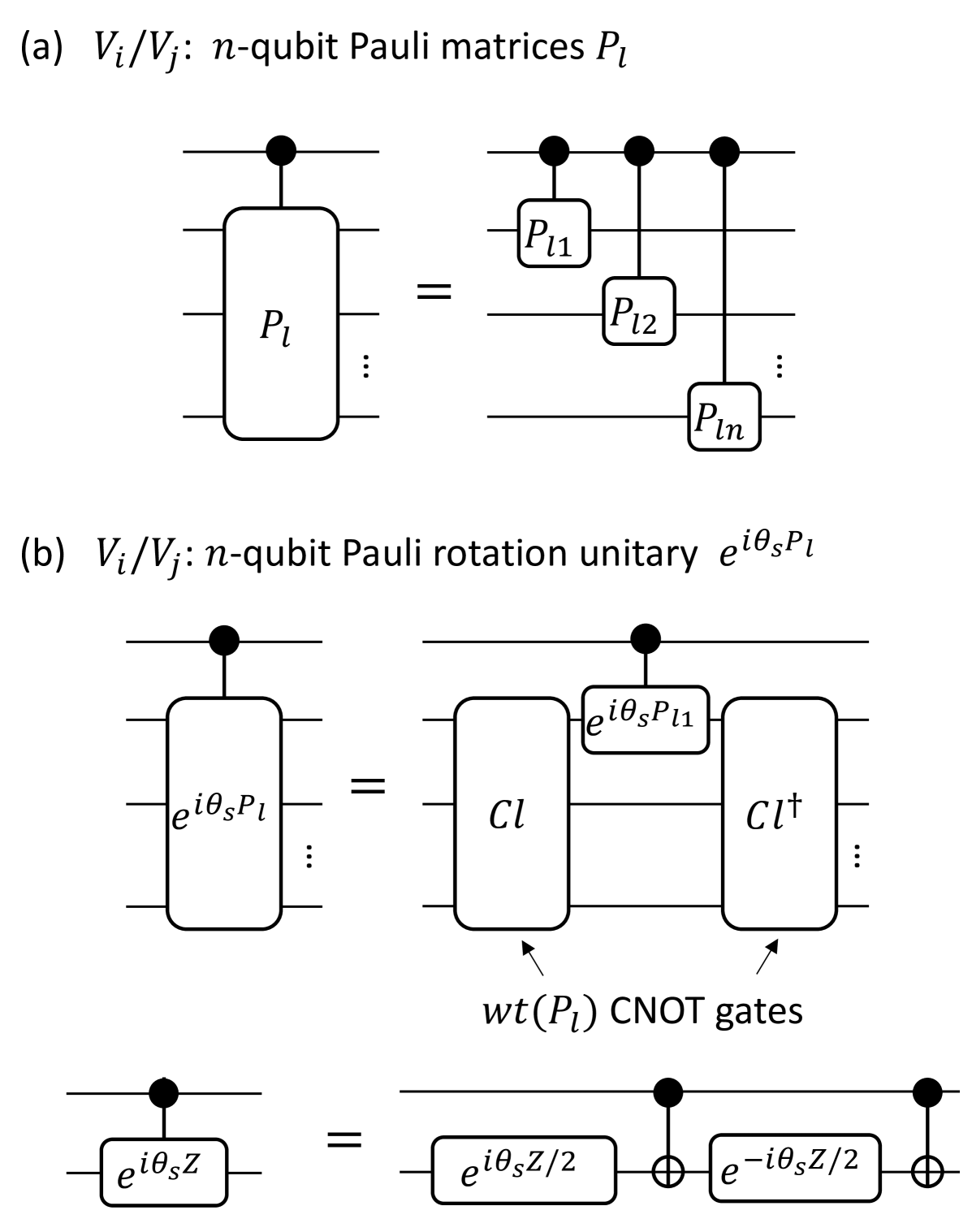
The gate complexity of the random-sampling implementation of the Trotter-LCU algorithm is determined by the segment number ν\nu, Trotter order KK and the gate complexity of each elementary gate in the LCU formula. As shown in Fig. 5, to construct controlled-U(t)U(t), we split it to ν\nu segments. In each segment, we need to implement KKth-order Trotter circuits and LCU circuits. The gate complexity of each elementary gate in the LCU circuit is determined by the truncation order scs_{c} of the Taylor-series compensation. Specifically, we consider the compilation of the controlled-Pauli gate and controlled-Pauli rotation gate, as shown in Fig. 11. The number of gates is determined by the weight of the sampled Pauli matrices wt(Pl)\mathrm{wt}(P_{l}), which is upper bounded by 𝒪(sc)\mathcal{O}(s_{c}).

Refer to caption
Figure 11: (a) Compilation of the LCU circuit when Vi(Vj)V_{i}(V_{j}) is a nn-qubit Pauli gate. (b) Compilation of the LCU circuit when Vi(Vj)V_{i}(V_{j}) is a Pauli rotation unitary. Here, ClCl is a Clifford gate with wt(Pl)\mathrm{wt}(P_{l}) 𝒞𝒩𝒪𝒯\mathcal{CNOT} gates.

Therefore, the gate complexity of the overall algorithm using KKth Trotter formula (K=0,1,2kK=0,1,2k) is given by

NK(RS)=𝒪(ν(κKL+sc))\displaystyle N_{K}^{(RS)}=\mathcal{O}(\nu(\kappa_{K}L+s_{c})) (86)

where

κK={0,K=0,1,K=1,2×5K/21,K=2k,k+.\kappa_{K}=\begin{cases}0,&K=0,\\ 1,&K=1,\\ 2\times 5^{K/2-1},&K=2k,k\in\mathbb{N}_{+}.\end{cases} (87)

Based on Eq. 86, the gate complexity of the 2k2kth-order Trotter-LCU algorithm is then

𝒪(ν(κKL+sc))=𝒪((λt)1+14k+1(κKL+log(1/ε)loglog(1/ε))).\mathcal{O}(\nu(\kappa_{K}L+s_{c}))=\mathcal{O}\left((\lambda t)^{1+\frac{1}{4k+1}}(\kappa_{K}L+\frac{\log(1/\varepsilon)}{\log\log(1/\varepsilon)})\right). (88)

Here, κK\kappa_{K} is the stage number of the Trotter formula. When K=0K=0, κK=0\kappa_{K}=0. When K=2kK=2k, κK=2×5K/21\kappa_{K}=2\times 5^{K/2-1}. ∎

From Theorem 1 we can see that, by introducing the LCU compensation, the time scaling of the KKth-order Trotter-LCU algorithm improve the bare KKth-order Trotter time scaling from 1+1/K1+1/K to 1+1/(2K+1)1+1/(2K+1). Moreover, the accuracy scaling is exponentially improved. This allowss us to achieve optimal gate complexity with lower-order Trotter implementation. For example, the time dependence of using first-order (respectively, second-order) Trotter formula can be improved from t2t^{2} (respectively, t1+1/2t^{1+1/2}) to t1+1/3t^{1+1/3} (respectively, t1+1/5t^{1+1/5}) by adding LCU compensation.

V TROTTER-LCU FORMULA WITH NESTED-COMMUTATOR COMPENSATION

In this section, we provide detailed construction of the nested-commutator compensation Trotter-LCU algorithms and the gate complexity analysis. We first sketch the procedure to derive the nested-commutator form LCU formula in subsection V.1. Then we construct the LCU formula of of the first-order Trotter remainder of the lattice Hamiltonians in subsection V.2 as an example. In subsection V.3, we describe the random-sampling implementation of the nested-commutator compensation algorithm and analyze its gate complexity.

V.1 Derivation of the nested-commutator formula

Our aim is to expand the LCU formula for the KKth-order Trotter remainder VK(x):=U(x)SK(x)V_{K}(x):=U(x)S_{K}(x)^{\dagger} (K=1K=1 or 2k2k, k+k\in\mathbb{N}_{+}) in the following form:

VK(x)=I+s=K+12K+1FK,s(nc)(x)+FK,𝓇𝓈(nc)(x),V_{K}(x)=I+\sum_{s=K+1}^{2K+1}F_{K,s}^{(nc)}(x)+F_{K,\mathcal{res}}^{(nc)}(x), (89)

where the leading-order terms FK,s(nc)(x)F_{K,s}^{(nc)}(x) are written as a summation of nested commutators. We will use the following lemma of the operator-valued differential equation.

Lemma 3 ((Lemma A.1 in Childs et al. (2021)).

Let H(x)H(x), R(x)R(x) be continuous operator-valued functions defined for xx\in\mathbb{R}. Then, the first-order differential equation

ddxW(x)=H(x)W(x)+R(x),W(0) known,\frac{d}{dx}W(x)=H(x)W(x)+R(x),\quad W(0)\text{ known}, (90)

has a unique solution given by

W(x)=𝒯exp(0x𝑑τH(τ))W(0)\displaystyle W(x)=\mathcal{T}\exp\left(\int_{0}^{x}d\tau H(\tau)\right)W(0) (91)
+0x𝑑τ1𝒯exp(τ1x𝑑τ2H(τ2))R(τ1).\displaystyle\quad+\int_{0}^{x}d\tau_{1}\mathcal{T}\exp\left(\int_{\tau_{1}}^{x}d\tau_{2}H(\tau_{2})\right)R(\tau_{1}).

Here, 𝒯\mathcal{T} is the time-ordering operator.

In Eq. 90, if we set W(x)W(x) to be the real-time evolution U(x)=eiHxU(x)=e^{-iHx}, we can find that H(x)=iHH(x)=-iH and R(x)=0R(x)=0. Therefore, R(x)R(x) reflects the derivation of W(x)W(x) from the exponential function. We are going to apply Lemma 3 to SK(x)S_{K}(x)^{\dagger}, i.e., we set W(x):=SK(x)W(x):=S_{K}(x)^{\dagger} and H(x)=iHH(x)=iH. The deviation of SK(x)S_{K}(x)^{\dagger} from U(x)=eixHU(x)^{\dagger}=e^{ixH} is characterized by the following function,

RK(x)=ddxSK(x)iHSK(x).R_{K}(x)=\frac{d}{dx}S_{K}(x)^{\dagger}-iHS_{K}(x)^{\dagger}. (92)

Applying Lemma 3, we have

SK(x)=eixH+0x𝑑τei(xτ)HRK(τ).S_{K}(x)^{\dagger}=e^{ixH}+\int_{0}^{x}d\tau e^{i(x-\tau)H}R_{K}(\tau). (93)

The Trotter remainder VK(x)V_{K}(x) can then be expressed as

VK(x)\displaystyle V_{K}(x) =U(x)SK(x)=I+0x𝑑τeiτHRK(τ)\displaystyle=U(x)S_{K}(x)^{\dagger}=I+\int_{0}^{x}d\tau e^{-i\tau H}R_{K}(\tau) (94)
=I+0x𝑑τU(τ)SK(τ)SK(τ)RK(τ)\displaystyle=I+\int_{0}^{x}d\tau U(\tau)S_{K}(\tau)^{\dagger}S_{K}(\tau)R_{K}(\tau)
=I+0x𝑑τVK(τ)JK(τ),\displaystyle=I+\int_{0}^{x}d\tau V_{K}(\tau)J_{K}(\tau),

where

JK(x):=SK(x)RK(x).J_{K}(x):=S_{K}(x)R_{K}(x). (95)

Eq. 94 provides a recurrence formula to solve the expansion terms in VK(x)V_{K}(x). To be more explicit, if we expand VK(x)V_{K}(x) and JK(x)J_{K}(x) based on the operator-valued Taylor series,

VK(x)=s=0Gsxss!,JK(x)=s=0Csxss!,V_{K}(x)=\sum_{s=0}^{\infty}G_{s}\frac{x^{s}}{s!},\quad J_{K}(x)=\sum_{s=0}^{\infty}C_{s}\frac{x^{s}}{s!}, (96)

where GsG_{s} and CsC_{s} denotes the respective ss-order term, then we have

Gs+1\displaystyle G_{s+1} =(s+1)!xs+10x𝑑τm=0sGmCsmτsm!(sm)!\displaystyle=\frac{(s+1)!}{x^{s+1}}\int_{0}^{x}d\tau\sum_{m=0}^{s}G_{m}C_{s-m}\frac{\tau^{s}}{m!(s-m)!} (97)
=m=0s(sm)GmCsm\displaystyle=\sum_{m=0}^{s}\binom{s}{m}G_{m}C_{s-m}

since Eq. 94 holds for all xx\in\mathbb{R}. This is a recurrence formula which can be used to solve all the expansion terms GsG_{s} of the remainder VK(x)V_{K}(x) from the expansion terms CrC_{r} of JK(x)J_{K}(x).

To solve the explicit form of GsG_{s}, we need to study the form of expansion terms {Cr}r=0s1\{C_{r}\}_{r=0}^{s-1} for the function JK(x)J_{K}(x). We will use the following proposition derived from Lemma 2.

Proposition 5 (Order condition).

For the KKth-order Trotter formula SK(x)S_{K}(x), the multiplicative remainder VK(x)V_{K}(x) and derivative remainder JK(x)J_{K}(x) defined in Eq. 89, Eq. 92 and Eq. 95, respectively, the following statements are equivalent.

  1. (1)

    SK(x)=U(x)+𝒪(xK+1)S_{K}(x)=U(x)+\mathcal{O}(x^{K+1}),

  2. (2)

    (SK(0))(j)=(iH)j(S_{K}(0))^{(j)}=(-iH)^{j}, for 0jK0\leq j\leq K,

  3. (3)

    JK(x)=𝒪(xK)J_{K}(x)=\mathcal{O}(x^{K}),

  4. (4)

    (JK(0))(j)=0(J_{K}(0))^{(j)}=0, for 0jK10\leq j\leq K-1,

  5. (5)

    VK(x)=I+𝒪(xK+1)V_{K}(x)=I+\mathcal{O}(x^{K+1}),

  6. (6)

    VK(0)=IV_{K}(0)=I and (VK(0))(j)=0(V_{K}(0))^{(j)}=0, for 1jK1\leq j\leq K.

Here, f(x)(j)f(x)^{(j)} is the jjth-derivative of the function f(x)f(x).

Proof.

First, we note that (1)(2)(1)\Leftrightarrow(2), (3)(4)(3)\Leftrightarrow(4), and (5)(6)(5)\Leftrightarrow(6) by applying Lemma 2 and setting F(x)F(x) to be SK(x)U(x)S_{K}(x)-U(x), JK(x)J_{K}(x), and VK(x)IV_{K}(x)-I, respectively. So we only need to prove (2)(4)(2)\Leftrightarrow(4) and (2)(6)(2)\Leftrightarrow(6).

We first prove (2)(4)(2)\Leftrightarrow(4). From (2)(2) we also have (SK(x))(j)=(iH)j(S_{K}(x)^{\dagger})^{(j)}=(iH)^{j} for 0jK0\leq j\leq K. Based on Eq. 92 and Eq. 95, the derivatives of RK(x)R_{K}(x) and JK(x)J_{K}(x) are

(RK(x))(j)\displaystyle(R_{K}(x))^{(j)} =(SK(x))(j+1)iH(SK(x))(j),\displaystyle=(S_{K}(x)^{\dagger})^{(j+1)}-iH(S_{K}(x)^{\dagger})^{(j)}, (98)
(JK(x))(j)\displaystyle(J_{K}(x))^{(j)} =l=0j(jl)(SK(x))(l)(RK(x))(jl).\displaystyle=\sum_{l=0}^{j}\binom{j}{l}(S_{K}(x))^{(l)}(R_{K}(x))^{(j-l)}.

Based on (2)(2) we have (RK(0))(j)=0(R_{K}(0))^{(j)}=0 for 0jK10\leq j\leq K-1. Hence (JK(0))(j)=0(J_{K}(0))^{(j)}=0 for 0jK10\leq j\leq K-1.

For the reverse direction, we notice that RK(x)=JK(x)SK(x)R_{K}(x)=J_{K}(x)S_{K}(x)^{\dagger}. This implies

(RK(x))(j)\displaystyle(R_{K}(x))^{(j)} =l=0j(jl)(JK(x))(l)(SK(x))(jl).\displaystyle=\sum_{l=0}^{j}\binom{j}{l}(J_{K}(x))^{(l)}(S_{K}(x)^{\dagger})^{(j-l)}. (99)

If we have (JK(0))(j)=0(J_{K}(0))^{(j)}=0 for 0jK10\leq j\leq K-1, then (RK(0))(j)=0(R_{K}(0))^{(j)}=0 for 0jK10\leq j\leq K-1. Then, from Eq. 98 we have (SK(x))(j)=(iH)j(S_{K}(x)^{\dagger})^{(j)}=(iH)^{j} for 0jK0\leq j\leq K, which is equivalent to (2)(2).

Now, we prove (2)(6)(2)\Leftrightarrow(6). Based on Eq. 89 we have

(VK(x))(j)=l=0j(jl)(U(x))(l)(SK(x))(jl).(V_{K}(x))^{(j)}=\sum_{l=0}^{j}\binom{j}{l}(U(x))^{(l)}(S_{K}(x)^{\dagger})^{(j-l)}. (100)

From (2)(2) we have

(VK(0))(j)=l=0j(jl)(iH)l(iH)jl=0,(V_{K}(0))^{(j)}=\sum_{l=0}^{j}\binom{j}{l}(-iH)^{l}(iH)^{j-l}=0, (101)

for 1<j<K1<j<K. The reverse direction can be proven similarly based on the derivative of the formula SK(x)=VK(x)U(x)S_{K}(x)=V_{K}(x)^{\dagger}U(x). ∎

From Proposition 5, we have the following order condition for the KKth-order Trotter formula and remainders,

SK(x)\displaystyle S_{K}(x) =U(x)+𝒪(xK+1),\displaystyle=U(x)+\mathcal{O}(x^{K+1}), (102)
JK(x)\displaystyle J_{K}(x) =𝒪(xK),\displaystyle=\mathcal{O}(x^{K}),
VK(x)\displaystyle V_{K}(x) =I+𝒪(xK+1).\displaystyle=I+\mathcal{O}(x^{K+1}).

Compare the recurrence formula in Eq. 94 and the order condition in Eq. 102, we will obtain the following relationship for the Taylor-series expansion terms GsG_{s} and CsC_{s} for VK(x)V_{K}(x) and JK(x)J_{K}(x), respectively,

Gs\displaystyle G_{s} =0,s=1,2,,K,\displaystyle=0,\quad s=1,2,.,K, (103)
Cs\displaystyle C_{s} =0,s=0,1,,K1,\displaystyle=0,\quad s=0,1,.,K-1,
Gs\displaystyle G_{s} =Cs1,s=K+1,K+2,,2K+1.\displaystyle=C_{s-1},\quad s=K+1,K+2,.,2K+1.

Based on Eq. 103, we are going to expand JK(x)J_{K}(x) based on the operator-valued Taylor-series expansion with integral remainders,

JK(x)=JK,L(x)+JK,res,2K(x)=s=K2KCsxss!+JK,res,2K(x),J_{K}(x)=J_{K,L}(x)+J_{K,res,2K}(x)=\sum_{s=K}^{2K}C_{s}\frac{x^{s}}{s!}+J_{K,res,2K}(x), (104)

where

Cs=JK(s)(0),s=K,K+1,,2K,\displaystyle C_{s}=J_{K}^{(s)}(0),\quad s=K,K+1,.,2K, (105)
JK,res,s(x)=0x𝑑τ(xτ)ss!JK(s+1)(τ).\displaystyle J_{K,res,s}(x)=\int_{0}^{x}d\tau\frac{(x-\tau)^{s}}{s!}J_{K}^{(s+1)}(\tau).

Here, JK,L(x):=s=K2KCsxss!J_{K,L}(x):=\sum_{s=K}^{2K}C_{s}\frac{x^{s}}{s!} denotes the leading-order terms in JK(x)J_{K}(x). Then, from Eq. 94 and Eq. 103, the KKth-order Trotter remainder can be expressed as

VK(x)\displaystyle V_{K}(x) =I+MK(x)=I+s=K+12K+1FK,s(nc)(x)+FK,𝓇𝓈(nc)(x),\displaystyle=I+M_{K}(x)=I+\sum_{s=K+1}^{2K+1}F_{K,s}^{(nc)}(x)+F_{K,\mathcal{res}}^{(nc)}(x), (106)
FK,s(nc)(x)\displaystyle F_{K,s}^{(nc)}(x) =Cs1xss!,s=K+1,K+2,,2K+1,\displaystyle=C_{s-1}\frac{x^{s}}{s!},\quad s=K+1,K+2,.,2K+1,
FK,𝓇𝓈(nc)(x)\displaystyle F_{K,\mathcal{res}}^{(nc)}(x) =0x𝑑τ(MK(τ)JK,L(τ)+VK(τ)JK,res,2K(τ)).\displaystyle=\int_{0}^{x}d\tau\left(M_{K}(\tau)J_{K,L}(\tau)+V_{K}(\tau)J_{K,res,2K}(\tau)\right).

Here, MK(x):=VK(x)IM_{K}(x):=V_{K}(x)-I.

From Eq. 106 we can see that, the leading-order expansion terms FK,s(nc)(x)F_{K,s}^{(nc)}(x) of VK(x)V_{K}(x) with s=K+1,K+2,,2K+1s=K+1,K+2,...,2K+1 owns a simple expression related to Cs1:=JK(s1)(0)C_{s-1}:=J_{K}^{(s-1)}(0). Later we will show that, CsC_{s} can be simply written as a summation of nested commutators with the form,

adHljmjadHl2m2adHl1m1Hl,\mathrm{ad}_{H_{l_{j}}}^{m_{j}}...\mathrm{ad}_{H_{l_{2}}}^{m_{2}}\mathrm{ad}_{H_{l_{1}}}^{m_{1}}H_{l}, (107)

where jmj=s\sum_{j}m_{j}=s, Hl,Hl1,,HljH_{l},H_{l_{1}},...,H_{l_{j}} are different summands in HH. Furthermore, we will show that {Cs}\{C_{s}\} are all anti-Hermitian. As a result, the expansion-order-pairing based on Euler’s formula introduced in Sec. IV can also be applied here. Since {Cs}\{C_{s}\} are anti-Hermitian, we can expand them by the Pauli operators as follows:

Cs=iCs1γPr(γ|s)Ps(nc)(γ),C_{s}=i\|C_{s}\|_{1}\sum_{\gamma}\Pr(\gamma|s)P^{(nc)}_{s}(\gamma), (108)

where {Ps(nc)(γ)}\{P^{(nc)}_{s}(\gamma)\} are Hermitian Pauli operators with coefficients 11 or 1-1. Cs1\|C_{s}\|_{1} denotes the 11-norm of this expansion. The leading-order expansion term FK,s(nc)(x)F_{K,s}^{(nc)}(x) can then be expressed as

FK,s(nc)(x)\displaystyle F_{K,s}^{(nc)}(x) =iCs11xss!γPr(γ|s1)Ps1(nc)(γ)\displaystyle=i\|C_{s-1}\|_{1}\frac{x^{s}}{s!}\sum_{\gamma}\Pr(\gamma|s-1)P^{(nc)}_{s-1}(\gamma) (109)
=:ηs(nc)VK,s(nc).\displaystyle=:\eta^{(nc)}_{s}V_{K,s}^{(nc)}.

Here, ηs(nc):=Cs11xss!\eta^{(nc)}_{s}:=\|C_{s-1}\|_{1}\frac{x^{s}}{s!} is the 11-norm of the LCU formula of FK,s(nc)(x)F_{K,s}^{(nc)}(x) in Eq. 109. VK,s(nc)V_{K,s}^{(nc)} is the normalized LCU formula.

The residue term FK,𝓇𝓈(nc)F_{K,\mathcal{res}}^{(nc)} in Eq. 106, however, is complicated and hard to be expressed simply using nested commutators. Due to the hardness to compensate FK,𝓇𝓈(nc)F_{K,\mathcal{res}}^{(nc)}, we will remove it in the truncated Trotter remainder formula,

V~K(nc)(x)=I+s=K+12K+1FK,s(nc)(x)\displaystyle\tilde{V}_{K}^{(nc)}(x)=I+\sum_{s=K+1}^{2K+1}F_{K,s}^{(nc)}(x) (110)
=s=K2Kηs(nc)ηΣ(nc)(I+ηΣ(nc)VK,s(nc))\displaystyle=\sum_{s=K}^{2K}\frac{\eta^{(nc)}_{s}}{\eta_{\Sigma}^{(nc)}}\left(I+\eta^{(nc)}_{\Sigma}V_{K,s}^{(nc)}\right)
=1+(ηΣ(nc))2s=K2Kηs(nc)ηΣ(nc)RK,s(nc)(ηΣ).\displaystyle=\sqrt{1+(\eta_{\Sigma}^{(nc)})^{2}}\sum_{s=K}^{2K}\frac{\eta^{(nc)}_{s}}{\eta_{\Sigma}^{(nc)}}R_{K,s}^{(nc)}(\eta_{\Sigma}).

Here, ηΣ(nc):=s=K+12K+1Cs11xss!\eta_{\Sigma}^{(nc)}:=\sum_{s=K+1}^{2K+1}\|C_{s-1}\|_{1}\frac{x^{s}}{s!}. In the fourth line, we apply the following pairing procedure based on Euler’s formula, similar to Eq. 75,

I+ηΣ(nc)VK,s(nc)=I+iηΣ(nc)γPr(γ|s1)Ps1(nc)(γ)\displaystyle I+\eta_{\Sigma}^{(nc)}V_{K,s}^{(nc)}=I+i\eta_{\Sigma}^{(nc)}\sum_{\gamma}\Pr(\gamma|s-1)P^{(nc)}_{s-1}(\gamma) (111)
=1+(ηΣ(nc))2γPr(γ|s1)exp(iθ(ηΣ(nc))Ps1(nc)(γ))\displaystyle=\sqrt{1+(\eta_{\Sigma}^{(nc)})^{2}}\sum_{\gamma}\Pr(\gamma|s-1)\exp\left(i\theta(\eta_{\Sigma}^{(nc)})P^{(nc)}_{s-1}(\gamma)\right)
=:1+(ηΣ(nc))2R2,s(nc)(ηΣ(nc)),\displaystyle=:\sqrt{1+(\eta_{\Sigma}^{(nc)})^{2}}R_{2,s}^{(nc)}(\eta_{\Sigma}^{(nc)}),

for s=K+1,K+2,,2K+1s=K+1,K+2,...,2K+1. Recall that θ(x):=tan1(x)\theta(x):=\tan^{-1}(x).

V~K(nc)(x)\tilde{V}_{K}^{(nc)}(x) in Eq. 110 is the final LCU formula for the nested-commutator compensation of VK(x)V_{K}(x). In what follows, we estimate the 11-norm μK(nc)(x)\mu_{K}^{(nc)}(x) and distance εK(nc)(x)\varepsilon_{K}^{(nc)}(x) of this LCU formula,

μK(nc)(x)\displaystyle\mu_{K}^{(nc)}(x) :=1+(ηΣ(nc))2,\displaystyle=\sqrt{1+(\eta_{\Sigma}^{(nc)})^{2}}, (112)
εK(nc)(x)\displaystyle\varepsilon_{K}^{(nc)}(x) :=V~K(nc)(x)VK(x)=FK,𝓇𝓈(nc)(x).\displaystyle=\|\tilde{V}_{K}^{(nc)}(x)-V_{K}(x)\|=\|F_{K,\mathcal{res}}^{(nc)}(x)\|.
Proposition 6 (Bound the 1-norm and error of nested-commutator expansion formula).

V~K(nc)(x)\tilde{V}^{(nc)}_{K}(x) in Eq. 110 is a (μK(nc)(x),εK(nc)(x))(\mu_{K}^{(nc)}(x),\varepsilon_{K}^{(nc)}(x)) formula of the KKth-order Trotter remainder VK(x)V_{K}(x) with

μK(nc)(x)\displaystyle\mu_{K}^{(nc)}(x) =1+(ηΣ(nc))2=1+(s=K2KCs1xs+1(s+1)!)2\displaystyle=\sqrt{1+(\eta_{\Sigma}^{(nc)})^{2}}=\sqrt{1+\left(\sum_{s=K}^{2K}\|C_{s}\|_{1}\frac{x^{s+1}}{(s+1)!}\right)^{2}} (113)
εK(nc)(x)\displaystyle\varepsilon_{K}^{(nc)}(x) 0x𝑑τ(MK(τ)JK,L(τ)+JK,res,2K(τ)),\displaystyle\leq\int_{0}^{x}d\tau\left(\|M_{K}(\tau)\|\|J_{K,L}(\tau)\|+\|J_{K,res,2K}(\tau)\|\right),

where

JK,L(τ)\displaystyle\|J_{K,L}(\tau)\| s=K2KCsxs+1(s+1)!,\displaystyle\leq\sum_{s=K}^{2K}\|C_{s}\|\frac{x^{s+1}}{(s+1)!}, (114)
JK,res,2K(τ)\displaystyle\|J_{K,res,2K}(\tau)\| 0x𝑑τ(xτ)ss!JK(s+1)(τ),\displaystyle\leq\int_{0}^{x}d\tau\frac{(x-\tau)^{s}}{s!}\|J_{K}^{(s+1)}(\tau)\|,
MK(τ)\displaystyle\|M_{K}(\tau)\| 0τ𝑑τ10τ1𝑑τ2(τ1τ2)(K1)(K1)!JK(K)(τ2).\displaystyle\leq\int_{0}^{\tau}d\tau_{1}\int_{0}^{\tau_{1}}d\tau_{2}\frac{(\tau_{1}-\tau_{2})^{(K-1)}}{(K-1)!}\|J_{K}^{(K)}(\tau_{2})\|.
Proof.

The value of μK(nc)(x)\mu_{K}^{(nc)}(x) is derived based on Eq. 109 and Eq. 110. To calculate εK(nc)(x)\varepsilon_{K}^{(nc)}(x), we will use the following bound,

εK(nc)(x)=FK,𝓇𝓈(nc)(x)\displaystyle\varepsilon_{K}^{(nc)}(x)=\|F_{K,\mathcal{res}}^{(nc)}(x)\| (115)
0x𝑑τ(MK(τ)JK,L(τ)+VK(τ)JK,res,2K(τ))\displaystyle\leq\int_{0}^{x}d\tau\left(\|M_{K}(\tau)\|\|J_{K,L}(\tau)\|+\|V_{K}(\tau)\|\|J_{K,res,2K}(\tau)\|\right)
=0x𝑑τ(MK(τ)JK,L(τ)+JK,res,2K(τ)).\displaystyle=\int_{0}^{x}d\tau\left(\|M_{K}(\tau)\|\|J_{K,L}(\tau)\|+\|J_{K,res,2K}(\tau)\|\right).

In the second equality, we use the fact that VK(τ)V_{K}(\tau) is a unitary. To bound JK,L(τ)\|J_{K,L}(\tau)\|, we have

JK,L(τ)s=K2KCsxs+1(s+1)!.\|J_{K,L}(\tau)\|\leq\sum_{s=K}^{2K}\|C_{s}\|\frac{x^{s+1}}{(s+1)!}. (116)

To bound JK,res,2K(τ)J_{K,res,2K}(\tau) in Eq. 115, from Eq. 105 we have

JK,res,2K(τ)0x𝑑τ(xτ)ss!JK(s+1)(τ).\|J_{K,res,2K}(\tau)\|\leq\int_{0}^{x}d\tau\frac{(x-\tau)^{s}}{s!}\|J_{K}^{(s+1)(\tau)}\|. (117)

Finally, to bound MK(τ)\|M_{K}(\tau)\| in Eq. 115, we have

MK(τ)\displaystyle\|M_{K}(\tau)\| =0τ𝑑τ1VK(τ1)JK(τ1)\displaystyle=\left\|\int_{0}^{\tau}d\tau_{1}V_{K}(\tau_{1})J_{K}(\tau_{1})\right\| (118)
0τ𝑑τ1JK(τ1)=0τ𝑑τ1JK,res,K1(τ1)\displaystyle\leq\int_{0}^{\tau}d\tau_{1}\|J_{K}(\tau_{1})\|=\int_{0}^{\tau}d\tau_{1}\|J_{K,res,K-1}(\tau_{1})\|
0τ𝑑τ10τ1𝑑τ2(τ1τ2)(K1)(K1)!JK(K)(τ2).\displaystyle\leq\int_{0}^{\tau}d\tau_{1}\int_{0}^{\tau_{1}}d\tau_{2}\frac{(\tau_{1}-\tau_{2})^{(K-1)}}{(K-1)!}\|J_{K}^{(K)}(\tau_{2})\|.

In the first line, we use the definition of MK(τ)=VK(τ)IM_{K}(\tau)=V_{K}(\tau)-I and the recurrence formula in Eq. 94. In the second line, we use the property that VK(τ)V_{K}(\tau) is a unitary. In the third line, we use the order condition in Proposition 5. In the final line, we apply the operator-valued Taylor-series expansion on JK(τ)J_{K}(\tau) and set the truncation order sc=K1s_{c}=K-1.

From Proposition 6 we can see that, to study the performance of the truncated LCU formula V~K(nc)(x)\tilde{V}^{(nc)}_{K}(x) in Eq. 110, we only need to study the property of the derivatives of JK(x)J_{K}(x), including {Cs}\{C_{s}\}. In the following section, we are going to derive the explicit formula of V~K(nc)(x)\tilde{V}^{(nc)}_{K}(x), taking the lattice Hamiltonian with first-order Trotter formulas as an example.

V.2 Example: first-order lattice Hamiltonian

Now, we focus on the lattice Hamiltonians with the form H=A+BH=A+B in Eq. 10. For the lattice Hamiltonian, the first-order Trotter formula is S1(x)=eixBeixAS_{1}(x)=e^{-ixB}e^{-ixA}. Here, we assume that the time-evolution of each two-qubit component eixHj,j+1e^{-ixH_{j,j+1}} is easy to be implement on the quantum computer.

To derive the explicit form of the LCU formula V~1(nc)(x)\tilde{V}_{1}^{(nc)}(x) in Eq. 110, we first derive J1(x)J_{1}(x) defined in Eq. 95 and its derivatives Cs:=J1(s)(x)C_{s}:=J_{1}^{(s)}(x). From Eq. 92 and Eq. 95 we have

R1(x)\displaystyle R_{1}(x) =ddxS1(x)iHS1(x)=i[eixA,B]eixB,\displaystyle=\frac{d}{dx}S_{1}(x)^{\dagger}-iHS_{1}(x)^{\dagger}=i[e^{ixA},B]e^{ixB}, (119)
J1(x)\displaystyle J_{1}(x) =S1(x)R1(x)=ieixBeixA[eixA,B]eixB\displaystyle=S_{1}(x)R_{1}(x)=ie^{-ixB}e^{-ixA}[e^{ixA},B]e^{ixB}
=i(BeixadBeixadAB).\displaystyle=i\left(B-e^{-ix\mathrm{ad}_{B}}e^{-ix\mathrm{ad}_{A}}B\right).

Applying the general Libniz formula to J1(x)J_{1}(x) we have,

J1(s)(x)=(i)s+1m1,n1;m1+n1=s(sm1)eixadBadBm1eixadAadAn1B.J_{1}^{(s)}(x)=(-i)^{s+1}\sum_{\begin{subarray}{c}m_{1},n_{1};\\ m_{1}+n_{1}=s\end{subarray}}\binom{s}{m_{1}}e^{-ix\mathrm{ad}_{B}}\mathrm{ad}_{B}^{m_{1}}e^{-ix\mathrm{ad}_{A}}\mathrm{ad}_{A}^{n_{1}}B. (120)

If we set the truncation of J1(s)(x)J_{1}^{(s)}(x) to be scs_{c} and apply the following operator Taylor-series expansion formula,

Q(x)=s=0scxss!Q(s)(0)+0x𝑑τ(xτ)scsc!Q(sc+1)(τ),Q(x)=\sum_{s=0}^{s_{c}}\frac{x^{s}}{s!}Q^{(s)}(0)+\int_{0}^{x}d\tau\frac{(x-\tau)^{s_{c}}}{s_{c}!}Q^{(s_{c}+1)}(\tau), (121)

we can expand J1(x)J_{1}(x) as

J1(x)=s=0scCsxss!+J1,𝓇𝓈(x),J_{1}(x)=\sum_{s=0}^{s_{c}}C_{s}\frac{x^{s}}{s!}+J_{1,\mathcal{res}}(x), (122)

where

Cs=J1(s)(0)\displaystyle C_{s}=J_{1}^{(s)}(0) =(i)s+1m1,n1;m1+n1=s(sm1)adBm1adAn1B,\displaystyle=(-i)^{s+1}\sum_{\begin{subarray}{c}m_{1},n_{1};\\ m_{1}+n_{1}=s\end{subarray}}\binom{s}{m_{1}}\mathrm{ad}_{B}^{m_{1}}\mathrm{ad}_{A}^{n_{1}}B, (123)
J1,res,sc(x)\displaystyle J_{1,res,s_{c}}(x) =0x𝑑τ(xτ)scsc!J1(sc+1)(τ).\displaystyle=\int_{0}^{x}d\tau\frac{(x-\tau)^{s_{c}}}{s_{c}!}J_{1}^{(s_{c}+1)}(\tau).

We can see that, CsC_{s} can be written as the summation of nested commutators with concise form adBm1adAn1B\mathrm{ad}_{B}^{m_{1}}\mathrm{ad}_{A}^{n_{1}}B. Note that, (i)s+1adBm1adAn1B(-i)^{s+1}\mathrm{ad}_{B}^{m_{1}}\mathrm{ad}_{A}^{n_{1}}B with m1+n1=sm_{1}+n_{1}=s is always anti-Hermitian when AA and BB are Hermitian. On the other hand, these nested commutators are all with the nice property that their spectral norm and 11-norm is linear to the system size nn. To be more specific, we have the following norm bound.

Proposition 7.

Consider a lattice Hamiltonian H=A+BH=A+B with the form in Eq. 10. Suppose the spectral norm and 11-norm of its components Hj,j+1H_{j,j+1} are upper bounded by Λ\Lambda and Λ1\Lambda_{1}. Then for the nested commutators appearing in Eq. 123, we have the following bound

eiτadBadBm1eiτadAadAn1Bn23m12n12sΛs+1,\displaystyle\left\|e^{-i\tau\mathrm{ad}_{B}}\mathrm{ad}_{B}^{m_{1}}e^{-i\tau\mathrm{ad}_{A}}\mathrm{ad}_{A}^{n_{1}}B\right\|\leq\frac{n}{2}3^{m_{1}}2^{n_{1}}2^{s}\Lambda^{s+1}, (124)

where m1,n1m_{1},n_{1} are non-negative integers satisfying m1+n1=sm_{1}+n_{1}=s. As a result, we can bound the spectral norm of J1(s)J_{1}^{(s)} as J1(s)(x)n210sΛs+1\|J_{1}^{(s)}(x)\|\leq\frac{n}{2}10^{s}\Lambda^{s+1}. The 11-norm upper bound is to simply replace Λ\Lambda by Λ1\Lambda_{1}.

Proof.

We first focus on one Hamiltonian term Hj,j+1H_{j,j+1} contained in BB and bound the norm,

eiτadBadBm1eiτadAadAn1(Hj,j+1)3m12n12sΛs+1.\left\|e^{-i\tau\mathrm{ad}_{B}}\mathrm{ad}_{B}^{m_{1}}e^{-i\tau\mathrm{ad}_{A}}\mathrm{ad}_{A}^{n_{1}}(H_{j,j+1})\right\|\leq 3^{m_{1}}2^{n_{1}}2^{s}\Lambda^{s+1}. (125)

To do this, we are going to decompose commutator to the elementary nested commutators in the following form:

eiτadBadHjs,js+1adHjn1+1,jn1+1+1\displaystyle e^{-i\tau\mathrm{ad}_{B}}\mathrm{ad}_{H_{j_{s},j_{s}+1}}.\mathrm{ad}_{H_{j_{n_{1}+1},j_{n_{1}+1}+1}}\cdot (126)
eiτadAadHjn1,jn1+1adHj1,j1+1Hj,j+1,\displaystyle\;e^{-i\tau\mathrm{ad}_{A}}\mathrm{ad}_{H_{j_{n_{1}},j_{n_{1}}+1}}.\mathrm{ad}_{H_{j_{1},j_{1}+1}}H_{j,j+1},

where j1,j2,,jsj_{1},j_{2},...,j_{s} are the possible vertice’s indices. For each elementary nested commutator, the spectral norm can be easily bounded by (2Λ)sΛ(2\Lambda)^{s}\Lambda by simply expanding all the commutators and applying triangle inequality. Here, we use the property that the spectral norm of all the exponential operators with anti-Hermitian exponent is 11.

Now, we count the number of the possible elementary commutators with the form in Eq. 126. We will check the action of each adjoint operator adA\mathrm{ad}_{A} or adB\mathrm{ad}_{B} from the right to the left. For the first location, if we expand adA\mathrm{ad}_{A}, there will be only two possible elementary nonzero components, adHj1,j\mathrm{ad}_{H_{j-1,j}} and adHj+1,j+2\mathrm{ad}_{H_{j+1,j+2}}. If the next ad\mathrm{ad} is still adA\mathrm{ad}_{A}, the support will still be on the four qubits: j1,j,j+1j-1,j,j+1, and j+2j+2. As a result, there will still be only two possible components, adHj1,j\mathrm{ad}_{H_{j-1,j}} and adHj+1,j+2\mathrm{ad}_{H_{j+1,j+2}}. Similarly, the exponential operator eiτadAe^{-i\tau\mathrm{ad}_{A}} will not enlarge the support since one can expand it to the power of adA\mathrm{ad}_{A}. The support will be enlarged when adB\mathrm{ad}_{B} comes. In this layer, the support of the operator will be expanded to six qubits, and there will be three elementary components. The number of possible elementary commutators is then

3m12n1.3^{m_{1}}2^{n_{1}}. (127)

Combining the number of elementary nested commutators and the norm bound for each commutator and applying triangle inequality, we will obtain Eq. 125. Finally, in the operator BB, there are n2\frac{n}{2} possible summands. This finishes the proof of Eq. 124.

Now, we apply Eq. 124 to bound the norm of J1(s)(x)J_{1}^{(s)}(x). From Eq. 120 we have

J1(s)(x)\displaystyle\|J_{1}^{(s)}(x)\| m1,n1;m1+n1=s(sm1)eixadBadBm1eixadAadAn1B\displaystyle\leq\sum_{\begin{subarray}{c}m_{1},n_{1};\\ m_{1}+n_{1}=s\end{subarray}}\binom{s}{m_{1}}\|e^{-ix\mathrm{ad}_{B}}\mathrm{ad}_{B}^{m_{1}}e^{-ix\mathrm{ad}_{A}}\mathrm{ad}_{A}^{n_{1}}B\| (128)
n22sΛs+1m1,n1;m1+n1=s(sm1)3m12n1\displaystyle\leq\frac{n}{2}2^{s}\Lambda^{s+1}\sum_{\begin{subarray}{c}m_{1},n_{1};\\ m_{1}+n_{1}=s\end{subarray}}\binom{s}{m_{1}}3^{m_{1}}2^{n_{1}}
=n210sΛs+1.\displaystyle=\frac{n}{2}0^{s}\Lambda^{s+1}.

In the third line, we apply the binomial theorem.

Since 11-norm can be estimated based on the same logic by counting the number of elementary nested commutators and the 11-norm of each nest commutator, the derivation for the 11-norm is similar by replacing Λ\Lambda to Λ1\Lambda_{1}. ∎

As introduced in subsection V.1, when K=1K=1, we set F1,s(nc)(x)F_{1,s}^{(nc)}(x) with s=2,3s=2,3 to be the leading-order terms and set the truncation order sc=3s_{c}=3. That is, we only compensate the second- and third-order error using LCU methods. While we are not able to achieve the logarithmic accuracy similar to PTSC algorithms, we can achieve a high accuracy of 𝒪(ε1/3)\mathcal{O}(\varepsilon^{-1/3}), which is cubicly improved comparing to the bare first-order Trotter result 𝒪(ε1)\mathcal{O}(\varepsilon^{-1}).

Based on Eq. 110, the truncated nested-commutator LCU formula for V1(x)V_{1}(x) can be written as

V~1(x)\displaystyle\tilde{V}_{1}(x) =I+s=23F1,s(nc)(x),\displaystyle=I+\sum_{s=2}^{3}F_{1,s}^{(nc)}(x), (129)
=1+(ηΣ(nc))2s=23ηs(nc)ηΣ(nc)R1,s(nc)(ηΣ).\displaystyle=\sqrt{1+(\eta_{\Sigma}^{(nc)})^{2}}\sum_{s=2}^{3}\frac{\eta_{s}^{(nc)}}{\eta_{\Sigma}^{(nc)}}R_{1,s}^{(nc)}(\eta_{\Sigma}).

Here, ηΣ(nc):=s=23Cs11xss!\eta_{\Sigma}^{(nc)}:=\sum_{s=2}^{3}\|C_{s-1}\|_{1}\frac{x^{s}}{s!}. The explicit form of R1,s(nc)(ηΣ)R_{1,s}^{(nc)}(\eta_{\Sigma}) can be obtained by the definitions in Eq. 109, Eq. 111 and the Pauli operator decomposition based on the nested-commutator form in Eq. 123.

Combined with the deterministic first-order Trotter formula, the overall LCU formula for U(x)U(x) is

U~1(nc)(x)=V~1(nc)(x)S1(x).\displaystyle\tilde{U}_{1}^{(nc)}(x)=\tilde{V}_{1}^{(nc)}(x)S_{1}(x). (130)

Following Proposition 6 and Proposition 7, we can bound the 11-norm and error of the LCU formula in Eq. 129 and Eq. 130 as follows.

Proposition 8 (first-order Trotter-LCU formula by nested-commutator compensation for lattice Hamiltonians).

Consider a lattice Hamiltonian with the form in Eq. 10. For min{14Λ,320Λ1}>x>0\min\{\frac{1}{4\Lambda},\frac{3}{20\Lambda_{1}}\}>x>0, Eq. 129 is a (μ1(nc)(x),ε1(nc)(x))(\mu_{1}^{(nc)}(x),\varepsilon_{1}^{(nc)}(x))-LCU formula of V1(x)V_{1}(x) with

μ1(nc)(x)\displaystyle\mu_{1}^{(nc)}(x) exp(10n2(Λ1x)4),\displaystyle\leq\exp\left(10n^{2}(\Lambda_{1}x)^{4}\right), (131)
ε1(nc)(x)\displaystyle\varepsilon_{1}^{(nc)}(x) 15n2(Λx)4.\displaystyle\leq 5n^{2}(\Lambda x)^{4}.

As a result, U~1(nc)(x)\tilde{U}_{1}^{(nc)}(x) in Eq. 130 is a (μ1(nc)(x),ε1(nc)(x))(\mu_{1}^{(nc)}(x),\varepsilon_{1}^{(nc)}(x))-LCU formula of U(x)U(x). Here, Λ1\Lambda_{1} and Λ\Lambda are defined in Eq. 11.

Proof.

We start from bounding the 11-norm μ1(nc)(x)\mu_{1}^{(nc)}(x). From Proposition 6 we have

μ1(nc)(x)\displaystyle\mu_{1}^{(nc)}(x) 1+(s=12Cs1xs+1(s+1)!)2\displaystyle\leq\sqrt{1+\left(\sum_{s=1}^{2}\|C_{s}\|_{1}\frac{x^{s+1}}{(s+1)!}\right)^{2}} (132)
1+12(s=12Cs1xs+1(s+1)!)2\displaystyle\leq 1+\frac{1}{2}\left(\sum_{s=1}^{2}\|C_{s}\|_{1}\frac{x^{s+1}}{(s+1)!}\right)^{2}
=1+n2(258(Λ1x)4+25012(Λ1x)5+12503!3!(Λ1x)6)\displaystyle=1+n^{2}\left(\frac{25}{8}(\Lambda_{1}x)^{4}+\frac{250}{12}(\Lambda_{1}x)^{5}+\frac{1250}{3!3!}(\Lambda_{1}x)^{6}\right)
1+3n2258(Λ1x)4exp(10n2(Λ1x)4).\displaystyle\leq 1+3n^{2}\frac{25}{8}(\Lambda_{1}x)^{4}\leq\exp\left(10n^{2}(\Lambda_{1}x)^{4}\right).

In the third line, we use the fact that Cs=J1(s)(0)C_{s}=J_{1}^{(s)}(0) and Proposition 7. In the fourth line, we use the assumption that Λ1x320\Lambda_{1}x\leq\frac{3}{20}.

Now, we bound the spectral norm distance ε1(nc)(x)=F1,𝓇𝓈(nc)\varepsilon_{1}^{(nc)}(x)=\|F_{1,\mathcal{res}}^{(nc)}\|. From Proposition 6 we know that we only need to bound J1,L(τ)\|J_{1,L}(\tau)\|, J1,res,2(τ)\|J_{1,res,2}(\tau)\|, and M1(τ)M_{1}(\tau) based on Eq. 114. For J1,L(τ)\|J_{1,L}(\tau)\|, from Proposition 7 we have

J1,L(τ)\displaystyle\|J_{1,L}(\tau)\| s=12Csτss!n2s=1210sΛs+1τss!.\displaystyle\leq\sum_{s=1}^{2}\|C_{s}\|\frac{\tau^{s}}{s!}\leq\frac{n}{2}\sum_{s=1}^{2}0^{s}\Lambda^{s+1}\frac{\tau^{s}}{s!}. (133)

For J1,res,2(τ)\|J_{1,res,2}(\tau)\| and M1(τ)\|M_{1}(\tau)\|, from Eq. 114 and Proposition 7 we have

J1,res,2(τ)\displaystyle\|J_{1,res,2}(\tau)\| 0τ𝑑τ1(ττ1)22!J1(3)(τ1)\displaystyle\leq\int_{0}^{\tau}d\tau_{1}\frac{(\tau-\tau_{1})^{2}}{2!}\|J_{1}^{(3)}(\tau_{1})\| (134)
n2103Λ4τ33!,\displaystyle\leq\frac{n}{2}0^{3}\Lambda^{4}\frac{\tau^{3}}{3!},
M1(τ)\displaystyle\|M_{1}(\tau)\| 0τ𝑑τ10τ1𝑑τ2J1(1)(τ2)\displaystyle\leq\int_{0}^{\tau}d\tau_{1}\int_{0}^{\tau_{1}}d\tau_{2}\|J_{1}^{(1)}(\tau_{2})\|
n210Λ2τ22!.\displaystyle\leq\frac{n}{2}0\Lambda^{2}\frac{\tau^{2}}{2!}.

Based on Eq. 133, Eq. 134 and Proposition 6,

F1,𝓇𝓈(nc)\displaystyle\|F_{1,\mathcal{res}}^{(nc)}\| 0x𝑑τ(M1(τ)J1,L(τ)+J1,res,2(τ))\displaystyle\leq\int_{0}^{x}d\tau\left(\|M_{1}(\tau)\|\|J_{1,L}(\tau)\|+\|J_{1,res,2}(\tau)\|\right) (135)
0x𝑑τ(n24s=1210s+1Λs+3τs+2s!2!+n2103Λ4τ33!)\displaystyle\leq\int_{0}^{x}d\tau\left(\frac{n^{2}}{4}\sum_{s=1}^{2}10^{s+1}\Lambda^{s+3}\frac{\tau^{s+2}}{s!2!}+\frac{n}{2}10^{3}\Lambda^{4}\frac{\tau^{3}}{3!}\right)
=n24s=1210s+1(Λx)s+2s!2!(s+3)+n2103(Λx)44!\displaystyle=\frac{n^{2}}{4}\sum_{s=1}^{2}0^{s+1}\frac{(\Lambda x)^{s+2}}{s!2!(s+3)}+\frac{n}{2}0^{3}\frac{(\Lambda x)^{4}}{4!}
2n24102(Λx)48+n2103(Λx)44!\displaystyle\leq 2\cdot\frac{n^{2}}{4}0^{2}\frac{(\Lambda x)^{4}}{8}+\frac{n}{2}0^{3}\frac{(\Lambda x)^{4}}{4!}
15n2(Λx)4.\displaystyle\leq 5n^{2}(\Lambda x)^{4}.

In the fourth line, we use the assumption that x14Λx\leq\frac{1}{4\Lambda}. ∎

V.3 General construction and performance

We can easily extend the first-order analysis above to the higher-order case. In Appendix B, we provide an explicit construction for second-order nested-commutator expansion, which will be used for the later numerical results. For the general LCU formula for the KKth-order Trotter remainder, we have the following proposition to characterize the LCU formulas V~K(x)\tilde{V}_{K}(x) in Eq. 110.

Proposition 9 (Trotter-LCU formula by nested-commutator compensation for lattice Hamiltonians).

Consider a lattice Hamiltonian with the form in Eq. 10. We set β:=2(4κ+5)\beta:=2(4\kappa+5) where κ\kappa is the stage number of the KKth-order Trotter formula (K=1K=1 or 2k2k). For min{K+1βΛ,K+2βΛ1}>x>0\min\{\frac{K+1}{\beta\Lambda},\frac{K+2}{\beta\Lambda_{1}}\}>x>0, V~K(nc)(x)\tilde{V}_{K}^{(nc)}(x) in Eq. 110 is a (μK(nc)(x),εK(nc)(x))(\mu_{K}^{(nc)}(x),\varepsilon_{K}^{(nc)}(x))-LCU formula of VK(x)V_{K}(x) with

μK(nc)\displaystyle\mu_{K}^{(nc)} exp(n2κ2β2(K+1)2(K!)2(Λ1x)2K+2),\displaystyle\leq\exp\left(\frac{n^{2}\kappa^{2}\beta^{2(K+1)}}{2(K!)^{2}}(\Lambda_{1}x)^{2K+2}\right), (136)
εK(nc)\displaystyle\varepsilon_{K}^{(nc)} (nκ)2β2K+1K!(K+1)!(Λx)2K+2.\displaystyle\leq(n\kappa)^{2}\frac{\beta^{2K+1}}{K!(K+1)!}(\Lambda x)^{2K+2}.

As a result, U~K(nc)(x)\tilde{U}_{K}^{(nc)}(x) in Eq. 110 is a (μK(nc)(x),εK(nc)(x))(\mu_{K}^{(nc)}(x),\varepsilon_{K}^{(nc)}(x))-LCU formula of U(x)U(x). Here, Λ\Lambda and Λ1\Lambda_{1} are, respectively, the largest spectral norm and 11-norm of the lattice Hamiltonian components defined in Eq. 11.

The proof of Proposition 9 is in Appendix C.

The circuit of random-sampling implementation of the NCC algorithm is similar to the PTSC algorithm, which is illustrated in Fig. 7. The only difference is that we sample the Pauli operators based on the nested-commutator expansion formula. In Appendix D, we generalize our random-sampling algorithm to the KKth-order situation to demonstrate its scalability. Specifically, the space and time cost of the sampling algorithm are 𝒪(KκK)\mathcal{O}(K\kappa_{K}) and 𝒪(K(logκK+logn))\mathcal{O}(K(\log{\kappa_{K}}+\log{n})), respectively. In practice, we need to expand the leading-order terms {FK,s}\{F_{K,s}\} to a summation of different adjoint operators based on the methods in subsection V.1 first, and then calculate the corresponding sampling probability Pr(γ|s)\Pr(\gamma|s). We have the following theorem to characterize the gate complexity of the KKth-order NCC algorithm with random-sampling implementation.

Theorem 2 (Gate complexity of the KKth-order random-sampling Trotter-LCU algorithm by nested-commutator compensation for lattice Hamiltonians).

In a KKth-order Trotter-LCU algorithm (K=1K=1 or 2k2k) based on nested-commutator compensation, if the segment number ν\nu satisfy all the requirements below,

ν\displaystyle\nu max{βΛK+1t,βΛ1K+2t},\displaystyle\geq\max\left\{\frac{\beta\Lambda}{K+1}t,\frac{\beta\Lambda_{1}}{K+2}t\right\}, (137)
ν\displaystyle\nu (κ22lnμ(K!)2)12K+1β1+12K+1n22K+1(Λ1t)1+12K+1,\displaystyle\geq\left(\frac{\kappa^{2}}{2\ln\mu(K!)^{2}}\right)^{\frac{1}{2K+1}}\beta^{1+\frac{1}{2K+1}}n^{\frac{2}{2K+1}}(\Lambda_{1}t)^{1+\frac{1}{2K+1}},
ν\displaystyle\nu (μκ2K!(K+1)!)12K+1βε12K+1n22K+1(Λt)1+12K+1,\displaystyle\geq\left(\frac{\mu\kappa^{2}}{K!(K+1)!}\right)^{\frac{1}{2K+1}}\beta\varepsilon^{-\frac{1}{2K+1}}n^{\frac{2}{2K+1}}(\Lambda t)^{1+\frac{1}{2K+1}},

we can then realize a (μ,ε)(\mu,\varepsilon)-LCU formula for U(t)U(t) based on ν\nu segments of U~K(nc)(x)\tilde{U}^{(nc)}_{K}(x) in Eq. 110. As a result, the gate complexity of random-sampling KKth-order Trotter-LCU algorithm based on nested-commutator compensation for the lattice Hamiltonian is

𝒪(n1+22K+1t1+12K+1ε12K+1).\mathcal{O}\left(n^{1+\frac{2}{2K+1}}t^{1+\frac{1}{2K+1}}\varepsilon^{-\frac{1}{2K+1}}\right). (138)

Here, β:=2(4κ+5)\beta:=2(4\kappa+5) where κ\kappa is the stage number of the Trotter formula. Λ\Lambda and Λ1\Lambda_{1} are, respectively, the largest spectral norm and 11-norm of the lattice Hamiltonian components defined in Eq. 11.

Proof.

For the random-sampling implementation, the overall LCU formula for U(t)U(t) is to repeat the sampling of U~K(nc)(x)\tilde{U}_{K}^{(nc)}(x) for ν\nu times, U~K,𝓉𝓉(nc)(t)=U~K(nc)(x)ν\tilde{U}_{K,\mathcal{tot}}^{(nc)}(t)=\tilde{U}_{K}^{(nc)}(x)^{\nu}. Using Proposition 2 and 9, when 0<x<min{K+1βΛ,K+2βΛ1}0<x<\min\{\frac{K+1}{\beta\Lambda},\frac{K+2}{\beta\Lambda_{1}}\}, we conclude that U~K,𝓉𝓉(nc)(t)\tilde{U}_{K,\mathcal{tot}}^{(nc)}(t) is a (μK,𝓉𝓉(nc)(t),ϵK,𝓉𝓉(nc)(t))(\mu_{K,\mathcal{tot}}^{(nc)}(t),\epsilon_{K,\mathcal{tot}}^{(nc)}(t))-LCU formula of U(t)U(t) with

μK,𝓉𝓉(nc)(t)=μK(x)νexp(n2κ2β2(K+1)2(K!)2(Λ1t)2K+2ν2K+1),\displaystyle\mu_{K,\mathcal{tot}}^{(nc)}(t)=\mu_{K}(x)^{\nu}\leq\exp\left(\frac{n^{2}\kappa^{2}\beta^{2(K+1)}}{2(K!)^{2}}\frac{(\Lambda_{1}t)^{2K+2}}{\nu^{2K+1}}\right), (139)
εK,𝓉𝓉(nc)(t)νμK,𝓉𝓉(nc)(t)εK(nc)(x)\displaystyle\varepsilon_{K,\mathcal{tot}}^{(nc)}(t)\leq\nu\mu_{K,\mathcal{tot}}^{(nc)}(t)\varepsilon_{K}^{(nc)}(x)
νμK,𝓉𝓉(nc)(t)((nκ)2β2K+1K!(K+1)!(Λt)2K+2ν2K+2).\displaystyle\quad\quad\leq\nu\mu_{K,\mathcal{tot}}^{(nc)}(t)\left((n\kappa)^{2}\frac{\beta^{2K+1}}{K!(K+1)!}\frac{(\Lambda t)^{2K+2}}{\nu^{2K+2}}\right).

To realize a (μ,ε)(\mu,\varepsilon)-LCU formula for U(t)U(t), we only need the segment number ν\nu satisfy all the requirements in Eq. 137. It suffices to choice

ν=𝒪(n22K+1t1+12K+1ε12K+1).\nu=\mathcal{O}\left(n^{\frac{2}{2K+1}}t^{1+\frac{1}{2K+1}}\varepsilon^{-\frac{1}{2K+1}}\right). (140)

Based on Eq. 86, the gate complexity of the KKth-order Trotter-LCU algorithm is then

𝒪(ν(κKL+sc))=𝒪(n1+22K+1t1+12K+1ε12K+1).\mathcal{O}(\nu(\kappa_{K}L+s_{c}))=\mathcal{O}\left(n^{1+\frac{2}{2K+1}}t^{1+\frac{1}{2K+1}}\varepsilon^{-\frac{1}{2K+1}}\right). (141)

Here we use the fact that sc=2K+1=𝒪(1)s_{c}=2K+1=\mathcal{O}(1) and L=𝒪(n)L=\mathcal{O}(n) for lattice Hamiltonians. ∎

So far, we have restricted our construction of the nested-commutator expansion to lattice Hamiltonians. In practice, various physical Hamiltonians, including those for the electronic structure of quantum materials Babbush et al. (2018a), quantum chemistry Hamiltonians Lee et al. (2021); Berry et al. (2019); von Burg et al. (2021) and power-law interaction Hamiltonians Childs et al. (2021), also possess sparse properties. As a result, the methods for the nested-commutator expansion of the Trotter remainder VK(x)V_{K}(x) introduced in subsection V.1 can also be applied to a general Hamiltonian HH.

In Appendix E, we discuss how to perform the nested-commutator expansion of VK(x)V_{K}(x) for general Hamiltonians, and discuss the performance of the resulting LCU formula in Proposition 13. We find that the 11-norm of the LCU formula based on nested-commutator expansion is closely related to the following nested commutator norm of the Hamiltonian H=l=1LHlH=\sum_{l=1}^{L}H_{l},

α~com(H):=ls+1=1Ll2=1L[Hls+1,[Hl2,Hl]]].\tilde{\alpha}_{\mathrm{com}}(H):=\sum_{l_{s+1}=1}^{L}...\sum_{l_{2}=1}^{L}\|[H_{l_{s+1}},...[H_{l_{2}},H_{l}]]...]\|. (142)

α~com(H)\tilde{\alpha}_{\mathrm{com}}(H) is originally defined in Ref. Childs et al. (2021) to analyze the performance of Trotter methods. In Ref. Childs et al. (2021), the authors estimate the values of αH(s)\alpha^{(s)}_{H} for typical Hamiltonian models like plane-wave-basis quantum chemistry models, kk-local Hamiltonian, and Hamiltonians with power-law interactions. Following similar estimation methods, we can also calculate α~com(H)\tilde{\alpha}_{\mathrm{com}}(H) for different models and consider their explicit nested-commutator expansions. We will leave the explicit evaluation of other typical Hamiltonians for a future work.

VI CONCLUSION AND OUTLOOK

We study the Hamiltonian simulation algorithms based on the composition of Trotter and LCU algorithms. In both theoretical and numerical studies, we show that the 0th-order paired Taylor-series compensation (PTSC) algorithm, 2k2kth-order PTSC algorithm and the 2k2kth-order nested-commutator compensation (NCC) algorithm enjoy different advantages and will be useful in different scenarios. Taking the nn-qubit lattice Hamiltonian as an example: the 0th-order PTSC algorithm performs the best when tt is small compared with nn and 1/ε1/\varepsilon; the 2k2kth-order PTSC algorithm performs the best when nn is small compared with tt and 1/ε1/\varepsilon; while the 2k2kth-order NC algorithm performs the best when 1/ε1/\varepsilon is small compared with nn and tt. In practice, with finite system size nn, simulation time tt and inverse accuracy 1/ε1/\varepsilon, we can think about a hybrid implementation of different algorithms. For example, when the sparsity LL of a given Hamiltonian is large, we can first split the Hamiltonian to two parts,

H=H1+H2=j=1L1Hj+k=L1+1LHk,H=H_{1}+H_{2}=\sum_{j=1}^{L_{1}}H_{j}+\sum_{k=L_{1}+1}^{L}H_{k}, (143)

where the summands in H1H_{1} are the few dominant terms with large coefficients. We can then perform second-order Trotter only for H1H_{1}, and use PTS to expand the remainder

V2(x;H1)=j1=L11eiHj1xeiHxj2=1L1eiHj2x.V_{2}(x;H_{1})=\prod_{j_{1}=L_{1}}^{1}e^{iH_{j_{1}}x}e^{-iHx}\prod_{j_{2}=1}^{L_{1}}e^{iH_{j_{2}}x}. (144)

If the number of dominant terms L1L_{1} is small, we can then reduce the LL dependence of the algorithm similar to 0th-order PTSC algorithm while keep the good tt-dependence of second-order PTSC algorithm. As another example, we can hybridize second-order PTSC and NCC algorithms: we apply the nested-commutator compensation for the leading-order terms (i.e., the terms with s=3,4s=3,4, and 55), and normal Taylor-series compensation for higher-order terms. In this case, we can find an optimal truncation location scs_{c} which fulfills the high simulation accuracy requirement and keeps the nested-commutator scaling for the leading-order compensation terms.

The design of Trotter-LCU algorithms is based on a series connection of Trotter and LCU algorithms. A similar composition method can also be exploited for other Hamiltonian simulation algorithms Hagan and Wiebe (2023). For example, we may replace the deterministic Trotter with the ones with random permutation Childs et al. (2019). Recently, Cho et al. Cho et al. (2024) consider similar idea to compensate the Trotter error using randomized unitary operators. Using anticommutative cancellation Zhao and Yuan (2021), we can further reduce the compensation terms.

Acknowledgements.
We thank Xiaoming Zhang, Xiao Yuan, Min-Hsiu Hsieh, Yuan Su, Kaiwen Gui, Ming Yuan, Senrui Chen, and Ying Li for helpful discussion and suggestions. We would like to especially thank Wenjun Yu for highlighting the validity of the variant where the ancillary qubit is measured and reset for each segment. P. Z.  and L. J. acknowledge support from the ARO MURI (W911NF-21-1-0325), AFOSR MURI (FA9550-19-1-0399, FA9550-21-1-0209), AFRL (FA8649-21-P-0781), NSF (OMA-1936118, ERC-1941583, OMA-2137642), NTT Research, and the Packard Foundation (2020-71479). J.S. would like to thank support from the Innovate UK (Project No.10075020) and support through Schmidt Sciences, LLC. Q. Z. acknowledges HKU Seed Fund for Basic Research for New Staff via Project No. 2201100596, Guangdong Natural Science Fund via Project No. 2023A1515012185, National Natural Science Foundation of China (NSFC) via Projects No. 12305030 and No. 12347104, Hong Kong Research Grant Council (RGC) via No. 27300823, No. N_HKU718/23, and No. R6010-23, Guangdong Provincial Quantum Science Strategic Initiative GDZX2200001.

Appendix A PAIRED TAYLOR-SERIES COMPENSATION WITH HIGHER-ORDER TROTTER FORMULAS

Following the same idea in subsection IV.2, we now generalize it to the case with 2k2kth-order Trotter formula. Expanding the 2k2kth-order Trotter remainder, we have

V2k(x)=s=0F2k,s(x)=s=0ηsV2k,s,V_{2k}(x)=\sum_{s=0}^{\infty}F_{2k,s}(x)=\sum_{s=0}^{\infty}\eta_{s}V_{2k,s}, (145)

where

F2k,s(x)\displaystyle F_{2k,s}(x) =ηsr,γPr(r,γ|s)P2k(r,γ),\displaystyle=\eta_{s}\sum_{r,\gamma}\Pr(r,\gamma|s)P_{2k}(r,\gamma), (146)
Pr(r,γ|s)\displaystyle\Pr(r,\gamma|s) :=Pr(r,r1:κ,r1:κ|s)l1:rpl1:r(r),\displaystyle=\Pr(r,\vec{r}_{1:\kappa},\vec{r}^{\prime}_{1:\kappa}|s)\sum_{l_{1:r}}p_{l_{1:r}}^{(r)},
P2k(r,γ)\displaystyle P_{2k}(r,\gamma) :=(i)2rsPrκPr1(Pl1:r(r))\displaystyle=(-i)^{2r-s}\prod^{\leftarrow}\vec{P}^{\vec{r}^{\prime}_{\kappa}}.\prod^{\leftarrow}\vec{P}^{\vec{r}^{\prime}_{1}}\left(P^{(r)}_{l_{1:r}}\right)\cdot
Pr1Prκ.\displaystyle\quad\prod^{\rightarrow}\vec{P}^{\vec{r}_{1}}.\prod^{\rightarrow}\vec{P}^{\vec{r}_{\kappa}}.

Here, we use γ\gamma to denote all the expansion variables {r1:κ,r1:κ,l1:r}\{\vec{r}_{1:\kappa},\vec{r}^{\prime}_{1:\kappa},l_{1:r}\} besides rr.

We ignore the derivation and provide the general form of the LCU formula for V~2k(p)(x)\tilde{V}_{2k}^{(p)}(x),

V~2k(p)(x)\displaystyle\tilde{V}_{2k}^{(p)}(x) =μ2k(p)(x)(s=2k+14k+1Pr2k(p)(s)R2k,s(p)(ηΣ)\displaystyle=\mu_{2k}^{(p)}(x)\Big{(}\sum_{s=2k+1}^{4k+1}\mathrm{Pr}_{2k}^{(p)}(s)R_{2k,s}^{(p)}(\eta_{\Sigma}) (147)
+s=4k+2scPr2k(p)(s)V2k,s(p)).\displaystyle\quad+\sum_{s=4k+2}^{s_{c}}\mathrm{Pr}_{2k}^{(p)}(s)V_{2k,s}^{(p)}\Big{)}.

where

μ2k(p)(x)\displaystyle\mu_{2k}^{(p)}(x) =1+(ηΣ)2+s=4k+2scηs,ηΣ=s=2k+14k+1ηs,\displaystyle=\sqrt{1+(\eta_{\Sigma})^{2}}+\sum_{s=4k+2}^{s_{c}}\eta_{s},\quad\eta_{\Sigma}=\sum_{s=2k+1}^{4k+1}\eta_{s}, (148)
Pr(p)(s)\displaystyle\mathrm{Pr}^{(p)}(s) =1μ2k(p)(x){1+(ηΣ)2ηsηΣ,s=2k+1,2k+2,,4k+1,ηs,s=4k+2,4k+3,,sc.\displaystyle=\frac{1}{\mu_{2k}^{(p)}(x)}\begin{cases}&\sqrt{1+(\eta_{\Sigma})^{2}}\frac{\eta_{s}}{\eta_{\Sigma}},\\ &\quad s=2k+1,2k+2,...,4k+1,\\ &\eta_{s},\\ &\quad s=4k+2,4k+3,...,s_{c}.\\ \end{cases}

The Pauli rotation unitary R2k,2q+1(p)(y):=exp(iθ(y)P2k(r,γ))R_{2k,2q+1}^{(p)}(y):=\exp(i\theta(y)P_{2k}^{\prime}(r,\gamma)^{\prime}) where θ(y):=tan1(1+y2)\theta(y):=\tan^{-1}(1+y^{2}) and P2k(r,γ):=(i)𝟙[P2k,s(r,γ):anti-Her]P2k(r,γ)P_{2k}^{\prime}(r,\gamma):=(-i)^{\mathbbm{1}[P_{2k,s}(r,\gamma):\text{anti-Her}]}P_{2k}(r,\gamma).

Combined with the deterministic Trotter formula, the overall LCU formula for U(x)U(x) is

U~2k(p)(x)=V~2k(p)(x)S2k(x).\displaystyle\tilde{U}_{2k}^{(p)}(x)=\tilde{V}_{2k}^{(p)}(x)S_{2k}(x). (149)

The following proposition gives the performance characterization of U~2k(p)(x)\tilde{U}_{2k}^{(p)}(x) to approximate U(x)U(x).

Proposition 10 (2k2kth-order Trotter-LCU formula by paired Taylor-series compensation).

For 0<x<1/(2λ)0<x<1/(2\lambda) and sc4k+1s_{c}\geq 4k+1, V~2k(p)(x)\tilde{V}_{2k}^{(p)}(x) in Eq. 147 is a (μ2k(p)(x),ε2k(p)(x))(\mu_{2k}^{(p)}(x),\varepsilon_{2k}^{(p)}(x))-LCU formula of V2k(x)V_{2k}(x) with

μ2k(p)(x)\displaystyle\mu_{2k}^{(p)}(x) e(e+ck)(2λx)4k+2,\displaystyle\leq e^{(e+c_{k})(2\lambda x)^{4k+2}}, (150)
ε2k(p)(x)\displaystyle\varepsilon_{2k}^{(p)}(x) (2eλxsc+1)sc+1.\displaystyle\leq\left(\frac{2e\lambda x}{s_{c}+1}\right)^{s_{c}+1}.

Here,

ck:=12(e2k+1)4k+2,c_{k}:=\frac{1}{2}\left(\frac{e}{2k+1}\right)^{4k+2}, (151)

so that 0.3>ck>00.3>c_{k}>0. As a result, U~2k(p)(x)\tilde{U}_{2k}^{(p)}(x) in Eq. 149 is a (μ2k(p)(x),ε2k(p)(x))(\mu_{2k}^{(p)}(x),\varepsilon_{2k}^{(p)}(x))-LCU formula of U(x)U(x).

Proof.

We will focus on the case with k=1k=1. The proof for a general kk is simiar. We first bound the normalization factor μ2(p)(x)\mu_{2}^{(p)}(x). When 2λx<12\lambda x<1 we have

μ2(p)(x)1+(ηΣ)2+s=6ηs\displaystyle\mu_{2}^{(p)}(x)\leq\sqrt{1+(\eta_{\Sigma})^{2}}+\sum_{s=6}^{\infty}\eta_{s}
1+12ηΣ2+(e2λxs=05ηs)\displaystyle\leq 1+\frac{1}{2}\eta_{\Sigma}^{2}+\left(e^{2\lambda x}-\sum_{s=0}^{5}\eta_{s}\right)
=12(2λx)6(13!+2λx4!+(2λx)25!)2+(e2λxs=15ηs)\displaystyle=\frac{1}{2}(2\lambda x)^{6}\left(\frac{1}{3!}+\frac{2\lambda x}{4!}+\frac{(2\lambda x)^{2}}{5!}\right)^{2}+\left(e^{2\lambda x}-\sum_{s=1}^{5}\eta_{s}\right) (152)
12(2λx)6(s=313!)2+(e2λxs=15ηs)\displaystyle\leq\frac{1}{2}(2\lambda x)^{6}\left(\sum_{s=3}^{\infty}\frac{1}{3!}\right)^{2}+\left(e^{2\lambda x}-\sum_{s=1}^{5}\eta_{s}\right)
12(e3)6(2λx)6+ee(2λx)6e(e+c1)(2λx)6.\displaystyle\leq\frac{1}{2}\left(\frac{e}{3}\right)^{6}(2\lambda x)^{6}+e^{e(2\lambda x)^{6}}\leq e^{(e+c_{1})(2\lambda x)^{6}}.

In the fifth line, we use Corollary 1.

The distance bound can be derived in the same manner as the one in Proposition 4. ∎

Appendix B TIGHT NESTED-COMMUTATOR ANALYSIS FOR SECOND-ORDER TROTTER-LCU ALGORITHM

We can easily extend the methods for the first-order analysis in subsection V.2 to the higher-order case. Taking the second-order case as an example, the second-order Trotter formula of the lattice Hamiltonian is S2(x)=eix2AeixBeix2AS_{2}(x)=e^{-i\frac{x}{2}A}e^{-ixB}e^{-i\frac{x}{2}A}.

To derive the explicit LCU formula V~2(nc)(x)\tilde{V}_{2}^{(nc)}(x) in Eq. 110, we first derive J2(x)J_{2}(x) defined in Eq. 95 and its derivatives Cs:=J2(s)(x)C_{s}:=J_{2}^{(s)}(x). From Eq. 92 and Eq. 95 we have

S2(x)\displaystyle S_{2}(x)^{\dagger} =eixH+0x𝑑τei(xτ)HR2(τ),\displaystyle=e^{ixH}+\int_{0}^{x}d\tau e^{i(x-\tau)H}R_{2}(\tau), (153)
R2(τ)\displaystyle R_{2}(\tau) =i[eix2A,B]eixBeix2A+i2[eix2AeixB,A]eix2A,\displaystyle=i[e^{i\frac{x}{2}A},B]e^{ixB}e^{i\frac{x}{2}A}+\frac{i}{2}[e^{i\frac{x}{2}A}e^{ixB},A]e^{i\frac{x}{2}A},
J2(x)\displaystyle J_{2}(x) =S2(x)R2(x)=i2(Aeix2adAeixadBA)\displaystyle=S_{2}(x)R_{2}(x)=\frac{i}{2}\left(A-e^{-i\frac{x}{2}\mathrm{ad}_{A}}e^{-ix\mathrm{ad}_{B}}A\right)
+i(eix2adABeix2adAeixadBeix2adAB).\displaystyle+i\left(e^{-i\frac{x}{2}\mathrm{ad}_{A}}B-e^{-i\frac{x}{2}\mathrm{ad}_{A}}e^{-ix\mathrm{ad}_{B}}e^{-i\frac{x}{2}\mathrm{ad}_{A}}B\right).

Following the approach in subsection V.1, we expand V2(x)V_{2}(x) and J2(x)J_{2}(x) by

V2(x)=s=0Gsxss!,J2(x)=s=0Csxss!,\displaystyle V_{2}(x)=\sum_{s=0}^{\infty}G_{s}\frac{x^{s}}{s!},\quad J_{2}(x)=\sum_{s=0}^{\infty}C_{s}\frac{x^{s}}{s!}, (154)

then based on Proposition 5 and the recurrence formula Eq. 94 we have,

G1=G2=0,C0=C1=0,\displaystyle G_{1}=G_{2}=0,\quad C_{0}=C_{1}=0, (155)
Gs=Cs1,s=3,4,5.\displaystyle G_{s}=C_{s-1},\quad s=3,4,5.

Combining Eq. 153 and Eq. 155, we can show that

Gs=𝒪(ns3).G_{s}=\mathcal{O}(n^{\lfloor\frac{s}{3}\rfloor}). (156)

Therefore, the first three nontrivial terms G3,G4,G5=𝒪(n)G_{3},G_{4},G_{5}=\mathcal{O}(n). These terms will be set as the leading-order terms.

Based on Eq. 155, we are going to expand JK(x)J_{K}(x) based on the operator-valued Taylor-series expansion with integral remainders,

J2(x)=J2,L(x)+J2,res,4(x)=s=24Csxss!+J2,res,4(x),J_{2}(x)=J_{2,L}(x)+J_{2,res,4}(x)=\sum_{s=2}^{4}C_{s}\frac{x^{s}}{s!}+J_{2,res,4}(x), (157)

where

Cs\displaystyle C_{s} =J2(s)(0),s=2,3,4,\displaystyle=J_{2}^{(s)}(0),\quad s=2,3,4, (158)
J2,res,s(x)\displaystyle J_{2,res,s}(x) =0x𝑑τ(xτ)ss!J2(s+1)(τ).\displaystyle=\int_{0}^{x}d\tau\frac{(x-\tau)^{s}}{s!}J_{2}^{(s+1)}(\tau).

J2,L(x):=s=24Csxss!J_{2,L}(x):=\sum_{s=2}^{4}C_{s}\frac{x^{s}}{s!} denotes the leading-order terms in JK(x)J_{K}(x). Then, from Eq. 94 and Eq. 155, the second-order Trotter remainder can be expressed as

V2(x)\displaystyle V_{2}(x) =I+s=35F2,s(nc)(x)+F2,𝓇𝓈(nc)(x),\displaystyle=I+\sum_{s=3}^{5}F_{2,s}^{(nc)}(x)+F_{2,\mathcal{res}}^{(nc)}(x), (159)
F2,s(nc)(x)\displaystyle F_{2,s}^{(nc)}(x) =Cs1xss!,3,4,5,\displaystyle=C_{s-1}\frac{x^{s}}{s!},\quad 3,4,5,
F2,𝓇𝓈(nc)(x)\displaystyle F_{2,\mathcal{res}}^{(nc)}(x) =0x𝑑τ(M2(τ)J2,L(τ)+V2(τ)J2,res,4(τ)).\displaystyle=\int_{0}^{x}d\tau\left(M_{2}(\tau)J_{2,L}(\tau)+V_{2}(\tau)J_{2,res,4}(\tau)\right).

We put the explicit nested-commutator expressions of the leading-order terms F2,s(nc)(x)F_{2,s}^{(nc)}(x) (s=3,4s=3,4, or 55) in Sec. B.

In practice, we truncate the formula with the order sc=5s_{c}=5. Based on Eq. 110, the truncated nested-commutator LCU formula for V2(x)V_{2}(x) can be written as

V~2(x)\displaystyle\tilde{V}_{2}(x) =I+s=35F2,s(nc)(x),\displaystyle=I+\sum_{s=3}^{5}F_{2,s}^{(nc)}(x), (160)
=1+(ηΣ(nc))2s=35ηs(nc)ηΣ(nc)R2,s(nc)(ηΣ).\displaystyle=\sqrt{1+(\eta_{\Sigma}^{(nc)})^{2}}\sum_{s=3}^{5}\frac{\eta_{s}^{(nc)}}{\eta_{\Sigma}^{(nc)}}R_{2,s}^{(nc)}(\eta_{\Sigma}).

Here, ηΣ(nc):=s=35Cs11xss!\eta_{\Sigma}^{(nc)}:=\sum_{s=3}^{5}\|C_{s-1}\|_{1}\frac{x^{s}}{s!}. The explicit form of R2,s(nc)(ηΣ)R_{2,s}^{(nc)}(\eta_{\Sigma}) can be obtained by the definitions in Eq. 109, Eq. 111 and the Pauli operator decomposition based on the nested-commutator form in Eq. 164.

For a tight numerical estimation, we seek for a tighter bound of the 11-norm μ2(nc)(x)\mu_{2}^{(nc)}(x) and spectral norm accuracy ε2(nc)(x)\varepsilon_{2}^{(nc)}(x) for the LCU formula in Eq. 160.

B.1 Bound the 1-norm of recurrence function

Hereafter, we define A:=i2AA^{\prime}:=-\frac{i}{2}A and B:=iBB^{\prime}:=-iB to simplify the notation. We have

J2(x)\displaystyle J_{2}(x) =Ja(x)+Jb(x),\displaystyle=J_{a}(x)+J_{b}(x), (161)
Ja(x)\displaystyle J_{a}(x) =(exadAexadBAA),\displaystyle=\left(e^{x\mathrm{ad}_{A^{\prime}}}e^{x\mathrm{ad}_{B^{\prime}}}A^{\prime}-A^{\prime}\right),
Jb(x)\displaystyle J_{b}(x) =(exadAexadBexadABexadAB).\displaystyle=\left(e^{x\mathrm{ad}_{A^{\prime}}}e^{x\mathrm{ad}_{B^{\prime}}}e^{x\mathrm{ad}_{A^{\prime}}}B^{\prime}-e^{x\mathrm{ad}_{A^{\prime}}}B^{\prime}\right).

Apply the Libniz rule to Ja(x)J_{a}(x) and Jb(x)J_{b}(x), we have

Ja(s)(x)\displaystyle J_{a}^{(s)}(x) =l=0s(sl)exadAadAlexadBadBslA,\displaystyle=\sum_{l=0}^{s}\binom{s}{l}e^{x\mathrm{ad}_{A^{\prime}}}\mathrm{ad}_{A^{\prime}}^{l}e^{x\mathrm{ad}_{B^{\prime}}}\mathrm{ad}_{B^{\prime}}^{s-l}A^{\prime}, (162)
Jb(s)(x)\displaystyle J_{b}^{(s)}(x) =l1,l2,l3l1+l2+l3=s,l2+l30(sl1,l2,l3)\displaystyle=\sum_{\begin{subarray}{c}l_{1},l_{2},l_{3}\\ l_{1}+l_{2}+l_{3}=s,l_{2}+l_{3}\neq 0\end{subarray}}\binom{s}{l_{1},l_{2},l_{3}}\cdot
exadAadAl1exadBadBl2exadAadAl3B.\displaystyle\quad\quad e^{x\mathrm{ad}_{A^{\prime}}}\mathrm{ad}_{A^{\prime}}^{l_{1}}e^{x\mathrm{ad}_{B^{\prime}}}\mathrm{ad}_{B^{\prime}}^{l_{2}}e^{x\mathrm{ad}_{A^{\prime}}}\mathrm{ad}_{A^{\prime}}^{l_{3}}B^{\prime}.

Then,

Cs\displaystyle C_{s} =l=0s1adAladBslA\displaystyle=\sum_{l=0}^{s-1}\mathrm{ad}_{A^{\prime}}^{l}\mathrm{ad}_{B^{\prime}}^{s-l}A (163)
+l1,l2,l3l1+l2+l3=s,l2+l30(sl1,l2,l3)adAl1adBl2adAl3B.\displaystyle\quad+\sum_{\begin{subarray}{c}l_{1},l_{2},l_{3}\\ l_{1}+l_{2}+l_{3}=s,l_{2}+l_{3}\neq 0\end{subarray}}\binom{s}{l_{1},l_{2},l_{3}}\mathrm{ad}_{A^{\prime}}^{l_{1}}\mathrm{ad}_{B^{\prime}}^{l_{2}}\mathrm{ad}_{A^{\prime}}^{l_{3}}B.

We can solve the explicit form of the leading-order terms with s=2,3s=2,3, and 44,

C2\displaystyle C_{2} =(adB2A+2adAadBA)+(3adA2B+2adBadAB),\displaystyle=\left(\mathrm{ad}_{B^{\prime}}^{2}A^{\prime}+2\mathrm{ad}_{A^{\prime}}\mathrm{ad}_{B^{\prime}}A^{\prime}\right)+\left(3\mathrm{ad}_{A^{\prime}}^{2}B^{\prime}+2\mathrm{ad}_{B^{\prime}}\mathrm{ad}_{A^{\prime}}B^{\prime}\right), (164)
C3\displaystyle C_{3} =(adB3A+3adAadB2A+3adA2adBA)+(7adA3B\displaystyle=\left(\mathrm{ad}_{B^{\prime}}^{3}A^{\prime}+3\mathrm{ad}_{A^{\prime}}\mathrm{ad}_{B^{\prime}}^{2}A^{\prime}+3\mathrm{ad}_{A^{\prime}}^{2}\mathrm{ad}_{B^{\prime}}A^{\prime}\right)+(7\mathrm{ad}_{A^{\prime}}^{3}B^{\prime}
+3adBadA2B+6adAadBadAB+3adB2adAB),\displaystyle\quad+3\mathrm{ad}_{B^{\prime}}\mathrm{ad}_{A^{\prime}}^{2}B^{\prime}+6\mathrm{ad}_{A^{\prime}}\mathrm{ad}_{B^{\prime}}\mathrm{ad}_{A^{\prime}}B^{\prime}+3\mathrm{ad}_{B^{\prime}}^{2}\mathrm{ad}_{A^{\prime}}B^{\prime}),
C4\displaystyle C_{4} =(adB4A+4adAadB3A+6adA2adB2A+4adA3adBA)\displaystyle=\left(\mathrm{ad}_{B^{\prime}}^{4}A^{\prime}+4\mathrm{ad}_{A^{\prime}}\mathrm{ad}_{B^{\prime}}^{3}A^{\prime}+6\mathrm{ad}_{A^{\prime}}^{2}\mathrm{ad}_{B^{\prime}}^{2}A^{\prime}+4\mathrm{ad}_{A^{\prime}}^{3}\mathrm{ad}_{B^{\prime}}A^{\prime}\right)
+(15adA4B+4adBadA3B+12adA2adBadAB\displaystyle\quad+(5\mathrm{ad}_{A^{\prime}}^{4}B^{\prime}+4\mathrm{ad}_{B^{\prime}}\mathrm{ad}_{A^{\prime}}^{3}B^{\prime}+2\mathrm{ad}_{A^{\prime}}^{2}\mathrm{ad}_{B^{\prime}}\mathrm{ad}_{A^{\prime}}B^{\prime}
+12adAadBadA2B+6adB2adA2B\displaystyle\quad+2\mathrm{ad}_{A^{\prime}}\mathrm{ad}_{B^{\prime}}\mathrm{ad}_{A^{\prime}}^{2}B^{\prime}+6\mathrm{ad}_{B^{\prime}}^{2}\mathrm{ad}_{A^{\prime}}^{2}B^{\prime}
+12adAadB2adAB+4adB3adAB).\displaystyle\quad+2\mathrm{ad}_{A^{\prime}}\mathrm{ad}_{B^{\prime}}^{2}\mathrm{ad}_{A^{\prime}}B^{\prime}+4\mathrm{ad}_{B^{\prime}}^{3}\mathrm{ad}_{A^{\prime}}B^{\prime}).

We can then expand the operators AA^{\prime} and BB^{\prime} to Pauli operators and solve the 11-norm of C2,C3C_{2},C_{3}, and C4C_{4} under the Pauli decomposition based on Eq. 164. The 11-norm of V~2(nc)(x)\tilde{V}_{2}^{(nc)}(x) is given by

μ~2(nc)(x)=1+(s=24Cs1xs+1(s+1)!)2.\tilde{\mu}_{2}^{(nc)}(x)=\sqrt{1+\left(\sum_{s=2}^{4}\|C_{s}\|_{1}\frac{x^{s+1}}{(s+1)!}\right)^{2}}. (165)

We summarize the procedure to estimate the segment number ν\nu of second-order Trotter-LCU under nested-commutator compensation as follows.

  1. 1.

    For a specific lattice Hamiltonian, get the explicit Pauli expansion form of C2C_{2}, C3C_{3}, C4C_{4} by Eq. 164.

  2. 2.

    Get the expression of the 11-norm μ~(nc)(x)\tilde{\mu}^{(nc)}(x) by Eq. 165. Calculate xUx_{U} based on μ~(nc)(x)=2\tilde{\mu}^{(nc)}(x)=2.

  3. 3.

    Solve the following residue operator,

    V2,𝓇𝓈(x)=V2(x)V~2(x)=U(x)S2(x),V_{2,\mathcal{res}}(x)=V_{2}(x)-\tilde{V}_{2}(x)=U(x)S_{2}(x)^{\dagger}, (166)

    calculate its spectral norm V2,𝓇𝓈(x)\|V_{2,\mathcal{res}}(x)\| numerically. Check either the following requirement are satisfied:

    V2,𝓇𝓈(x)txε,\|V_{2,\mathcal{res}}(x)\|\frac{t}{x}\leq\varepsilon, (167)

    where ε\varepsilon is a preset accuracy requirement. If not, we search the largest xx value in the region 0<x<xU0<x<x_{U} by dichotomy which makes Eq. 167 satisfied.

  4. 4.

    The number of segments is given by ν:=t/x\nu:=t/x. We then calculate the number of gates based on methods in Appendix B.2.

We have a tighter count bound for the norm of Ja(s)(x)J_{a}^{(s)}(x) and Jb(s)(x)J_{b}^{(s)}(x),

Proposition 11.

Consider a lattice Hamiltonian H=A+BH=A+B with the form in Eq. 10. Suppose the spectral norm and 11-norm of its components Hj,j+1H_{j,j+1} are bounded by Λ\Lambda and Λ1\Lambda_{1}. Then for the recurrence function J2(x)J_{2}(x), we have the following norm bound for its derivatives,

J2(s)(x)\displaystyle\|J^{(s)}_{2}(x)\| n2(7s+12s)Λs+1,\displaystyle\leq\frac{n}{2}(7^{s}+2^{s})\Lambda^{s+1}, (168)
J2(s)(x)1\displaystyle\|J^{(s)}_{2}(x)\|_{1} n2(7s+12s)Λ1s+1.\displaystyle\leq\frac{n}{2}(7^{s}+2^{s})\Lambda_{1}^{s+1}.
Proof.

From Eq. 162 we have,

Ja(s)(x)\displaystyle\|J_{a}^{(s)}(x)\| l=0s(sl)exadAadAlexadBadBslA,\displaystyle\leq\sum_{l=0}^{s}\binom{s}{l}\|e^{x\mathrm{ad}_{A^{\prime}}}\mathrm{ad}_{A^{\prime}}^{l}e^{x\mathrm{ad}_{B^{\prime}}}\mathrm{ad}_{B^{\prime}}^{s-l}A^{\prime}\|, (169)
Jb(s)(x)\displaystyle\|J_{b}^{(s)}(x)\| l1,l2,l3l1+l2+l3=s,l2+l30(sl1,l2,l3)\displaystyle\leq\sum_{\begin{subarray}{c}l_{1},l_{2},l_{3}\\ l_{1}+l_{2}+l_{3}=s,l_{2}+l_{3}\neq 0\end{subarray}}\binom{s}{l_{1},l_{2},l_{3}}\cdot
exadAadAl1exadBadBl2exadAadAl3B.\displaystyle\quad\|e^{x\mathrm{ad}_{A^{\prime}}}\mathrm{ad}_{A^{\prime}}^{l_{1}}e^{x\mathrm{ad}_{B^{\prime}}}\mathrm{ad}_{B^{\prime}}^{l_{2}}e^{x\mathrm{ad}_{A^{\prime}}}\mathrm{ad}_{A^{\prime}}^{l_{3}}B^{\prime}\|.

To bound the norm of nested commutators, we use the same methods in Proposition 7. We have

exadAadAlexadBadBslA\displaystyle\|e^{x\mathrm{ad}_{A^{\prime}}}\mathrm{ad}_{A^{\prime}}^{l}e^{x\mathrm{ad}_{B^{\prime}}}\mathrm{ad}_{B^{\prime}}^{s-l}A\| (170)
(3l2sl)(Λl(2Λ)sl)(n2Λ),\displaystyle\quad\quad\leq(3^{l}2^{s-l})(\Lambda^{l}(2\Lambda)^{s-l})\cdot(\frac{n}{2}\Lambda),
exadAadAl1exadBadBl2exadAadAl3B\displaystyle\|e^{x\mathrm{ad}_{A^{\prime}}}\mathrm{ad}_{A^{\prime}}^{l_{1}}e^{x\mathrm{ad}_{B^{\prime}}}\mathrm{ad}_{B^{\prime}}^{l_{2}}e^{x\mathrm{ad}_{A^{\prime}}}\mathrm{ad}_{A^{\prime}}^{l_{3}}B\|
(4l13l22l3)(Λl1(2Λ)l2Λl3)(n2Λ).\displaystyle\quad\quad\leq(4^{l_{1}}3^{l_{2}}2^{l_{3}})(\Lambda^{l_{1}}(2\Lambda)^{l_{2}}\Lambda^{l_{3}})\cdot(\frac{n}{2}\Lambda).

Here, the first bracket of each bound corresponds to possible nest commutators, while the second bracket of each bound indicates the norm enlargement of each nested commutator.

Combining Eq. 169 and Eq. 170, we have

Ja(s)(x)\displaystyle\|J_{a}^{(s)}(x)\| l=0s(sl)(3Λ)l(22Λ)sl)(n2Λ)\displaystyle\leq\sum_{l=0}^{s}\binom{s}{l}(3\Lambda)^{l}(2\cdot 2\Lambda)^{s-l})\cdot(\frac{n}{2}\Lambda) (171)
(7Λ)s(n2Λ),\displaystyle\leq(7\Lambda)^{s}\left(\frac{n}{2}\Lambda\right),
Jb(s)(x)\displaystyle\|J_{b}^{(s)}(x)\| l1,l2,l3l1+l2+l3=s,l2+l30(sl1,l2,l3)\displaystyle\leq\sum_{\begin{subarray}{c}l_{1},l_{2},l_{3}\\ l_{1}+l_{2}+l_{3}=s,l_{2}+l_{3}\neq 0\end{subarray}}\binom{s}{l_{1},l_{2},l_{3}}\cdot
(4Λ)l1(32Λ)l2(2Λ)l3)(n2Λ)\displaystyle\quad(4\Lambda)^{l_{1}}(3\cdot 2\Lambda)^{l_{2}}(2\Lambda)^{l_{3}})\cdot(\frac{n}{2}\Lambda)
(12Λ)s(n2Λ).\displaystyle\leq(2\Lambda)^{s}\left(\frac{n}{2}\Lambda\right).

The 11-norm bound can be derived in the same way. ∎

We can derive the bounds for μ~2(nc)(x)\tilde{\mu}_{2}^{(nc)}(x) and ε2(nc)(x)\varepsilon_{2}^{(nc)}(x) as follows:

μ~2(nc)(x)=1+(s=24Cs1xs+1(s+1)!)2\displaystyle\tilde{\mu}_{2}^{(nc)}(x)=\sqrt{1+\left(\sum_{s=2}^{4}\|C_{s}\|_{1}\frac{x^{s+1}}{(s+1)!}\right)^{2}} (172)
1+n24(s=24(7s+12s)(Λ1x)s+1(s+1)!)2\displaystyle\leq\sqrt{1+\frac{n^{2}}{4}\left(\sum_{s=2}^{4}(7^{s}+12^{s})\frac{(\Lambda_{1}x)^{s+1}}{(s+1)!}\right)^{2}} (173)
exp((35n)2(Λ1x)6),\displaystyle\leq\exp\left((35n)^{2}(\Lambda_{1}x)^{6}\right), (174)
ε2(nc)(x)n24(72+122)s=24(7s+12s)(Λx)s+43!s!(s+4)\displaystyle\varepsilon_{2}^{(nc)}(x)\leq\frac{n^{2}}{4}(7^{2}+12^{2})\sum_{s=2}^{4}(7^{s}+12^{s})\frac{(\Lambda x)^{s+4}}{3!s!(s+4)}
+n2(75+125)(Λx)66!\displaystyle\quad\quad\quad+\frac{n}{2}(7^{5}+12^{5})\frac{(\Lambda x)^{6}}{6!} (175)
(3n2+185n)(Λx)6370n2(Λx)6,\displaystyle\leq(3n^{2}+185n)(\Lambda x)^{6}\leq 370n^{2}(\Lambda x)^{6}, (176)

Here, Eq. 174 holds when Λ1x1/3\Lambda_{1}x\leq 1/3, Eq. 176 holds when Λx21/72\Lambda x\leq 21/72.

B.2 Estimating the gate counts

To estimate the performance, i.e., gate complexity of the Trotter-LCU algorithm based on nested-commutator compensation, we need to first estimate the number of segments ν=t/x\nu=t/x in the algorithm. This is determined by the following three constraints,

Λ1x,Λx1\displaystyle\Lambda_{1}x,\Lambda x\leq 1\quad\Leftarrow νmax{Λ1t,Λt},\displaystyle\nu\geq\max\{\Lambda_{1}t,\Lambda t\}, (177)
(μ~(nc))ν2\displaystyle(\tilde{\mu}^{(nc)})^{\nu}\leq 2\quad\Leftrightarrow νlnμ~(nc)ln2,\displaystyle\nu\ln\tilde{\mu}^{(nc)}\leq\ln 2,
νμ~ν(ε(nc))ε\displaystyle\nu\tilde{\mu}^{\nu}(\varepsilon^{(nc)})\leq\varepsilon\quad\Leftarrow νε(nc)12ε.\displaystyle\nu\varepsilon^{(nc)}\leq\frac{1}{2}\varepsilon.

After we solve the required segment number ν\nu by Eq. 177, we can estimate the gate number accordingly. Here, we introduce the method to estimate the gate number of the LCU part. The gate number in the implementation of second-order Trotter formula can be evaluated following the methods in Ref. Childs et al. (2018). In the worst-case scenario, the Pauli weight of the gate is determined by the weight of Pauli operators contained in C4C_{4} in Eq. 164. The largest Pauli weight is 66. As a result, a controlled-Pauli gate will cost at most six 𝒞𝒩𝒪𝒯\mathcal{CNOT} gates and no non-Clifford gate.

If we consider the paired algorithm, when we sample the third-order term, it will be a Pauli rotation unitary on four qubits. In this case, it will cost eight 𝒞𝒩𝒪𝒯\mathcal{CNOT} gates and two single-qubit Pauli rotation gates Rz(θ)R_{z}(\theta).

We summarize the whole procedure to estimate the gate complexity.

  1. 1.

    Input: Hamiltonian parameters: H=A+BH=A+B, nn, Λ\Lambda, Λ1\Lambda_{1}. Normalization requirements μ=2\mu=2, accuracy requirements ε\varepsilon, time requirements tt.

  2. 2.

    Normalization factor estimation.

    1. (a)

      Analytical way (scalable). Using Eq. 173 to get the function μ~(nc)(x)\tilde{\mu}^{(nc)}(x).

    2. (b)

      Numerical way (scalable). Using Eq. 164 to get the form of C2C_{2}, C3C_{3}, and C4C_{4}. Then get the function μ~(nc)(x)\tilde{\mu}^{(nc)}(x) by Eq. 172.

  3. 3.

    Accuracy estimation.

    1. (a)

      Analytical way (scalable). Using Eq. 175 to get the function ε(nc)(x)\varepsilon^{(nc)}(x).

    2. (b)

      Numerical way (unscalable). Calculate V2,𝓇𝓈(x):=U(x)S2(x)Is=24Csxs+1(s+1)!V_{2,\mathcal{res}}(x):=U(x)S_{2}(x)^{\dagger}-I-\sum_{s=2}^{4}C_{s}\frac{x^{s+1}}{(s+1)!} numerically. Solve its largest singular value, which is an upper bound of ε(nc)(x)\varepsilon^{(nc)}(x).

  4. 4.

    Based on the constraints in Eq. 177, calculate the segment number ν\nu.

  5. 5.

    Analyze the 𝒞𝒩𝒪𝒯\mathcal{CNOT} and Rz(θ)R_{z}(\theta) gate number.

Appendix C EXPLICIT NESTED-COMMUTATOR COMPENSATION FOR HIGHER-ORDER TROTTER REMAINDERS

In this section, we provide detailed results for the nested-commutator compensation for higher-order Trotter remainders introduced in Sec. V. Here, we will focus on the lattice model Hamiltonians in Eq. 10. The results for general Hamiltonians will be presented in Appendix E.

As introduced in Sec. V.1, for the (asymmetric) multiplicative remainder VK(x)V_{K}(x), our aim is to construct a LCU formula with the following form

VK(x)=I+s=K+12K+1FK,s(nc)(x)+FK,𝓇𝓈(nc)(x),V_{K}(x)=I+\sum_{s=K+1}^{2K+1}F_{K,s}^{(nc)}(x)+F_{K,\mathcal{res}}^{(nc)}(x), (178)

where FK,𝓇𝓈(nc)(x)F_{K,\mathcal{res}}^{(nc)}(x) denotes the term with xx-order 𝒪(x2K+2)\mathcal{O}(x^{2K+2}). In practice, we will use the truncated LCU formula with paired leading-order terms, derived in Eq. 110,

V~K(nc)(x)=I+s=K+12K+1FK,s(nc)(x)\displaystyle\tilde{V}_{K}^{(nc)}(x)=I+\sum_{s=K+1}^{2K+1}F_{K,s}^{(nc)}(x) (179)
=I+is=K2Kηs(nc)VK,s(nc)\displaystyle=I+i\sum_{s=K}^{2K}\eta^{(nc)}_{s}V_{K,s}^{(nc)}
=s=K2Kηs(nc)ηΣ(nc)(I+ηΣ(nc)VK,s(nc))\displaystyle=\sum_{s=K}^{2K}\frac{\eta^{(nc)}_{s}}{\eta_{\Sigma}^{(nc)}}\left(I+\eta^{(nc)}_{\Sigma}V_{K,s}^{(nc)}\right)
=1+(ηΣ(nc))2s=K2Kηs(nc)ηΣ(nc)RK,s(nc)(ηΣ),\displaystyle=\sqrt{1+(\eta_{\Sigma}^{(nc)})^{2}}\sum_{s=K}^{2K}\frac{\eta^{(nc)}_{s}}{\eta_{\Sigma}^{(nc)}}R_{K,s}^{(nc)}(\eta_{\Sigma}),

where ηΣ(nc)=s=K+12K+1ηs(nc)=s=K2KCs11xs+1(s+1)!\eta^{(nc)}_{\Sigma}=\sum_{s=K+1}^{2K+1}\eta^{(nc)}_{s}=\sum_{s=K}^{2K}\|C_{s-1}\|_{1}\frac{x^{s+1}}{(s+1)!}.

We are going to finish the following tasks,

  1. 1.

    (Sec. C.1) Derive the explicit formulas for the leading-order expansion terms FK,s(nc)(x)F_{K,s}^{(nc)}(x) with s=K+1,,2K+1s=K+1,...,2K+1.

  2. 2.

    (Sec. C.2) Prove the 11-norm μK(nc)(x)\mu_{K}^{(nc)}(x) and error bound εK(nc)(x)\varepsilon_{K}^{(nc)}(x) in Proposition 9.

C.1 Derivation of LCU formula with nested-commutator form

We first introduce the canonical expression of the KKth-order Trotter formula,

SK(x):=W(x)=j=1κWj(x)=Wκ(x)W2(x)W1(x),S_{K}(x):=W(x)=\prod_{j=1}^{\kappa}W_{j}(x)=W_{\kappa}(x)...W_{2}(x)W_{1}(x), (180)

where

Wj(x):=eixbjBeixajA,W_{j}(x):=e^{-ixb_{j}B}e^{-ixa_{j}A}, (181)

is the jjth stage of the Trotter formula. κ\kappa is the stage number. We have κ=1\kappa=1 for K=1K=1 and κ2×5k1\kappa\leq 2\times 5^{k-1} when K=2kK=2k. The stage lengths aja_{j} and bjb_{j} are determined based on Eq. 24 and Eq. 25. We have

0\displaystyle 0\leq aj,bj1,j=1,2,,κ,\displaystyle a_{j},b_{j}\leq 1,\quad\forall j=1,2,.,\kappa, (182)
j=1κ\displaystyle\sum_{j=1}^{\kappa} aj=j=1κbj=1.\displaystyle a_{j}=\sum_{j=1}^{\kappa}b_{j}=1.

For example, for the second-order Trotter formula S2(x)=eixA2eixBeixA2S_{2}(x)=e^{-ix\frac{A}{2}}e^{-ixB}e^{-ix\frac{A}{2}}, we set the stage number κ=2\kappa=2 with a1=12,b1=1;a2=12,b2=0a_{1}=\frac{1}{2},b_{1}=1;a_{2}=\frac{1}{2},b_{2}=0.

The Hermitian conjugate of W(x)W(x) is

W(x)=j=κ1Wj(x)=W1(x)W2(x)Wκ(x).W(x)^{\dagger}=\prod_{j=\kappa}^{1}W_{j}(x)^{\dagger}=W_{1}(x)^{\dagger}W_{2}(x)^{\dagger}...W_{\kappa}(x)^{\dagger}. (183)

As is discussed in Sec. V.1, to derive the nested-commutator form of VK(x)V_{K}(x), we first solve JK(x)J_{K}(x) defined in Eq. 95. We have

RK(x)\displaystyle R_{K}(x) =ddxW(x)iHW(x),\displaystyle=\frac{d}{dx}W(x)^{\dagger}-iHW(x)^{\dagger}, (184)
JK(x)\displaystyle J_{K}(x) :=W(x)RK(x).\displaystyle=W(x)R_{K}(x).

From Proposition 5, we can write the KKth-Trotter remainder VK(x)V_{K}(x) and JK(x)J_{K}(x) as the following form:

VK(x)\displaystyle V_{K}(x) :=I+MK(x)=I+s=K+12K+1Cs1xss!+FK,𝓇𝓈(x),\displaystyle=I+M_{K}(x)=I+\sum_{s=K+1}^{2K+1}C_{s-1}\frac{x^{s}}{s!}+F_{K,\mathcal{res}}(x), (185)
JK(x)\displaystyle J_{K}(x) =s=K2KCsxss!+JK,res,2K(x),\displaystyle=\sum_{s=K}^{2K}C_{s}\frac{x^{s}}{s!}+J_{K,res,2K}(x),

where FK,𝓇𝓈(x)=𝒪(x2K+2)F_{K,\mathcal{res}}(x)=\mathcal{O}(x^{2K+2}) and JK,res,2K(x)=𝒪(x2K+1)J_{K,res,2K}(x)=\mathcal{O}(x^{2K+1}) are the higher-order remaining terms to be analyzed later. We also denote

FL(x)\displaystyle F_{L}(x) :=s=K+12K+1Cs1xss!,\displaystyle=\sum_{s=K+1}^{2K+1}C_{s-1}\frac{x^{s}}{s!}, (186)
JL(x)\displaystyle J_{L}(x) :=s=K2KCsxss!,\displaystyle=\sum_{s=K}^{2K}C_{s}\frac{x^{s}}{s!},

as the leading-orders whose explicit forms will be calculated in this section. We will show that FL(x)F_{L}(x) contains 𝒪(n)\mathcal{O}(n) term where nn is the lattice size.

Now, we are going to solve the exact form of CsC_{s} for the leading-orders. We first try to solve the succinct form of RK(x)R_{K}(x) based on its definition in Eq. 184. Taking the derivative for each Trotter stage, we have

RK(x)=ddx[j=κ1Wj(x)]iHj=κ1Wj(x)\displaystyle R_{K}(x)=\frac{d}{dx}\left[\prod_{j=\kappa}^{1}W_{j}(x)^{\dagger}\right]-iH\prod_{j=\kappa}^{1}W_{j}(x)^{\dagger} (187)
=j=κ1l=j11Wl(x)ddxWj(x)l=κj+1Wl(x)\displaystyle=\sum_{j=\kappa}^{1}\prod_{l=j-1}^{1}W_{l}(x)^{\dagger}\frac{d}{dx}W_{j}(x)^{\dagger}\prod_{l=\kappa}^{j+1}W_{l}(x)^{\dagger}
j=κ1(iajA+ibjB)l=κ1Wl(x).\displaystyle\quad\quad-\sum_{j=\kappa}^{1}(ia_{j}A+ib_{j}B)\prod_{l=\kappa}^{1}W_{l}(x)^{\dagger}.

Here we assume 1j1<j+1κ1\leq j-1<j+1\leq\kappa. When j=1j=1 (or κ\kappa), the value of the product l=j11Wl(x)\prod_{l=j-1}^{1}W_{l}(x)^{\dagger} (or l=κj+1Wl(x)\prod_{l=\kappa}^{j+1}W_{l}(x)^{\dagger}) will be regarded as II. Recall that Wj(x)=eixajAeixbjBW_{j}(x)^{\dagger}=e^{ixa_{j}A}e^{ixb_{j}B}. We further expand ddxWj(x)\frac{d}{dx}W_{j}(x)^{\dagger} and merge the two terms together,

RK(x)=j=κ1l=j11Wl(x)(iajAWj(x)+Wj(x)ibjB)\displaystyle R_{K}(x)=\sum_{j=\kappa}^{1}\prod_{l=j-1}^{1}W_{l}(x)^{\dagger}\left(ia_{j}AW_{j}(x)^{\dagger}+W_{j}(x)^{\dagger}ib_{j}B\right)\cdot (188)
l=κj+1Wl(x)j=κ1(iajA+ibjB)l=κ1Wl(x)\displaystyle\quad\quad\prod_{l=\kappa}^{j+1}W_{l}(x)^{\dagger}-\sum_{j=\kappa}^{1}(ia_{j}A+ib_{j}B)\prod_{l=\kappa}^{1}W_{l}(x)^{\dagger}
=j=κ1[l=j1Wl(x),iaj+1A+ibjB]l=κj+1Wl(x).\displaystyle=\sum_{j=\kappa}^{1}\left[\prod_{l=j}^{1}W_{l}(x)^{\dagger},ia_{j+1}A+ib_{j}B\right]\prod_{l=\kappa}^{j+1}W_{l}(x)^{\dagger}.

Here, we assume aκ+1=0a_{\kappa+1}=0. Now, we simplify the commutator by splitting the product and then change the summation order,

RK(x)=j=κ1s=j1(m=s11Wm(x)[Ws(x),iaj+1A+ibjB]\displaystyle R_{K}(x)=\sum_{j=\kappa}^{1}\sum_{s=j}^{1}\Big{(}\prod_{m=s-1}^{1}W_{m}(x)^{\dagger}[W_{s}(x)^{\dagger},ia_{j+1}A+ib_{j}B]\cdot (189)
m=js+1Wm(x))l=κj+1Wl(x)\displaystyle\qquad\qquad\prod_{m=j}^{s+1}W_{m}(x)^{\dagger}\Big{)}\prod_{l=\kappa}^{j+1}W_{l}(x)^{\dagger}
=s=κ1j=κs(m=s11Wm(x)[Ws(x),iaj+1A+ibjB]\displaystyle=\sum_{s=\kappa}^{1}\sum_{j=\kappa}^{s}\Big{(}\prod_{m=s-1}^{1}W_{m}(x)^{\dagger}[W_{s}(x)^{\dagger},ia_{j+1}A+ib_{j}B]\cdot
m=js+1Wm(x))l=κj+1Wl(x)\displaystyle\qquad\qquad\prod_{m=j}^{s+1}W_{m}(x)^{\dagger}\Big{)}\prod_{l=\kappa}^{j+1}W_{l}(x)^{\dagger}
=s=κ1m=s11Wm(x)[Ws(x),icj+1A+idsB]l=κs+1Wl(x),\displaystyle=\sum_{s=\kappa}^{1}\prod_{m=s-1}^{1}W_{m}(x)^{\dagger}[W_{s}(x)^{\dagger},ic_{j+1}A+id_{s}B]\prod_{l=\kappa}^{s+1}W_{l}(x)^{\dagger},

where

cs:=j=κsaj,ds=j=κsbj,sκ.c_{s}:=\sum_{j=\kappa}^{s}a_{j},\quad d_{s}=\sum_{j=\kappa}^{s}b_{j},\quad s\leq\kappa. (190)

We also set cκ+1=0c_{\kappa+1}=0.

Based on Eq. 189, we now derive the succinct form of JK(x)J_{K}(x),

JK(x)=W(x)RK(x)=l=1κWl(x)RK(x)=s=κ1l=sκWl(x)[Ws(x),ics+1A+idsB]m=κs+1Wm(x).\displaystyle J_{K}(x)=W(x)R_{K}(x)=\prod_{l=1}^{\kappa}W_{l}(x)R_{K}(x)=\sum_{s=\kappa}^{1}\prod_{l=s}^{\kappa}W_{l}(x)[W_{s}(x)^{\dagger},ic_{s+1}A+id_{s}B]\prod_{m=\kappa}^{s+1}W_{m}(x)^{\dagger}. (191)

We expand each stage of the Trotter formula Wl(x)W_{l}(x) in the formula,

JK(x)\displaystyle J_{K}(x) =ij=κ1(l=j+1κWl(x)(cj+1A+djB)l=κj+1Wl(x)l=jκWl(x)(cj+1A+djB)l=κjWl(x))\displaystyle=i\sum_{j=\kappa}^{1}\left(\prod_{l=j+1}^{\kappa}W_{l}(x)^{\dagger}\left(c_{j+1}A+d_{j}B\right)\prod_{l=\kappa}^{j+1}W_{l}(x)^{\dagger}-\prod_{l=j}^{\kappa}W_{l}(x)^{\dagger}\left(c_{j+1}A+d_{j}B\right)\prod_{l=\kappa}^{j}W_{l}(x)^{\dagger}\right) (192)
=ij=κ1(l=jκeiτbladBeiτaladA(cj+1A+djB)l=j+1κeiτbladBeiτaladA(cj+1A+djB)).\displaystyle=-i\sum_{j=\kappa}^{1}\left(\prod_{l=j}^{\kappa}e^{-i\tau b_{l}\mathrm{ad}_{B}}e^{-i\tau a_{l}\mathrm{ad}_{A}}\left(c_{j+1}A+d_{j}B\right)-\prod_{l=j+1}^{\kappa}e^{-i\tau b_{l}\mathrm{ad}_{B}}e^{-i\tau a_{l}\mathrm{ad}_{A}}\left(c_{j+1}A+d_{j}B\right)\right).

Finally, we apply the following operator-valued Taylor expansion formula with integral form of the remainder:

Q(x)=s=0kxss!Q(s)(0)+0x𝑑τ(xτ)kk!Q(k+1)(τ).\displaystyle Q(x)=\sum_{s=0}^{k}\frac{x^{s}}{s!}Q^{(s)}(0)+\int_{0}^{x}d\tau\frac{(x-\tau)^{k}}{k!}Q^{(k+1)}(\tau). (193)

By the general Libniz formula, we obtain the derivatives of JK(x)J_{K}(x) as follows:

JK(s)(x)\displaystyle J^{(s)}_{K}(x) =(i)s+1j=κ1mj,nj;;mκ,nκmj,nj0;l=jκml+nl=s(smj,nj,,mκ,nκ)\displaystyle=(-i)^{s+1}\sum_{j=\kappa}^{1}\sum_{\begin{subarray}{c}m_{j},n_{j};...;m_{\kappa},n_{\kappa}\\ m_{j},n_{j}\neq 0;\sum_{l=j}^{\kappa}m_{l}+n_{l}=s\end{subarray}}\binom{s}{m_{j},n_{j},...,m_{\kappa},n_{\kappa}}\cdot (194)
l=jκ(blmlalnl)l=jκ(eixbladBadBmleixaladAadAnl)(cj+1A+djB).\displaystyle\quad\prod_{l=j}^{\kappa}(b_{l}^{m_{l}}a_{l}^{n_{l}})\prod_{l=j}^{\kappa}\left(e^{-ixb_{l}\mathrm{ad}_{B}}\mathrm{ad}_{B}^{m_{l}}e^{-ixa_{l}\mathrm{ad}_{A}}\mathrm{ad}_{A}^{n_{l}}\right)(c_{j+1}A+d_{j}B).

We can then expand JK(x)J_{K}(x) around t=0t=0 as follows:

JK(x)\displaystyle J_{K}(x) =s=K2KCsxss!+JK,res,2K(x).\displaystyle=\sum_{s=K}^{2K}C_{s}\frac{x^{s}}{s!}+J_{K,res,2K}(x). (195)

Here, we use the order condition in Proposition 5 so that the terms with expansion order from 0 to K1K-1 are all zeros. The ssth-order term CsC_{s} and the 2K2Kth-order residue JK,res,2K(x)J_{K,res,2K}(x) can then be expressed as

Cs\displaystyle C_{s} =JK(s)(0),\displaystyle=J^{(s)}_{K}(0), (196)
JK,res,2K(x)\displaystyle J_{K,res,2K}(x) =0x𝑑τ(xτ)2K(2K)!JK(2K+1)(τ).\displaystyle=\int_{0}^{x}d\tau\frac{(x-\tau)^{2K}}{(2K)!}J^{(2K+1)}_{K}(\tau).

C.2 Norm bounds for LCU formula

In Sec. C.1 we have derived the explicit form of the LCU formula for the KKth-order Trotter remainder VK(x)V_{K}(x). Based on Eq. 192, Eq. 194, Eq. 196 and Proposition 6, we are going to prove the 11-norm bound μK(nc)(x)\mu^{(nc)}_{K}(x) and error bound εK(nc)(x)\varepsilon^{(nc)}_{K}(x) in Proposition 9.

First of all, we need to estimate the norms of JK(s)(x)J_{K}^{(s)}(x). We have the following results.

Proposition 12 (Upper bound of the norm of nested commutators).

Consider a lattice Hamiltonian H=A+BH=A+B with the form in Eq. 10. Suppose the spectral norm and 11-norm of its components Hj,j+1H_{j,j+1} are bounded by Λ\Lambda and Λ1\Lambda_{1}. Then for the nested commutators appearing in Eq. 196, we have the following bound

l=jκeiτbladBadBmleiτaladAadAnl(cj+1A+djB)\displaystyle\left\|\prod_{l=j}^{\kappa}e^{-i\tau b_{l}\mathrm{ad}_{B}}\mathrm{ad}_{B}^{m_{l}}e^{-i\tau a_{l}\mathrm{ad}_{A}}\mathrm{ad}_{A}^{n_{l}}(c_{j+1}A+d_{j}B)\right\| (197)
n22sΛs+1(cj+1l=jκ(2(lj)+2)ml(2(lj)+1)nl\displaystyle\quad\leq\frac{n}{2}2^{s}\Lambda^{s+1}\Big{(}c_{j+1}\prod_{l=j}^{\kappa}(2(l-j)+2)^{m_{l}}(2(l-j)+1)^{n_{l}}
+djl=jκ(2(lj)+3)ml(2(lj)+2)nl)\displaystyle\quad\quad+d_{j}\prod_{l=j}^{\kappa}(2(l-j)+3)^{m_{l}}(2(l-j)+2)^{n_{l}}\Big{)}

where {ml,nl}l=1κ\{m_{l},n_{l}\}_{l=1}^{\kappa} are non-negative integers satisfying l=jκ(ml+nl)=s\sum_{l=j}^{\kappa}(m_{l}+n_{l})=s. κ\kappa is the stage number determined by the Trotter formula in Eq. 180. {al,bl}l=1κ\{a_{l},b_{l}\}_{l=1}^{\kappa} are defined by the Trotter formula in Eq. 181. {cl,dl}l=1κ\{c_{l},d_{l}\}_{l=1}^{\kappa} are defined in Eq. 190. As a result, we can bound the norm of JK(s)(x)J^{(s)}_{K}(x) defined in Eq. 194 as follows:

JK(s)(x)nκ(4κ+5)s2sΛs+1.\|J^{(s)}_{K}(x)\|\leq n\kappa(4\kappa+5)^{s}2^{s}\Lambda^{s+1}. (198)

The 11-norm upper bound for JK(s)(x)J^{(s)}_{K}(x) is to simply replace Λ\Lambda by Λ1\Lambda_{1}.

Proof.

To begin with, we now focus on one Hamiltonian term Hj,j+1H_{j,j+1} in AA and bound the norm

l=jκeiτbladBadBmleiτaladAadAnl(Hj,j+1)\displaystyle\left\|\prod_{l=j}^{\kappa}e^{-i\tau b_{l}\mathrm{ad}_{B}}\mathrm{ad}_{B}^{m_{l}}e^{-i\tau a_{l}\mathrm{ad}_{A}}\mathrm{ad}_{A}^{n_{l}}(H_{j,j+1})\right\| (199)
2sΛs+1l=jκ(2(lj)+2)ml(2(lj)+1)nl.\displaystyle\quad\leq 2^{s}\Lambda^{s+1}\prod_{l=j}^{\kappa}(2(l-j)+2)^{m_{l}}(2(l-j)+1)^{n_{l}}.

To this end, we decompose operator to the elementary nested commutators with the form,

eiτadBadHjs,js+1adHjsmκ+1,jsmκ+1+1\displaystyle e^{-i\tau\mathrm{ad}_{B}}\mathrm{ad}_{H_{j_{s},j_{s}+1}}.\mathrm{ad}_{H_{j_{s-m_{\kappa}+1},j_{s-m_{\kappa}+1}+1}}\cdot (200)
\displaystyle.
eiτadBadHjmj+nj,jmj+nj+1adHjnj+1,jnj+1+1\displaystyle e^{-i\tau\mathrm{ad}_{B}}\mathrm{ad}_{H_{j_{m_{j}+n_{j}},j_{m_{j}+n_{j}}+1}}.\mathrm{ad}_{H_{j_{n_{j}+1},j_{n_{j}+1}+1}}\cdot
eiτadAadHjnj,jnj+1adHj1,j1+1Hj,j+1,\displaystyle\;e^{-i\tau\mathrm{ad}_{A}}\mathrm{ad}_{H_{j_{n_{j}},j_{n_{j}}+1}}.\mathrm{ad}_{H_{j_{1},j_{1}+1}}H_{j,j+1},

where j1,j2,,jsj_{1},j_{2},...,j_{s} are the possible vertex indices. For each elementary nested commutator, the spectral norm can be bounded by

(2Λ)sΛ.(2\Lambda)^{s}\Lambda. (201)

This can he done by expand all the commutators and apply triangle inequality. Here, we use the property that the spectral norm of all the exponential operator with anti-Hermitian exponent is 1.

Now, we count the number of the possible elementary commutators with the form in Eq. 200. We will check the action of the adjoint operators from right to left. For the first location, we know that adAHj,j+1=0\mathrm{ad}_{A}H_{j,j+1}=0. For simplicity, we keep the term adHj,j+1Hj,j+1\mathrm{ad}_{H_{j,j+1}}H_{j,j+1} in the counting of elementary commutators. If the next ad\mathrm{ad} is still adA\mathrm{ad}_{A}, the support will still be on the two qubits jj and j+1j+1. As a result, there will be one possible elementary term adHj,j+1\mathrm{ad}_{H_{j,j+1}} left. Similarly, the exponential operator eiτadAe^{-i\tau\mathrm{ad}_{A}} will not enlarge the support since one can expand it to the power of adA\mathrm{ad}_{A}. The support will be enlarged when adB\mathrm{ad}_{B} comes into play. In this layer, the support of the operator will be expanded to four qubits: j1,j,j+1j-1,j,j+1, and j+2j+2. We can decompose adB\mathrm{ad}_{B} to 22 nonzero elementary elements, adHj1,j\mathrm{ad}_{H_{j-1,j}} and adHj+1,j+2\mathrm{ad}_{H_{j+1,j+2}}. If the next operator is still adB\mathrm{ad}_{B} or eiadBe^{-i\mathrm{ad}_{B}}, it will not enlarge the support. Following this logic, we can see that the number of possible elementary commutators is bounded by

(2(κj)+2)mκ(2(κj)+1)nκ4mj+13nj+12mj1nj\displaystyle(2(\kappa-j)+2)^{m_{\kappa}}(2(\kappa-j)+1)^{n_{\kappa}}.4^{m_{j+1}}3^{n_{j+1}}2^{m_{j}}1^{n_{j}} (202)
=l=jκ(2(lj)+2)ml(2(lj)+1)nl.\displaystyle\quad=\prod_{l=j}^{\kappa}(2(l-j)+2)^{m_{l}}(2(l-j)+1)^{n_{l}}.

We remark that, the elementary nested commutators with nj0n_{j}\neq 0 is actually 0. Here, we keep these commutators for the simplicity of counting.

Combining the number of elementary nested commutators and the norm bound for each commutator and applying triangle inequality, we will obtain Eq. 199.

Similarly, we can check one Hamiltonian term Hj,j+1H_{j,j+1} in BB and bound the norm with

l=jκeiτbladBadBmleiτaladAadAnl(Hj,j+1)\displaystyle\left\|\prod_{l=j}^{\kappa}e^{-i\tau b_{l}\mathrm{ad}_{B}}\mathrm{ad}_{B}^{m_{l}}e^{-i\tau a_{l}\mathrm{ad}_{A}}\mathrm{ad}_{A}^{n_{l}}(H_{j,j+1})\right\| (203)
2sΛs+1l=jκ(2(lj)+3)ml(2(lj)+2)nl.\displaystyle\quad\leq 2^{s}\Lambda^{s+1}\prod_{l=j}^{\kappa}(2(l-j)+3)^{m_{l}}(2(l-j)+2)^{n_{l}}.

The counting logic is similar to the case for Hj,j+1H_{j,j+1} in AA. The only difference is that when counting the number of elementary nested commutators, the action of the first adA\mathrm{ad}_{A} will enlarge the operator space to four qubits.

Applying Eq. 199 and Eq. 203 for all the components Hj,j+1H_{j,j+1} in HH, we will obtain Eq. 197.

Now, we apply Eq. 197 to bound the norm of JK(s)(x)J^{(s)}_{K}(x) in Eq. 194. We have

JK(s)(x)j=κ1mj,nj;;mκ,nκl=jκml+nl=s(smj,nj,,mκ,nκ)l=jκ(blmlalnl)l=jκ(eitbladBadBmleitaladAadAnl)(cj+1A+djB)\displaystyle\|J^{(s)}_{K}(x)\|\leq\sum_{j=\kappa}^{1}\sum_{\begin{subarray}{c}m_{j},n_{j};...;m_{\kappa},n_{\kappa}\\ \sum_{l=j}^{\kappa}m_{l}+n_{l}=s\end{subarray}}\binom{s}{m_{j},n_{j},...,m_{\kappa},n_{\kappa}}\prod_{l=j}^{\kappa}(b_{l}^{m_{l}}a_{l}^{n_{l}})\left\|\prod_{l=j}^{\kappa}\left(e^{-itb_{l}\mathrm{ad}_{B}}\mathrm{ad}_{B}^{m_{l}}e^{-ita_{l}\mathrm{ad}_{A}}\mathrm{ad}_{A}^{n_{l}}\right)(c_{j+1}A+d_{j}B)\right\|
2sΛs+1n2j=κ1mj,nj;;mκ,nκl=jκml+nl=s(smj,nj,,mκ,nκ)l=jκ(blmlalnl)\displaystyle\leq 2^{s}\Lambda^{s+1}\frac{n}{2}\sum_{j=\kappa}^{1}\sum_{\begin{subarray}{c}m_{j},n_{j};...;m_{\kappa},n_{\kappa}\\ \sum_{l=j}^{\kappa}m_{l}+n_{l}=s\end{subarray}}\binom{s}{m_{j},n_{j},...,m_{\kappa},n_{\kappa}}\prod_{l=j}^{\kappa}(b_{l}^{m_{l}}a_{l}^{n_{l}})
(cj+1l=jκ(2(lj)+2)ml(2(lj)+1)nl+djl=jκ(2(lj)+3)ml(2(lj)+2)nl)\displaystyle\quad\left(c_{j+1}\prod_{l=j}^{\kappa}(2(l-j)+2)^{m_{l}}(2(l-j)+1)^{n_{l}}+d_{j}\prod_{l=j}^{\kappa}(2(l-j)+3)^{m_{l}}(2(l-j)+2)^{n_{l}}\right)
2sΛs+1n2j=κ1cj+1(l=jκbl(2(lj)+2)+al(2(lj)+1))s+dj(l=jκbl(2(lj)+3)+al(2(lj)+2))s\displaystyle\leq 2^{s}\Lambda^{s+1}\frac{n}{2}\sum_{j=\kappa}^{1}c_{j+1}\left(\sum_{l=j}^{\kappa}b_{l}(2(l-j)+2)+a_{l}(2(l-j)+1)\right)^{s}+d_{j}\left(\sum_{l=j}^{\kappa}b_{l}(2(l-j)+3)+a_{l}(2(l-j)+2)\right)^{s}
2sΛs+1n2j=κ1cj+1(4(κj)+3)s+dj(4(κj)+5)s\displaystyle\leq 2^{s}\Lambda^{s+1}\frac{n}{2}\sum_{j=\kappa}^{1}c_{j+1}\left(4(\kappa-j)+3\right)^{s}+d_{j}\left(4(\kappa-j)+5\right)^{s} (204)
2sΛs+1n2j=κ1(4(κj)+3)s+(4(κj)+5)s\displaystyle\leq 2^{s}\Lambda^{s+1}\frac{n}{2}\sum_{j=\kappa}^{1}\left(4(\kappa-j)+3\right)^{s}+\left(4(\kappa-j)+5\right)^{s}
2sΛs+1n22κ(4κ+5)s=nκ(4κ+5)s2sΛs+1.\displaystyle\leq 2^{s}\Lambda^{s+1}\frac{n}{2}\cdot 2\kappa(4\kappa+5)^{s}=n\kappa(4\kappa+5)^{s}2^{s}\Lambda^{s+1}.

In the third line, we use multinomial theorem. In the fourth line, we use the fact that al,bl>0a_{l},b_{l}>0 and lal,lbl1\sum_{l}a_{l},\sum_{l}b_{l}\leq 1. The fifth line is due to 0cj,dj<10\leq c_{j},d_{j}<1 for all jj. In the sixth line, we use the following bound:

j=1κ(4(κj)+a)s=l=0κ1(4l+a)s\displaystyle\;\;\sum_{j=1}^{\kappa}(4(\kappa-j)+a)^{s}=\sum_{l=0}^{\kappa-1}(4l+a)^{s} (205)
0κ(4x+a)s𝑑x=14(4κ+a)s+1as+1s+1\displaystyle\leq\int_{0}^{\kappa}(4x+a)^{s}dx=\frac{1}{4}\frac{(4\kappa+a)^{s+1}-a^{s+1}}{s+1}
=κ1s+1m=0s(4κ+a)masmκ(4κ+a)s.\displaystyle=\kappa\frac{1}{s+1}\sum_{m=0}^{s}(4\kappa+a)^{m}a^{s-m}\leq\kappa(4\kappa+a)^{s}.

Here, aa is any real number.

Since 11-norm can be estimated based on the same logic by counting the number of nested commutators and the 11-norm of each nest commutator, the derivation for the 11-norm is similar by replacing Λ\Lambda to Λ1\Lambda_{1}.

Now, we prove the 11-norm bound μK(nc)(x)\mu^{(nc)}_{K}(x) of V~K(x)\tilde{V}_{K}(x). From Proposition 6 we have

V~K(x)1=1+(s=K2KCs1xs+1(s+1)!)2\displaystyle\|\tilde{V}_{K}(x)\|_{1}=\sqrt{1+\left(\sum_{s=K}^{2K}\|C_{s}\|_{1}\frac{x^{s+1}}{(s+1)!}\right)^{2}}
1+12(s=K2KCs1xs+1(s+1)!)2\displaystyle\leq 1+\frac{1}{2}\left(\sum_{s=K}^{2K}\|C_{s}\|_{1}\frac{x^{s+1}}{(s+1)!}\right)^{2}
1+12n2κ2(s=K2Kβs(Λ1x)s+1(s+1)!)2\displaystyle\leq 1+\frac{1}{2}n^{2}\kappa^{2}\left(\sum_{s=K}^{2K}\beta^{s}\frac{(\Lambda_{1}x)^{s+1}}{(s+1)!}\right)^{2} (206)
1+12n2κ2((K+1)βK+1(Λ1x)K+1(K+1)!)2\displaystyle\leq 1+\frac{1}{2}n^{2}\kappa^{2}\left((K+1)\beta^{K+1}\frac{(\Lambda_{1}x)^{K+1}}{(K+1)!}\right)^{2}
1+n2κ2β2(K+1)2(K!)2(Λ1x)2K+2\displaystyle\leq 1+\frac{n^{2}\kappa^{2}\beta^{2(K+1)}}{2(K!)^{2}}(\Lambda_{1}x)^{2K+2}
exp(n2κ2β2(K+1)2(K!)2(Λ1x)2K+2).\displaystyle\leq\exp\left(\frac{n^{2}\kappa^{2}\beta^{2(K+1)}}{2(K!)^{2}}(\Lambda_{1}x)^{2K+2}\right).

Here, we set β:=2(4κ+5)\beta:=2(4\kappa+5). In the third line, we use Proposition 12. In the fourth line, we use the assumption that βΛ1x(K+2)\beta\Lambda_{1}x\leq(K+2).

Then, we prove the distance bound εK(nc)(x)=FK,𝓇𝓈\varepsilon_{K}^{(nc)}(x)=\|F_{K,\mathcal{res}}\|. From Proposition 6 we know that we only need to bound JK,L(τ)\|J_{K,L}(\tau)\|, JK,res,2K(τ)\|J_{K,res,2K}(\tau)\|, and MK(τ)M_{K}(\tau) based on Eq. 114.

We start from JK,L(τ)\|J_{K,L}(\tau)\|. From Proposition 7 we have

JK,L(τ)\displaystyle\|J_{K,L}(\tau)\| s=K2KCsτss!\displaystyle\leq\sum_{s=K}^{2K}\|C_{s}\|\frac{\tau^{s}}{s!} (207)
nκs=K2KβsΛs+1τss!.\displaystyle\leq n\kappa\sum_{s=K}^{2K}\beta^{s}\Lambda^{s+1}\frac{\tau^{s}}{s!}.

Then, we bound JK,res,2K(τ)\|J_{K,res,2K}(\tau)\| and MK(τ)\|M_{K}(\tau)\|. From Eq. 114 and Proposition 12 we have

JK,res,2K(τ)\displaystyle\|J_{K,res,2K}(\tau)\| 0τ𝑑τ1(ττ1)2K(2K)!JK(2K+1)(τ1)\displaystyle\leq\int_{0}^{\tau}d\tau_{1}\frac{(\tau-\tau_{1})^{2K}}{(2K)!}\|J_{K}^{(2K+1)}(\tau_{1})\| (208)
nκ(βτ)2K+1(2K+1)!Λ2K+2,\displaystyle\leq n\kappa\frac{(\beta\tau)^{2K+1}}{(2K+1)!}\Lambda^{2K+2},
MK(τ)\displaystyle\|M_{K}(\tau)\| 0τ𝑑τ10τ1𝑑τ2(τ1τ2)(K1)(K1)!JK(K)(τ2)\displaystyle\leq\int_{0}^{\tau}d\tau_{1}\int_{0}^{\tau_{1}}d\tau_{2}\frac{(\tau_{1}-\tau_{2})^{(K-1)}}{(K-1)!}\|J_{K}^{(K)}(\tau_{2})\|
nκβKτK+1(K+1)!ΛK+1.\displaystyle\leq n\kappa\frac{\beta^{K}\tau^{K+1}}{(K+1)!}\Lambda^{K+1}.

Based on Eq. 207, Eq. 208 and Proposition 6 we have

FK,𝓇𝓈(x)0τ(MK(τ)JL(τ)+JK,res,2K(τ))\displaystyle\|F_{K,\mathcal{res}}(x)\|\leq\int_{0}^{\tau}\left(\|M_{K}(\tau)\|\|J_{L}(\tau)\|+\|J_{K,res,2K}(\tau)\|\right)
0x𝑑τ(nκ)2s=K2Kβs+KΛs+K+2τs+K+1(K+1)!s!\displaystyle\leq\int_{0}^{x}d\tau(n\kappa)^{2}\sum_{s=K}^{2K}\frac{\beta^{s+K}\Lambda^{s+K+2}\tau^{s+K+1}}{(K+1)!s!}
+(nκ)β2K+1Λ2K+2τ2K+1(2K+1)!\displaystyle\quad+(n\kappa)\frac{\beta^{2K+1}\Lambda^{2K+2}\tau^{2K+1}}{(2K+1)!} (209)
=(nκ)2s=K2Kβs+K(Λx)s+K+2(K+1)!s!(s+K+2)+(nκ)β2K+1(Λx)2K+2(2K+2)!\displaystyle=(n\kappa)^{2}\sum_{s=K}^{2K}\frac{\beta^{s+K}(\Lambda x)^{s+K+2}}{(K+1)!s!(s+K+2)}+(n\kappa)\frac{\beta^{2K+1}(\Lambda x)^{2K+2}}{(2K+2)!}
(nκ)2(K+1)β2K(Λx)2K+2(2K+2)K!(K+1)!+(nκ)β2K+1x2K+2(2K+2)!\displaystyle\leq(n\kappa)^{2}(K+1)\frac{\beta^{2K}(\Lambda x)^{2K+2}}{(2K+2)K!(K+1)!}+(n\kappa)\frac{\beta^{2K+1}x^{2K+2}}{(2K+2)!}
(nκ)2β2K+1K!(K+1)!(Λx)2K+2.\displaystyle\leq(n\kappa)^{2}\frac{\beta^{2K+1}}{K!(K+1)!}(\Lambda x)^{2K+2}.

In the fourth line, we assume βΛxK+1\beta\Lambda x\leq K+1. In the fifth line, we use the fact that nκ>1n\kappa>1.

To summarize, from Eq. 206 and Eq. 209, we have proven that,

μK(nc)\displaystyle\mu_{K}^{(nc)} :=VK(x)1exp(n2κ2β2(K+1)2(K!)2(Λ1x)2K+2),\displaystyle=\|V_{K}(x)\|_{1}\leq\exp\left(\frac{n^{2}\kappa^{2}\beta^{2(K+1)}}{2(K!)^{2}}(\Lambda_{1}x)^{2K+2}\right), (210)
εK(nc)\displaystyle\varepsilon_{K}^{(nc)} :=V~K(x)VK(x)=FK,𝓇𝓈(x)\displaystyle=\|\tilde{V}_{K}(x)-V_{K}(x)\|=\|F_{K,\mathcal{res}}(x)\|
(nκ)2β2K+1K!(K+1)!(Λx)2K+2.\displaystyle\leq(n\kappa)^{2}\frac{\beta^{2K+1}}{K!(K+1)!}(\Lambda x)^{2K+2}.

Here, β:=2(4κ+5)\beta:=2(4\kappa+5). We assume that βxmax{K+1Λ,K+2Λ1}\beta x\leq\max\{\frac{K+1}{\Lambda},\frac{K+2}{\Lambda_{1}}\}. This finish the proof of Proposition 9.

Appendix D EFFICIENT SAMPLING FOR THE HIGHER-ORDER NESTED-COMMUTATOR COMPENSATION ALGORITHM

Following the analysis in Appendix C, we now design a general sampling method for the general KKth-order Trotter remainder V~K(nc)(x)\tilde{V}_{K}^{(nc)}(x). We consider the general KKth-order Trotter formula in the canonical form in Eq. 180.

The truncated Trotter remainder can be expanded as

VK(x)\displaystyle V_{K}(x) :=I+s=K+12K+1FK,s,\displaystyle=I+\sum_{s=K+1}^{2K+1}F_{K,s}, (211)
FK,s\displaystyle F_{K,s} =Cs1xss!.\displaystyle=C_{s-1}\frac{x^{s}}{s!}.

Based on Eq. 194, we have shown that CsC_{s} can be written as

Cs=j=κ1Cs,j(A)+Cs,j(B),\displaystyle C_{s}=\sum_{j=\kappa}^{1}C_{s,j}^{(A^{\prime})}+C_{s,j}^{(B^{\prime})}, (212)

where A:=iA,B:=iBA^{\prime}:=-iA,B^{\prime}:=-iB,

Cs,j(A)\displaystyle C_{s,j}^{(A^{\prime})} :=cj+1mj,nj;;mκ,nκmj,nj0;l=jκml+nl=s(smj,nj,,mκ,nκ)\displaystyle=c_{j+1}\sum_{\begin{subarray}{c}m_{j},n_{j};...;m_{\kappa},n_{\kappa}\\ m_{j},n_{j}\neq 0;\sum_{l=j}^{\kappa}m_{l}+n_{l}=s\end{subarray}}\binom{s}{m_{j},n_{j},...,m_{\kappa},n_{\kappa}}\cdot (213)
l=jκ(blmlalnl)(adBmladAnl)A,\displaystyle\quad\quad\prod_{l=j}^{\kappa}(b_{l}^{m_{l}}a_{l}^{n_{l}})\left(\mathrm{ad}_{B^{\prime}}^{m_{l}}\mathrm{ad}_{A^{\prime}}^{n_{l}}\right)A^{\prime},
Cs,j(B)\displaystyle C_{s,j}^{(B^{\prime})} :=djmj,nj;;mκ,nκmj,nj0;l=jκml+nl=s(smj,nj,,mκ,nκ)\displaystyle=d_{j}\sum_{\begin{subarray}{c}m_{j},n_{j};...;m_{\kappa},n_{\kappa}\\ m_{j},n_{j}\neq 0;\sum_{l=j}^{\kappa}m_{l}+n_{l}=s\end{subarray}}\binom{s}{m_{j},n_{j},...,m_{\kappa},n_{\kappa}}\cdot
l=jκ(blmlalnl)(adBmladAnl)B.\displaystyle\quad\quad\prod_{l=j}^{\kappa}(b_{l}^{m_{l}}a_{l}^{n_{l}})\left(\mathrm{ad}_{B^{\prime}}^{m_{l}}\mathrm{ad}_{A^{\prime}}^{n_{l}}\right)B^{\prime}.

The values csc_{s} and dsd_{s} are defined in Eq. 190.

We now construct efficient random sampling of Cs,j(A)C_{s,j}^{(A^{\prime})} and Cs,j(B)C_{s,j}^{(B^{\prime})} Eq. 213 based on LCU formulas with the 11-norm of

μs,j(A)\displaystyle\mu_{s,j}^{(A^{\prime})} =2sΛ1s+1n2cj+1χA,js,\displaystyle=2^{s}\Lambda_{1}^{s+1}\frac{n}{2}c_{j+1}\chi_{A^{\prime},j}^{s}, (214)
μs,j(B)\displaystyle\mu_{s,j}^{(B^{\prime})} =2sΛ1s+1n2djχB,js,\displaystyle=2^{s}\Lambda_{1}^{s+1}\frac{n}{2}d_{j}\chi_{B^{\prime},j}^{s},

respectively. Here,

χA,j\displaystyle\chi_{A^{\prime},j} :=l=jκbl(2(lj)+2)+al(2(lj)+1),\displaystyle=\sum_{l=j}^{\kappa}b_{l}(2(l-j)+2)+a_{l}(2(l-j)+1), (215)
χB,j\displaystyle\chi_{B^{\prime},j} :=l=jκbl(2(lj)+3)+al(2(lj)+2).\displaystyle=\sum_{l=j}^{\kappa}b_{l}(2(l-j)+3)+a_{l}(2(l-j)+2).

There are n2\frac{n}{2} summands {Hq,q+1}\{H_{q,q+1}\} in AA^{\prime}. We now focus on a generic summand Hq,q+1H_{q,q+1} in AA^{\prime} and check the action of the adjoint operators on it,

ads,j;m,n(A)Hq,q+1:=\displaystyle\quad\mathrm{ad}_{s,j;\vec{m},\vec{n}}^{(A^{\prime})}H_{q,q+1}= (216)
(i)adBmκadAnκadBmj+1adAnj+1adBmjadAnjHq,q+1.\displaystyle(-i)\mathrm{ad}_{B^{\prime}}^{m_{\kappa}}\mathrm{ad}_{A^{\prime}}^{n_{\kappa}}.\mathrm{ad}_{B^{\prime}}^{m_{j+1}}\mathrm{ad}_{A^{\prime}}^{n_{j+1}}\mathrm{ad}_{B^{\prime}}^{m_{j}}\mathrm{ad}_{A^{\prime}}^{n_{j}}H_{q,q+1}.

Recall that mκ+nκ++mj+1+nj+1+mj+nj=sm_{\kappa}+n_{\kappa}+...+m_{j+1}+n_{j+1}+m_{j}+n_{j}=s.

We would like to follow that construction in Proposition 12, where we first decompose the adjoint operator in Eq. 216 into the elementary operators with the form,

adq1:s(s)Hq,q+1:=(i)s+1adHqs,qs+1adHq1,q1+1Hq,q+1.\displaystyle\mathrm{ad}_{q_{1:s}}^{(s)}H_{q,q+1}=(-i)^{s+1}\mathrm{ad}_{H_{q_{s},q_{s}+1}}.\mathrm{ad}_{H_{q_{1},q_{1}+1}}H_{q,q+1}. (217)

For each elementary nested commutator, the 11-norm is

Λ1(s)=(2Λ1)sΛ1.\Lambda_{1}^{(s)}=(2\Lambda_{1})^{s}\Lambda_{1}. (218)

Here, we have assumed that all the summands {Hq,q+1}\{H_{q,q+1}\} in AA or BB have been padded similar to Eq. 18 so that their 11-norms are all Λ1\Lambda_{1}.

Now, we count the number of elementary nested commutators with the form of Eq. 217 in the adjoint operator ads,j(A)\mathrm{ad}_{s,j}^{(A^{\prime})} in Eq. 216. In the proof of Proposition 12, we show the number of possible elementary nested commutator is upper bounded by

N(ads,j;m,n(A)Hq,q+1)\displaystyle\quad N(\mathrm{ad}_{s,j;\vec{m},\vec{n}}^{(A^{\prime})}H_{q,q+1}) (219)
=(2(κj)+2)mκ(2(κj)+1)nκ4mj+13nj+12mj1nj\displaystyle=(2(\kappa-j)+2)^{m_{\kappa}}(2(\kappa-j)+1)^{n_{\kappa}}.4^{m_{j+1}}3^{n_{j+1}}2^{m_{j}}1^{n_{j}}
=l=jκ(2(lj)+2)ml(2(lj)+1)nl.\displaystyle=\prod_{l=j}^{\kappa}(2(l-j)+2)^{m_{l}}(2(l-j)+1)^{n_{l}}.

We now discuss how to achieve this bound by “padding” zero-valued elementary nested commutators into the decomposition of ads,j(A)\mathrm{ad}_{s,j}^{(A^{\prime})}. We notice that, after the sequential action of adAnj,adBmj,adAnj+1,adBmj+1,\mathrm{ad}_{A^{\prime}}^{n_{j}},\mathrm{ad}_{B^{\prime}}^{m_{j}},\mathrm{ad}_{A^{\prime}}^{n_{j+1}},\mathrm{ad}_{B^{\prime}}^{m_{j+1}},..., the support, i.e., the index of the qubit where the operators act nontrivially, of the resulting operator is given by the “light cone” of q:(q+1),(q1):(q+2),(q2):(q+3),(q3):(q+4),q:(q+1),(q-1):(q+2),(q-2):(q+3),(q-3):(q+4),..., as illustrated inFig. 6. We keep track of the largest possible support of the resulting adjoint operators and pad the LCU formula in the following situations:

  1. 1.

    (Padding small summands) When the 11-norm of the summand Hql,ql+1H_{q_{l},q_{l}+1} is smaller than Λ1\Lambda_{1}, we add extra ±I\pm I terms in the LCU formula of Hql,ql+1H_{q_{l},q_{l}+1} to make its 11-norm to Λ1\Lambda_{1}, similar to Eq. 18.

  2. 2.

    (Padding 0-valued commutators) Many nested commutators with the form of Eq. 217 may be 0 due to the commutation relationship, for example adHq+2,q+3adHq1,qHq,q+1=0\mathrm{ad}_{H_{q+2,q+3}}\mathrm{ad}_{H_{q-1,q}}H_{q,q+1}=0, since the support of adHq1,qHq,q+1\mathrm{ad}_{H_{q-1,q}}H_{q,q+1} is on qubits q1,qq-1,q and q+1q+1 which commutes with Hq+2,q+3H_{q+2,q+3}. However, we keep all these 0-valued terms as long as the support of the nested commutator is in the “light-cone” range of the operator.

  3. 3.

    (Padding boundary terms) For the summands Hq,q+1H_{q,q+1} which are close to the boundary, after a few action of the adjoint operators, the “light cone” will touch the boundary of the system. In this case, we introduce virtual padding ancillary qubits and extra padding nested commutators on it:

    1. (a)

      For the summand H0H_{0} or HnH_{n} which own only one-qubit support on the boundary, we redefine the Pauli terms in the LCU of them. For example, if H0=Λ1ωpωP0(ω)H_{0}=\Lambda_{1}\sum_{\omega}p_{\omega}P_{0}^{(\omega)}, we then redefined it to H1,0=ωpω(I1P0)(ω)H_{-1,0}=\sum_{\omega}p_{\omega}\left(I_{-1}\otimes P_{0}\right)^{(\omega)}.

    2. (b)

      We define the “virtual” summand Hql,ql+1H_{q_{l},q_{l}+1} where qubits ql,ql+1q_{l},q_{l}+1 are all virtual qubits as

      Hql,ql+1:=Λ12(Iql,ql+1+(Iql,ql+1)).H_{q_{l},q_{l}+1}:=\frac{\Lambda_{1}}{2}\left(I_{q_{l},q_{l}+1}+(-I_{q_{l},q_{l}+1})\right). (220)

    Since all the operations on the virtual qubits are ±I\pm I, we do not need to introduce these qubits in the real implementation.

After these padding, we have now construct the LCU formula of ads,j(A)\mathrm{ad}_{s,j}^{(A^{\prime})} with the following form:

ads,j;m,n(A)Hq,q+1\displaystyle\quad\mathrm{ad}_{s,j;\vec{m},\vec{n}}^{(A^{\prime})}H_{q,q+1} (221)
=N(ads,j(A)Hq,q+1)\displaystyle=N(\mathrm{ad}_{s,j}^{(A^{\prime})}H_{q,q+1})\cdot
q1,,qs(i)s+1adHqs,qs+1adHq1,q1+1Hq,q+1\displaystyle\quad\quad\sum_{q_{1},...,q_{s}}(-i)^{s+1}\mathrm{ad}_{H_{q_{s},q_{s}+1}}.\mathrm{ad}_{H_{q_{1},q_{1}+1}}H_{q,q+1}
=:N(ads,j(A)Hq,q+1)q1,,qsadq1:s(s)Hq,q+1\displaystyle=:N(\mathrm{ad}_{s,j}^{(A^{\prime})}H_{q,q+1})\sum_{q_{1},...,q_{s}}\mathrm{ad}_{q_{1:s}}^{(s)}H_{q,q+1}

where q1,,qsq_{1},...,q_{s} are indices in the light-cone region. Recall that all the elementary operators with the form Eq. 217 are with the same 11-norm of (2Λ1)sΛ1(2\Lambda_{1})^{s}\Lambda_{1}, irrelevant of the qubit index qq and the rank number {ml,nl}l=jκ\{m_{l},n_{l}\}_{l=j}^{\kappa}. Therefore, the 11-norm of ads,j(A)Hq,q+1\mathrm{ad}_{s,j}^{(A^{\prime})}H_{q,q+1} is

μ{ads,j;m,n(A)Hq,q+1}=N(ads,j;m,n(A))(2Λ1)sΛ1,\mu\{\mathrm{ad}_{s,j;\vec{m},\vec{n}}^{(A^{\prime})}H_{q,q+1}\}=N\left(\mathrm{ad}_{s,j;\vec{m},\vec{n}}^{(A^{\prime})}\right)\,(2\Lambda_{1})^{s}\Lambda_{1}, (222)

which is irrelevant of the qubit index qq.

Now, based on Eq. 221, we can write Cs,j(A)C_{s,j}^{(A^{\prime})} in Eq. 213 as

Cs,j(A)cj+1=1qnq:oddmj,nj;;mκ,nκl=jκml+nl=s(smj,nj,,mκ,nκ)\displaystyle\frac{C_{s,j}^{(A^{\prime})}}{c_{j+1}}=\sum_{\begin{subarray}{c}1\leq q\leq n\\ q:\text{odd}\end{subarray}}\sum_{\begin{subarray}{c}m_{j},n_{j};...;m_{\kappa},n_{\kappa}\\ \sum_{l=j}^{\kappa}m_{l}+n_{l}=s\end{subarray}}\binom{s}{m_{j},n_{j},...,m_{\kappa},n_{\kappa}}\cdot (223)
l=jκ(blmlalnl)ads,j;m,n(A)Hq,q+1\displaystyle\quad\quad\prod_{l=j}^{\kappa}(b_{l}^{m_{l}}a_{l}^{n_{l}})\mathrm{ad}_{s,j;\vec{m},\vec{n}}^{(A^{\prime})}H_{q,q+1}
=1qnq:oddmj,nj;;mκ,nκl=jκml+nl=s(smj,nj,,mκ,nκ)\displaystyle=\sum_{\begin{subarray}{c}1\leq q\leq n\\ q:\text{odd}\end{subarray}}\sum_{\begin{subarray}{c}m_{j},n_{j};...;m_{\kappa},n_{\kappa}\\ \sum_{l=j}^{\kappa}m_{l}+n_{l}=s\end{subarray}}\binom{s}{m_{j},n_{j},...,m_{\kappa},n_{\kappa}}\cdot
l=jκ(blmlalnl)N(ads,j(A)Hq,q+1)q1,,qsadq1:s(s)Hq,q+1\displaystyle\quad\prod_{l=j}^{\kappa}(b_{l}^{m_{l}}a_{l}^{n_{l}})N(\mathrm{ad}_{s,j}^{(A^{\prime})}H_{q,q+1})\sum_{q_{1},...,q_{s}}\mathrm{ad}_{q_{1:s}}^{(s)}H_{q,q+1}
=χA,jsMul({mj,nj,,mκ,nκ};{pA,b,pA,a};s)\displaystyle=\chi_{A^{\prime},j}^{s}\mathrm{Mul}\left(\{m_{j},n_{j},...,m_{\kappa},n_{\kappa}\};\{\vec{p}_{A^{\prime},b},\vec{p}_{A^{\prime},a}\};s\right)\cdot
1qnq:oddq1,,qsadq1:s(s)Hq,q+1,\displaystyle\quad\sum_{\begin{subarray}{c}1\leq q\leq n\\ q:\text{odd}\end{subarray}}\sum_{q_{1},...,q_{s}}\mathrm{ad}_{q_{1:s}}^{(s)}H_{q,q+1},

where

pA,b;l=bl(2(lj)+2)χA,j,pA,a;l=al(2(lj)+2)χA,j,\displaystyle p_{A^{\prime},b;l}=\frac{b_{l}(2(l-j)+2)}{\chi_{A^{\prime},j}},\quad p_{A^{\prime},a;l}=\frac{a_{l}(2(l-j)+2)}{\chi_{A^{\prime},j}}, (224)

for l=j,j+1,,κl=j,j+1,...,\kappa and Mul(v;p;s)\mathrm{Mul}(v;\vec{p};s) denotes a multinomial distribution where we sample the variable value vv based on the probability distribution p\vec{p} for ss times. Based on Eq. 222 and Eq. 223, we can easily check that the 11-norm of Cs,j(A)C_{s,j}^{(A^{\prime})} is given by μs,j(A)\mu_{s,j}^{(A^{\prime})} in Eq. 214. More importantly, since the 11-norm of adq1:s(s)Hq,q+1\mathrm{ad}_{q_{1:s}}^{(s)}H_{q,q+1} is independent of qq and q1,,qsq_{1},...,q_{s}, the sampling of qq from all odd qubits and q1,,qsq_{1},...,q_{s} from the light-cone region follows uniform distribution.

Similarly, we can decompose and pad extra terms in Cs,j(B)C_{s,j}^{(B^{\prime})} to construct LCU with the following form:

Cs,j(B)dj\displaystyle\frac{C_{s,j}^{(B^{\prime})}}{d_{j}} =χB,jsMul({mj,nj,,mκ,nκ};{pB,b,pB,a};s)\displaystyle=\chi_{B^{\prime},j}^{s}\mathrm{Mul}\left(\{m_{j},n_{j},...,m_{\kappa},n_{\kappa}\};\{\vec{p}_{B^{\prime},b},\vec{p}_{B^{\prime},a}\};s\right)\cdot (225)
1qnq:evenq1,,qsadq1:s(s)Hq,q+1,\displaystyle\quad\sum_{\begin{subarray}{c}1\leq q\leq n\\ q:\text{even}\end{subarray}}\sum_{q_{1},...,q_{s}}\mathrm{ad}_{q_{1:s}}^{(s)}H_{q,q+1},
pB,b;l\displaystyle p_{B^{\prime},b;l} =bl(2(lj)+3)χB,j,pB,a;l=al(2(lj)+2)χA,j,\displaystyle=\frac{b_{l}(2(l-j)+3)}{\chi_{B^{\prime},j}},\quad p_{B^{\prime},a;l}=\frac{a_{l}(2(l-j)+2)}{\chi_{A^{\prime},j}},

for l=j,j+1,,κl=j,j+1,...,\kappa, so that the 11-norm of Cs,j(B)C_{s,j}^{(B^{\prime})} is given by μs,j(B)\mu_{s,j}^{(B^{\prime})} in Eq. 214. Again, the 11-norm of the operator q1,,qsadq1:s(s)Hq,q+1\sum_{q_{1},...,q_{s}}\mathrm{ad}_{q_{1:s}}^{(s)}H_{q,q+1} is (2Λ1)sΛ1(2\Lambda_{1})^{s}\Lambda_{1}, independent of qq and q1,,qsq_{1},...,q_{s}. Therefore, the 11-norm of CsC_{s} in Eq. 212 is

μ{Cs}=j=κ1μs,j(A)+μs,j(B),\mu\{C_{s}\}=\sum_{j=\kappa}^{1}\mu_{s,j}^{(A^{\prime})}+\mu_{s,j}^{(B^{\prime})}, (226)

and the 11-norm of FK,sF_{K,s} is

μ{FK,s}=μ{Cs1}xss!,\displaystyle\mu\{F_{K,s}\}=\mu\{C_{s-1}\}\frac{x^{s}}{s!}, (227)

Based on the above analysis, we summarize the overall sampling procedure in Fig. 12 and Algorithm 2. We consider a multistage sampling: first, we sample the expansion order ss based on μ{FK,s}\mu\{F_{K,s}\}; second, for a given expansion order ss, we sample the terms Cs1,j(A)C_{s-1,j}^{(A^{\prime})} or Cs1,j(B)C_{s-1,j}^{(B^{\prime})} in the nested commutator Cs1C_{s-1} based on Eq. 212 and Eq. 214; third, we sample the power of the adjoint operators m\vec{m} and n\vec{n} based on the multinomial distribution in Eq. 223 and Eq. 225; fourth, we uniformly sample the specific Hamiltonian summands Hq,q+1H_{q,q+1} and uniformly sample the adjoint Hamiltonian summands {Hq1,q1+1,,Hqs1,qs1+1}\{H_{q_{1},q_{1}+1},...,H_{q_{s-1},q_{s-1}+1}\}, each from the light-cone region; finally, if there are multiple terms in the Hamiltonian summands, we then uniformly sample the specific Pauli terms in the summands.

Refer to caption
Figure 12: A general procedure to obtain the sampling weights and perform the sampling in the nested-commutator compensation algorithm.
Algorithm 2 Nested-commutator compensation algorithm: sampling of Pauli operators
1:An nn-qubit Hamiltonian HH; unit evolution time 0<x<10<x<1 for each KKth-order Trotter segment; the canonical form of the KKth-order Trotter method with coefficients {aj,bj}\{a_{j},b_{j}\} for j=1,,κj=1,...,\kappa;
2:Sampling of a Pauli operator P(ωj;;ωjs,bs)P^{(\omega_{j};...;\omega_{j_{s}},b_{s})} from the Trotter remainder V~K(nc)(x)\tilde{V}_{K}^{(nc)}(x).
3:Calculate the 11-norm of the nested commutator CsC_{s} for s=K,,2Ks=K,...,2K and its jjth-stage components Cs,j(A)C_{s,j}^{(A^{\prime})} and Cs,j(B)C_{s,j}^{(B^{\prime})} for j=1,,κj=1,...,\kappa based on Eq. 214 and Eq. 226.
4:Sample the expansion order s{K,,2K}s\in\{K,...,2K\} based on the 11-norm μ{FK,s+1}=μ{Cs}xs+1(s+1)!\mu\{F_{K,s+1}\}=\mu\{C_{s}\}\frac{x^{s+1}}{(s+1)!}. This determines the sampled nested commutator CsC_{s}.
5:From CsC_{s}, sample the jjth-stage components Cs,j(A)C_{s,j}^{(A^{\prime})} or Cs,j(B)C_{s,j}^{(B^{\prime})} based on the 11-norm μs,j(A)\mu_{s,j}^{(A^{\prime})} and μs,j(B)\mu_{s,j}^{(B^{\prime})} in Eq. 214.
6:From Cs,j(A)C_{s,j}^{(A^{\prime})} (or Cs,j(B)C_{s,j}^{(B^{\prime})}) with a given jj, sample the power of the sequential adjoint operators mj,nj;;mκ,nκm_{j},n_{j};...;m_{\kappa},n_{\kappa} based on a multinomial distribution Mul({m,n};{pA(B),b,pA(B),a};s)\mathrm{Mul}(\{\vec{m},\vec{n}\};\{\vec{p}_{A^{\prime}(B^{\prime}),b},\vec{p}_{A^{\prime}(B^{\prime}),a}\};s) defined in Eq. 223 and Eq. 225.
7:Sample the index of the starting Hamiltonian summand qq uniformly from AA^{\prime} (BB^{\prime}). Sample the index q1,,qsq_{1},...,q_{s} of the subsequent adjoint Hamiltonian summands, each from the “light-cone” region of that location.
8:For Hamiltonian summands indexed by qq and {q1,,qs}\{q_{1},...,q_{s}\}, sample the Pauli operators P(ωj)P^{(\omega_{j})} and {P(ωj1),,P(ωjs)}\{P^{(\omega_{j_{1}})},...,P^{(\omega_{j_{s}})}\} independently based on the padded LCU formula for each Hamiltonian summand in Eq. 18. For each adjoint location q1,,qsq_{1},...,q_{s}, uniformly and independently sample the multiplication order b1,,bs{0,1}b_{1},...,b_{s}\in\{0,1\}, which indicates the multiplication order of the Pauli operators.
9:Set P:=P(ωj)P:=P^{(\omega_{j})}
10:for l=1tosl=1~\textbf{to}~s do \triangleright Calculate the output Pauli operator
11:  if bl=0b_{l}=0 then
12:   Set P:=P(ωj1)PP:=P^{(\omega_{j_{1}})}\cdot P,
13:  else
14:   Set P:=PP(ωj1)P:=-P\cdot P^{(\omega_{j_{1}})},
15:  end if
16:end for
17:Output PP as the sampled Pauli operator.

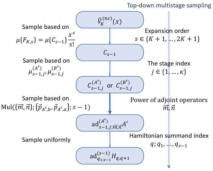
Now, we analyze the space and time cost of the whole sampling algorithm in Algorithm 2. The calculation of the 11-norms of CsC_{s} and its components Cs,j(A)C_{s,j}^{(A^{\prime})} and Cs,j(B)C_{s,j}^{(B^{\prime})} requires 𝒪(Kκ)\mathcal{O}(K\kappa) spacetime resources. Consider a parallel calculation, we need 𝒪(Kκ)\mathcal{O}(K\kappa) spatial resources and 𝒪(1)\mathcal{O}(1) time resources. We store all the above 11-norm coefficients in the memory with the size 𝒪(Kκ)\mathcal{O}(K\kappa). The sampling of FK,sF_{K,s} from KK discrete values requires 𝒪(logK)\mathcal{O}(\log{K}) steps Bringmann and Panagiotou (2012). For a given nested commutator Cs1C_{s-1}, the sampling of Cs,j(A)C_{s,j}^{(A^{\prime})} and Cs,j(B)C_{s,j}^{(B^{\prime})} from κ\kappa discrete values requires 𝒪(logκ)\mathcal{O}(\log{\kappa}) steps. The multinomial sampling of the power of adjoint operators m\vec{m} and n\vec{n} requires 𝒪(slogκ)\mathcal{O}(s\log{\kappa}) steps. Finally, the uniform sampling of the Hamiltonian summands from the light-cone region requires 𝒪(slogn)\mathcal{O}(s\log{n}) steps. To summarize, the space and time cost of Algorithm 2 are 𝒪(Kκ)\mathcal{O}(K\kappa) and 𝒪(K(logκ+logn))\mathcal{O}(K(\log{\kappa}+\log{n})), respectively.

Appendix E NESTED COMMUTATOR COMPENSATION FOR TROTTER FORMULAS OF GENERAL HAMILTONIANS

We now extend the methods to analyze the lattice model Hamiltonian to a general Hamiltonian. Consider a LL-sparse Hamiltonian with the form H=l=1LHlH=\sum_{l=1}^{L}H_{l}. The KKth-order Trotter formula (K=1K=1 or 2k2k, k+k\in\mathbb{N}_{+}) for U(x)=eixHU(x)=e^{-ixH} can be written as

SK(x)=j=1κl=1Leixa(j,l)Hπj(l).S_{K}(x)=\prod_{j=1}^{\kappa}\prod_{l=1}^{L}e^{-ixa_{(j,l)}H_{\pi_{j}(l)}}. (228)

Here, κ\kappa is the number of stages in the Trotter formula, that is, how many times each Hamiltonian component HlH_{l} is repeated in the implementation. We have κ=1\kappa=1 for K=1K=1 and κ=2×5k1\kappa=2\times 5^{k-1} when K=2kK=2k. The stage length coefficients a(j,l)a_{(j,l)} are determined based on Eq. 24 and Eq. 25. The permutation πj\pi_{j} indicates the ordering of the summands {Hl}\{H_{l}\} within the jjth stage in the Trotter formula. In Suzuki’s constructions Suzuki (1990) of Trotter formulas considered in this work, we alternately reverse the ordering of summands between neighboring stages.

In what follows, we omit the subscript KK in SK(x)S_{K}(x) for simplicity. To further simplify the notation, we introduce the lexicographical order Childs et al. (2021) for the pair of tuples (j,l)(j,l) in Eq. 228. For two pairs of tuples (j,l)(j,l) and (j,l)(j^{\prime},l^{\prime}), we have

  1. 1.

    (j,l)(j,l)(j,l)\succeq(j^{\prime},l^{\prime}) if j>jj>j^{\prime}, or if j=jj=j^{\prime} and l>ll>l^{\prime}.

  2. 2.

    (j,l)(j,l)(j,l)\succ(j^{\prime},l^{\prime}) if (j,l)(j,l)(j,l)\succeq(j^{\prime},l^{\prime}) and (j,l)(j,l)(j,l)\neq(j^{\prime},l^{\prime}).

We can also define (j,l)(j,l)(j,l)\preceq(j^{\prime},l^{\prime}) and (j,l)(j,l)(j,l)\prec(j^{\prime},l^{\prime}) in the same way. We denote the number of different tuples (j,l)(j,l) in SK(x)S_{K}(x) as Υ\Upsilon, which is usually equal to κL\kappa L. We can then express SK(x)S_{K}(x) and SK(x)S_{K}(x)^{\dagger} in the following way:

SK(x)=(j,l)eixa(j,l)Hπj(l),SK(x)=(j,l)eixa(j,l)Hπj(l).\displaystyle S_{K}(x)=\prod_{(j,l)}^{\leftarrow}e^{-ixa_{(j,l)}H_{\pi_{j}(l)}},\quad S_{K}(x)^{\dagger}=\prod_{(j,l)}^{\rightarrow}e^{ixa_{(j,l)}H_{\pi_{j}(l)}}. (229)

Similar to the case of lattice Hamiltonians, based on Eq. 94 and Eq. 111, we can expand the Trotter remainder VK(x)V_{K}(x) to the following form:

VK(x)=I+FL(x)+FK,𝓇𝓈(x),V_{K}(x)=I+F_{L}(x)+F_{K,\mathcal{res}}(x), (230)

where

FL(x)\displaystyle F_{L}(x) :=s=K2KCsxs+1(s+1)!,\displaystyle=\sum_{s=K}^{2K}C_{s}\frac{x^{s+1}}{(s+1)!}, (231)
FK,𝓇𝓈(x)\displaystyle F_{K,\mathcal{res}}(x) :=0x𝑑τ(MK(τ)JL(τ)+VK(τ)JK,res,2K(τ)).\displaystyle=\int_{0}^{x}d\tau\left(M_{K}(\tau)J_{L}(\tau)+V_{K}(\tau)J_{K,res,2K}(\tau)\right).

Here, FL(x)F_{L}(x) indicates the leading-order terms to be compensated by LCU formula, FK,𝓇𝓈(x)=𝒪(x2K+2)F_{K,\mathcal{res}}(x)=\mathcal{O}(x^{2K+2}) is the high-order part. In practice, we remove the high-order part with order s>2K+1s>2K+1 and implement only the leading-order terms

V~K(nc)(x)\displaystyle\tilde{V}_{K}^{(nc)}(x) =I+FL(x)=I+s=K+12K+1Cs1xss!\displaystyle=I+F_{L}(x)=I+\sum_{s=K+1}^{2K+1}C_{s-1}\frac{x^{s}}{s!} (232)
=1+(ηΣ(nc))2s=K+12K+1ηs(nc)ηΣ(nc)R2,s(nc)(ηΣ),\displaystyle=\sqrt{1+(\eta_{\Sigma}^{(nc)})^{2}}\sum_{s=K+1}^{2K+1}\frac{\eta_{s}^{(nc)}}{\eta_{\Sigma}^{(nc)}}R_{2,s}^{(nc)}(\eta_{\Sigma}),

where ηΣ(nc):=s=K+12K+1Cs11xss!\eta_{\Sigma}^{(nc)}:=\sum_{s=K+1}^{2K+1}\|C_{s-1}\|_{1}\frac{x^{s}}{s!}. The explicit form of R2,s(nc)(ηΣ)R_{2,s}^{(nc)}(\eta_{\Sigma}) can be obtained by the definitions in Eq. 109, Eq. 111 and the Pauli operator decomposition based on the nested-commutator form in Eq. 164.

We are going to finish the following tasks:

  1. 1.

    (App. E.1) Derive the explicit formulas for the leading-order expansion terms CsC_{s} with s=K,,2Ks=K,...,2K.

  2. 2.

    (App. E.2) Prove the 11-norm μK(nc)(x)\mu_{K}^{(nc)}(x) and error bound εK(nc)(x)\varepsilon_{K}^{(nc)}(x) of the LCU formula V~K(nc)(x)\tilde{V}^{(nc)}_{K}(x) in Eq. 232.

E.1 Derivation of nested-commutator form for general Hamiltonians

Based on the Trotter formulas in Eq. 229, we expand RK(x)R_{K}(x) in Eq. 92 as follows:

RK(x)\displaystyle R_{K}(x) =iγ=1Υγ=γ11eixaγHγ(aγHγ)\displaystyle=i\sum_{\gamma=1}^{\Upsilon}\prod_{\gamma^{\prime}=\gamma-1}^{1}e^{ixa_{\gamma^{\prime}}H_{\gamma^{\prime}}}\left(a_{\gamma}H_{\gamma}\right)\cdot (233)
γ=Υγ+1eixaγHγiHγ=Υ1eixaγHγ,\displaystyle\quad\prod_{\gamma^{\prime}=\Upsilon}^{\gamma+1}e^{ixa_{\gamma^{\prime}}H_{\gamma^{\prime}}}-iH\prod_{\gamma^{\prime}=\Upsilon}^{1}e^{ixa_{\gamma^{\prime}}H_{\gamma^{\prime}}},

JK(x)J_{K}(x) in Eq. 95 can then be written as,

JK(x)\displaystyle J_{K}(x) =iγ=1Υγ=γ+1ΥeixaγadHγ(aγHγ)\displaystyle=i\sum_{\gamma=1}^{\Upsilon}\prod_{\gamma^{\prime}=\gamma+1}^{\Upsilon}e^{-ixa_{\gamma^{\prime}}\mathrm{ad}_{H_{\gamma^{\prime}}}}(a_{\gamma}H_{\gamma}) (234)
iγ=1ΥeixaγadHγH.\displaystyle\quad-i\prod_{\gamma^{\prime}=1}^{\Upsilon}e^{-ixa_{\gamma^{\prime}}\mathrm{ad}_{H_{\gamma^{\prime}}}}H.

The derivative of JK(x)J_{K}(x) is

JK(s)(x)\displaystyle J^{(s)}_{K}(x) =iγ=1Υmγ+1mΥυ=γ+1Υmυ=s(smγ+1,,mΥ)(γ=γ+1Υ(iaγadHγ)mγeixaγadHγ)(aγHγ)\displaystyle=i\sum_{\gamma=1}^{\Upsilon}\sum_{\begin{subarray}{c}m_{\gamma+1}...m_{\Upsilon}\\ \sum_{\upsilon=\gamma+1}^{\Upsilon}m_{\upsilon}=s\end{subarray}}\binom{s}{m_{\gamma+1},...,m_{\Upsilon}}\left(\prod_{\gamma^{\prime}=\gamma+1}^{\Upsilon}(-ia_{\gamma^{\prime}}\mathrm{ad}_{H_{\gamma^{\prime}}})^{m_{\gamma^{\prime}}}e^{-ixa_{\gamma^{\prime}}\mathrm{ad}_{H_{\gamma^{\prime}}}}\right)(a_{\gamma}H_{\gamma}) (235)
im1mΥυ=1Υmυ=s(sm1,,mΥ)(γ=1Υ(iaγadHγ)mγeixaγadHγ)H.\displaystyle\quad-i\sum_{\begin{subarray}{c}m_{1}...m_{\Upsilon}\\ \sum_{\upsilon=1}^{\Upsilon}m_{\upsilon}=s\end{subarray}}\binom{s}{m_{1},...,m_{\Upsilon}}\left(\prod_{\gamma^{\prime}=1}^{\Upsilon}(-ia_{\gamma^{\prime}}\mathrm{ad}_{H_{\gamma^{\prime}}})^{m_{\gamma^{\prime}}}e^{-ixa_{\gamma^{\prime}}\mathrm{ad}_{H_{\gamma^{\prime}}}}\right)H.

Using the operator-valued Taylor-series expansion in Eq. 121, we have

Cs\displaystyle C_{s} =iγ=1Υ(j,l)m(j,l)=s(j,l)(j,l)(s{m(j,l)})((j,l)(j,l)(ia(j,l)adHπj(l))m(j,l))(a(j,l)Hπj(l))\displaystyle=i\sum_{\gamma=1}^{\Upsilon}\sum_{\begin{subarray}{c}\sum_{(j^{\prime},l^{\prime})}m_{(j^{\prime},l^{\prime})}=s\\ (j^{\prime},l^{\prime})\succ(j,l)\end{subarray}}\binom{s}{\{m_{(j^{\prime},l^{\prime})}\}}\left(\prod_{(j^{\prime},l^{\prime})\succ(j,l)}^{\leftarrow}(-ia_{(j^{\prime},l^{\prime})}\mathrm{ad}_{H_{\pi_{j^{\prime}}(l^{\prime})}})^{m_{(j^{\prime},l^{\prime})}}\right)(a_{(j,l)}H_{\pi_{j}(l)}) (236)
i(j,l)m(j,l)=s(s{m(j,l)})((j,l)(ia(j,l)adHπj(l))m(j,l))H\displaystyle\quad-i\sum_{\sum_{(j^{\prime},l^{\prime})}m_{(j^{\prime},l^{\prime})}=s}\binom{s}{\{m_{(j^{\prime},l^{\prime})}\}}\left(\prod_{(j^{\prime},l^{\prime})}^{\leftarrow}(-ia_{(j^{\prime},l^{\prime})}\mathrm{ad}_{H_{\pi_{j^{\prime}}(l^{\prime})}})^{m_{(j^{\prime},l^{\prime})}}\right)H

which is the nested-commutator form. Here, {m(j,l)}\{m_{(j^{\prime},l^{\prime})}\} are a group of integers whose summation is ss. Their corresponding multinomial coefficient is given by

(s{m(j,l)}):=s!(j,l)m(j,l)!.\binom{s}{\{m_{(j^{\prime},l^{\prime})}\}}:=\frac{s!}{\prod_{(j^{\prime},l^{\prime})}m_{(j^{\prime},l^{\prime})}!}. (237)

If we define

A(j,l)=Aγ=iaγHγ=ia(j,l)Hπj(l),A_{(j,l)}=A_{\gamma}=-ia_{\gamma}H_{\gamma}=-ia_{(j,l)}H_{\pi_{j}(l)}, (238)

we can simplify Eq. 236 as

Cs\displaystyle C_{s} =γ=1Υmγ+1mΥυ=γ+1Υmυ=s(smγ+1,,mΥ)γ=γ+1ΥadAγmγAγ\displaystyle=-\sum_{\gamma=1}^{\Upsilon}\sum_{\begin{subarray}{c}m_{\gamma+1}...m_{\Upsilon}\\ \sum_{\upsilon=\gamma+1}^{\Upsilon}m_{\upsilon}=s\end{subarray}}\binom{s}{m_{\gamma+1},...,m_{\Upsilon}}\prod_{\gamma^{\prime}=\gamma+1}^{\Upsilon}\mathrm{ad}_{A_{\gamma^{\prime}}}^{m_{\gamma^{\prime}}}A_{\gamma} (239)
+m1mΥυ=1Υmυ=s(sm1,,mΥ)γ=1ΥadAγmγ(iH),\displaystyle+\sum_{\begin{subarray}{c}m_{1}...m_{\Upsilon}\\ \sum_{\upsilon=1}^{\Upsilon}m_{\upsilon}=s\end{subarray}}\binom{s}{m_{1},...,m_{\Upsilon}}\prod_{\gamma^{\prime}=1}^{\Upsilon}\mathrm{ad}_{A_{\gamma^{\prime}}}^{m_{\gamma^{\prime}}}(-iH),

which is the summation of nested commutators. Therefore, one can still pair the leading-order terms FL(x)F_{L}(x) defined in Eq. 231 with II to suppress the 11-norm, shown in Eq. 232.

E.2 Norm bounds for the nested-commutator expansion

Now, we are going to bound the 11-norm μK(nc)(x)\mu^{(nc)}_{K}(x) and distance εK(nc)(x)\varepsilon^{(nc)}_{K}(x) of the truncated LCU formula V~K(nc)(x)\tilde{V}_{K}^{(nc)}(x) in Eq. 110 for a general Hamiltonian. We will use the following formula in the derivation.

Lemma 4 (Theorem 5 in Childs et al. (2021)).

Let A1,A2A_{1},A_{2}, …, ArA_{r} and BB be operators. Then, the conjugation has the expansion,

eτadAreτadA2eτadA1B\displaystyle e^{\tau\mathrm{ad}_{A_{r}}}.e^{\tau\mathrm{ad}_{A_{2}}}e^{\tau\mathrm{ad}_{A_{1}}}B (240)
=G0+G1τ++Gs1τs1(s1)!+Gres,s(τ).\displaystyle\quad=G_{0}+G_{1}\tau+.+G_{s-1}\frac{\tau^{s-1}}{(s-1)!}+G_{res,s}(\tau).

Here, G0,G1,,Gs1G_{0},G_{1},...,G_{s-1} are operators independent of τ\tau. The operator-valued function Gres,s(τ)G_{res,s}(\tau) is given by

Gres,s(τ):=γ=1rm1++mγ=smγ0eτadAreτadAγ+1\displaystyle G_{res,s}(\tau)=\sum_{\gamma=1}^{r}\sum_{\begin{subarray}{c}m_{1}+...+m_{\gamma}=s\\ m_{\gamma}\neq 0\end{subarray}}e^{\tau\mathrm{ad}_{A_{r}}}.e^{\tau\mathrm{ad}_{A_{\gamma+1}}}\cdot (241)
0τ𝑑τ2(ττ2)mγ1τm1++mγ1(mγ1)!mγ1!m1!eτ2adAγadAγmγadA1m1B.\displaystyle\int_{0}^{\tau}d\tau_{2}\frac{(\tau-\tau_{2})^{m_{\gamma}-1}\tau^{m_{1}+...+m_{\gamma-1}}}{(m_{\gamma}-1)!m_{\gamma-1}!...m_{1}!}e^{\tau_{2}\mathrm{ad}_{A_{\gamma}}}\mathrm{ad}_{A_{\gamma}}^{m_{\gamma}}.\mathrm{ad}_{A_{1}}^{m_{1}}B.

Furthermore, we have the spectral-norm bound,

Gres,s(τ)αcom(s)(Ar,,A1;B)|τ|ss!e2|τ|γ=1rAr,\|G_{res,s}(\tau)\|\leq\alpha_{\mathrm{com}}^{(s)}(A_{r},...,A_{1};B)\frac{|\tau|^{s}}{s!}e^{2|\tau|\sum_{\gamma=1}^{r}\|A_{r}\|}, (242)

for general operators and

Gres,s(τ)αcom(s)(Ar,,A1;B)|τ|ss!,\|G_{res,s}(\tau)\|\leq\alpha_{\mathrm{com}}^{(s)}(A_{r},...,A_{1};B)\frac{|\tau|^{s}}{s!}, (243)

when A1,,ArA_{1},...,A_{r} are anti-Hermitian. αcom(s)(Ar,,A1;B)\alpha_{\mathrm{com}}^{(s)}(A_{r},...,A_{1};B) is defined in Eq. 245.

We have the following proposition.

Proposition 13 (Trotter-LCU formula by nested-commutator compensation for general Hamiltonians).

For x>0x>0, V~K(x)\tilde{V}_{K}(x) in Eq. 232 is a (μ(nc)(x),ε(nc)(x))(\mu^{(nc)}(x),\varepsilon^{(nc)}(x))-LCU formula of KKth-order Trotter remainder VK(x)=U(x)SK(x)V_{K}(x)=U(x)S_{K}(x) with

μ(nc)\displaystyle\mu^{(nc)} 1+4κ2(s=K2KαH,1(s)xs+1(s+1)!)2,\displaystyle\leq\sqrt{1+4\kappa^{2}\left(\sum_{s=K}^{2K}\alpha_{H,1}^{(s)}\frac{x^{s+1}}{(s+1)!}\right)^{2}}, (244)
ε(nc)\displaystyle\varepsilon^{(nc)} 4κ2αH(K)s=K2KαH(s)xs+K+2s!(K+1)!(s+K+2)\displaystyle\leq 4\kappa^{2}\alpha_{H}^{(K)}\sum_{s=K}^{2K}\alpha_{H}^{(s)}\frac{x^{s+K+2}}{s!(K+1)!(s+K+2)}
+2κx2K+2(2K+2)!αH(2K+1).\displaystyle\quad+2\kappa\frac{x^{2K+2}}{(2K+2)!}\alpha^{(2K+1)}_{H}.

Here, we define the nested-commutator norms to be

αH(s):=l=1Lαcom(s)({Hπj(l)};Hl),\displaystyle\alpha^{(s)}_{H}=\sum_{l=1}^{L}\alpha_{\mathrm{com}}^{(s)}(\overleftarrow{\{H_{\pi_{j^{\prime}}(l^{\prime})}\}};H_{l}), (245)
αcom(s)(Ar,,A1;B):=\displaystyle\alpha_{\mathrm{com}}^{(s)}(A_{r},.,A_{1};B)=
m1++mr=s(sm1,,mr)adArmradA1m1B,\displaystyle\quad\sum_{m_{1}+...+m_{r}=s}\binom{s}{m_{1},...,m_{r}}\|\mathrm{ad}_{A_{r}}^{m_{r}}.\mathrm{ad}_{A_{1}}^{m_{1}}B\|,

where {Hπj(l)}\overleftarrow{\{H_{\pi_{j^{\prime}}(l^{\prime})}\}} indicates a sequence of Υ=κL\Upsilon=\kappa L summands with the lexicographical order given by the KKth-order Trotter formula in Eq. 229. αH,1(s)\alpha^{(s)}_{H,1} is defined similarly by replacing the spectral norm to 11-norm in Eq. 245.

Proof.

From Eq. 239 we can bound the 11-norm and spectral norm of CsC_{s} by

Cs\displaystyle\|C_{s}\| γ=1Υαcom(s)(AΥ,,Aγ+1;Aγ)\displaystyle\leq\sum_{\gamma=1}^{\Upsilon}\alpha_{\mathrm{com}}^{(s)}(A_{\Upsilon},.,A_{\gamma+1};A_{\gamma}) (246)
+αcom(s)(AΥ,,A1;H),\displaystyle\quad+\alpha_{\mathrm{com}}^{(s)}(A_{\Upsilon},.,A_{1};H),
Cs1\displaystyle\|C_{s}\|_{1} γ=1Υαcom,1(s)(AΥ,,Aγ+1;Aγ)\displaystyle\leq\sum_{\gamma=1}^{\Upsilon}\alpha_{com,1}^{(s)}(A_{\Upsilon},.,A_{\gamma+1};A_{\gamma})
+αcom,1(s)(AΥ,,A1;H).\displaystyle\quad+\alpha_{com,1}^{(s)}(A_{\Upsilon},.,A_{1};H).

Now, we are going to bound JK(x)\|J_{K}(x)\| and JK,res,2K(x)\|J_{K,res,2K}(x)\|. From Eq. 234 and using Lemma 4 we have

JK(x)\displaystyle J_{K}(x) =γ=1Υγ=γ+1ΥeadAγ(Aγ)+γ=1ΥeadAγ(iH)\displaystyle=-\sum_{\gamma=1}^{\Upsilon}\prod_{\gamma^{\prime}=\gamma+1}^{\Upsilon}e^{\mathrm{ad}_{A_{\gamma^{\prime}}}}(A_{\gamma})+\prod_{\gamma^{\prime}=1}^{\Upsilon}e^{\mathrm{ad}_{A_{\gamma^{\prime}}}}(-iH) (247)
=γ=1ΥGres,K(γ)(x)+Gres,K(0)(x).\displaystyle=\sum_{\gamma=1}^{\Upsilon}G^{(\gamma)}_{res,K}(x)+G^{(0)}_{res,K}(x).

In the second line, we use Lemma 4 to expand all the conjugate matrix exponentials to the following form:

γ=γ+1ΥeadAγ(Aγ)=G0(γ)+G1(γ)x+.\displaystyle\prod_{\gamma^{\prime}=\gamma+1}^{\Upsilon}e^{\mathrm{ad}_{A_{\gamma^{\prime}}}}(A_{\gamma})=G^{(\gamma)}_{0}+G^{(\gamma)}_{1}x+.. (248)
+GK1(γ)xK1(K1)!+Gres,K(γ),γ=1,2,Υ,\displaystyle\quad\quad+G^{(\gamma)}_{K-1}\frac{x^{K-1}}{(K-1)!}+G^{(\gamma)}_{res,K},\quad\gamma=1,2.,\Upsilon,
γ=1ΥeadAγ(iH)=G0(0)+G1(0)x+.\displaystyle\prod_{\gamma^{\prime}=1}^{\Upsilon}e^{\mathrm{ad}_{A_{\gamma^{\prime}}}}(-iH)=G^{(0)}_{0}+G^{(0)}_{1}x+..
+GK1(0)xK1(K1)!+Gres,K(0).\displaystyle\quad\quad+G^{(0)}_{K-1}\frac{x^{K-1}}{(K-1)!}+G^{(0)}_{res,K}.

The low-order terms Gs(γ)G_{s}^{(\gamma)} with s=0,1,,K1s=0,1,...,K-1 in Eq. 247 cancel out due to the order condition in Proposition 5. Therefore, we have

JK(x)γ=1ΥGres,K(γ)(x)+Gres,K(0)(x)\displaystyle\|J_{K}(x)\|\leq\sum_{\gamma=1}^{\Upsilon}\|G^{(\gamma)}_{res,K}(x)\|+\|G^{(0)}_{res,K}(x)\| (249)
xKK!(γ=1Υαcom(K)(AΥ,,Aγ+1;Aγ)+αcom(K)(AΥ,,A1;H))\displaystyle\leq\frac{x^{K}}{K!}\Big{(}\sum_{\gamma=1}^{\Upsilon}\alpha_{\mathrm{com}}^{(K)}(A_{\Upsilon},.,A_{\gamma+1};A_{\gamma})+\alpha_{\mathrm{com}}^{(K)}(A_{\Upsilon},.,A_{1};H)\Big{)}
2xKK!γ=1Υαcom(K)(AΥ,,A1;Hγ)\displaystyle\leq 2\frac{x^{K}}{K!}\sum_{\gamma=1}^{\Upsilon}\alpha_{\mathrm{com}}^{(K)}(A_{\Upsilon},.,A_{1};H_{\gamma})
=2κxKK!l=1Lαcom(K)({a(j,l)Hπj(l)};Hl)\displaystyle=2\kappa\frac{x^{K}}{K!}\sum_{l=1}^{L}\alpha_{\mathrm{com}}^{(K)}(\overleftarrow{\{a_{(j^{\prime},l^{\prime})}H_{\pi_{j^{\prime}}(l^{\prime})}\}};H_{l})
2κxKK!l=1Lαcom(K)({Hπj(l)};Hl)=:2κxKK!αH(K).\displaystyle\leq 2\kappa\frac{x^{K}}{K!}\sum_{l=1}^{L}\alpha_{\mathrm{com}}^{(K)}(\overleftarrow{\{H_{\pi_{j^{\prime}}(l^{\prime})}\}};H_{l})=:2\kappa\frac{x^{K}}{K!}\alpha^{(K)}_{H}.

Following the same way, we can bound Cs\|C_{s}\| and Cs1\|C_{s}\|_{1} in Eq. 246 as

Cs\displaystyle\|C_{s}\| 2καH(s),\displaystyle\leq 2\kappa\alpha^{(s)}_{H}, (250)
Cs1\displaystyle\|C_{s}\|_{1} 2καH,1(s).\displaystyle\leq 2\kappa\alpha^{(s)}_{H,1}.

Now, we are going to bound JK,res,2K(x)\|J_{K,res,2K}(x)\|. Similar to Eq. 247, we expand all the conjugate matrix exponentials to 2K2Kth-order,

JK(x)\displaystyle J_{K}(x) =γ=1Υγ=γ+1ΥeadAγ(Aγ)+γ=1ΥeadAγ(iH)\displaystyle=\sum_{\gamma=1}^{\Upsilon}\prod_{\gamma^{\prime}=\gamma+1}^{\Upsilon}e^{\mathrm{ad}_{A_{\gamma^{\prime}}}}(A_{\gamma})+\prod_{\gamma^{\prime}=1}^{\Upsilon}e^{\mathrm{ad}_{A_{\gamma^{\prime}}}}(-iH) (251)
=s=K2KCsxss!+γ=1ΥGres,2K+1(γ)(x)+Gres,2K+1(0)(x),\displaystyle=\sum_{s=K}^{2K}C_{s}\frac{x^{s}}{s!}+\sum_{\gamma=1}^{\Upsilon}G^{(\gamma)}_{res,2K+1}(x)+G^{(0)}_{res,2K+1}(x),

in the second line, we use the expansion of JK(x)J_{K}(x) in Eq. 104. Based on Eq. 249 we then have

JK,res,2K(x)=γ=1Υ\displaystyle J_{K,res,2K}(x)=\sum_{\gamma=1}^{\Upsilon} Gres,2K+1(γ)(x)+Gres,2K+1(0)(x)\displaystyle G^{(\gamma)}_{res,2K+1}(x)+G^{(0)}_{res,2K+1}(x) (252)
JK,res,2K(x)\displaystyle\Rightarrow\|J_{K,res,2K}(x)\| γ=1ΥGres,2K+1(γ)(x)+Gres,2K+1(0)(x)\displaystyle\leq\sum_{\gamma=1}^{\Upsilon}\|G^{(\gamma)}_{res,2K+1}(x)\|+\|G^{(0)}_{res,2K+1}(x)\|
2κx2K+1(2K+1)!αH(2K+1).\displaystyle\leq 2\kappa\frac{x^{2K+1}}{(2K+1)!}\alpha^{(2K+1)}_{H}.

We omit the derivation to the second line since it is the same as the one in Eq. 249.

Then we can bound MK(x)\|M_{K}(x)\| by

MK(x)0x𝑑τJK(τ)2κxK+1(K+1)!αH(K).\displaystyle\|M_{K}(x)\|\leq\int_{0}^{x}d\tau\|J_{K}(\tau)\|\leq 2\kappa\frac{x^{K+1}}{(K+1)!}\alpha_{H}^{(K)}. (253)

Finally, by applying Proposition 6 and using Eq. 250, we can bound the 11-norm μK(nc)(x)\mu^{(nc)}_{K}(x) as follows:

μK(nc)(x)1+4κ2(s=K2KαH,1(s)xs+1(s+1)!)2,\mu^{(nc)}_{K}(x)\leq\sqrt{1+4\kappa^{2}\left(\sum_{s=K}^{2K}\alpha_{H,1}^{(s)}\frac{x^{s+1}}{(s+1)!}\right)^{2}}, (254)

while the accuracy εK(nc)(x)\varepsilon^{(nc)}_{K}(x) can be bounded using Eq. 246, Eq. 252, and Eq. 253,

εK(nc)(x)=FK,𝓇𝓈(x)0x𝑑τ(MK(τ)JL(τ)+JK,res,2K(τ))\displaystyle\varepsilon^{(nc)}_{K}(x)=\|F_{K,\mathcal{res}}(x)\|\leq\int_{0}^{x}d\tau\left(\|M_{K}(\tau)\|\|J_{L}(\tau)\|+\|J_{K,res,2K}(\tau)\|\right) (255)
0x𝑑τ(4κ2τK+1(K+1)!αH(K)s=K2KαH(s)τss!+2κτ2K+1(2K+1)!αH(2K+1))\displaystyle\leq\int_{0}^{x}d\tau\left(4\kappa^{2}\frac{\tau^{K+1}}{(K+1)!}\alpha_{H}^{(K)}\sum_{s=K}^{2K}\alpha_{H}^{(s)}\frac{\tau^{s}}{s!}+2\kappa\frac{\tau^{2K+1}}{(2K+1)!}\alpha^{(2K+1)}_{H}\right)
4κ2αH(K)s=K2KαH(s)xs+K+2s!(K+1)!(s+K+2)+2κx2K+2(2K+2)!αH(2K+1).\displaystyle\leq 4\kappa^{2}\alpha_{H}^{(K)}\sum_{s=K}^{2K}\alpha_{H}^{(s)}\frac{x^{s+K+2}}{s!(K+1)!(s+K+2)}+2\kappa\frac{x^{2K+2}}{(2K+2)!}\alpha^{(2K+1)}_{H}.

From Proposition 13 we can see that, to characterize the performance of the Trotter-LCU algorithm, we only need to estimate the values of αH(s)\alpha^{(s)}_{H} and αH,1(s)\alpha^{(s)}_{H,1} for a given Hamiltonian. We can further simplify the form of αH(s)\alpha_{H}^{(s)} by the following upper bound Childs et al. (2021),

αH(s)\displaystyle\alpha_{H}^{(s)} κsls+1=1Ll2=1L[Hls+1,[Hl2,Hl]]]\displaystyle\leq\kappa^{s}\sum_{l_{s+1}=1}^{L}.\sum_{l_{2}=1}^{L}\|[H_{l_{s+1}},.[H_{l_{2}},H_{l}]].]\| (256)
=:κsα~com(H),\displaystyle=:\kappa^{s}\tilde{\alpha}_{\mathrm{com}}(H),

which is because the commutator terms in the left-hand side must be of the form on the right. Moreover, if we fix one term [Hls+1,[Hl2,Hl]]]\|[H_{l_{s+1}},...[H_{l_{2}},H_{l}]]...]\| on the right-hand side, we can find at most κs\kappa^{s} times of this term on the left-hand side.

Appendix F SOME USEFUL FORMULAS IN THE PROOF

Lemma 5 (Tail bound for the Poisson distribution (Theorem 1 in Canonne (2016))).

Suppose X^\hat{X} is a random variable with Poisson distribution so that Pr(X^=s)=Poi(s;x)=exxss!\Pr(\hat{X}=s)=\mathrm{Poi}(s;x)=e^{-x}\frac{x^{s}}{s!}, where x>0x>0 is the expectation value. Then, for any ϵ>0\epsilon>0, we have,

Pr(X^x+ϵ)eϵ22xh(ϵx),\Pr(\hat{X}\geq x+\epsilon)\leq e^{-\frac{\epsilon^{2}}{2x}h(\frac{\epsilon}{x})}, (257)

and, for any 0<ϵ<x0<\epsilon<x,

Pr(X^xϵ)eϵ22xh(ϵx).\Pr(\hat{X}\leq x-\epsilon)\leq e^{-\frac{\epsilon^{2}}{2x}h(-\frac{\epsilon}{x})}. (258)

Here, h(u):=2(1+u)ln(1+u)uu2h(u):=2\frac{(1+u)\ln(1+u)-u}{u^{2}} for u1u\geq-1.

From Lemma 5 we have the following corollaries.

Corollary 1.

For x>0x>0 and positive integer kk such that x<k+1x<k+1, we have

s=k+1xss!(exk+1)k+1.\sum_{s=k+1}^{\infty}\frac{x^{s}}{s!}\leq\left(\frac{ex}{k+1}\right)^{k+1}. (259)
Proof.

We set ϵ=(k+1)x\epsilon=(k+1)-x. From Lemma 5 we have

Pr(X^k+1)\displaystyle\Pr(\hat{X}\geq k+1) exp((k+1x)22xh(k+1xx))\displaystyle\leq\exp\left(-\frac{(k+1-x)^{2}}{2x}h(\frac{k+1-x}{x})\right) (260)
=ex(exk+1)k+1.\displaystyle=e^{-x}\left(\frac{ex}{k+1}\right)^{k+1}.

Therefore,

Pr(X^k+1)=exs=k+1xss!ex(exk+1)k+1\displaystyle\quad\Pr(\hat{X}\geq k+1)=e^{-x}\sum_{s=k+1}^{\infty}\frac{x^{s}}{s!}\leq e^{-x}\left(\frac{ex}{k+1}\right)^{k+1} (261)
s=k+1xss!(exk+1)k+1.\displaystyle\Rightarrow\sum_{s=k+1}^{\infty}\frac{x^{s}}{s!}\leq\left(\frac{ex}{k+1}\right)^{k+1}.

Corollary 2.

For x>0x>0 and positive integer kk such that x<k+1x<k+1, we have

exs=1kxss!eexk+1.e^{x}-\sum_{s=1}^{k}\frac{x^{s}}{s!}\leq e^{ex^{k+1}}. (262)
Proof.

When x<k+1x<k+1, from Corollary 1 we have

exs=k+1xss!ex(exk+1)k+1\displaystyle\quad e^{-x}\sum_{s=k+1}^{\infty}\frac{x^{s}}{s!}\leq e^{-x}\left(\frac{ex}{k+1}\right)^{k+1} (263)
1exexs=1kxss!ex(exk+1)k+1\displaystyle\Rightarrow 1-e^{-x}-e^{-x}\sum_{s=1}^{k}\frac{x^{s}}{s!}\leq e^{-x}\left(\frac{ex}{k+1}\right)^{k+1}
exs=1kxss!1+(exk+1)k+1\displaystyle\Rightarrow e^{x}-\sum_{s=1}^{k}\frac{x^{s}}{s!}\leq 1+\left(\frac{ex}{k+1}\right)^{k+1}
1+(ex)k+1(k+1)!eexk+1.\displaystyle\quad\leq 1+\frac{(ex)^{k+1}}{(k+1)!}\leq e^{ex^{k+1}}.

Lemma 6 (Proposition 9 in Wan et al. (2022)).

For any β>0\beta>0, 1>ϵ>01>\epsilon>0, we have (eβs)sϵ\left(\frac{e\beta}{s}\right)^{s}\leq\epsilon, for all sf(β,ϵ):=ln(1ϵ)W0(1eβln(1ϵ))s\geq f(\beta,\epsilon):=\frac{\ln(\frac{1}{\epsilon})}{W_{0}\left(\frac{1}{e\beta}\ln(\frac{1}{\epsilon})\right)}. Here, W0(y)W_{0}(y) is the principle branch of the Lambert WW function.

Lemma 7 (Theorem 2.7 in Hoorfar and Hassani (2008)).

When yey\geq e we have

ln(y)lnln(y)+12lnln(y)ln(y)W0(y)\displaystyle\ln(y)-\ln\ln(y)+\frac{1}{2}\frac{\ln\ln(y)}{\ln(y)}\leq W_{0}(y) (264)
ln(y)lnln(y)+ee1lnln(y)ln(y).\displaystyle\quad\leq\ln(y)-\ln\ln(y)+\frac{e}{e-1}\frac{\ln\ln(y)}{\ln(y)}.

Appendix G ADDITIONAL NUMERICAL RESULTS

In this section, we provide more numerical results by comparing the gate costs of Trotter-LCU algorithms with other typical algorithms, especially the Trotter algorithm and “post-Trotter” algorithm with best performance, i.e., the fourth-order Trotter algorithm and the quantum signal processing (QSP) algorithm. We will mainly consider two different scenarios—generic LL-sparse Hamiltonians and lattice Hamiltonians. In the former case, the previously known best result is given by the QSP algorithm Low and Chuang (2017); in the latter case, since we can take advantage of the spacial locality and commutator information, the fourth-order Trotter algorithm is known to have the best performance Childs et al. (2018); Childs and Su (2019).

For the Trotter algorithms and Trotter-LCU algorithms, we first compile the circuit to 𝒞𝒩𝒪𝒯\mathcal{CNOT} gates, single-qubit Clifford gates and non-Clifford ZZ-axis rotation gate Rz(θ)=eiθZR_{z}(\theta)=e^{i\theta Z}. On the other hand, the circuit compilation for the QSP algorithm is more complicated: we need to decompose the state-preparation oracles and the select-HH gates. We follow the qROM design in Ref. Babbush et al. (2018b) based on a sawtooth structure. The detailed gate resource analysis can be found in a companion work Sun et al. (2024). Based on the qROM design, we decompose all the state preparation oracles and the select-HH gates to Toffoli gates, which can be further decomposed to 𝒞𝒩𝒪𝒯\mathcal{CNOT} gates, single-qubit Clifford gates and TT gates.

For a fair comparison between the gate costs of Trotter, Trotter-LCU and QSP algorithms, we need to further compile the ZZ-axis rotation gate Rz(θ)R_{z}(\theta) to TT gate. We follow the gate compilation work in Ref. Bocharov et al. (2015), where the expected TT-gate number to compile Rz(θ)R_{z}(\theta) with random θ\theta is about

cT=1.149log2(1/ϵ)+9.2,c_{T}=1.149\log_{2}(1/\epsilon)+9.2, (265)

where ϵ\epsilon is the compilation accuracy. We set the accuracy ϵ=1015\epsilon=10^{-15} in the later resource estimation. In this case, cT66c_{T}\approx 66.

G.1 Generic LL-sparse Hamiltonians

For the generic LL-sparse Hamiltonian, we choose the 22-local Hamiltonian

H=i,jJijXiXj+iZi,H=\sum_{i,j}J_{ij}X_{i}X_{j}+\sum_{i}Z_{i}, (266)

with Jij=1J_{ij}=1 as an example, in which case we ignore the commutator information between different Hamiltonian summands. This simple model works as a representative of many generic Hamiltonians where the commutator information is not helpful or too complicated to count on, e.g., quantum chemistry Hamiltonian for the molecules. Without the commutator information, the former best Hamiltonian simulation algorithm is QSP Low and Chuang (2017).

In Fig. 13 and Fig. 14, we estimate and compare the 𝒞𝒩𝒪𝒯\mathcal{CNOT} and TT gate counts for the PTSC algorithms, QSP and fourth-order Trotter algorithm with respect to the evolution time. We choose fourth-order Trotter algorithm with random permutation since it performs the best over all the Trotter algorithms. The gate counting method for fourth-order Trotter with random permutation is based on the analytical bounds in Ref. Childs et al. (2019). For the QSP algorithm, we estimate the gate count based on the QROM construction in Ref. Babbush et al. (2018b). Only the high-accuracy results ε=105\varepsilon=10^{-5} for our method and quantum signal processing are presented since our method and quantum signal processing has a logarithmic dependence and hence are less prone to the accuracy while the Trotter formulae has polynomial dependence on the accuracy.

Refer to caption
Figure 13: CNOT-gate number estimation for simulating the generic LL-sparse Hamiltonian with an increasing time. The system size is set as n=20n=20. The simulation is exemplified with the 22-local Hamiltonian in Eq. 266.
Refer to caption
Figure 14: TT-gate number estimation for simulating the generic LL-sparse Hamiltonian with an increasing time. The system size is set as n=20n=20. The simulation is exemplified with the 22-local Hamiltonian in Eq. 266.

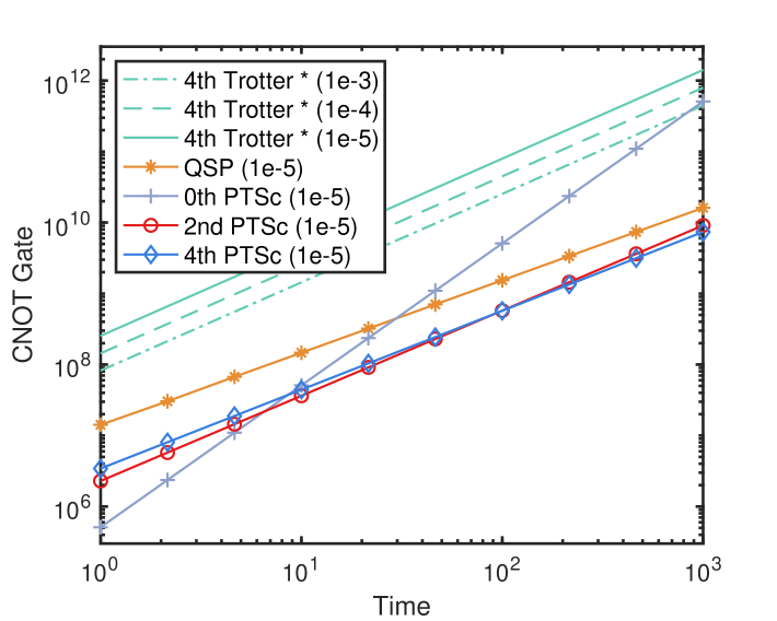
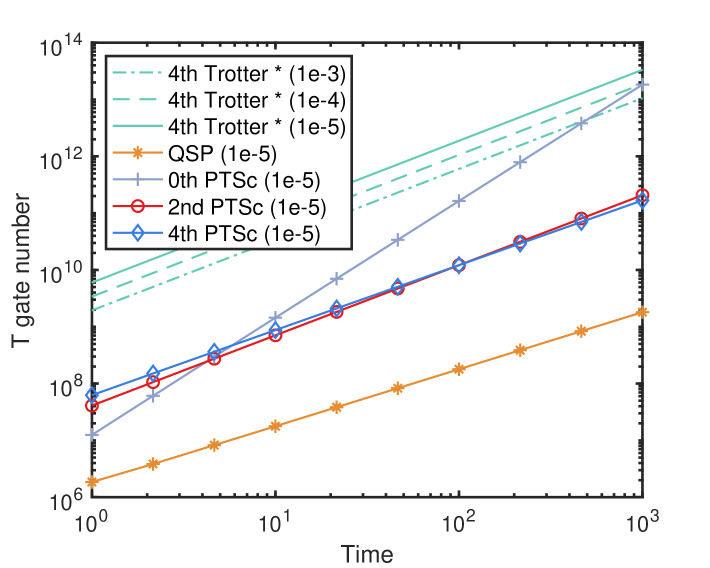
From Fig. 13 and Fig. 14 we can see that, the PTSC algorithm owns a lower 𝒞𝒩𝒪𝒯\mathcal{CNOT} gate cost than the QSP algorithm because it does not need the qROM for classical data loading. On the other hand, the PTSC algorithms have a larger T-gate cost than QSP algorithm. This is mainly due to the compilation cost of arbitrary ZZ-axis rotation gate Rz(θ)R_{z}(\theta) to TT gates: for each Rz(θ)R_{z}(\theta) gate with a random phase θ\theta, we need cT=66c_{T}=66 TT gates on average to compile it to the accuracy of ε=1015\varepsilon=10^{-15}. In the Trotter or Trotter-LCU algorithms, the non-Clifford gate cost mainly originates from the Rz(θ)R_{z}(\theta) gates: in each segment, there are roughly κKL\kappa_{K}L Rz(θ)R_{z}(\theta) gates, leading to about κKcTL\kappa_{K}c_{T}L compiled TT gates. As a comparison, there are only few Rz(θ)R_{z}(\theta) gates in QSP algorithm used for the phase iteraction procedure to realize the Jacobi-Anger polynomials. The major non-Clifford gate cost lies in the compilation of state-preparation oracles and the select-HH gates, each of which can be realized by about 4L4L TT gates based on the qROM design in Ref. Babbush et al. (2018b).

In Fig. 15 we compare the qubit number required to implement the QSP and the PTSC algorithms, based on the 22-local Hamiltonian model. We can see a clear advantage of the spacial resource cost of PTSC to QSP algorithm.

Refer to caption
Figure 15: Qubit number required for simulating the generic LL-sparse Hamiltonian with an increasing system size. The simulation is exemplified with the 22-local Hamiltonian in Eq. 266.

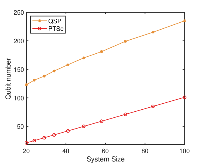
G.2 Lattice Hamiltonians

Now, we consider the case of lattice Hamiltonians. We consider the Heisenberg model, H=Jiσiσi+1+hiZiH=J\sum_{i}\vec{\sigma}_{i}\vec{\sigma}_{i+1}+h\sum_{i}Z_{i}, where σi:=(Xi,Yi,Zi)\vec{\sigma}_{i}:=(X_{i},Y_{i},Z_{i}) is the vector of Pauli operators on the iith qubit and J=h=1J=h=1.

We compare the 𝒞𝒩𝒪𝒯\mathcal{CNOT} and TT gate number of the second-order NCC algorithm, QSP and fourth-order Trotter algorithm in Fig. 16 and Fig. 17, respectively. The fourth-order Trotter error analysis is based on the nested-commutator bound (Proposition M.1 in Ref. Childs et al. (2021)), which is currently the tightest Trotter error bound. The performance of our second-order NCC algorithm is analyzed based on the detailed analysis in Section B. We explicitly calculate the 11-norm of the LCU formula and use the analytical bound for the accuracy analysis. Here, we do not introduce the empirical analysis for a fair comparison. Since the explicit evaluation of our fourth-order NCC algorithm is complicated, we mainly present the results for our second-order algorithm.

As addressed in Childs et al. (2021); Childs and Su (2019), fourth-order Trotter formula shows a near-optimal scaling with respect to the system size for the lattice model, which is clearly shown in Fig. 16. From Fig. 16 we can see that, our second-order NCC algorithm shows an advantage over the fourth-order Trotter algorithm. Furthermore, the nn and tt scaling of our second-order NCC algorithm is similar to the fourth-order Trotter algorithm, which is near optimal.

Refer to caption
Figure 16: CNOT gate-number estimation for simulating the Heisenberg Hamiltonian using the nested-commutator bound with an increasing system size nn. The simulation time is set as t=nt=n. The fourth-order Trotter formula uses the nested-commutator bound shown in Proposition M.1 in Childs et al. (2021). Our result is based on second-order NCC algorithm with the analysis in Section B.
Refer to caption
Figure 17: TT gate-number estimation for simulating the Heisenberg Hamiltonian using the nested-commutator bound with an increasing system size nn. The stage is set up the same as that in Fig. 16.

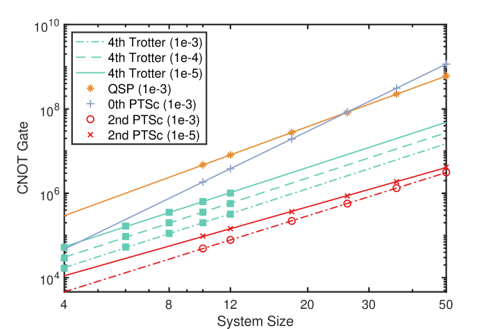
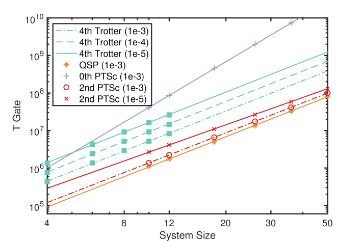
Appendix H COHERENT IMPLEMENTATION

In the main text, we primarily focus on the random-sampling implementation of the Trotter-LCU algorithms due to its simplicity. When the block encoding of an LCU formula of VV is feasible on a fault-tolerant quantum computer, we can also consider the coherent implementation of the Trotter-LCU algorithms.

The gate complexity of the coherent implementation of the Trotter-LCU algorithm is determined by the segment number ν\nu, the Trotter order KK, the number of elementary unitaries Γ\Gamma and the gate complexity of each elementary unitary in the LCU formula. The value Γ\Gamma is related to the specific compensation method we use, which is usually proportional to LL and the truncation order scs_{c}. The gate complexity is

NK=𝒪(ν(κKL+Γ)),\displaystyle N_{K}=\mathcal{O}(\nu(\kappa_{K}L+\Gamma)), (267)

To estimate the segment number ν\nu, we first find a proper evolution time xx such that the 11-norm μx2\mu_{x}\leq 2. The segment number is then ν=t/x\nu=t/x.

For the PTSC formula, based on the 11-norm bound in Theorem 1, we find that to ensure μx2\mu_{x}\leq 2, it is sufficient to set x=12λ(ln2e+ck)12K+2=𝒪(1λ)x=\frac{1}{2\lambda}(\frac{\ln 2}{e+c_{k}})^{\frac{1}{2K+2}}=\mathcal{O}(\frac{1}{\lambda}). As a result, the number of segment ν=t/x=𝒪(λt)\nu=t/x=\mathcal{O}(\lambda t). From Eq. 267, the overall gate complexity of the algorithm is

NK(p)=𝒪(ν(κKL+Γ))=𝒪(λtLlog(1/ε)loglog(1/ε)),N_{K}^{(p)}=\mathcal{O}(\nu(\kappa_{K}L+\Gamma))=\mathcal{O}\left(\lambda tL\frac{\log(1/\varepsilon)}{\log\log(1/\varepsilon)}\right), (268)

which is the same as the case when no Trotter formula is applied Berry et al. (2015).

For the NCC formula, based on the 11-norm bound in Theorem 2, we find that to ensure μx2\mu_{x}\leq 2, we need to set x=1βΛ1(2ln2(K!)2(nκ)2)12K+2ν=𝒪(n1K+1t)x=\frac{1}{\beta\Lambda_{1}}\left(\frac{2\ln 2(K!)^{2}}{(n\kappa)^{2}}\right)^{\frac{1}{2K+2}}\Rightarrow\nu=\mathcal{O}(n^{\frac{1}{K+1}}t). To achieve an overall simulation accuracy ε\varepsilon, we need

νεK(nc)(x)εν=𝒪(n22K+1t1+12K+1ε12K+1).\nu\varepsilon_{K}^{(nc)}(x)\leq\varepsilon\Rightarrow\nu=\mathcal{O}(n^{\frac{2}{2K+1}}t^{1+\frac{1}{2K+1}}\varepsilon^{-\frac{1}{2K+1}}). (269)

Therefore, it suffice to choose ν\nu to be

ν=𝒪(n22K+1t1+12K+1ε12K+1).\nu=\mathcal{O}(n^{\frac{2}{2K+1}}t^{1+\frac{1}{2K+1}}\varepsilon^{-\frac{1}{2K+1}}). (270)

In each segment, we need to implement KKth-order Trotter formula and the (K+1)(K+1)th- to (2K+1)(2K+1)th-order LCU formula. The number of elementary unitaries is 𝒪(n)\mathcal{O}(n). Therefore, the overall gate complexity is

NK(nc)=𝒪(n1+22K+1t1+12K+1ε12K+1).N_{K}^{(nc)}=\mathcal{O}(n^{1+\frac{2}{2K+1}}t^{1+\frac{1}{2K+1}}\varepsilon^{-\frac{1}{2K+1}}). (271)

Although it does not achieve the logarithmic accuracy dependence seen in standard post-Trotter algorithms Berry et al. (2015); Low and Chuang (2019), it has the unique advantage of a system-size dependence of 𝒪(n)\mathcal{O}(n), which could be advantageous in large-scale coherent Hamiltonian simulations.

References