Simplification Methods for Sum-of-Squares Programs

A polynomial is a sum-of-squares (SOS) if it can be expressed as a sum of squares of other polynomials. There are close connections between SOS polynomials and positive semidefinite matrices [3, 2, 4, 13, 11, 7, 12]. For a given polynomial the search for an SOS decomposition is equivalent to a linear matrix inequality feasibility problem. It is also possible to formulate optimization problems with polynomial sum-of-squares constraints [11, 12]. There is freely available software that can be used to solve these SOS feasibility and optimization problems [14, 8, 1, 6]. Many nonlinear analysis problems, e.g. Lyapunov stability analysis, can be formulated within this optimization framework [11, 12, 19, 20].

Computational growth is a significant issue for these optimization problems. For example, consider the search for an SOS decomposition: given a polynomial $p$ and a vector of monomials $z$, does there exist a matrix $Q\succeq 0$ such that $p=z^{T}Qz$? The computation required to solve the corresponding linear matrix inequality feasibility problem grows with the number of monomials in the vector $z$. The Newton polytope [15, 18] is a method to prune unnecessary monomials from the vector $z$. This method is implemented in SOSTOOLs [14]. One drawback is that this method requires the construction of a convex hull and this construction itself can be time consuming for polynomials with many terms.

This paper presents an alternative monomial reduction method called the zero diagonal algorithm. This algorithm is based on a simple property of positive semidefinite matrices: if the $(i,i)$ diagonal entry of a positive semidefinite matrix is zero then the entire $i^{th}$ row and column must be zero. The zero diagonal algorithm simply searches for diagonal entries of $Q$ that are constrained to be zero and then prunes the corresponding monomials. This algorithm can be implemented with very little computational cost using the Matlab find command. It is shown that final list of monomials returned by the zero diagonal algorithm is never larger than the pruned list obtained from the Newton polytope method. For some problems the zero diagonal algorithm returns a strictly smaller set of monomials. Results contained in this paper are similar to and preceded by those found in the prior work [9, 21].

The basic idea in the zero diagonal algorithm is then extended to a more general simplification method for sum-of-squares programs. The more general method also removes free variables that are implicitly constrained to be equal to zero. This can improve the numerical conditioning and reduce the computation time required to solve the SOS program. Both the zero diagonal elimination algorithm and the simplification procedure for SOS programs are implemented in SOSOPT [1].

$\mathbb{N}$ denotes the set of nonnegative integers, $\{0,1,\ldots\}$, and $\mathbb{N}^{n}$ is the set of $n$-dimensional vectors with entries in $\mathbb{N}$. For $\alpha\in\mathbb{N}^{n}$, a monomial in variables $\{x_{1},\ldots,x_{n}\}$ is given by $x^{\alpha}:=x_{1}^{\alpha_{1}}x_{2}^{\alpha_{2}}\cdots x_{n}^{\alpha_{n}}$. $\alpha$ is the degree vector associated with the monomial $x^{\alpha}$. The degree of a monomial is defined as $\deg{x^{\alpha}}:=\sum_{i=1}^{n}\alpha_{i}$. A polynomial is a finite linear combination of monomials:

$\displaystyle p:=\sum_{\alpha\in{\cal A}}c_{\alpha}x^{\alpha}=\sum_{\alpha\in{\cal A}}c_{\alpha}x_{1}^{\alpha_{1}}x_{2}^{\alpha_{2}}\cdots x_{n}^{\alpha_{n}}$

(1)

where $c_{\alpha}\in\mathbb{R}$, $c_{\alpha}\neq 0$, and ${\cal A}$ is a finite collection of vectors in $\mathbb{N}^{n}$. $\mathbb{R}[x]$ denotes the set of all polynomials in variables $\{x_{1},\ldots,x_{n}\}$ with real coefficients. Using the definition of $\deg$ for a monomial, the degree of $p$ is defined as $\deg{p}:=\max_{\alpha\in{\cal A}}\ \ [\deg{x^{\alpha}}]$.

A polynomial $p$ is a sum-of-squares (SOS) if there exist polynomials $\{f_{i}\}_{i=1}^{m}$ such that $p=\sum_{i=1}^{m}f_{i}^{2}$. The set of SOS polynomials is a subset of $\mathbb{R}[x]$ and is denoted by ${\Sigma[x]}$. If $p$ is a sum-of-squares then $p(x)\geq 0$ $\forall x\in\mathbb{R}^{n}$. However, non-negative polynomials are not necessarily SOS [16].

Define $z$ as the column vector of all monomials in variables $\{x_{1},\ldots,x_{n}\}$ of degree $\leq d$: ¹¹1Any ordering of the monomials can be used to form $z$. In Equation 2, $x^{\alpha}$ precedes $x^{\beta}$ in the definition of $z$ if $\deg{x^{\alpha}}<\deg{x^{\beta}}$ OR $\deg{x^{\alpha}}=\deg{x^{\beta}}$ and the first nonzero entry of $\alpha-\beta\mbox{ is }>0$.

$\displaystyle z:=\begin{bmatrix}1,\ x_{1},\ x_{2},\ \ldots,\ x_{n},\ x_{1}^{2},\ x_{1}x_{2},\ \ldots,\ x_{n}^{2},\ \ldots,\ x_{n}^{d}\end{bmatrix}^{T}$

(2)

There are $\left(\begin{smallmatrix}k+n-1\\ k\end{smallmatrix}\right)$ monomials in $n$ variables of degree $k$. Thus $z$ is a column vector of length $l_{z}:=\sum_{k=0}^{d}\left(\begin{smallmatrix}k+n-1\\ k\end{smallmatrix}\right)=\left(\begin{smallmatrix}n+d\\ d\end{smallmatrix}\right)$. If $f$ is a polynomial in $n$ variables with degree $\leq d$ then by definition $f$ is a finite linear combination of monomials of degree $\leq d$. Consequently, there exists $a\in\mathbb{R}^{l_{z}}$ such that $f=a^{T}z$.

Two useful facts from [15] are:

1. 1.

   If $p$ is a sum-of-squares then $p$ must have even degree.

2. 2.

   If $p$ is degree $2d$ ($d\in\mathbb{N}$) and $p=\sum_{i=1}^{m}f_{i}^{2}$ then $\deg{f_{i}}\leq d$ $\forall i$.

The following theorem, introduced as the “Gram Matrix” method by [4, 13], connects SOS polynomials and positive semidefinite matrices.

Determining if an SOS decomposition exists for a given polynomial $p$ is equivalent to a feasibility problem:

$\displaystyle\mbox{Find }Q\succeq 0\mbox{ such that }p=z^{T}Qz$

(3)

$Q$ is constrained to be positive semi-definite and equating coefficients of $p$ and $z^{T}Qz$ imposes linear equality constraints on the entries of $Q$. Thus this is a linear matrix inequality (LMI) feasibility problem. There is software available to solve for SOS decompositions [14, 8, 1]. These toolboxes convert the SOS feasibility problem to an LMI problem. The LMI problem is then solved with a freely available LMI solver, e.g. Sedumi [17], and an SOS decomposition is constructed if a feasible solution is found. These software packages also solve SOS synthesis problems where some of the coefficients of the polynomial are treated as free variables to be computed as part of the optimization. These more general SOS optimization problems are discussed further in Section V. Many analysis problems for polynomial dynamical systems can be posed within this SOS synthesis framework [11, 12, 19, 20].

As discussed in the previous section, the search for an SOS decomposition is equivalent to an LMI feasibility problem. One issue is that the computational complexity of this LMI feasibility problem grows with the dimension of the Gram matrix. For a polynomial of degree $2d$ in $n$ variables there are, in general, $l_{z}=\left(\begin{smallmatrix}n+d\\ d\end{smallmatrix}\right)$ monomials in $z$ and the Gram matrix $Q$ is $l_{z}\times l_{z}$. $l_{z}$ grows rapidly with both the number of variables and the degree of the polynomial. However, any particular polynomial $p$ may have an SOS decomposition with fewer monomials. The Newton Polytope [15, 18] is an algorithm to reduce the dimension $l_{z}$ by pruning unnecessary monomials from $z$.

First, some terminology is provided regarding polytopes [10, 5]. For any set ${\cal A}\subseteq\mathbb{R}^{n}$, $\mbox{convhull}(A)$ denotes the convex hull of ${\cal A}$. Let $C\subseteq\mathbb{R}^{n}$ be a convex set. A point $\alpha\in C$ is an extreme point if it does not belong to the relative interior of any segment $[\alpha_{1},\alpha_{2}]\subset C$. In other words, if $\exists\alpha_{1},\alpha_{2}\in C$ and $0<\lambda<1$ such that $\alpha=\lambda\alpha_{1}+(1-\lambda)\alpha_{2}$ then $\alpha_{1}=\alpha_{2}=\alpha$. A convex polytope (or simply polytope) is the convex hull of a non-empty, finite set $\{\alpha_{1},\ldots,\alpha_{p}\}\subseteq\mathbb{R}^{n}$. The extreme points of a polytope are called the vertices. Let $C$ be a polytope and let ${\cal V}$ be the (finite) set of vertices of $C$. Then $C=\mbox{convhull}({\cal V})$ and ${\cal V}$ is a minimal vertex representation of $C$. The polytope $C$ may be equivalently described as an intersection of a finite collection of halfspaces, i.e. there exists a matrix $H\in\mathbb{R}^{N\times n}$ and a vector $g\in\mathbb{R}^{N}$ such that $C=\{\alpha\in\mathbb{R}^{n}\ :\ H\alpha\leq g\}$. This is a facet or half-space representation of $C$.

The Newton Polytope (or cage) of a polynomial $p=\sum_{\alpha\in{\cal A}}c_{\alpha}x^{\alpha}$ is defined as $C(p):=\mbox{convhull}({\cal A})\subseteq\mathbb{R}^{n}$ [15]. The reduced Newton polytope is $\frac{1}{2}C(p):=\{\frac{1}{2}\alpha\ :\ \alpha\in C(p)\}$. The following theorem from [15] is a key result for monomial reduction. ²²2 A polynomial $p$ is a form if all monomials have the same degree. The results in [15] are stated and proved for forms. A given polynomial can be converted to a form by adding a single dummy variable of appropriate degree to each monomial. The results in [15] apply to polynomials by this homogenization procedure.

This theorem implies that any monomial $x^{\alpha}$ appearing in the vector $z$ of an SOS decomposition $z^{T}Qz$ must satisfy $\alpha\in\frac{1}{2}C(p)\cap\mathbb{N}^{n}$. This forms the basis for the Newton polytope method for pruning monomials: Let $p$ be a given polynomial of degree $2d$ in $n$ variables with monomial degree vectors specified by the finite set ${\cal A}$. First, create the $l_{z}\times 1$ vector $z$ consisting of all monomials of degree $\leq d$ in $n$ variables. There are $l_{z}=\left(\begin{smallmatrix}n+d\\ d\end{smallmatrix}\right)$ monomials in this complete list. Second, compute a half-space representation $\{\alpha\in\mathbb{R}^{n}\ :\ H\alpha\leq g\}$ for the reduced Newton polytope $\frac{1}{2}C(p)$. Third, prune out any monomials in $z$ that are not elements of $\frac{1}{2}C(p)$. This algorithm is implemented in SOSTOOLs [14]. The third step amounts to checking each monomial in $z$ to see if the corresponding degree vector satisfies the half-plane constraints $H\alpha\leq g$. This step is computationally very fast. The second step requires computing a half-plane representation for the convex hull of $\frac{1}{2}{\cal A}$. This can be done in Matlab, e.g. with convhulln. However, this step can be time-consuming when the polynomial has many terms (${\cal A}$ has many elements). The next section provides an alternative implementation of the Newton Polytope algorithm that avoids constructing the half-space representation of the reduced Newton polytope.

Example: Consider the following polynomial

$\displaystyle p=3x_{1}^{4}-2x_{1}^{2}x_{2}+7x_{1}^{2}-4x_{1}x_{2}+4x_{2}^{2}+1$

(4)

$p$ is a degree four polynomial in two variables. The list of all monomials in two variables with degree $\leq 2$ is:

$\displaystyle z=\begin{bmatrix}1&x_{1}&x_{2}&x_{1}^{2}&x_{1}x_{2}&x_{2}^{2}\end{bmatrix}^{T}$

(5)

The length of $z$ is $l_{z}=6$. An SOS decomposition of a degree four polynomial would, in general, include all six of these monomials. The Newton Polytope can be used to prune some unnecessary monomials in this list.

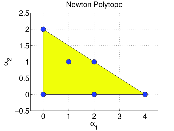
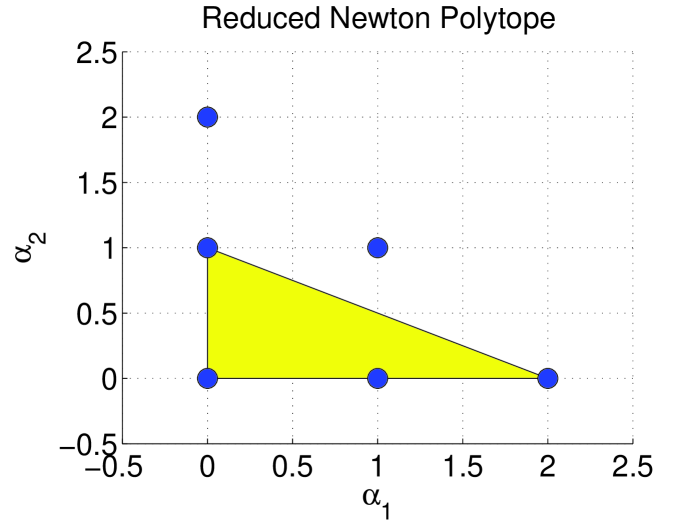
The set of monomial degree vectors for $p$ is ${\cal A}:=\{\left[\begin{smallmatrix}4\\ 0\end{smallmatrix}\right],\ \left[\begin{smallmatrix}2\\ 1\end{smallmatrix}\right],\ \left[\begin{smallmatrix}2\\ 0\end{smallmatrix}\right],\ \left[\begin{smallmatrix}1\\ 1\end{smallmatrix}\right],\ \left[\begin{smallmatrix}0\\ 2\end{smallmatrix}\right],\ \left[\begin{smallmatrix}0\\ 0\end{smallmatrix}\right]\}$. These vectors are shown as circles in Figure 1. The Newton Polytope $C(p)$ is the large triangle with vertices $\{\left[\begin{smallmatrix}4\\ 0\end{smallmatrix}\right],\ \left[\begin{smallmatrix}0\\ 0\end{smallmatrix}\right],\ \left[\begin{smallmatrix}0\\ 2\end{smallmatrix}\right]\}$. Figure 2 shows the degree vectors for the six monomials in $z$ (circles) and the reduced Newton polytope (large triangle). The reduced Newton polytope $\frac{1}{2}C(f)$ is the triangle with vertices $\{\left[\begin{smallmatrix}2\\ 0\end{smallmatrix}\right],\ \left[\begin{smallmatrix}0\\ 0\end{smallmatrix}\right],\ \left[\begin{smallmatrix}0\\ 1\end{smallmatrix}\right]\}$. By Theorem 2, $x_{1}x_{2}$ and $x_{2}^{2}$ can not appear in any SOS decomposition of $p$ because $\left[\begin{smallmatrix}1\\ 1\end{smallmatrix}\right],\left[\begin{smallmatrix}0\\ 2\end{smallmatrix}\right]\notin\frac{1}{2}C(f)$. These monomials can be pruned from $z$ and the search for an SOS decomposition can be performed using only the four monomials in the reduced Newton polytope:

$\displaystyle z=\begin{bmatrix}1&x_{1}&x_{2}&x_{1}^{2}\end{bmatrix}^{T}$

(6)

The length of the reduced vector $z$ is $l_{z}=4$. The SOS feasibility problem with this reduced vector $z$ (Equation 3) is feasible. The following matrix is one feasible solution:

$\displaystyle Q=\left[\begin{smallmatrix}1&0&0&0\\ 0&7&-2&0\\ 0&-2&4&-1\\ 0&0&-1&3\end{smallmatrix}\right]$

(7)

$p$ is SOS since $p=z^{T}Qz$ and $Q\succeq 0$.

The zero diagonal algorithm searches for diagonal entries of the Gram matrix that are constrained to be zero and then prunes the associated monomials from $z$. The remainder of the section describes this algorithm in more detail.

As mentioned in Section II, equating the coefficients of $p$ and $z^{T}Qz$ leads to linear equality constraints on the entries of $Q$. The structure of these equations plays an important role in the proposed algorithm. Let $z$ be the $l_{z}\times 1$ vector of all monomials in $n$ variables of degree $\leq d$ (Equation 2). Define the corresponding set of degree vectors as $M:=\{\alpha_{1},\ldots,\alpha_{l_{z}}\}\subseteq\mathbb{N}^{n}$. $z^{T}Qz$ is a polynomial in $x$ with coefficients that are linear functions of the entries of $Q$:

$\displaystyle z^{T}Qz=\sum_{i=1}^{m}\sum_{j=1}^{m}Q_{i,j}x^{\alpha_{i}+\alpha_{j}}$

(8)

The entries of $z$ are not independent: it is possible that $z_{i}z_{j}=z_{k}z_{l}$ for some $i,j,k,l\in\{1,\ldots,l_{z}\}$. The unique degree vectors in Equation 8 are given by the set

$\displaystyle M+M:=\{\alpha\in\mathbb{N}^{n}:\exists\alpha_{i},\alpha_{j}\in M\mbox{ s.t. }\alpha=\alpha_{i}+\alpha_{j}\}$

(9)

The polynomial $z^{T}Qz$ can be rewritten as:

$\displaystyle z^{T}Qz=\sum_{\alpha\in M+M}\left(\sum_{(i,j)\in S_{\alpha}}Q_{i,j}\right)x^{\alpha}$

(10)

where $S_{\alpha}:=\{(i,j)\ :\ \alpha_{i}+\alpha_{j}=\alpha\}$. Equating the coefficients of $p$ and $z^{T}Qz$ yields the following linear equality constraints on the entries of $Q$:

$\displaystyle\sum_{(i,j)\in S_{\alpha}}Q_{i,j}=\left\{\begin{array}[]{lc}c_{\alpha}&\alpha\in{\cal A}\\ 0&\alpha\notin{\cal A}\end{array}\right.$

(13)

There exists $A\in\mathbb{R}^{l\times l_{z}^{2}}$ and $b\in\mathbb{R}^{l}$ such that these equality constraints are given by $Aq=b$ ³³3In addition to the equality constraints due to $p=z^{T}Qz$ there are also equality constraints due to the symmetry condition $Q=Q^{T}$. Some solvers, e.g. Sedumi [17], internally handle these symmetry constraints. where $q:=vec(Q)$ is the vector obtained by vertically stacking the columns of $Q$. The dimension $l$ is equal to the number of elements of $M+M$.

The zero diagonal algorithm is based on two lemmas.

Lemma 1 follows from Equation 13. $S_{2\alpha_{i}}=\{(i,i)\}$ means that $x^{\alpha_{i}}\cdot x^{\alpha_{i}}$ is the unique decomposition of $x^{2\alpha_{i}}$ as a product of monomials in $z$. There is no other decomposition of $x^{2\alpha_{i}}$ as a product of monomials in $z$. In this case, $p=z^{T}Qz$ places a direct constraint on $Q_{i,i}$ that must hold for all possible Gram matrices.

Lemma 2 follows from a simple property of positive semidefinite matrices: If $Q\succeq 0$ and $Q_{i,i}=0$ then $Q_{i,j}=Q_{j,i}=0$ for $j=1,\ldots,l_{z}$. If $Q_{i,i}=0$ then an SOS decomposition of $p$, if one exists, does not depend on the monomial $z_{i}$ and $z_{i}$ can be removed from $z$.

The zero diagonal algorithm is given in Table I. The sets $M_{k}$ denote the pruned list of monomial degree vectors at the $k^{th}$ iterate. The main step in the iteration is the search for equations that directly constrain a diagonal entry $Q_{i,i}$ to be zero (Step 6). This step can be performed very fast since it can be implemented using the find command in Matlab. Based on Lemma 2, if $Q_{i,i}=0$ then the monomial $z_{i}$ and the $i^{th}$ row and column of $Q$ can be removed. This is equivalent to zeroing out the corresponding columns of $A$ (Step 7). This implementation has the advantage that $A$ and $b$ do not need to be recomputed for each updated set $M_{k}$. Zeroing out columns of $A$ in Step 7 also means that new equations of the form $Q_{i,i}=0$ may be uncovered during the next iteration. The iteration continues until no new zero diagonal entries of $Q$ are discovered. The next theorem proves that if $p$ is a SOS then the decomposition must be expressible using only monomials associated with the final set $M_{k_{f}}$. Moreover, $M_{k_{f}}\subseteq\frac{1}{2}C(p)\cap\mathbb{N}^{n}$, i.e. the list of monomials returned by the zero diagonal algorithm is never larger than the list obtained from the Newton polytope method. In fact, there are polynomials for which the zero diagonal algorithm returns a strictly smaller list of monomials than the Newton polytope. The second example below provides an instance of this fact.

This algorithm is currently implemented in SOSOPT [1]. The results in Theorem 3 still hold if $M_{0}\subseteq\mathbb{N}^{n}$ is chosen to be any set satisfying $\frac{1}{2}C(p)\cap\mathbb{N}^{n}\subseteq M_{0}$. Simple heuristics can be used to obtain an initial set of monomials $M_{0}$ with fewer than $l_{z}$ elements. $M_{0}$ can then be used to initialize the zero diagonal algorithm. The next step is to construct the matrix $A$ and vector $b$ obtained by equating the coefficients of $p$ and $z^{T}Qz$. This step is required to formulate the LMI feasibility problem and it is not an additional computational cost associated with the zero diagonal algorithm. $M_{k_{f}}$ contains the final reduced set of monomial degree vectors. If at least one degree vector was pruned then the returned matrix $A$ and vector $b$ may contain entire columns or rows of zeros. These rows/and columns can be deleted prior to passing the data to a a semi-definite programming solver. The next two examples demonstrate the basic ideas of the algorithm.

Example: Consider again the polynomial in Equation 4. The full list of all monomials in two variables with degree $\leq 2$ consists of six monomials (Equation 5). Equating the coefficients of $p$ and $z^{T}Qz$ yields the following linear equality constraints on the entries of $Q$:

	$\displaystyle Q_{2,1}+Q_{1,2}$	$\displaystyle=0,$	$\displaystyle Q_{4,1}+Q_{1,4}+Q_{2,2}$	$\displaystyle=7$
	$\displaystyle Q_{4,2}+Q_{2,4}$	$\displaystyle=0,$	$\displaystyle Q_{6,4}+Q_{4,6}+Q_{5,5}$	$\displaystyle=0$
	$\displaystyle Q_{3,1}+Q_{1,3}$	$\displaystyle=0,$	$\displaystyle Q_{6,1}+Q_{1,6}+Q_{3,3}$	$\displaystyle=4$
	$\displaystyle Q_{5,4}+Q_{4,5}$	$\displaystyle=0,$	$\displaystyle Q_{5,2}+Q_{2,5}+Q_{4,3}+Q_{3,4}$	$\displaystyle=-2$
	$\displaystyle Q_{6,3}+Q_{3,6}$	$\displaystyle=0,$	$\displaystyle Q_{6,2}+Q_{2,6}+Q_{5,3}+Q_{3,5}$	$\displaystyle=0$
	$\displaystyle Q_{6,5}+Q_{5,6}$	$\displaystyle=0,$	$\displaystyle Q_{5,1}+Q_{1,5}+Q_{3,2}+Q_{2,3}$	$\displaystyle=-4$
	$\displaystyle Q_{1,1}$	$\displaystyle=1$	$\displaystyle Q_{4,4}$	$\displaystyle=3$
	$\displaystyle Q_{6,6}$	$\displaystyle=0$

A matrix $A$ and vector $b$ can be constructed to represent these equations in the form $Aq=b$. Note that $Q_{6,6}=0$ and this implies that $Q_{i,6}=Q_{6,i}=0$ $i=1,\ldots,6$ for any SOS decomposition of $p$. Thus the monomial $z_{6}=x_{2}^{2}$ can not appear in any SOS decomposition and it can be removed from the list. After eliminating $x_{2}^{2}$ and removing the $6^{th}$ row and column of $Q$, the equality constraints reduce to:

	$\displaystyle Q_{2,1}+Q_{1,2}$	$\displaystyle=0,$	$\displaystyle Q_{4,1}+Q_{1,4}+Q_{2,2}$	$\displaystyle=7$
	$\displaystyle Q_{4,2}+Q_{2,4}$	$\displaystyle=0,$	$\displaystyle Q_{5,5}$	$\displaystyle=0$
	$\displaystyle Q_{3,1}+Q_{1,3}$	$\displaystyle=0,$	$\displaystyle Q_{3,3}$	$\displaystyle=4$
	$\displaystyle Q_{5,4}+Q_{4,5}$	$\displaystyle=0,$	$\displaystyle Q_{5,2}+Q_{2,5}+Q_{4,3}+Q_{3,4}$	$\displaystyle=-2$
	$\displaystyle Q_{5,3}+Q_{3,5}$	$\displaystyle=0$	$\displaystyle Q_{5,1}+Q_{1,5}+Q_{3,2}+Q_{2,3}$	$\displaystyle=-4$
	$\displaystyle Q_{1,1}$	$\displaystyle=1$	$\displaystyle Q_{4,4}$	$\displaystyle=3$

Removing the $6^{th}$ row and column of $Q$ is equivalent to zeroing out the appropriate columns of the matrix $A$. This uncovers the new constraint $Q_{5,5}=0$ which implies that the monomial $z_{5}=x_{1}x_{2}$ can be pruned from the list. After eliminating $x_{1}x_{2}$, the procedure can be repeated once again after removing the $5^{th}$ row and column of $Q$. No new diagonal entries of $Q$ are constrained to be zero and hence no additional monomials can be pruned from $z$. The final list of monomials consists of four monomials.

$\displaystyle z=\begin{bmatrix}1&x_{1}&x_{2}&x_{1}^{2}\end{bmatrix}^{T}$

(20)

The Newton polytope method returned the same list.

Example: Consider the polynomial $p=x_{1}^{2}+x_{2}^{2}+x_{1}^{4}x_{2}^{4}$. The Newton polytope is $C(p)=\mbox{convhull}(\{\left[\begin{smallmatrix}2\\ 0\end{smallmatrix}\right],\ \left[\begin{smallmatrix}0\\ 2\end{smallmatrix}\right],\ \left[\begin{smallmatrix}4\\ 4\end{smallmatrix}\right]\})$. The reduced Newton polytope is $\frac{1}{2}C(p)=\mbox{convhull}(\{\left[\begin{smallmatrix}1\\ 0\end{smallmatrix}\right],\ \left[\begin{smallmatrix}0\\ 1\end{smallmatrix}\right],\ \left[\begin{smallmatrix}2\\ 2\end{smallmatrix}\right]\})$. The monomial vector corresponding to $\frac{1}{2}C(p)\cap\mathbb{N}^{n}$ is:

$\displaystyle z:=\begin{bmatrix}x_{1},\ x_{2},\ x_{1}x_{2},\ x_{1}^{2}x_{2}^{2}\end{bmatrix}^{T}$

(21)

There are $l_{z}=15$ monomials in two variables with degree $\leq 4$. For simplicity, assume the zero diagonal algorithm is initialized with $M_{0}:=\frac{1}{2}C(p)\cap\mathbb{N}^{n}$. Equating coefficients of $p$ and $z^{T}Qz$ yields the constraint $Q_{3,3}=0$ in the first iteration of the zero diagonal algorithm. The monomial $z_{3}=x_{1}x_{2}$ is pruned and no additional monomials are removed at the next iteration. The zero diagonal algorithm returns $M_{2}=\{\left[\begin{smallmatrix}1\\ 0\end{smallmatrix}\right],\ \left[\begin{smallmatrix}0\\ 1\end{smallmatrix}\right],\ \ \left[\begin{smallmatrix}2\\ 2\end{smallmatrix}\right]\}$. $M_{2}$ is a proper subset of $\frac{1}{2}C(p)\cap\mathbb{N}^{n}$. The same set of monomials is returned by the zero diagonal algorithm after 13 steps if $M_{0}$ is initialized with the $l_{z}=15$ degree vectors corresponding to all possible monomials in two variables with degree $\leq 4$. This example demonstrates that the zero diagonal algorithm can return a strictly smaller set of monomials than the Newton polytope method.

This section describes a simplification method for SOS programs that is based on the zero diagonal algorithm. A sum-of-squares program is an optimization problem with a linear cost and affine SOS constraints on the decision variables [14]:

		$\displaystyle\min_{u\in\mathbb{R}^{r}}c^{T}u$		(22)
		$\displaystyle\mbox{subject to: }a_{k}(x,u)\in{\Sigma[x]},\ \ k=1,\ldots N$

$u\in\mathbb{R}^{r}$ are decision variables. The polynomials $\{a_{k}\}_{k=1}^{N}$ are given problem data and are affine in $u$:

$\displaystyle a_{k}(x,u):=a_{k,0}(x)+a_{k,1}(x)u_{1}+\dots+a_{k,r}(x)u_{r}$

(23)

Theorem 1 is used to convert an SOS program into a semidefinite program (SDP). The constraint $a_{k}(x,u)\in{\Sigma[x]}$ can be equivalently written as:

	$\displaystyle a_{k,0}(x)+a_{k,1}(x)u_{1}+\dots+a_{k,r}(x)u_{r}=z_{k}^{T}Q_{k}z_{k}$		(24)
	$\displaystyle Q_{k}\succeq 0$		(25)

If $\max_{u}[\deg a_{k}(x,u)]=2d$ then, in general, $z_{k}$ must contain all monomials in $n$ variables of degree $\leq d$. $Q_{k}$ is a new matrix of decision variables that is introduced when converting an SOS constraint to an LMI constraint. Equating the coefficients of $z_{k}^{T}Q_{k}z_{k}$ and $a_{k}(x,u)$ imposes linear equality constraints on the decision variables $u$ and $Q_{k}$. There exists a matrix $A\in\mathbb{R}^{l\times m}$ and vector $b\in\mathbb{R}^{l}$ such that the linear equations for all SOS constraints are given by $Ay=b$ where

$\displaystyle y:=[u^{T},\ vec(Q_{1})^{T},\ \ldots,\ vec(Q_{N})^{T}]^{T}$

(26)

$vec(Q_{k})$ denotes the vector obtained by vertically stacking the columns of $Q_{k}$. The dimension $m$ is equal to $r+\sum_{k=1}^{N}m_{k}^{2}$ where $Q_{k}$ is $m_{k}\times m_{k}$ ($k=1,\ldots,N$). After introducing a Gram matrix for each constraint the SOS program can be expressed as:

		$\displaystyle\min_{u\in\mathbb{R}^{r},\{Q_{k}\}_{k=1}^{N}}c^{T}u$		(27)
		$\displaystyle\mbox{subject to: }Ay=b$
		$\displaystyle Q_{k}\succeq 0,\ \ k=1,\ldots N$

Equation 27 is an SDP expressed in Sedumi [17] primal form. $u$ is a vector of free decision variables and $\{Q_{k}\}_{k=1}^{N}$ contain decision variables that are constrained to lie in the positive semi-definite cone. Sedumi internally handles the symmetry constraints implied by $Q_{k}=Q_{k}^{T}$.

The SOS simplification procedure is a generalization of the zero diagonal algorithm. It prunes the list of monomials used in each SOS constraint. It also attempts to remove free decision variables that are implicitly constrained to be zero. Specifically, the constraints in some SOS programs imply both $u_{i}\geq 0$ and $u_{i}\leq 0$, i.e. there is an implicit constraint that $u_{i}=0$ for some $i$. Appendix A.1 of [19] provides some simple examples of how these implicit constraints can arise in nonlinear analysis problems. For these simple examples it is possible to discover the implicit constraints by examination. For larger, more complicated analysis problems it can be difficult to detect that implicit constraints exist. The SOS simplification procedure described below automatically uncovers some classes of implicit constraints $u_{i}=0$ and removes these decision variables from the optimization. This is important because implicit constraints can cause numerical issues for SDP solvers. A significant reduction in computation time and improvement in numerical accuracy has been observed when implicitly constrained variables are removed prior to calling Sedumi.

The general SOS simplification procedure is shown in Table II. To ease the notation the algorithm is only shown for the case of one SOS constraint ($N=1$). The extension to SOS programs with multiple constraints ($N>1$) is straight-forward. The algorithm is initialized with a finite set of vectors $M_{0}\subseteq\mathbb{N}^{n}$. The Newton polytope of $a(x,u)$ depends on the choice of $u$ so $M_{0}$ must be chosen so that it contains all possible reduced Newton polytopes. One choice is to initialize $M_{0}$ corresponding to the degree vectors of all monomials in $n$ variables and degree $\leq 2d:=\max_{u}[\deg a_{k}(x,u)]$. $A$ and $b$ need to be computed when formulating the SDP so this step is not additional computation associated with the simplification procedure. The last pre-processing step is the initialization of the sign vector $s$. The entries of $s_{i}$ are $+1$, $-1$, or $0$ if it can be determined from the constraints that $y_{i}$ is $\geq 0$, $\leq 0$ or $=0$, respectively. $s_{i}=$NaN if no sign information can be determined for $y_{i}$. If $y_{i}$ corresponds to a diagonal entry of $Q$ then $s_{i}$ can be initialized to $+1$.

The main iteration step is the search for equations that directly constrain any decision variable to be zero (Step 7a). This is similar to the zero diagonal algorithm. The iteration also attempts to determine sign information about the decision variables. Steps 7b-7d update the sign vector based on equality constraints involving a single decision variable. For example, a decision variable must be zero if the decision variable has been previously determined to be $\leq 0$ and the current equality constraint implies that it must be $\geq 0$ (Step 7c). These decision variables can be removed from the optimization. Step 8 processes equality constraints involving two decision variables. The logic for this case is omitted due to space constraints. The processing of equality constraints can be performed very fast using the find command in Matlab. Steps 9 and 10 prune monomials and zero out appropriate columns of $A$. The iteration continues until no additional information can be determined about the sign of the decision variables.

The Newton polytope is a method to prune unnecessary monomials from an SOS decomposition. The method requires the construction of a convex hull and this can be time time consuming for polynomials with many terms. This paper presented a zero diagonal algorithm for pruning monomials. The algorithm is based on a simple property of positive semidefinite matrices. The algorithm is fast since it only requires searching a set of linear equality constraints for those having certain properties. Moreover, the set of monomials returned by the algorithm is a subset of the set returned by the Newton polytope method. The zero diagonal algorithm was extended to a more general reduction method for sum-of-squares programming.

This research was partially supported under the NASA Langley NRA contract NNH077ZEA001N entitled “Analytical Validation Tools for Safety Critical Systems” and the NASA Langley NNX08AC65A contract entitled ’Fault Diagnosis, Prognosis and Reliable Flight Envelope Assessment.” The technical contract monitors are Dr. Christine Belcastro and Dr. Suresh Joshi respectively.

References

- [1] G.J. Balas, A. Packard, P. Seiler, and U. Topcu. Robustness analysis of nonlinear systems. http://www.aem.umn.edu/AerospaceControl/, 2009.
- [2] G. Chesi, A. Garulli, A. Tesi, and A. Vicino. Homogeneous Polynomial Forms for Robustness Analysis of Uncertain Systems. Springer, 2009.
- [3] G. Chesi, A. Tesi, A. Vicino, and R. Genesio. On convexification of some minimum distance problems. In European Control Conference, 1999.
- [4] M.D. Choi, T.Y. Lam, and B. Reznick. Sums of squares of real polynomials. Proc. of Symposia in Pure Math., 58(2):103–126, 1995.
- [5] B. Grünbaum. Convex Polytopes. Springer Verlag, 2003.
- [6] D. Henrion, J. B. Lasserre, and J. Loefberg. Gloptipoly 3: moments, optimization and semidefinite programming. Optimization Methods and Software, 24(4-5):761–779, 2009.
- [7] J.B. Lasserre. Global optimization with polynomials and the problem of moments. SIAM Journal on Optimization, 11(3):796–817, 2001.
- [8] J. Lofberg. Yalmip : A toolbox for modeling and optimization in MATLAB. In Proc. of the CACSD Conference, Taipei, Taiwan, 2004.
- [9] J. Lofberg. Pre- and post-processing sum-of-squares problems in practice. IEEE Transactions on Automatic Control, 54(5):1007–1011, 2009.
- [10] A. Brønsted. An Introduction to Convex Polytopes. Springer-Verlag, 1983.
- [11] P. Parrilo. Structured Semidefinite Programs and Semialgebraic Geometry Methods in Robustness and Optimization. PhD thesis, California Institute of Technology, 2000.
- [12] P. Parrilo. Semidefinite programming relaxations for semialgebraic problems. Mathematical Programming Ser. B, 96(2):293–320, 2003.
- [13] V. Powers and T. Wörmann. An algorithm for sums of squares of real polynomials. J. of Pure and Applied Algebra, 127:99–104, 1998.
- [14] S. Prajna, A. Papachristodoulou, P. Seiler, and P. A. Parrilo. SOSTOOLS: Sum of squares optimization toolbox for MATLAB, 2004.
- [15] B. Reznick. Extremal PSD forms with few terms. Duke Mathematical Journal, 45(2):363–374, 1978.
- [16] B. Reznick. Some concrete aspects of Hilberts 17th problem. Contemporary Mathematics, 253(251-272), 2000.
- [17] J.F. Sturm. Using SeDuMi 1.02, a MATLAB toolbox for optimization over symmetric cones. Optimization Methods and Software, pages 625–653, 1999.
- [18] B. Sturmfels. Polynomial equations and convex polytopes. American Mathematical Monthly, 105(10):907–922, 1998.
- [19] W. Tan. Nonlinear Control Analysis and Synthesis using Sum-of-Squares Programming. PhD thesis, Univ. of Calif., Berkeley, 2006.
- [20] U. Topcu. Quantitative Local Analysis of Nonlinear Systems. PhD thesis, Univ. of California, Berkeley, 2008.
- [21] H. Waki and M. Muramatsu. A facial reduction algorithm for finding sparse sos representations. Technical Report CS-09-02, Dept. of Comp. Science, The University of Electro-Communications, 2009.