SimPro: A Simple Probabilistic Framework
Towards Realistic Long-Tailed Semi-Supervised Learning
Abstract
Recent advancements in semi-supervised learning have focused on a more realistic yet challenging task: addressing imbalances in labeled data while the class distribution of unlabeled data remains both unknown and potentially mismatched. Current approaches in this sphere often presuppose rigid assumptions regarding the class distribution of unlabeled data, thereby limiting the adaptability of models to only certain distribution ranges. In this study, we propose a novel approach, introducing a highly adaptable framework, designated as SimPro, which does not rely on any predefined assumptions about the distribution of unlabeled data. Our framework, grounded in a probabilistic model, innovatively refines the expectation-maximization (EM) algorithm by explicitly decoupling the modeling of conditional and marginal class distributions. This separation facilitates a closed-form solution for class distribution estimation during the maximization phase, leading to the formulation of a Bayes classifier. The Bayes classifier, in turn, enhances the quality of pseudo-labels in the expectation phase. Remarkably, the SimPro framework not only comes with theoretical guarantees but also is straightforward to implement. Moreover, we introduce two novel class distributions broadening the scope of the evaluation. Our method showcases consistent state-of-the-art performance across diverse benchmarks and data distribution scenarios. Our code is available at https://github.com/LeapLabTHU/SimPro.
1 Introduction
Semi-supervised learning (SSL) offers a viable solution to the scarcity of labeled data by leveraging unlabeled data (Tarvainen & Valpola, 2017; Berthelot et al., 2019b; Miyato et al., 2018; Sohn et al., 2020). Common SSL algorithms typically generate pseudo-labels for unlabeled data to facilitate model training (Lee et al., 2013). However, real-world data often adheres to a long-tailed distribution, leading to a predominant focus on majority classes and resulting in imbalanced pseudo-labels (Liu et al., 2019; Kang et al., 2020; Du et al., 2024). This phenomenon, known as long-tailed semi-supervised learning (LTSSL), presents significant challenges in the field. Traditional LTSSL methods (Lai et al., 2022; Lee et al., 2021; Wei et al., 2022, 2021; Kim et al., 2020) assume consistency in class distributions between labeled and unlabeled data, an often unrealistic premise. In practice, class distributions can be inconsistent and unknown, especially as new data are continuously collected or from different tasks. This ongoing integration process can lead to significant shifts in class distributions.
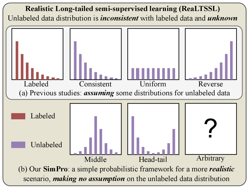
In response to these challenges, the concept of realistic long-tailed semi-supervised learning (ReaLTSSL), which aims at addressing the unknown and mismatched class distributions, has garnered significant attention (Kim et al., 2020; Wei et al., 2021; Oh et al., 2022; Wei & Gan, 2023). Notably, recent works ACR (Wei & Gan, 2023) and CPE (Ma et al., 2024) pre-define anchor distributions for unlabeled data (Fig. 1 (a)). The ACR estimates the distributional distance to adapt consistency regularization, while CPE involves training multiple classifiers, each tailored to a specific class distribution. However, this approach presupposes certain knowledge about the unlabeled data distribution, preventing its applications in real-world scenarios where anchor distributions may not represent all possible distributions. Furthermore, the prevailing techniques often employ multi-branch frameworks and introduce additional loss functions, adding complexity and limiting their generality.
To address these limitations, we propose a Simple Probabilistic (SimPro) framework for ReaLTSSL. We revisit pseudo-label-based SSL techniques through the lens of the Expectation-Maximization (EM) algorithm. The EM algorithm, a well-known iterative method in statistical modeling, is particularly relevant in SSL for handling unobserved latent variables, such as pseudo-labels of unlabeled data. The E-step entails generating pseudo-labels with the model, while the M-step involves model training using both labeled and unlabeled data. In the context of unknown and mismatched class distributions, the E-step may produce biased pseudo-labels, diminishing the algorithm’s effectiveness. Our SimPro avoids fixed assumptions about the unlabeled data distribution, instead of innovatively extending the EM algorithm for ReaLTSSL. Specifically, we explicitly decouple the modeling of conditional and marginal distributions. Such separation enables a closed-form solution for the marginal distribution in the M step. Subsequently, this solution is employed to train a Bayes classifier. This Bayes classifier, in turn, improves the quality of pseudo-labels generated in the E-step. Not only does SimPro offer high effectiveness, but it is also easy to implement, requiring minimal code modifications.
Moreover, we expand upon existing evaluation methods (Oh et al., 2022), which primarily focus on three known class distributions (consistent, uniform, and reversed), by introducing two novel realistic scenarios: middle and head-tail distributions (Fig. 1 (b)). The middle distribution represents a concentration of classes in the middle range of labeled data’s classes, whereas the head-tail distribution indicates a concentration at both extremes. Notably, our method is theoretically general enough to handle any other distribution patterns, since no prior assumptions are required.
We summarize our contributions as follows:
1. We present SimPro, a simple probabilistic framework tailored for realistic long-tailed semi-supervised learning. This framework does not presuppose any knowledge about the class distribution of unlabeled data. It hinges on the explicit estimation and utilization of class distributions within the EM algorithm. SimPro effectively mitigates the challenges posed by unknown and mismatched class distributions, stepping towards a more realistic LTSSL scenario.
2. We introduce two novel class distribution patterns for unlabeled data, complementing the existing three standard ones. This expansion facilitates a more comprehensive and realistic evaluation of ReaLTSSL algorithms, bridging the gap between theoretical models and practical applications.
3. Comprehensive experiments on five commonly used benchmarks (CIFAR10/100-LT, STL10-LT, and ImageNet-127/1k) and five distinct class distributions validate that our SimPro consistently achieves SOTA performance.
2 Related Work
Semi-supervised learning (SSL) has gained prominence through a subset of algorithms that use unlabeled data to enhance model performance. This enhancement primarily occurs through the generation of pseudo-labels, effectively forming a self-training loop (Miyato et al., 2018; Berthelot et al., 2019a, b; Huang & Du, 2022; Wang et al., 2023). Modern SSL methodologies, such as those presented in (Berthelot et al., 2019a; Sohn et al., 2020), integrate pseudo-labeling with consistency regularization. This integration fosters uniform predictions across varying representations of a single image, thereby bolstering the robustness of deep networks. A notable example, FixMatch (Sohn et al., 2020), has demonstrated exceptional results in image recognition tasks, outperforming competing SSL approaches.
The efficacy of SSL algorithms heavily relies on the quality of the pseudo-labels they generate. However, both labeled and unlabeled data follow a long-tailed class distribution in the LTSSL scenario. Conventional SSL methods are prone to produce biased pseudo-labels, which significantly downgrade their effectiveness.
Long-tailed semi-supervised learning has garnered considerable interest due to its relevance in numerous real-world applications. In this domain, DARP (Kim et al., 2020) and CReST (Wei et al., 2021) aim to mitigate the issue of biased pseudo-labels by aligning them with the class distribution of labeled data. Another notable approach (Lee et al., 2021) employs an auxiliary balanced classifier, which is trained through the down-sampling of majority classes, to enhance generalization capabilities. These algorithms have markedly improved performance but operate under the assumption of identical class distributions for labeled and unlabeled data.
In addressing Realistic LTSSL challenges, DASO (Oh et al., 2022) innovates by adapting the proportion of linear and semantic pseudo-labels to the unknown class distribution of unlabeled data. Its success largely depends on the discriminative quality of the representations, a factor that becomes less reliable in long-tailed distributions. ACR (Wei & Gan, 2023), on the other hand, attempts to refine consistency regularization by pre-defining distribution anchors and achieves promising results. CPE (Ma et al., 2024) trains multiple anchor experts where each is tasked to model one distribution. However, such anchor distribution-based approaches might not encompass all potential class distribution scenarios, and their complexity could hinder the broader application.
3 Method
In this section, we first introduce the problem formulation of ReaLTSSL (Sec. 3.1), setting the stage for our method. Subsequently, we delve into the proposed simple and probabilistic framework, SimPro (Sec. 3.2). We provide implementation details in Sec. 3.3 to elucidate SimPro further.
3.1 Preliminaries
Problem formulation.
We begin by outlining the formulation for the realistic long-tailed semi-supervised learning (ReaLTSSL) problem, laying the groundwork for our approach. The setup involves a labeled dataset and an unlabeled dataset , where represents the -th data sample and is the corresponding one-hot label, with denoting the number of classes. The objective of ReaLTSSL is to train a classifier , parameterized by .
Assumption 1.
We assume a realistic scenario where labeled, unlabeled, and test data share the same conditional distribution , yet may exhibit distinct marginal distributions . Crucially, the marginal distribution of the unlabeled data remains unknown.
Further, we consider five diverse distributions for the unlabeled data (Fig. 1), reflecting various real-world situations.
The EM algorithm in semi-supervised learning.
In SSL, pseudo-labeling is a key technique for leveraging unlabeled data. This involves creating pseudo-labels for the unlabeled data using the model and then training the model with both the pseudo-labeled and ground-truth data. This aligns with the Expectation-Maximization (EM) algorithm (Dempster et al., 1977), where the E-step generates pseudo-labels, and the M-step updates the parameters using the pseudo-labels, maximizing the likelihood function.
Our method builds on a popular algorithm FixMatch (Sohn et al., 2020), which integrates consistency regularization in the standard SSL setting. Pseudo-labels are created via weakly-augmented unlabeled data and applied to train strongly-augmented samples based on a confidence threshold. The loss for unlabeled data is
| (1) |
where and represent the prediction logits for weakly and strongly augmented samples, respectively, denotes the cross-entropy loss, and is the confidence threshold.
Long-tailed learning.
In typical SSL scenarios, the assumption of identical distributions for labeled, unlabeled, and test data often prevails. However, long-tailed learning tasks usually involve imbalanced training sets and balanced test sets, leading to discrepancies in the prior distribution of between training and testing data. Some studies (Ren et al., 2020; Menon et al., 2021; Hong et al., 2021) tackle this via Bayesian inference, introducing a prior distribution over class labels:
| (2) |
where denotes the class frequency in the training or test set, is the class distribution parameter and is the parameter of . Here we omit the parameter of for simplicity. The detailed mathematical derivation is provided in App. A.
While supervised learning allows for a known distribution parameter , enabling a direct application to model and explicit decoupling from , ReaLTSSL poses a greater challenge as the prior for unlabeled data is unknown. This necessitates innovative approaches to adapt to the imbalanced data while maintaining model efficacy.
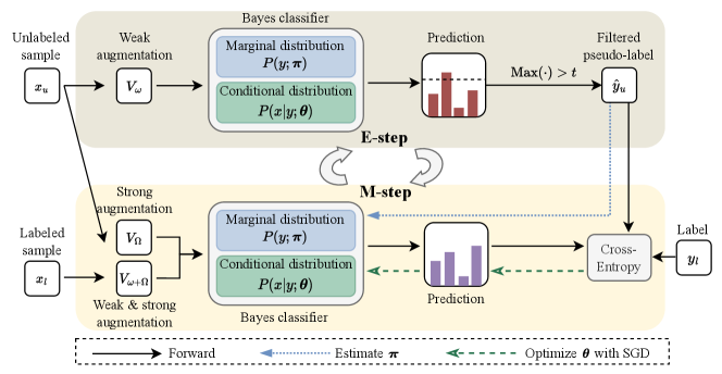
3.2 SimPro Framework
Framework overview.
In the realistic semi-supervised learning (ReaLTSSL) context, the conventional assumption of independent and identically distributed (i.i.d.) labeled and unlabeled data is no longer valid. Moreover, the marginal (class) distribution of the unlabeled data may be inconsistent with that of the labeled data and remains unknown, which challenges the traditional SSL frameworks.
To overcome this, we introduce SimPro, an elegant and effective probabilistic framework adapted for the unique ReaLTSSL setting. Illustrated in Fig. 2, SimPro distinctively decouples and , unlike traditional SSL methods (Sohn et al., 2020). In the E-step, we generate pseudo-labels using the parameters and obtained from the previous M-step. The M-step then models the conditional distribution using network parameters , which are optimized through gradient descent. Simultaneously, we derive a closed-form solution for the class distribution , represented by .
Probabilistic model.
In addressing the ReaLTSSL challenge, we adopt an Expectation-Maximization (EM) approach, underpinned by a robust probabilistic model. The model is governed by the fundamental principles of conditional probability, as shown in:
| (3) |
Here, we do not explicitly parameterize , as per the independence of parameters through conditional parameterization (Koller & Friedman, 2009). Thus, when is not a condition, the parameters of the relevant notions omit the parameters of , such as , , , etc. According to Sec. 3.1, this may lead to a potential misunderstanding, as the equation seems to suggest that is parameterized by and , which is not the case. The detailed mathematical derivation is provided in App. A.
We focus on estimating the parameters and , pivotal for learning a discriminative model. Consequently, we concentrate on those terms dependent on and , sidelining those independent of these parameters.
The complete data log-likelihood is thus articulated as:
| (4) |
where signifies the class distributions for labeled and unlabeled data, respectively, with and representing the number of labeled/unlabeled samples.
E-step (generating pseudo-labels).
By Eq. 4, the expected complete data log-likelihood function is derived from the preceding iteration’s parameters, and :
| (5) | ||||
The E-step involves generating soft pseudo-labels under the current and . These soft pseudo-labels are specifically defined by Eq. 10, which is detailed in Prop. 2. In the subsequent M-step, these pseudo-labels are used alongside the one-hot labels of the labeled data to compute the cross-entropy loss.
M-step (optimizing and ).
The M-step focuses on optimizing the expected complete data log-likelihood -function concerning the parameters and .
(a) Optimization of : The closed-form solution for can be derived directly from the -function (Eq. 5). Specifically, the terms involving in are given by
| (6) |
Proposition 1 (Closed-form Solution for ).
The optimal that maximizes is
| (7) |
(b) Optimization of : The network parameters , unlike which have a closed-form solution, are optimized using standard stochastic gradient descent (SGD). Combining with Sec. 3.1, the terms involving in are
| (8) | ||||
which simplifies to the supervised scenario in Sec. 3.1 by treating as soft labels. Maximizing Eq. 8 corresponds to minimizing the cross-entropy loss. Here, is interpreted as the estimated overall frequency of class . The optimization of model parameters using the overall frequency vector is crucial for learning a Bayes classifier.
Proposition 2 (Bayes Classifier).
In conjunction with the high-confidence filtering (Eq. 1), the optimal for learning a Bayes classifier is mathematically derived as:
| (9) |
Subsequently, with the model parameter which is optimized using the , the corresponding Bayes classifier for unlabeled or test dataset with estimated or uniform class distribution is defined by the equation:
| (10) | ||||
| (11) |
Building upon Prop. 2, it is crucial to acknowledge that the parameter vector is vital for learning Bayes classifiers. Consequently, to delve deeper into the theoretical foundations, we evaluate the impact of on the model’s performance. In line with the principles of online decision theory, we establish a regret bound for the decision error rate on the test set, denoted as . Our analysis is simplified by concentrating on a binary classification scenario, where the labels belong to .
Proposition 3 (Regret Bound).
Let denote the vector obtained in Eq. 9 when pseudo-labels are replaced by ground-truth labels. For the decision error rate on the test set, the regret bound is expressed as:
| (12) |
where .
Prop. 3 illustrates that the regret bound is primarily governed by the first-order term of the estimation deviation. Additionally, it is inversely proportional to the ground truth , highlighting the learning challenges associated with imbalanced training data from a regret-bound perspective.
| consistent | uniform | reversed | middle | head-tail | ||||||
| FixMatch (Sohn et al., 2020) | 62.90.36 | 67.81.13 | 67.62.56 | 73.03.81 | 59.90.82 | 62.50.94 | 64.30.63 | 71.70.46 | 58.31.46 | 66.60.87 |
| w/ CReST+ (Wei et al., 2021) | 67.50.45 | 76.30.86 | 74.90.80 | 82.21.53 | 62.01.18 | 62.91.39 | 58.50.68 | 71.40.60 | 59.30.72 | 67.20.48 |
| w/ DASO (Oh et al., 2022) | 70.11.81 | 76.00.37 | 83.10.47 | 86.60.84 | 64.00.11 | 71.00.95 | 69.00.31 | 73.10.68 | 70.50.59 | 71.10.32 |
| w/ ACR† (Wei & Gan, 2023) | 70.90.37 | 76.10.42 | 91.90.02 | 92.50.19 | 83.20.39 | 85.20.12 | 73.80.83 | 79.30.30 | 77.60.20 | 79.30.48 |
| w/ SimPro | 74.20.90 | 80.70.30 | 93.60.08 | 93.80.10 | 83.50.95 | 85.80.48 | 82.60.38 | 84.80.54 | 81.00.27 | 83.00.36 |
| CIFAR100-LT () | STL10-LT () | |||||||
|---|---|---|---|---|---|---|---|---|
| consistent | uniform | reversed | middle | head-tail | ||||
| FixMatch (Sohn et al., 2020) | 40.00.96 | 39.61.16 | 36.20.63 | 39.70.61 | 38.20.82 | FixMatch (Sohn et al., 2020) | 72.40.71 | 64.02.27 |
| w/ CReST+ (Wei et al., 2021) | 40.11.28 | 37.60.88 | 32.40.08 | 36.90.57 | 35.11.10 | w/ CReST+ (Wei et al., 2021) | 71.50.96 | 68.51.88 |
| w/ DASO (Oh et al., 2022) | 43.00.15 | 49.40.93 | 44.10.25 | 43.11.20 | 43.80.43 | w/ DASO (Oh et al., 2022) | 78.40.80 | 75.30.44 |
| w/ ACR† (Wei & Gan, 2023) | 40.70.57 | 50.20.82 | 44.10.14 | 42.40.47 | 41.10.09 | w/ ACR (Wei & Gan, 2023) | 83.00.32 | 81.50.25 |
| w/ SimPro | 43.10.40 | 52.20.16 | 45.50.34 | 43.60.35 | 44.80.56 | w/ SimPro | 84.50.39 | 82.50.25 |
3.3 Implementation Details
Training objective for optimizing .
In SimPro, the E-step primarily involves generating pseudo-labels using parameters and . Consequently, in the M-step, we first focus on optimizing the network parameter guided by Eq. 8 via Stochastic Gradient Descent (SGD). Building on the FixMatch algorithm (Sohn et al., 2020), the overall training objective is formulated as:
| (13) |
where and represent the losses on labeled and unlabeled data, respectively. The hyper-parameter acts as a scaling factor, the specifics of which are elucidated later.
For , we modify it (originally the standard cross-entropy loss) following Eq. 8:
| (14) |
where is a hyper-parameter for enhancing adaptability to long-tail distributions (Menon et al., 2021). is batch size.
For , we implement the standard SSL format (Eq. 1) and adapt it for ReaLTSSL:
| (15) |
where controls the number of unlabeled samples, and is a confidence threshold. The pseudo-label of weak augmentation from the Bayes classifier (Eq. 10) is denoted by
| (16) |
and the actual prediction is obtained using strong augmentation and calibrated with as shown in Eq. 8:
| (17) |
Moreover, in practical situations, the size of the unlabeled dataset is generally larger than that of the labeled dataset . To ensure a balanced sample size in each iteration, we usually set in Eq. 15. In specific scenarios, we further adjust the balance factor in Eq. 13 to . This methodology effectively mitigates overfitting to the labeled data (see Tabs. 6 and 7).
Closed-form solution of .
Extended EM algorithm and pseudo-code.
Based on the previous analysis, Our SimPro framework can be summarized as an extended EM algorithm, which includes:
E-step (Eq. 10): Generating pseudo-labels using model parameters and estimated distribution parameters ;
M-step: Optimizing network parameters via SGD using Eq. 8 (actually using Eq. 13), and solving distribution parameters and hyper-parameters by Eq. 7 and Eq. 9.
For further clarity, the pseudo-code of SimPro is provided in Alg. 1. The modifications we made to the core training code, in comparison to FixMatch, are highlighted in bold. In the SimPro, we incorporate just a single additional line of code in the M-step to compute the closed-form solution of (Prop. 1). Furthermore, only four lines of code need to be modified to construct a Bayes classifier (Prop. 2) and to balance the loss between labeled and unlabeled data (denoted as ). These minor yet crucial adjustments demonstrate that our SimPro framework is not only grounded in rigorous theoretical derivation but is also straightforward to implement in practice, exemplifying both simplicity and elegance.
4 Experiments
In this section, we first present the main results on various ReaLTSSL benchmarks in Sec. 4.1. More analysis, including the ablation studies and the visualization results, is presented in Sec. 4.2 to further evaluate the effectiveness of our SimPro. For detailed information regarding the experimental setup, please refer to App. B.
| ImageNet-127 | ||
|---|---|---|
| FixMatch (Sohn et al., 2020) | 29.7 | 42.3 |
| w/ DARP (Kim et al., 2020) | 30.5 | 42.5 |
| w/ CReST+ (Wei et al., 2021) | 32.5 | 44.7 |
| w/ CoSSL (Fan et al., 2022) | 43.7 | 53.9 |
| w/ ACR (Wei & Gan, 2023) | 57.2 | 63.6 |
| w/ SimPro | 59.1 | 67.0 |
| ImageNet-127 | ||
| FixMatch (Sohn et al., 2020) | 38.7 | 46.7 |
| w/ ACR† (Wei & Gan, 2023) | 49.5 | 56.1 |
| w/ ACR (Wei & Gan, 2023) | 50.6 | 57.3 |
| w/ SimPro | 55.7 | 63.8 |
| ImageNet-1k | ||
| FixMatch (Sohn et al., 2020) | – | – |
| w/ ACR† (Wei & Gan, 2023) | 13.2 | 23.4 |
| w/ ACR (Wei & Gan, 2023) | 13.8 | 23.3 |
| w/ SimPro | 19.7 | 25.0 |
4.1 Results
We first conduct experiments on the four representative benchmark datasets with different class imbalance ratios. We denote the class imbalance ratio of labeled, unlabeled, and test data as , , and , respectively. Our method is compared with five competitive baseline approaches, i.e., FixMatch (Sohn et al., 2020), CReST+ (Wei et al., 2021), DASO (Oh et al., 2022), ACR (Wei & Gan, 2023), and CPE (Ma et al., 2024). Note that for a fair comparison, we first compare with ACR in the ReaLTSSL setting, where the unlabeled class distribution is unknown and inaccessible. Specifically, we compare our vanilla SimPro with ACR’s variant that removes its pre-defined anchor distributions, denoted as ACR†. Then we implement SimPro⋆ by also alleviating the anchor distributions in our SimPro framework, comparing SimPro⋆ with the original ACR and CPE.
Main results and comparison with SOTA baselines.
The results are presented in Tab. 1 (for CIFAR10-LT), Tab. 2 (for CIFAR100-LT and STL10-LT), and Tab. 3 (for ImageNet-127/1k). It can be concluded that our method consistently outperforms the competitors across all distributions of unlabeled data and achieves SOTA performance. Notably, SimPro exhibits significant performance improvements on our two newly introduced distributions of unlabeled data: middle and head-tail. This substantiates the robust generalization capabilities of SimPro across various distributions that could potentially appear in real-world scenarios.
It is worth noting that compared to CIFAR10/100-LT, STL10-LT is a more challenging dataset that mirrors the real-world data distribution scenarios: an unknown distribution for the unlabeled data. The results in Tab. 2 demonstrate the significant improvements of SimPro over baseline methods.
Moreover, we also conduct experiments on ImageNet-127, whose test dataset is imbalanced and consistent with the labeled data and unlabeled data. However, this is not suitable as a benchmark for long-tail learning, as biased classifiers tend to perform well in such scenarios, which is precisely what we aim to avoid. Therefore, we resample it to achieve a uniform test distribution (). The results highlight that our SimPro achieves substantial performance enhancements when evaluated against this balanced test dataset. Beyond this, we further conduct experiments on ImageNet-1k to validate the performance of our method across a broader range of classes. The results in Tab. 3 demonstrate that our SimPro achieves state-of-the-art performance on ImageNet-1k.
| consistent | uniform | reversed | middle | head-tail | |
|---|---|---|---|---|---|
| CPE | 76.8 | 81.0 | 80.8 | – | – |
| ACR | 77.0 | 91.3 | 81.8 | 77.9 | 79.0 |
| SimPro | 74.2 | 93.6 | 83.5 | 82.6 | 81.0 |
| SimPro⋆ | 80.0 | 94.1 | 85.0 | – | – |
The results of SimPro⋆ using anchor distributions.
To investigate the impact of the anchor distributions in ACR and CPE (Ma et al., 2024), we also incorporate them into our approach, referred to as SimPro⋆. Instead of calculating the distribution distance and adjusting the consistency regularization as in ACR or employing multiple anchor experts as in CPE, our usage of these anchors is more straightforward: after training for five epochs, we calculate the distance between our estimated distribution and the three anchor distributions (i.e. consistent, uniform, and reversed). This calculation helps us predict the actual distribution and construct the Bayes classifier. Then we fix the marginal distribution parameters in the remainder of the training.
The results in Tab. 4 indicate that (1) the usage of anchor distributions can significantly enhance the performance of SimPro⋆, consistently outperforming the original ACR and CPE; (2) our estimation for is accurate (Fig. 5 further validates the accurate estimation of ); (3) when the pre-defined anchors fail to cover the evaluated distributions (middle and head-tail), SimPro outperforms ACR by a large margin; (4) even compared to the original ACR, SimPro exhibits enhanced performance across all scenarios except the consistent distribution. This demonstrates the superior robustness and generalization ability of our method. We believe these advantages guarantee a better adaptable nature for SimPro in real applications and are more valuable than the accuracy improvements when using the anchor distributions.
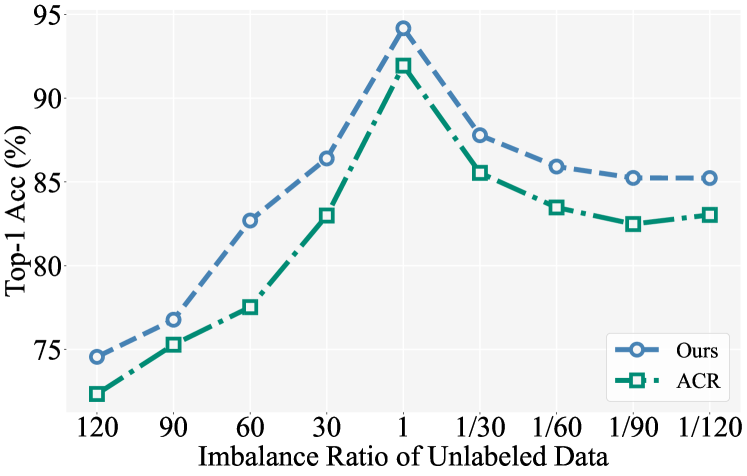
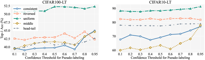
Evaluation under more imbalance ratios.
Fig. 3 reports the performance of SimPro under more imbalance ratios of unlabeled data. The results indicate that our method consistently outperforms ACR across all imbalance ratios, further substantiating the robustness of our method.
| Distribution Estimation | ||||||
|---|---|---|---|---|---|---|
| E-step | M step | consistent | uniform | reversed | middle | head-tail |
| ✗ | ✗ | 40.7 | 35.3 | 43.2 | 27.1 | 47.7 |
| ✗ | ✓ | 64.1 | 92.6 | 78.6 | 64.9 | 74.8 |
| ✓ | ✓ | 74.2 | 93.6 | 83.5 | 82.6 | 81.0 |
4.2 Analysis
Ablation Study.
| consistent | reversed | middle | head-tail | ||
|---|---|---|---|---|---|
| FixMatch | ✗ | 62.9 | 59.9 | 64.3 | 58.3 |
| ✓ | 40.7 | 43.2 | 27.1 | 47.7 | |
| w/ ACR | ✗ | 70.9 | 83.2 | 73.8 | 77.6 |
| ✓ | 68.7 | 58.9 | 69.7 | 72.4 | |
| w/ SimPro | ✗ | 52.7 | 78.8 | 58.8 | 71.5 |
| ✓ | 75.2 | 83.5 | 82.6 | 81.0 |
| CIFAR10-LT () | CIFAR100-LT () | STL10-LT ( N/A) | |||
| ✗ | 92.1 | 91.2 | 49.4 | 76.4 | 80.0 |
| ✓ | 93.6 | 93.8 | 52.2 | 83.0 | 85.2 |
We conduct a series of ablation studies to validate the effectiveness of different components in SimPro.
(a) Marginal distribution estimation. We first investigate the impact of the estimation for (M-step, Prop. 1) and its usage in building the Bayes classifier for pseudo-label generation (E-step, Prop. 2). The results in Tab. 5 substantiate the high effectiveness and the necessity of this estimation in driving the success of our approach, thereby validating our methodology both theoretically and practically.
(b) More unlabeled samples (larger ) in each iteration. As mentioned in the experimental setup, we manually set the ratio between unlabeled and labeled samples in each training iteration as (Eq. 15). In ACR or Fixmatch, this ratio is set as . To investigate the impact of this adjustment, we adopt our setting of for ACR and Fixmatch. The results in Tab. 6 demonstrate that our method can effectively leverage the unlabeled data for a more accurate estimation of the marginal distribution parameters . However, the baseline methods suffer from an imbalanced number of labeled/unlabeled samples, because of the absence of our Bayes classifier derived in Prop. 2.
(b) Scaling factor . As elucidated in Sec. 3.3, we introduce a scaling factor (Eq. 13) to mitigate the risk of overfitting. This measure is primarily due to memory and training environment limitations, which restrict the feasible batch size and , when . In the test configurations detailed in Tab. 7, the ratio is about for CIFAR and for STL10-LT. An insufficient results in a disproportionately high number of labeled data within a mini-batch, potentially leading to overfitting. Hence, we incorporate the to balance the losses between labeled and unlabeled data. Our empirical findings demonstrate that the use of this simple parameter can significantly enhance model performance, particularly STL10-LT, where there is a substantial disparity between the sizes of labeled and unlabeled data.
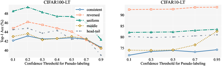
Hyperparameter Sensitivity.
As outlined in App. B, we discover that reducing the threshold value improves performance for the CIFAR100-LT dataset. The rationale behind adjusting the confidence threshold is based on the observation that an increase in the number of classes typically results in a corresponding decrease in the confidence of the predictions. Consequently, it becomes necessary to lower the threshold to accommodate this change in confidence levels. Sensitivity analysis regarding the threshold value is presented in Fig. 4. It is consistently observed across different settings that the optimal performance is achieved when the threshold is set at and for the CIFAR100-LT and CIFAR10-LT, respectively. Moreover, to compare with ACR, we also conduct a sensitivity analysis of the confidence threshold for ACR. The results in Fig. 6 of App. C demonstrate that lowering the threshold does not improve performance for ACR.
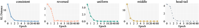
Visualization of Estimation Quality.
Our study includes a visualization of the estimated distribution quality in Fig. 5. The vertical axis quantifies the Kullback-Leibler (KL) divergence, which measures the deviation of the estimated distribution from the ground truth. The results indicate a significant improvement in estimation accuracy after only a few training epochs. This empirical evidence validates the effectiveness of the theoretically derived estimation method of distribution, as outlined in Prop. 1.
5 Conclusion
In this paper, we introduce SimPro, a novel probabilistic framework for realistic long-tailed semi-supervised learning (ReaLTSSL). This framework represents a pioneering advancement in the field by innovatively enhancing the Expectation-Maximization (EM) algorithm. The key innovation lies in the explicit separation of the estimation process for conditional and marginal distributions. In the M-step, this separation allows for the derivation of a closed-form solution for the marginal distribution parameters. Additionally, SimPro optimizes the parameters of the conditional distribution via gradient descent, facilitating the learning of a Bayes classifier. In the E-step. the Bayes classifier, in turn, generates high-quality pseudo-labels. SimPro is characterized by its elegant theoretical underpinnings and its ease of implementation, which requires only minimal modifications to existing codebases. Furthermore, we incorporate two innovative class distributions specifically for unlabeled data. These distributions provide a more comprehensive and realistic evaluation of ReaLTSSL algorithms. Empirical evidence from various benchmarks demonstrates that SimPro consistently delivers state-of-the-art performance, highlighting its robustness and superior generalization capabilities.
Acknowledgements
This work was supported in part by the National Key R&D Program of China under Grant 2021ZD0140407, in part by the National Natural Science Foundation of China under Grants 62276150, 62321005 and 42327901.
Impact Statement
This paper presents work whose goal is to advance the field of Machine Learning. There are many potential societal consequences of our work, none which we feel must be specifically highlighted here.
References
- Berthelot et al. (2019a) Berthelot, D., Carlini, N., Cubuk, E. D., Kurakin, A., Sohn, K., Zhang, H., and Raffel, C. Remixmatch: Semi-supervised learning with distribution alignment and augmentation anchoring. arXiv preprint, 2019a.
- Berthelot et al. (2019b) Berthelot, D., Carlini, N., Goodfellow, I., Papernot, N., Oliver, A., and Raffel, C. A. Mixmatch: A holistic approach to semi-supervised learning. In NeurIPS, 2019b.
- Coates et al. (2011) Coates, A., Ng, A., and Lee, H. An analysis of single-layer networks in unsupervised feature learning. In AISTATS, volume 15, pp. 215–223. PMLR, 2011.
- Dempster et al. (1977) Dempster, A. P., Laird, N. M., and Rubin, D. B. Maximum likelihood from incomplete data via the em algorithm. Journal of the royal statistical society: series B (methodological), 39(1):1–22, 1977.
- Deng et al. (2009) Deng, J., Dong, W., Socher, R., Li, L.-J., Li, K., and Fei-Fei, L. Imagenet: A large-scale hierarchical image database. In CVPR, 2009.
- Du et al. (2024) Du, C., Wang, Y., Song, S., and Huang, G. Probabilistic contrastive learning for long-tailed visual recognition. TPAMI, 2024.
- Fan et al. (2022) Fan, Y., Dai, D., Kukleva, A., and Schiele, B. Cossl: Co-learning of representation and classifier for imbalanced semi-supervised learning. In CVPR, 2022.
- He et al. (2016) He, K., Zhang, X., Ren, S., and Sun, J. Deep residual learning for image recognition. In CVPR, 2016.
- Hong et al. (2021) Hong, Y., Han, S., Choi, K., Seo, S., Kim, B., and Chang, B. Disentangling label distribution for long-tailed visual recognition. In CVPR, 2021.
- Huang & Du (2022) Huang, G. and Du, C. The high separation probability assumption for semi-supervised learning. IEEE Transactions on Systems, Man, and Cybernetics: Systems, 52(12):7561–7573, 2022.
- Kang et al. (2020) Kang, B., Xie, S., Rohrbach, M., Yan, Z., Gordo, A., Feng, J., and Kalantidis, Y. Decoupling representation and classifier for long-tailed recognition. In ICLR, 2020.
- Kim et al. (2020) Kim, J., Hur, Y., Park, S., Yang, E., Hwang, S. J., and Shin, J. Distribution aligning refinery of pseudo-label for imbalanced semi-supervised learning. In NeurIPS, 2020.
- Koller & Friedman (2009) Koller, D. and Friedman, N. Probabilistic graphical models: principles and techniques. MIT press, 2009.
- Krizhevsky et al. (2009) Krizhevsky, A., Hinton, G., et al. Learning multiple layers of features from tiny images. 2009.
- Lai et al. (2022) Lai, Z., Wang, C., Gunawan, H., Cheung, S.-C. S., and Chuah, C.-N. Smoothed adaptive weighting for imbalanced semi-supervised learning: Improve reliability against unknown distribution data. In ICML, 2022.
- Lee et al. (2013) Lee, D.-H. et al. Pseudo-label: The simple and efficient semi-supervised learning method for deep neural networks. In Workshop on challenges in representation learning, ICML, volume 3, pp. 896. Atlanta, 2013.
- Lee et al. (2021) Lee, H., Shin, S., and Kim, H. Abc: Auxiliary balanced classifier for class-imbalanced semi-supervised learning. In NeurIPS, 2021.
- Liu et al. (2019) Liu, Z., Miao, Z., Zhan, X., Wang, J., Gong, B., and Yu, S. X. Large-scale long-tailed recognition in an open world. In CVPR, 2019.
- Loshchilov & Hutter (2017) Loshchilov, I. and Hutter, F. Sgdr: Stochastic gradient descent with warm restarts. In ICLR, 2017.
- Ma et al. (2024) Ma, C., Elezi, I., Deng, J., Dong, W., and Xu, C. Three heads are better than one: Complementary experts for long-tailed semi-supervised learning. In AAAI, 2024.
- Menon et al. (2021) Menon, A. K., Jayasumana, S., Rawat, A. S., Jain, H., Veit, A., and Kumar, S. Long-tail learning via logit adjustment. In ICLR, 2021.
- Miyato et al. (2018) Miyato, T., Maeda, S.-i., Koyama, M., and Ishii, S. Virtual adversarial training: a regularization method for supervised and semi-supervised learning. TPAMI, 2018.
- Oh et al. (2022) Oh, Y., Kim, D.-J., and Kweon, I. S. DASO: Distribution-aware semantics-oriented pseudo-label for imbalanced semi-supervised learning. In CVPR, 2022.
- Ren et al. (2020) Ren, J., Yu, C., Ma, X., Zhao, H., and Yi, S. Balanced meta-softmax for long-tailed visual recognition. In NeurIPS, 2020.
- Sohn et al. (2020) Sohn, K., Berthelot, D., Carlini, N., Zhang, Z., Zhang, H., Raffel, C. A., Cubuk, E. D., Kurakin, A., and Li, C.-L. FixMatch: Simplifying semi-supervised learning with consistency and confidence. In NeurIPS, 2020.
- Tarvainen & Valpola (2017) Tarvainen, A. and Valpola, H. Mean teachers are better role models: Weight-averaged consistency targets improve semi-supervised deep learning results. In NeurIPS, 2017.
- Wang et al. (2023) Wang, Y., Guo, J., Wang, J., Wu, C., Song, S., and Huang, G. Erratum to meta-semi: A meta-learning approach for semi-supervised learning. CAAI Artificial Intelligence Research, 2023.
- Wei et al. (2021) Wei, C., Sohn, K., Mellina, C., Yuille, A., and Yang, F. CReST: A class-rebalancing self-training framework for imbalanced semi-supervised learning. In CVPR, 2021.
- Wei & Gan (2023) Wei, T. and Gan, K. Towards realistic long-tailed semi-supervised learning: Consistency is all you need. In CVPR, 2023.
- Wei et al. (2022) Wei, T., Liu, Q.-Y., Shi, J.-X., Tu, W.-W., and Guo, L.-Z. Transfer and share: semi-supervised learning from long-tailed data. Machine Learning, pp. 1–18, 2022.
- Zagoruyko & Komodakis (2016) Zagoruyko, S. and Komodakis, N. Wide residual networks. In Procedings of the British Machine Vision Conference 2016. British Machine Vision Association, 2016.
Appendix A Details of the Probabilistic Model
We provide a detailed derivation and analysis to demonstrate that the probabilistic model is correctly defined with an explicit parameterization of . Given the independence of parameters through conditional parameterization (Koller & Friedman, 2009), we can decompose the joint probability distribution as follows:
| (18) |
Applying Bayes’ rule, we obtain:
| (19) |
It is evident that and appear only on the left and right sides of the equation, respectively, indicating that the equation is neither a function of nor but is parameterized solely by . We define the above equation as , that is:
| (20) |
Returning to the equation in the main paper, we have:
| (21) |
Although we explicitly parameterize , it is clear that is parameterized solely by and , and is independent of . In fact, the fitting target of the network parameters is .
Since we did not explicitly parameterize in our framework, when is not a condition, the parameters of the relevant notions omit the parameters of , such as , , , etc. This may lead to a potential misunderstanding, as:
| (22) |
suggests that seems to be parameterized by and . However, if we recover the omitted parameter of , we have:
| (23) |
which is consistent with the explicit parameterization of .
Therefore, the probabilistic model is correctly defined without the explicit parameterization of .
Appendix B Experimental Setup
Datasets.
To validate the effectiveness of SimPro, we employ five commonly used SSL datasets, CIFAR10/100 (Krizhevsky et al., 2009), STL10 (Coates et al., 2011), ImageNet-127 (Fan et al., 2022) and orginal ImageNet-1k (Deng et al., 2009). Following the methodology described in ACR (Wei & Gan, 2023), we denote the number of samples for each category in the labeled, unlabeled dataset as , , respectively, where are the class indices. We define , , and as the class imbalance ratios for labeled, unlabeled, and test data, respectively. We specify ‘LT’ for those imbalanced variants. These ratios are calculated as and . The sample number of the -th class follows an exponential distribution, expressed as for labeled and for unlabeled data.
As illustrated in Fig. 1, for the CIFAR10/100 datasets, we constructed five class distributions to test the performance of different algorithms under more general settings. Regarding the STL10 dataset, due to the unknown ground-truth labels of the unlabeled data, we approach the experiments by controlling the imbalance ratio of the labeled data.
For ImageNet-127, we follow the original setting in Fan et al. (2022) (). Nevertheless, this approach does not serve as an appropriate benchmark for long-tail learning. In these scenarios, biased classifiers often exhibit high performance, which is exactly the outcome we seek to prevent. Consequently, we also resample the test dataset to ensure a uniform distribution (). Following Fan et al. (2022), we reduce the image resolution to and in response to resource constraints.
Training hyper-parameters.
Our experimental setup mainly follows FixMatch (Sohn et al., 2020) and ACR (Wei & Gan, 2023). For example, we employ the Wide ResNet-28-2 (Zagoruyko & Komodakis, 2016) on CIFAR10/100 and STL10, and ResNet-50 (He et al., 2016) on ImageNet-127. All models are optimized with SGD. Several settings are slightly different from those in ACR: as outlined in Sec. 3.3, to achieve a balanced training, we set the ratio between unlabeled and labeled samples in each batch as ( on CIFAR, on STL10-LT, and on ImageNet-127, ), where are the total sample numbers of unlabeled/labeled data. In contrast, is set as for all datasets in ACR. The effectiveness of this adjustment is validated in Tab. 6.
The batch size for labeled data is on CIFAR10/100 and STL10-LT, and on ImageNet-127. To ensure a fair comparison, the training epochs are reduced to on CIFAR10/100 and STL10-LT, and on ImageNet-127. The initial learning rate is linearly scaled to on CIFAR10/100 and STL10-LT, and on ImageNet-127, which decays with a cosine schedule (Loshchilov & Hutter, 2017) as in ACR.
Regarding the hyperparameter used in Eq. 14, we follow the guidelines from Menon et al. (2021) and set and for CIFAR10-LT/STL10-LT and CIFAR100-LT/ImageNet-127, respectively.
For the confidence threshold in Eq. 1), we set on CIFAR10-LT/STL10-LT following Sohn et al. (2020). We adjust it to on CIFAR100-LT/Imagenet-127, as we observe that reducing the threshold enhances performance (Fig. 4).
Specifically, the settings on ImageNet-1k are identical to those on ImageNet-127.
Appendix C More Experimental Results
| consistent | uniform | reversed | middle | head-tail | |
| ACR | 81.6 | 92.1 | 85.0 | 73.6 | 79.8 |
| SimPro | 80.7 | 93.8 | 85.8 | 84.8 | 83.0 |
| SimPro⋆ | 82.7 | 94.3 | 86.0 | – | – |
| consistent | uniform | reversed | middle | head-tail | |
| ACR | 44.9 | 52.2 | 42.3 | 42.6 | 42.6 |
| SimPro | 43.1 | 52.3 | 45.5 | 43.6 | 44.8 |
| SimPro⋆ | 45.9 | 53.8 | 46.0 | – | – |
Appendix D Proof of Proposition 1
Proof.
We employ the method of Lagrange multipliers to find the optimal values of and that maximize the function subject to the constraints of probability distributions (i.e., the elements of and must sum to 1). Let and be the Lagrange multipliers for these constraints. The Lagrangian can be formulated as 111 is the one-hot label, but when is the subscript of a variable, it represents the -th category, that is, . we omit this difference without affecting the understanding.:
| (24) |
The partial derivatives of with respect to and are calculated as follows:
| (25) | ||||
| (26) |
Due to fact that is a categorical distribution, the derivatives are:
| (27) | ||||
| (28) |
Setting these partial derivatives to zero and solving for and :
| (29) | ||||
| (30) |
Applying the constraint that the sum of probabilities equals 1, we get:
| (31) | ||||
| (32) |
Therefore, the optimal solutions are:
| (33) |
∎
Appendix E Proof of Proposition 2
Proof.
We structure our proof in two parts: First, we validate the proposition when training exclusively with labeled data. Then, we extend our analysis to include scenarios incorporating unlabeled data. This approach stems from our threshold-based strategy for filtering low-confidence pseudo labels in the training process. Initially, only labeled data are used, gradually integrating unlabeled data as training progresses.
Case 1: Labeled Data Only
Our proof begins by revisiting the definition of with respect to :
| (34) |
Ignoring the constant term, maximizing is equivalent to minimizing the empirical risk:
| (35) |
The empirical risk serves as an approximation of the expected risk, with denoting the distribution of labeled data:
| (36) |
where is defined as:
| (37) |
With the non-negativity and zero-equality conditions of KL divergence, minimizing the expected risk implies:
| (38) |
We aim to validate the Bayes classifier:
| (39) |
which leads to the formulation:
| (40) |
Integrating Eq. 38 with Eq. 40 yields:
| (41) |
Summing over in Eq. 41 leads to:
| (42) |
Substituting Eq. 42 into Eq. 41 results in:
| (43) |
As the constant becomes irrelevant in the logarithmic term of , in light of Prop. 1, we deduce the optimal :
| (44) |
Case 2: Labeled and Unlabeled Data
Expanding our proof to include both labeled and unlabeled data, our optimization objective remains consistent: maximizing by minimizing the empirical risk:
| (45) |
This risk approximates the expected risk over :
| (46) |
where represents the mixture distribution of both labeled and unlabeled data and its density is:
| (47) |
Acknowledging that is a Bayes classifier, we conclude:
| (48) |
which leads to the formulation:
| (49) |
Following the same logic as in the labeled data case:
| (50) |
This results in:
| (51) |
In accordance with Prop. 1, we determine the optimal as:
| (52) |
∎
Appendix F Proof of Proposition 3
Proof.
We begin by examining . The decision error rate is mathematically defined as follows:
| (53) |
This formulation quantifies the error in decision-making by integrating the conditional error rates across all possible outcomes.
Building upon the Bayes optimal classifier as outlined in Eq. 11, the posterior probability essential for decision-making on the test set is expressed as:
| (54) |
Here, represents the model’s discriminative function, parameterized by , for decision outcome given an input .
The ground truth distribution, as approximated by parameters and , is denoted by and , respectively. The formal relationship between the estimated and true distributions is expressed as follows:
| (55) |
indicating a proportional relationship between the model’s estimation and the true data distribution.
Integrating the formulation of posterior probability with the relationship between estimated and true distributions allows us to derive the following expression:
| (56) |
where the final step is justified by the fact that the class distribution in the test set is uniform.
The decision criterion is thus formulated as:
| (57) |
where
| (58) |
We assume without loss of generality, due to the symmetric nature of the decision problem.
The decision error rate is then expressed as:
| (59) |
Minimizing the decision error rate is achieved when , leading to the Bayes decision error rate, which is the theoretical lower bound of error rates across all possible distributions.
| (60) |
Finally, comparing with the optimal decision error rate, we explore the difference:
| (61) |
where the final inequality is justified by the condition that due to .
∎