Simulating bicycle traffic by the Intelligent-Driver Model – reproducing the traffic-wave characteristics observed in a bicycle-following experiment
Abstract
Bicycle traffic operations become increasingly important and yet are largely ignored in the traffic flow community, until recently. We hypothesize that there is no qualitative difference between vehicular and bicycle traffic flow dynamics, so the latter can be described by reparameterized car-following models. To test this proposition, we reproduce bicycle experiments on a ring with the Intelligent-Driver Model and compare its fit quality (calibration) and predictive power (validation) with that of the Necessary-Deceleration-Model which is specifically designed for bike traffic. We find similar quality metrics for both models, so the above hypothesis of a qualitative equivalence cannot be rejected.
1 Introduction
In spite of its growing relevance, past research on bicycle traffic operations in experiments Navin1994bikeExperiments ; Taylor1999bikeOperationsReview ; Andresen2014_universal ; Jiang2016traffic and models Gould2009bikeCA ; Andresen2014_NDM ; Jin2015improved is remarkably scarce. In contrast, there is a multitude of empirical and experimental investigations for vehicular traffic flow, as well as a plethora of models (for an overview see, e.g., TreiberKesting-Book ). Therefore, it is natural to ask whether there is a significant qualitative difference between vehicular and bicycle traffic flow at all. In other words, the question arises if one can use the well-developed car-following models for the simulation of bicycle traffic instead of creating new bicycle models.
In this paper, we test the Intelligent Driver Models (IDM) Treiber2000_PRE as a typical representative of car-following models against the ”ring-road” bicycle traffic experiments of Erik Andresen et. al. Andresen2014_NDM ; Andresen2014_universal . In addition, we compare the IDM fit quality with that of a specifically designed “bicycle-following model”, the Necessary-Deceleration-Model (NDM) Andresen2014_NDM .
2 Models under Investigation
Two microscopic car-following models are considered – the IDM Treiber2000_PRE and the NDM Andresen2014_NDM . Both of them are formulated as coupled ordinary differential equations and characterized by an acceleration function which depends on the actual speed , the approaching rate to the leader, and the gap .
The IDM is defined by the acceleration function Treiber2000_PRE
| (1) |
where is the dynamically desired gap. The IDM contains five parameters to identify via calibration – . Recently, it has been found that stochasticity plays a significant role for low-speed traffic flow, so we have added the simplest form of white acceleration noise to the acceleration equation (see Treiber2017stochIDM_TRB for details) when simulating collective effects, cf. Sec. 5.4.
The NDM is originally formulated in terms of difference equations for the speed Andresen2014_NDM which, in the limit of update times tending to zero, is equivalent to a coupled differential equation with the acceleration function
| (2) |
where
| (3) |
| (4) |
| (5) |
The safety distance is a linear function of the cyclist’s speed , is a length of the cyclist. The NDM has 5 parameters to calibrate – .
3 Ring-road Experiment
Trajectory data of bicycle experiments were considered for calibration and validation. These experiments were conducted by the University of Wuppertal in cooperation with Jülich Forschungszentrum on 6th of May, 2012 Andresen2014_NDM . Cyclists were moving one after another along the oval track of 86 m length. However the measuring area covered only a straight line of 20 m length. Group experiments were performed for several density levels – 5, 7, 10, 18, 20 and 33 participants.
Recently, further experiments with up to 63 cyclists have been performed Jiang2016traffic giving essentially the same results and showing even more pronounced stop-and-go waves for the higher densities.
4 Methods
We have estimated the model performance by two approaches. One is based on trajectories, and the other on aggregated properties of scatter plots derived from stationary measurements (virtual detectors).
4.1 Calibrating and Validating Trajectories
Pairs of consecutive trajectories were used for calibration and validation according to the global approach TreiberKesting-Book ; Kurtc2016 . Specifically, the microscopic model was initialized with the empirically given speed and gap , and the trajectory of the following cyclist for a given leader trajectory was calculated using the ballistic update (see Chapter 10.2 of TreiberKesting-Book ) with a time step . Afterwards, the simulated gaps were compared with the experimentally observed gaps by means of two objective functions, namely the absolute error measure
| (6) |
and the relative error measure
| (7) |
4.2 Comparing Microscopic Fundamental Diagrams
We used virtual stationary detectors at several positions of the ring and calculated
-
•
the instantaneous speed of cyclist at passage time,
-
•
the ”microscopic density” , i.e., the inverse space headway to the leader at passage time,
-
•
and the microscopic flow , i.e., the inverse (time) headway.
We combined these data to microscopic speed-density scatter plots both for the simulations and the experiments by defining the sets and , respectively. In order to quantitatively compare the similarity, we create a partitioning of the data points by filtering them according to equally-spaced density intervals,
| (8) |
where . The key idea is to interpret as a one-dimensional random variable. Now we calculate the (cumulative) distribution functions both for the experiment, , and the simulations, , and calculate the Kolmogorov-Smirnov distance
| (9) |
The distance averaged over all density bins provides the quantitative metric which estimates the similarity of two data-clouds
| (10) |
5 Results
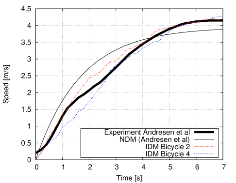
5.1 Free acceleration
First, we compare and calibrate the free acceleration profile against the experimental results (cf. Fig. 4 of Andresen2014_NDM ). After calibrating the relevant IDM parameters to the values and and adding a small amaount of white noise (intensity ), we found a better agreement compared to the NDM (Fig. 1).
5.2 Collective Driving Behavior
Both models have been calibrated for all trajectory pairs and optimal parameter value distributions were obtained. Table 5.2 presents the calibration errors. For both error measures (Eq. 6 and 7) lower error values correspond to the IDM whereas higher errors come from the NDM.
The use of several error measures can be interpreted as a benchmark for the robustness of the model calibration. Specifically, for a good model, the calibration results and the distribution of the calibrated parameters should not significantly vary with the chosen error measure. We compare the Kolmogorov-Smirnov distance
| (11) |
of the distributions and of parameter as obtained by calibrating the trajectories with respect to the absolute and relative error measure and , respectively. According to the results presented in Table 5.2, the IDM tends to be slightly more robust than the NDM.
| \svhline Model | ||
|---|---|---|
| IDM | 2.86 | 3.01 |
| NDM | 4.85 | 5.05 |
| \svhline |
| \svhline IDM | |||||
|---|---|---|---|---|---|
| 0.023 | 0.027 | 0.036 | 0.029 | ||
| \svhline NDM | |||||
| 0.043 | 0.035 | 0.072 | 0.026 | 0.039 | |
| \svhline |
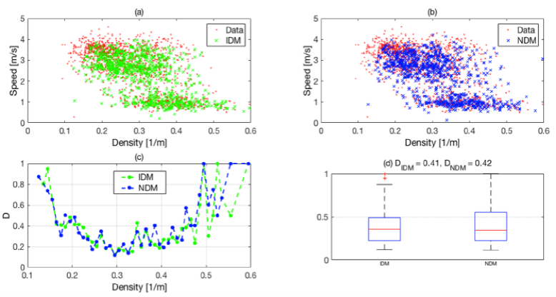
5.3 Microscopic Fundamental Diagrams Comparison
We have calculated the microscopic fundamental diagram and the distance measures both for the real data and for the simulation of the two models with the optimal parameter values without noise. The results are shown in Fig. 2.
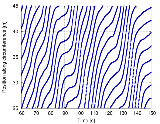
5.4 Stop-and-go waves
Besides calibrating the IDM by trajectory pair, we also tested if the IDM can produce collective effects such as the stop-and-go traffic observed in the experiments Andresen2014_NDM and Jiang2016traffic . Figure 3 shows the result. Instead of using heterogeneous drivers, we simplified the investigation as much as possible by using a single parameter set for all drivers replacing the heterogeneity by white acceleration noise. In contrast to the free-flow simulation (Fig. 1), a higher amount of was needed to approximatively reproduce the observed amplitude and frequency statistics of the traffic waves while the free-flow parameters and were the same. The calibrated values , , and were near the median of the trajectory-by-trajectory calibration of Section 5.2.
5.5 Inter-Driver Variation and Validation
Validation by cross comparison implies determining the error measures for a certain test data set by simulating the model with the parameters calibrated to the disjunct “learning” data set TreiberKesting-Book . For each experiment (5, 10, 15, 18, 20 and 33 participants, respectively), we have separately calculated the calibration-validation matrix whose elements give the error measure for the trajectory pair as obtained from the model calibrated to the trajectory pair . The diagonal element are the calibration errors whereas the off-diagonal elements , , give a superposition of the validation error and the inter-driver variation of follower with respect to follower . The average validation error and calibration error are given by
| (12) |
| (13) |
where is a number of trajectory pairs. Notice that a separation of these two causes would require using disjunct parts of the same trajectory for calibration and validation which is only viable for longer trajectories than the available ones. To obtain measures for the overall fitting quality and the predictive power plus inter-driver variations, we have calculated the ratio of the average validation error to the calibration error (Table 5.5).
| \svhline | ||||||
| IDM | ||||||
| Calibration error | 1.74 | 3.08 | 2.87 | 11.98 | 3.43 | 5.67 |
| Validation error | 32.23 | 26.37 | 22.53 | 32.79 | 26.6 | 32.63 |
| Ratio | 18.5 | 8.5 | 7.8 | 2.7 | 7.7 | 5.7 |
| NDM | ||||||
| Calibration error | 1.28 | 6.39 | 3.49 | 3.54 | 5.78 | 7.43 |
| Validation error | 42.58 | 32.51 | 29.19 | 35.58 | 31.67 | 27.58 |
| Ratio | 33.2 | 5.1 | 8.3 | 10.0 | 5.5 | 3.7 |
| \svhline |
6 Discussion and Conclusions
According to the results presented in this paper, we conclude that the IDM, which has a similar underlying heuristics as the NDM, can not only describe vehicular but also bicycle traffic, or, at least, ”bicycle following”.The IDM trajectories fit even better to the data than that of the NDM. The IDM calibration errors with absolute and relative error measures are 2.86 and 3.01 % whereas for the NDM they are 4.85 and 5.05 % respectively. The application of several objective functions indicates that the IDM calibration is also more robust in comparison to the NDM. Validation results show that the predictive power of the IDM is better than that of the NDM. However, the validation results are confounded by discrepancies from inter-driver variations, so further investigations to separate these factors are necessary.
The analysis of macroscopic characteristics such as speed-density relations provides more or less the same results for both models. Specifically, the averaged Kolmogorov distance (Eq. 10) is nearly the same. Furthermore, the stochastic IDM can well describe the statistical features of the amplitude and frequency of the observed stop-and-go waves. We conclude that the dynamics of bicycle traffic differs only quantitatively from vehicular traffic and reparameterized car-following models such as the IDM work at least as well as dedicated “bike-following” models.
References
- (1) Andresen, E., Chraibi, M., Seyfried, A., Huber, F.: Basic Driving Dynamics of Cyclists, pp. 18–32. Springer Berlin Heidelberg, Berlin, Heidelberg (2014)
- (2) Gould, G., Karner, A.: Modeling bicycle facility operation: cellular automaton approach. Transportation Research Record: Journal of the Transportation Research Board (2140), 157–164 (2009)
- (3) Jiang, R., Hu, M.B., Wu, Q.S., Song, W.G.: Traffic dynamics of bicycle flow: Experiment and modeling. Transportation Science (2016)
- (4) Jin, S., Qu, X., Xu, C., Ma, D., Wang, D.: An improved multi-value cellular automata model for heterogeneous bicycle traffic flow. Physics Letters A 379(39), 2409–2416 (2015)
- (5) Kurtc, V., Treiber, M.: Calibrating the local and platoon dynamics of car-following models on the reconstructed ngsim data. In: Traffic and Granular Flow’15, pp. 515–522. Springer (2016)
- (6) Navin, F.P.: Bicycle traffic flow characteristics: experimental results and comparisons. ITE journal 64(3), 31–37 (1994)
- (7) Taylor, D., Davis, W.: Review of basic research in bicycle traffic science, traffic operations, and facility design. Transportation Research Record: Journal of the Transportation Research Board (1674), 102–110 (1999)
- (8) Treiber, M., Henneke, A., Helbing, D.: Congested traffic states in empirical observations and microscopic simulations. Physical Review E 62(2), 1805–1824 (2000)
- (9) Treiber, M., Kesting, A.: Traffic Flow Dynamics: Data, Models and Simulation. Springer, Berlin (2013). URL http://www.traffic-flow-dynamics.org
- (10) Treiber, M., Kesting, A.: The intelligent driver model with stochasticity-new insights into traffic flow oscillations. Transportation Research Part B (2017). DOI 10.1016/j.trb.2017.08.012. URL http://dx.doi.org/10.1016/j.trb.2017.08.012
- (11) Zhang, J., Mehner, W., Holl, S., Boltes, M., Andresen, E., Schadschneider, A., Seyfried, A.: Universal flow-density relation of single-file bicycle, pedestrian and car motion. Physics Letters A 378(44), 3274–3277 (2014)