Simulating Diffusion Bridges with Score Matching
Abstract
We consider the problem of simulating diffusion bridges, which are diffusion processes that are conditioned to initialize and terminate at two given states. The simulation of diffusion bridges has applications in diverse scientific fields and plays a crucial role in the statistical inference of discretely-observed diffusions. This is known to be a challenging problem that has received much attention in the last two decades. This article contributes to this rich body of literature by presenting a new avenue to obtain diffusion bridge approximations. Our approach is based on a backward time representation of a diffusion bridge, which may be simulated if one can time-reverse the unconditioned diffusion. We introduce a variational formulation to learn this time-reversal with function approximation and rely on a score matching method to circumvent intractability. Another iteration of our proposed methodology approximates the Doob’s -transform defining the forward time representation of a diffusion bridge. We discuss algorithmic considerations and extensions, and present numerical results on an Ornstein–Uhlenbeck process, a model from financial econometrics for interest rates, and a model from genetics for cell differentiation and development to illustrate the effectiveness of our approach.
Keywords: Diffusion; Diffusion bridge; Score matching; Stochastic differential equation; Time-reversal.
1 Introduction
Diffusion processes have been used extensively in mathematical and natural sciences. A diffusion process in is defined by the stochastic differential equation
| (1) |
where is a drift function, is a diffusion coefficient, and is a -dimensional Brownian motion. We suppose and are sufficiently regular to induce a unique weak solution and is uniformly positive definite for all . For any , we denote the transition density of (1) with respect to the Lebesgue measure on as and assume that it is positive for ease of exposition. While the numerical simulation of can be routinely handled by time-discretization schemes (Kloeden and Platen, 1992), the task of simulating initialized at and conditioned to terminate at is a challenging problem that has received much attention in the last two decades.
Simulating the conditioned process , commonly referred to as a diffusion bridge, has applications in diverse fields such as computational chemistry (Bolhuis et al., 2002; Wang et al., 2020), financial econometrics (Elerian et al., 2001; Durham and Gallant, 2002), genetics (Wang et al., 2011), and shape analysis (Arnaudon et al., 2022). When performing statistical inference for parameters of and in the case where is observed at discrete time points, diffusion bridge simulation is a crucial tool that allows one to impute missing paths between observations within an expectation-maximization algorithm or a Gibbs sampler (Pedersen, 1995; Roberts and Stramer, 2001; Eraker, 2001; Beskos et al., 2006; Golightly and Wilkinson, 2008; van der Meulen and Schauer, 2017).
By Doob’s -transform (Rogers and Williams, 2000, p. 83), it is well-known that satisfies
| (2) |
where and denotes the gradient operator. The term forces the conditioned process towards the terminal condition . As the transition density and hence its logarithmic gradient is intractable for most diffusions, exploiting this result to simulate diffusion bridges is highly non-trivial. To this end, one can characterize as the solution of the backward Kolmogorov equation
| (3) |
with terminal condition at time given by the Dirac measure at , where denotes the generator of (Stroock and Varadhan, 1997). Equation (3) reveals that propagates information about the terminal constraint backwards in time. However, numerical resolution of this partial differential equation is particularly challenging due to the singularity at time , and computationally demanding when the dimension is large (Wang et al., 2020). Furthermore, one must run a solver for every pair of conditioned states considered.
A common approach to address these difficulties is to simulate a proposal bridge process , satisfying with . One constructs using a tractable approximation of (2), and corrects for the discrepancy using importance sampling or an independent Metropolis–Hastings algorithm (Papaspiliopoulos and Roberts, 2012; Elerian et al., 2001). The simple choice typically performs poorly as it does not take the constraint into account (Pedersen, 1995). The drift of a Brownian bridge has been considered in several works (Durham and Gallant, 2002; Delyon and Hu, 2006; Stramer and Yan, 2007; Papaspiliopoulos et al., 2013), and improved by Whitaker et al. (2017) using an innovative decomposition of the process into deterministic and stochastic parts. Clark (1990) followed by Delyon and Hu (2006) studied the choice that incorporates the dynamics of the original process . To introduce more flexibility and better mimic the structure of (2), Schauer et al. (2017) proposed setting , where is an analytically tractable transition density of an auxiliary process. For tractability, the latter is typically chosen from the class of linear processes and can be optimized to get the best approximation within this class (van der Meulen and Schauer, 2017). Other Markov chain Monte Carlo approaches include Gibbs sampling (Eraker, 2001), Langevin-type stochastic partial differential equations (Stuart et al., 2004; Beskos et al., 2008), piecewise deterministic Monte Carlo (Bierkens et al., 2021), and manifold Hamiltonian Monte Carlo methods (Graham et al., 2022).
The exact simulation algorithms developed in Beskos and Roberts (2005) and Beskos et al. (2006) can be employed to sample diffusion bridges without any time-discretization error. However, these elegant methods are limited to the class of diffusion processes that can be transformed to have unit diffusion coefficient. Bladt and Sørensen (2014) and Bladt et al. (2016) devised an ingenious methodology to simulate diffusion bridges based on coupling and time-reversal of diffusions. Their proposed method is applicable to the class of ergodic diffusions with an invariant density that is either explicitly known or numerically approximated. Closely related approaches include sequential Monte Carlo algorithms that resample using backward information filter approximations (Guarniero, 2017), information from backward pilot paths (Lin et al., 2010), or guided weight functions (Del Moral and Murray, 2015). The main idea underlying these works is the representation of the diffusion bridge in (2) and (3).
2 Diffusion bridges
2.1 Time-reversed bridge process
It can be shown that the time-reversed bridge process satisfies
| (4) |
with drift function , another standard Brownian motion , , and is the divergence of . Here denotes the score of the marginal density of the diffusion bridge process at time . We refer readers to Haussmann and Pardoux (1986), Millet et al. (1989), and Cattiaux et al. (2023) for conditions under which the representation in (4) holds. By the Markov property, we have the relation
| (5) |
as . This implies that is simply the score of the transition density of .
Exploiting this backward time representation to derive diffusion bridge approximations is also highly non-trivial due to the intractability of the transition density , which is now characterized by the forward Kolmogorov equation , with initial condition at time given by the Dirac measure at and denotes the Fokker–Planck operator of (Stroock and Varadhan, 1997). Numerical resolution of using partial differential equation solvers also suffers from the same difficulties as (3). A key observation is that (4) can be understood as first setting to satisfy the terminal constraint, and then evolving using the time-reversal of (1). Due to the influence of the score , the process will end at the initial constraint by construction. This connection between simulation of a diffusion bridge and time-reversal of its original diffusion process will form the basis of our score approximation. We refer readers to Section B of the Supplementary Material for an alternative and more elementary argument to establish this connection.
2.2 Learning time-reversal with score matching
We introduce a variational formulation to learn the time-reversal of (1), involving path measures on the space of continuous functions from to , equipped with the cylinder -algebra. Consider the time-reversed process satisfying
| (6) |
with drift function that mimics the form of in (4). Here represents a function approximation of the score that depends on parameters to be optimized. We shall measure the score approximation error as
| (7) |
where denotes expectation with respect to the path measure induced by in (1) with , and denotes the Euclidean norm weighted by a positive definite .
Let be the path measure induced by the parameterised forward process . We consider minimizing the Kullback–Leibler divergence , where denotes the Radon–Nikodym derivative of with respect . The following result gives an upper bound of this objective and shows that the process will end at the initial constraint if the score approximation error is finite.
Proposition 1.
Assuming , we have and holds -almost surely.
Under Novikov’s condition, an exponential integrability assumption, Girsanov’s theorem shows that (Le Gall, 2016a, Theorem 5.22, Theorem 4.13). We do not provide here any assumption on to guarantee that . Previous work by Delyon and Hu (2006) and Schauer et al. (2017) have studied necessary conditions for the law of a proposal bridge process and the law of the diffusion bridge to be equivalent. These findings suggest that the behaviour of should be as , which can be used to guide our parameterization of the score approximation. For example, we consider where denotes a bounded function.
Although Proposition 1 clearly relates the approximation of the time-reversal of (1) to the approximation of the score , its form is not amenable to optimization. The following result gives an alternative and practical expression by adapting the idea of denoising score matching (Vincent, 2011) to our setting.
Proposition 2.
For any partition of the interval , we have if , where is a constant independent of , the loss function is defined as
| (8) |
and for and .
Therefore minimizing the Kullback–Leibler divergence is equivalent to minimizing the loss function . This allows us to circumvent the intractable score by working with , the score of the transition density . Although the latter is also intractable, approximations can be made when the sub-interval is sufficiently small. For example, under the Euler–Maruyama scheme (Kloeden and Platen, 1992, p. 340) with stepsize ,
Hence the loss can be approximated and minimized using stochastic gradient algorithms by simulating time-discretized paths under (1). The minimal loss of , achieved when -almost surely, is unknown as the constant is typically intractable. After obtaining the score approximation , we can simulate a proposal bridge from (6) with and correct it using importance sampling or independent Metropolis–Hastings. Time-discretization considerations and proposal correction procedures are detailed in Section C of the Supplementary Material.
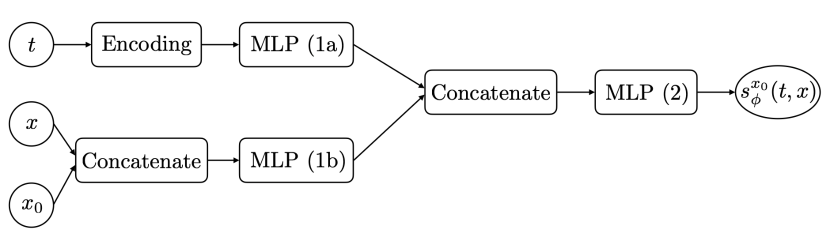
In scenarios where one is interested in multiple pairs of conditioned states , we can extend the above methodology to avoid having to learn multiple score approximations as follows. We let the score approximation in (6) also depend on the initial condition , and average the Kullback–Leibler objective with a distribution on that can be sampled from. By applying the arguments of Proposition 2 conditionally on , we obtain a loss function given by averaging (8) over , which can be minimized using time-discretization and stochastic gradient algorithms. In this setting, we parameterize the score approximation as , where is now a function that also depends on the initial condition .
2.3 Learning Doob’s -transform
It is instructive to consider the time-reversal of (4), which gives
| (9) |
with drift function . Using the form of and the relation , we can rewrite as
| (10) |
and recover the Doob’s -transform in (2). Although this is to be expected as the reversal of the time-reversed process should recover the original process, it forms the basis of our approximation of (2).
After obtaining an approximation of , another iteration of our methodology can be used to obtain a function approximation of . For brevity, this is detailed in Section 2.3 of the Supplementary Material. Plugging in both approximations in (10) then gives an approximation of , which could be of interest in algorithms where one requires a forward time representation of the proposal bridge process (Lin et al., 2010; Del Moral and Murray, 2015). However, this comes at the cost of learning two approximations and some accumulation of errors. Recent work by Baker et al. (2024) have extended our approach to directly approximate , which is not necessarily the score of a probability density.
3 Related work on generative modeling
Denoising diffusion models are popular state-of-the-art generative models (Sohl-Dickstein et al., 2015; Song et al., 2021). These models are based on a diffusion process that transforms data into random normal noise. Their time-reversal is then approximated to obtain a generative model that maps sampled noise to synthetic data. Recent extensions have generalized these models to allow the distribution at the terminal time to be arbitrary rather than a normal distribution (De Bortoli et al., 2021; Vargas et al., 2021; Chen et al., 2022). While there are similarities between these methods and our proposed methodology, the challenges in simulating a diffusion bridge between two states and are distinctly different. Firstly, the diffusion process in (1) usually represents a probabilistic model for a problem of interest with an intractable transition density. In contrast, denoising diffusion models employ an Ornstein–Uhlenbeck process, leveraging its analytically tractable transition density to learn the score. Secondly, while the time dimension in (1) arises from modeling time series data, with the time interval representing the time between observations, the time variable in denoising diffusion models is artificially introduced and represents the time necessary for the diffusion to transform the data distribution into a normal distribution. Thirdly, the time-reversed process (4) is initialized from a conditioned state in our setting, whereas it is initialized from a normal distribution in generative models.
4 Numerical examples
4.1 Preliminaries
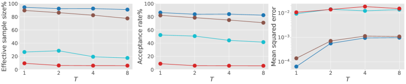
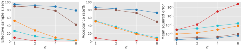
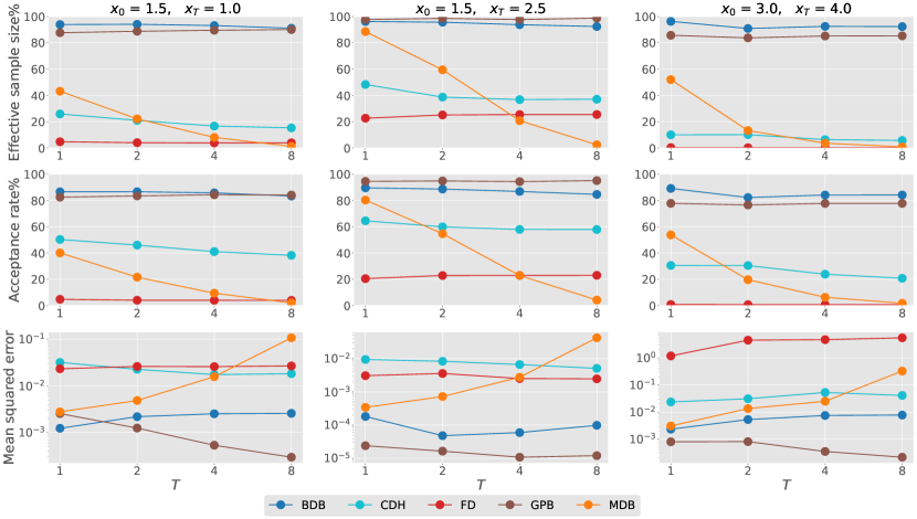
As our methodology allows one to employ any function approximator, we harness the flexibility of neural networks and the ease of implementation using modern software to approximate score functions. We adopt the parameterization of the score approximation in Section 2.2 with defined by a neural network. The choice of neural network and stochastic gradient algorithm is detailed in Section D.2 of the Supplementary Material. Optimization times ranged between several seconds to a few minutes on a simple desktop machine and can be reduced with hardware accelerators. As such computational overheads are marginal when deploying proposal bridge processes within an independent Metropolis–Hastings algorithm with many iterations or an importance sampler with many samples, we focus on assessing the quality of our proposals in settings where existing proposal methods are unsatisfactory. The performance measures considered are the acceptance rate of independent Metropolis–Hastings, and in the case of an importance sampling estimator of , the effective sample size proportion, and the variance var or the mean squared error when the true transition density is known. More implementation details are described in Section D of the Supplementary Material. These measures were computed using samples or iterations, and independent repetitions of each method. We benchmark our approximations of the backward diffusion bridge (BDB) and forward diffusion bridge (FDB) in (4) and (9) against the Clark–Delyon–Hu (CDH) proposal bridge studied by Clark (1990) and Delyon and Hu (2006), the forward diffusion (FD) of Pedersen (1995), the guided proposal bridge (GPB) by Schauer et al. (2017), and the modified diffusion bridge (MDB) of Durham and Gallant (2002). Given the difficulty of comparing the wide range of methods for diffusion bridges in a completely fair manner, as their strengths and weaknesses can depend on the specificities of the problem under consideration, we note that our objective is merely to illustrate a new avenue to improve the construction of proposal bridge processes. A Python package to reproduce all numerical results is available online222https://github.com/jeremyhengjm/DiffusionBridge.
4.2 Ornstein–Uhlenbeck process
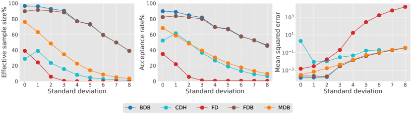
Consider (1) with linear drift function and identity diffusion coefficient . The transition density and score function are explicitly known and used as ground truth. The first and second rows of Fig. 1 illustrates the impact of the time horizon and dimension on algorithmic performance with the constraints . To study how performance degrades when we condition on rare states under the diffusion process , in the third row of Fig. 1, we set the initial state as and vary where the terminal state is in the tails of the transition density in multiples of its standard deviation.
We omit the guided proposal bridge in this example as it performs perfectly when its auxiliary process is the Ornstein–Uhlenbeck process. Our proposed methods offer substantial improvements over other methods without exploiting the correct parameterization. When comparing our forward and backward diffusion bridge approximations, we notice some accumulation of error, which is to be expected as the forward process is constructed using an additional score approximation. Given this observation, we will only consider the backward process in the following.
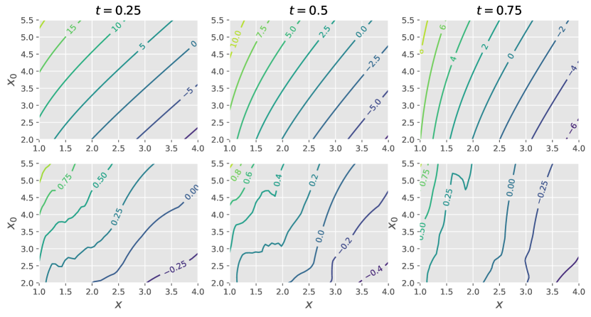
4.3 Interest rates model
We consider a special case of an interest rates model in Aït-Sahalia and Lo (1998), defined by (1) with and . This specification admits a tractable transition density and score function as ground truth, given in terms of modified Bessel functions and its derivative. For each , we first learn a single score approximation to handle multiple conditioned states by minimizing the loss in (8) averaged over initial states from the gamma distribution with shape and rate . We construct guided proposal bridges based on a first-order Taylor approximation of at the stable stationary point . We plot our score approximation error for in Fig. 2, and examine how algorithmic performance depends on and in Fig. 3. Our backward diffusion bridge approximation performs well for all considered and when conditioning requires the process to move away from the stationary point (first and third columns). Its performance is similar to guided proposal bridge and significantly better than other existing methods. While the performance of modified diffusion bridge typically degrades with , the results of forward diffusion and Clark–Delyon–Hu bridge depend on the specific conditioned states.
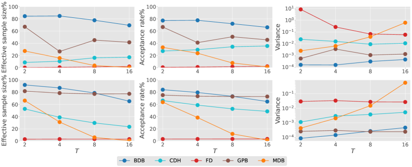
4.4 Cell model
We end with a cell differentiation and development model from Wang et al. (2011). Cellular expression levels of two genes are modelled by (1) with , where , for , describe self-activation, mutual inhibition and inactivation respectively, and captures intrinsic or external fluctuations. We consider the cell development from the undifferentiated state of to a differentiated state defined by another stable fixed point of satisfying . We employ an auxiliary Ornstein–Uhlenbeck process in the guided proposal bridge and optimize its parameters using the Kullback–Leibler divergence considered in Schauer et al. (2017). Fig. 4 displays the performance of all proposal methods to approximate this diffusion bridge. For this application, we observe improvement over guided proposal bridge when the diffusion coefficient is smaller, and significant improvement over other methods when the time horizon is long. These findings are consistent with numerical results obtained in Baker et al. (2024) for the same model.
5 Discussion
While implicit score matching (Hyvärinen, 2005) could have been an alternative to denoising score matching (Vincent, 2011), we found it to be less effective and computationally more expensive. If the terminal state is highly unlikely under the law of the unconditional diffusion, the score approximation learned using unconditional sample paths could be poor near . Nevertheless, we observed satisfactory experimental results for an Ornstein–Ulhenbeck process up to 8 standard deviations. In statistical problems where some hyperparameters of the diffusion are estimated using maximum likelihood or Bayesian inference, a direct application of our approach would require a new diffusion bridge approximation for each set of parameters considered. To avoid incurring significant computational cost, one could also incorporate parameter dependence in the score approximation procedure (Boserup et al., 2024). Recent work has also extended our approach to approximate directly without having to approximate a time-reversal (Baker et al., 2024) and to infinite-dimensional diffusion processes (Baker et al., 2024).
Acknowledgement
The authors thank the editor, associate editor, and reviewers for their comments, which have helped to improve the paper significantly. Arnaud Doucet and James Thornton were partially supported by the U.K. Engineering and Physical Sciences Research Council.
References
- Aït-Sahalia and Lo (1998) Aït-Sahalia, Y. and A. W. Lo (1998). Nonparametric estimation of state-price densities implicit in financial asset prices. The Journal of Finance 53(2), 499–547.
- Ambrosio et al. (2005) Ambrosio, L., N. Gigli, and G. Savaré (2005). Gradient Flows: in Metric Spaces and in the Space of Probability Measures. Birkhäuser.
- Andrieu et al. (2010) Andrieu, C., A. Doucet, and R. Holenstein (2010). Particle Markov chain Monte Carlo methods (with discussion). Journal of the Royal Statistical Society: Series B (Statistical Methodology) 72(3), 269–342.
- Arnaudon et al. (2022) Arnaudon, A., F. van der Meulen, M. Schauer, and S. Sommer (2022). Diffusion bridges for stochastic Hamiltonian systems and shape evolutions. SIAM Journal on Imaging Sciences 15(1), 293–323.
- Baker et al. (2024) Baker, E. L., M. Schauer, and S. Sommer (2024). Score matching for bridges without time-reversals. arXiv preprint arXiv:2407.15455.
- Baker et al. (2024) Baker, E. L., G. Yang, M. Severinsen, C. Hipsley, and S. Sommer (2024). Conditioning non-linear and infinite-dimensional diffusion processes. Advances in Neural Information Processing Systems 37, 10801–10826.
- Benton et al. (2024) Benton, J., V. De Bortoli, A. Doucet, and G. Deligiannidis (2024). Nearly -linear convergence bounds for diffusion models via stochastic localization. In The Twelfth International Conference on Learning Representations.
- Beskos et al. (2006) Beskos, A., O. Papaspiliopoulos, and G. O. Roberts (2006). Retrospective exact simulation of diffusion sample paths with applications. Bernoulli 12(6), 1077–1098.
- Beskos et al. (2006) Beskos, A., O. Papaspiliopoulos, G. O. Roberts, and P. Fearnhead (2006). Exact and computationally efficient likelihood-based estimation for discretely observed diffusion processes (with discussion). Journal of the Royal Statistical Society: Series B (Statistical Methodology) 68(3), 333–382.
- Beskos and Roberts (2005) Beskos, A. and G. O. Roberts (2005). Exact simulation of diffusions. The Annals of Applied Probability 15(4), 2422–2444.
- Beskos et al. (2008) Beskos, A., G. O. Roberts, A. Stuart, and J. Voss (2008). MCMC methods for diffusion bridges. Stochastics and Dynamics 8(03), 319–350.
- Bierkens et al. (2021) Bierkens, J., S. Grazzi, F. van der Meulen, and M. Schauer (2021). A piecewise deterministic Monte Carlo method for diffusion bridges. Statistics and Computing 31(3), 1–21.
- Bladt et al. (2016) Bladt, M., S. Finch, and M. Sørensen (2016). Simulation of multivariate diffusion bridges. Journal of the Royal Statistical Society: Series B (Statistical Methodology), 343–369.
- Bladt and Sørensen (2014) Bladt, M. and M. Sørensen (2014). Simple simulation of diffusion bridges with application to likelihood inference for diffusions. Bernoulli 20(2), 645–675.
- Bolhuis et al. (2002) Bolhuis, P. G., D. Chandler, C. Dellago, and P. L. Geissler (2002). Transition path sampling: Throwing ropes over rough mountain passes, in the dark. Annual Review of Physical Chemistry 53(1), 291–318.
- Boserup et al. (2024) Boserup, N., G. Yang, M. L. Severinsen, C. A. Hipsley, and S. Sommer (2024). Parameter inference via differentiable diffusion bridge importance sampling. arXiv preprint arXiv:2411.08993.
- Cattiaux et al. (2023) Cattiaux, P., G. Conforti, I. Gentil, and C. Léonard (2023). Time reversal of diffusion processes under a finite entropy condition. Annales de l’Institut Henri Poincare (B) Probabilites et statistiques 59(4), 1844–1881.
- Chen et al. (2022) Chen, S., S. Chewi, J. Li, Y. Li, A. Salim, and A. Zhang (2022). Sampling is as easy as learning the score: theory for diffusion models with minimal data assumptions. In The Eleventh International Conference on Learning Representations.
- Chen et al. (2022) Chen, T., G.-H. Liu, and E. Theodorou (2022). Likelihood training of Schrödinger bridge using forward-backward SDEs theory. In International Conference on Learning Representations.
- Clark (1990) Clark, J. M. C. (1990). The simulation of pinned diffusions. In 29th IEEE Conference on Decision and Control, pp. 1418–1420. IEEE.
- De Bortoli et al. (2021) De Bortoli, V., J. Thornton, J. Heng, and A. Doucet (2021). Diffusion Schrödinger bridge with applications to score-based generative modeling. In Advances in Neural Information Processing Systems. PMLR.
- Del Moral and Murray (2015) Del Moral, P. and L. M. Murray (2015). Sequential Monte Carlo with highly informative observations. SIAM/ASA Journal on Uncertainty Quantification 3(1), 969–997.
- Delyon and Hu (2006) Delyon, B. and Y. Hu (2006). Simulation of conditioned diffusion and application to parameter estimation. Stochastic Processes and their Applications 116(11), 1660–1675.
- Durham and Gallant (2002) Durham, G. B. and A. R. Gallant (2002). Numerical techniques for maximum likelihood estimation of continuous-time diffusion processes. Journal of Business & Economic Statistics 20(3), 297–338.
- Elerian et al. (2001) Elerian, O., S. Chib, and N. Shephard (2001). Likelihood inference for discretely observed nonlinear diffusions. Econometrica 69(4), 959–993.
- Eraker (2001) Eraker, B. (2001). MCMC analysis of diffusion models with application to finance. Journal of Business & Economic Statistics 19(2), 177–191.
- Golightly and Wilkinson (2008) Golightly, A. and D. J. Wilkinson (2008). Bayesian inference for nonlinear multivariate diffusion models observed with error. Computational Statistics & Data Analysis 52(3), 1674–1693.
- Graham et al. (2022) Graham, M. M., A. H. Thiery, and A. Beskos (2022). Manifold Markov chain Monte Carlo methods for Bayesian inference in diffusion models. Journal of the Royal Statistical Society Series B: Statistical Methodology 84(4), 1229–1256.
- Guarniero (2017) Guarniero, P. (2017). The Iterated Auxiliary Particle Filter and Applications to State Space Models and Diffusion Processes. Ph. D. thesis, University of Warwick.
- Haussmann and Pardoux (1986) Haussmann, U. G. and E. Pardoux (1986). Time reversal of diffusions. The Annals of Probability, 1188–1205.
- Hyvärinen (2005) Hyvärinen, A. (2005). Estimation of non-normalized statistical models by score matching. Journal of Machine Learning Research 6(4).
- Kingma and Ba (2014) Kingma, D. P. and J. Ba (2014). Adam: A method for stochastic optimization. arXiv preprint arXiv:1412.6980.
- Kloeden and Platen (1992) Kloeden, P. E. and E. Platen (1992). Stochastic differential equations. In Numerical Solution of Stochastic Differential Equations, pp. 103–160. Springer.
- Le Gall (2016a) Le Gall, J.-F. (2016a). Brownian Motion, Martingales, and Stochastic Calculus. Springer.
- Le Gall (2016b) Le Gall, J.-F. (2016b). Brownian Motion, Martingales, and Stochastic Calculus. Springer.
- Lin et al. (2010) Lin, M., R. Chen, and P. Mykland (2010). On generating Monte Carlo samples of continuous diffusion bridges. Journal of the American Statistical Association 105(490), 820–838.
- Middleton et al. (2019) Middleton, L., G. Deligiannidis, A. Doucet, and P. E. Jacob (2019). Unbiased smoothing using particle independent Metropolis–Hastings. In International Conference on Artificial Intelligence and Statistics. PMLR.
- Millet et al. (1989) Millet, A., D. Nualart, and M. Sanz (1989). Integration by parts and time reversal for diffusion processes. The Annals of Probability, 208–238.
- Papaspiliopoulos and Roberts (2012) Papaspiliopoulos, O. and G. O. Roberts (2012). Importance sampling techniques for estimation of diffusion models. In M. Kessler, A. Lindner, and M. Sorensen (Eds.), Statistical Methods for Stochastic Differential Equations, pp. 311–340. Chapman and Hall/CRC.
- Papaspiliopoulos et al. (2013) Papaspiliopoulos, O., G. O. Roberts, and O. Stramer (2013). Data augmentation for diffusions. Journal of Computational and Graphical Statistics 22(3), 665–688.
- Pedersen (1995) Pedersen, A. R. (1995). Consistency and asymptotic normality of an approximate maximum likelihood estimator for discretely observed diffusion processes. Bernoulli, 257–279.
- Roberts and Stramer (2001) Roberts, G. O. and O. Stramer (2001). On inference for partially observed nonlinear diffusion models using the Metropolis–Hastings algorithm. Biometrika 88(3), 603–621.
- Rogers and Williams (2000) Rogers, L. C. G. and D. Williams (2000). Diffusions, Markov processes and Martingales: Volume 2: Itô Calculus, Volume 2. Cambridge University Press.
- Schauer et al. (2017) Schauer, M., F. Van Der Meulen, and H. Van Zanten (2017). Guided proposals for simulating multi-dimensional diffusion bridges. Bernoulli 23(4A), 2917–2950.
- Sohl-Dickstein et al. (2015) Sohl-Dickstein, J., E. Weiss, N. Maheswaranathan, and S. Ganguli (2015). Deep unsupervised learning using nonequilibrium thermodynamics. In International Conference on Machine Learning, pp. 2256–2265. PMLR.
- Song and Kingma (2021) Song, Y. and D. P. Kingma (2021). How to train your energy-based models. arXiv preprint arXiv:2101.03288.
- Song et al. (2021) Song, Y., J. Sohl-Dickstein, D. P. Kingma, A. Kumar, S. Ermon, and B. Poole (2021). Score-based generative modeling through stochastic differential equations. In International Conference on Learning Representations.
- Stramer and Yan (2007) Stramer, O. and J. Yan (2007). On simulated likelihood of discretely observed diffusion processes and comparison to closed-form approximation. Journal of Computational and Graphical Statistics 16(3), 672–691.
- Stroock and Varadhan (1997) Stroock, D. W. and S. S. Varadhan (1997). Multidimensional Diffusion Processes, Volume 233. Springer Science & Business Media.
- Stuart et al. (2004) Stuart, A. M., J. Voss, and P. Wilberg (2004). Conditional path sampling of SDEs and the Langevin MCMC method. Communications in Mathematical Sciences 2(4), 685–697.
- van der Meulen and Schauer (2017) van der Meulen, F. and M. Schauer (2017). Bayesian estimation of discretely observed multi-dimensional diffusion processes using guided proposals. Electronic Journal of Statistics 11(1), 2358–2396.
- Vargas et al. (2021) Vargas, F., P. Thodoroff, A. Lamacraft, and N. Lawrence (2021). Solving Schrödinger bridges via maximum likelihood. Entropy 23(9), 1134.
- Vaswani et al. (2017) Vaswani, A., N. Shazeer, N. Parmar, J. Uszkoreit, L. Jones, A. N. Gomez, Ł. Kaiser, and I. Polosukhin (2017). Attention is all you need. In Advances in Neural Information Processing Systems, pp. 5998–6008.
- Vincent (2011) Vincent, P. (2011). A connection between score matching and denoising autoencoders. Neural Computation 23(7), 1661–1674.
- Wang et al. (2011) Wang, J., K. Zhang, L. Xu, and E. Wang (2011). Quantifying the Waddington landscape and biological paths for development and differentiation. Proceedings of the National Academy of Sciences 108(20), 8257–8262.
- Wang et al. (2020) Wang, S., D. Ramkrishna, and V. Narsimhan (2020). Exact sampling of polymer conformations using Brownian bridges. The Journal of Chemical Physics 153(3), 034901.
- Whitaker et al. (2017) Whitaker, G. A., A. Golightly, R. J. Boys, and C. Sherlock (2017). Improved bridge constructs for stochastic differential equations. Statistics and Computing 27(4), 885–900.
Appendix A Proofs of Propositions 1 and 2
In the following, we write for the inner product of weighted by a positive definite matrix and for the induced weighted Euclidean norm. Before diving into the proof of Proposition 1, we recall the data processing inequality. A proof of such result can be found in Ambrosio et al. (2005, Lemma 9.4.5).
Lemma 1.
Assume that are two probability distributions over a metric space . Let be a Borel map, i.e. a measurable map for the -algebra generated by the open sets of . Then, we have that
We are now ready to prove the main result of this section.
Proof of Proposition 1.
The proof is similar to Chen et al. (2022, Section 5.2), see also Benton et al. (2024). We recall that a process defined in is a -Brownian motion if is almost surely continuous and for any , is a normal random variable with zero mean and covariance matrix . If there is no possible ambiguity, we simply say that is a Brownian motion. First, we give a version of Girsanov’s theorem which is a consequence of Le Gall (2016b, Theorem 4.13, Theorem 5.22).
Let us give a few more details on the applications of Le Gall (2016b, Theorem 4.13) and Le Gall (2016b, Theorem 5.22) for the derivation of Theorem 1. We follow the approach described in Le Gall (2016b, p.136), where a process is first defined. Using Le Gall (2016b, Theorem 4.13), we immediately get that the process is a martingale. We follow the rest of the paragraph of Le Gall (2016b, p.136), notably leveraging that , to obtain that is a -martingale. The rest of the theorem is a direct application of Le Gall (2016b, Theorem 5.22).
Theorem 1.
Let be a filtered probability space and be a predictable process with . Let be a -Brownian motion and define . Then, is a -martingale. For any , we define
Assume that for any , then is a -martingale. Let be a probability measure such that and let such that for any
Then is a -Brownian motion.
Let and we recall that is the path measure induced by a time-reversed process . More precisely we have that is the distribution of , where satisfies
| (11) |
with drift function . In addition, we have that is associated with . More precisely is the distribution of which satisfies
| (12) |
with drift function . Here defines a -dimensional Brownian motion. In what follows, we define such that for any
We recall that
| (13) | ||||
| (14) |
where denotes expectation with respect to .
We now provide an outline for the rest of the proof. First, we show that we can define a sequence of measures which approximate . This sequence, denoted by , corresponds to changing the behaviour of the approximate process, see (16). In particular, near time , we use the true score instead of the approximate score . The important property of this sequence of measures is that we can derive a uniform bound on the Kullback–Leibler divergence , see (15). This is done by leveraging results from Girsanov theory, see Theorem 1. Finally, we need to ensure that this result implies that is bounded. It can easily be seen that when truncating the time, i.e. considering , we have that for any , there exists such that for any with , . Therefore, using lower semi-continuity of the Kullback–Leibler divergence, see Ambrosio et al. (2005, Lemma 9.4.3), we are able to provide a finite bound for which is uniform in . Finally, we can use the data processing inequality in Lemma 1 to conclude the proof.
Note that is a predictable process and using the assumption that , we have
For any , let . Then, using Le Gall (2016b, Proposition 5.11) we have that is a continuous local martingale. As a result there exists a sequence of stopping times such that almost surely and is a continuous martingale for each .
For any , let for all and , where if and if . Then for any , we have , so is a continuous martingale, and it follows that . Hence, using Theorem 1 we have that, for any , is such that is a probability measure. Moreover, for any , given by
is a -Brownian motion. We also have
To clarify, this can also be rewritten as
In addition, we have that
| (15) |
as is a -martingale. Finally, we define for any
with a -dimensional Brownian motion defined over a filtered probability space and . For any , we have that is the probability measure associated with . We also define
and . Note that is associated with . Let and define by for . Then, for any , uniformly over almost surely. Therefore, using Chen et al. (2022, Lemma 12), we have . Using Ambrosio et al. (2005, Lemma 9.4.3), the data processing inequality, see Lemma 1, and (15), we get
| (16) |
Finally, letting we have that uniformly on (Chen et al., 2022, Lemma 13), and hence using Ambrosio et al. (2005, Corollary 9.4.6), we get that . Hence under the assumption that . ∎
Proof of Proposition 2.
By expanding the square in (13), we can decompose the upper bound on the Kullback–Leibler divergence as
| (17) |
where
| (18) | ||||
We examine the term that depends on the unknown score function . Firstly, we can write
By differentiating the Chapman–Kolmogorov equation with respect to the variable
we obtain
| (19) |
By expanding the square in (8) and using (18), (19), and
we have
The claim follows by noting the decomposition in (17) and taking . ∎
Appendix B Diffusion bridges
B.1 Time-reversed bridge process
Here we provide an alternative way to establish that the time-reversed bridge process evolves according to the time-reversal of the original diffusion process in (1) with initialization at . For any , let denote a partition of the interval . The finite-dimensional distribution of is equal to that of conditioned on and , which can be written as
| (20) |
We have
| (21) |
and for each
| (22) |
which are indeed the transition kernels of the time-reversed process .
B.2 Learning Doob’s -transform
Suppose we have found a minimizer satisfying and denote the corresponding score approximation as and drift function as . Consider a time-reversed bridge process satisfying
| (23) |
which should be seen as an approximation of (4). Let denote its transition density for any , be the induced path measure, and to denote expectation with respect to . Note that is an approximation of the marginal density in (5) for each .
Our discussion in (10) prompts having the time-reversal of (23) as an approximation of the Doob’s -transform process in (2). The bridge process satisfies
with drift function which is to be seen as an approximation of . We can approximate the score of the marginal density and hence the time-reversal of (23) using the methodology described in Section 2.2. The following summarizes the key elements involved.
Consider a path measure that is induced by the bridge process satisfying
| (24) |
with drift function , where denotes a function approximation of the score with parameters to be optimized. We now measure the score approximation error as
Proposition 3.
Assuming , we have and holds -almost surely.
Proposition 4.
For any partition of the interval , we have if , where is a constant independent of , the loss function is defined as
| (25) |
and for and .
The proof of these results is similar to Section A of the Supplementary Material and is thus omitted. As before, this allows us to circumvent intractability in the Kullback–Leibler divergence by minimizing the loss function . In the ideal case of -almost surely, the minimal loss of is also unknown in practice, and recovers the law of the diffusion bridge process only if the initial score approximation error satisfies .
Given a minimizer and the corresponding score approximation , by rewriting the drift as
and comparing it with (10), we see that the last two terms on the right provide an approximation of the term in Doob’s -transform.
Appendix C Numerical implementation
In this section, we detail various numerical considerations to implement our proposed methodology. For simplicity, we employ the Euler–Maruyama scheme (Kloeden and Platen, 1992, p. 340) on a uniform discretization of the interval , denoted by , with stepsize for . Non-uniform discretizations involve only minor modifications; some higher-order schemes could also be considered. In the following, we denote a multivariate normal distribution with mean vector and covariance matrix as , and its density as . We write the zero vector as and the identity matrix as .
The time-discretization of the stochastic differential equation defining satisfies the following recursion
| (26) |
for , with independent Brownian increments . Equation (26) induces a normal approximation of the transition density of the form
By replacing the score of with that of , in Proposition 2 can be approximated by
This approximation is of order as . One could consider a control variate approach to stabilize the approximation as discussed in Song and Kingma (2021). While one could also consider higher-order discretization schemes to approximate the function , it may not be feasible or worthwhile to compute higher-order derivatives of and , particularly if the time-discretization error is dominated by the neural network approximation error.
We then define the following approximation of the loss function in (8)
where denotes expectation with respect to the law of the time-discretized process under (26). To obtain a minimizer using stochastic gradient algorithms, the gradient with respect to parameters
| (27) |
can be unbiasedly estimated using independent sample paths from (26). The above notation refers to the Jacobian of . Equation (27) can be seen as an approximation of the gradient .
After obtaining with optimization, we can simulate a proposal bridge satisfying (23) with drift function . We employ the following modified Euler–Maruyama scheme
| (28) |
for , with independent Brownian increments , initial condition , and terminal constraint . This changes the variance of the usual Euler–Maruyama transitions with a multiplier of at time step . We found that this modification can improve practical performance for times near the endpoint by lowering the transition variances. Such behaviour is consistent with findings in earlier works by Durham and Gallant (2002) and Papaspiliopoulos et al. (2013) when constructing proposal bridge processes with the drift of a Brownian bridge. This gives a normal approximation of the transition density
| (29) |
We can perform importance sampling on to correct for the discrepancy between the law of our proposal bridge process
| (30) |
and the law of the time-discretized diffusion bridge process
| (31) |
with , and also estimate
| (32) |
which is an approximation of the transition density under the Euler–Maruyama scheme. The corresponding unnormalized importance weight is with , and an unbiased importance sampling estimator of the transition density is where denote independent sample paths from . As noted by Lin et al. (2010), the root mean squared error of this transition density estimator is approximately equals to the -divergence of from divided by the sample size . One can also employ proposals from (30) within an independent Metropolis–Hastings algorithm that has (31) as its invariant law (Elerian et al., 2001). At each iteration of the algorithm, a sample path is accepted with probability , where denotes the current state of the Markov chain. The efficiency of this Markov chain Monte Carlo algorithm can be assessed by monitoring its acceptance probability. To improve the acceptance probability, we can also combine independent Metropolis–Hastings with importance sampling within a particle independent Metropolis–Hastings algorithm (Andrieu et al., 2010) that has invariant law (31). Each iteration of this algorithm involves selecting a proposed sample path among candidates according to probabilities proportional to their weights , and accepting it with probability that depends on the ratio of the new and current transition density estimators and , respectively. Under mild assumptions, consistency of importance sampling estimators as implies that the acceptance probability of particle independent Metropolis–Hastings algorithm converges to one. This algorithm can also be combined with unbiased Markov chain Monte Carlo methods to provide unbiased estimates of expectations with respect to the law of the time-discretized diffusion bridge (Middleton et al., 2019).
Lastly, we sketch the key steps to learn the Doob’s -transform process for the sake of brevity. Using the score of the normal transition density in (C), we may approximate and hence the loss function in (25). The approximate loss can be minimized using stochastic gradient algorithms and sample paths from (28). By time-discretizing the resulting proposal bridge process in (24), we may then employ it as an importance proposal to approximate the law in (31) and the transition density in (32), or to generate proposal distributions within independent Metropolis–Hastings algorithms.
Appendix D Implementation details
D.1 Benchmarking proposal bridge processes
We benchmark our diffusion bridge approximations against several existing approaches to construct proposal bridge processes. These methods simulate a proposal bridge process satisfying
| (33) |
As summarized in Table 1, each method can be understood as a specific choice of the drift function that approximates the diffusion bridge process given by Doob’s -transform in (2). We time-discretize (33) using the Euler–Maruyama (EM) scheme (26) for the forward diffusion method, the modified Euler–Maruyama (Modified EM) scheme (28) for the modified diffusion bridge, the Euler–Maruyama scheme with the time-change proposed by van der Meulen and Schauer (2017) (Time-change EM) for the Clark–Delyon–Hu bridge and the guided proposal bridge.
We perform an importance sampling or independent Metropolis–Hastings correction as described above, with the exception that for the Clark–Delyon–Hu bridge and the guided proposal bridge, the importance weight
of the sample path is obtained by approximating the Radon–Nikodym derivative
| (34) |
where denotes the drift function of the associated auxiliary process. The numerical results in van der Meulen and Schauer (2017, Section 5.2) show improved time-discretization of using Euler–Maruyama with the time-change . The Clark–Delyon–Hu bridge can be understood as having Brownian motion as the auxiliary process, in which case , while the guided proposal bridge typically involves selecting an auxiliary Ornstein–Uhlenbeck process with a linear drift whose parameters are determined by minimizing a Kullback–Leibler objective (Schauer et al., 2017, Section 1.3) or by understanding the behaviour of the diffusion process (van der Meulen and Schauer, 2017, Section 4.4). We will detail the choice of these parameters for each example in the following.
| Method | Drift | References | Time-discretization |
|---|---|---|---|
| Forward diffusion | Pedersen (1995) | EM | |
| Modified diffusion bridge | Durham and Gallant (2002) | Modified EM | |
| Clark–Delyon–Hu | Clark (1990); Delyon and Hu (2006) | Time-change EM | |
| Guided proposal | Schauer et al. (2017) | Time-change EM |
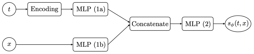
D.2 Neural network and stochastic optimization
The architecture of the neural networks we employed is illustrated in Fig. 5. For all numerical experiments, optimization was performed using the stochastic gradient algorithm of Kingma and Ba (2014) with a momentum of and learning rate of .
D.3 Ornstein–Uhlenbeck process
Let be an Ornstein–Uhlenbeck process, defined by (1) with linear drift function and identity diffusion coefficient . In this analytically tractable example, for any , the transition density of is a normal density , with the following mean and variance
Hence the logarithmic gradient term in the Doob’s -transform of (2) is
and the score of the transition density in (4) is
For this example, we can select the auxiliary process of Schauer et al. (2017) as the Ornstein–Uhlenbeck process by setting , in which case the linear guiding term is exact, and the Radon–Nikodym derivative in (34) satisfies .
For dimension and varying either the time horizon or the terminal state , we employed a time-discretization stepsize of , optimization iterations, and sample paths per iteration. For the case of and varying , we decreased the stepsize and increased the number of optimization iterations and the capacity of the neural network with dimension.
D.4 Interest rates model
We consider a special case of an interest rates model in Aït-Sahalia and Lo (1998), defined by (1) with drift function with and diffusion coefficient . This diffusion has a stable stationary point at , and its transition density is known and given by
for , where denotes the modified Bessel function of order . The logarithmic gradient term in the Doob’s -transform of (2) is
and the score of the transition density in (4) is
where denotes the derivative of .
Numerical experiments for all employed a time-discretization stepsize of , optimization iterations, sample paths per iteration with unique initial conditions sampled from the gamma distribution with shape and rate . We select the auxiliary process of Schauer et al. (2017) as an Ornstein–Uhlenbeck process with drift and unit diffusion coefficient. The choice of is based on the first-order Taylor approximation
D.5 Cell model
Our numerical experiments for all and employed a time-discretization stepsize of , optimization iterations, and sample paths per iteration. In our implementation of the guided proposal bridge, we choose an auxiliary Ornstein–Uhlenbeck process with drift function with and parameterized by a matrix whose columns are eigenvectors and a diagonal matrix whose diagonal entries are eigenvalues. This eigendecomposition facilities computation of matrix exponentials appearing in the expressions of the transition density and the gradient .
Following Schauer et al. (2017), we optimize the parameters by minimizing the Kullback–Leibler divergence , where denotes the law of the diffusion bridge and is the law induced by the guided proposal bridge process in (33). As considered in Schauer et al. (2017), we employ importance sampling to approximate the intractable objective by rewriting it as
| (35) |
where denotes expectation with respect to the proposal law with reference parameters that are obtained from earlier iterations of a stochastic gradient descent algorithm.
Initialization of is crucial as estimators of the gradient of (35) with respect to will have large variance when the importance sampling approximation under is poor. For this application, we initialize by setting , corresponding to starting with the identity matrix and choosing to induce mean-reversion towards the stable stationary point . After each gradient update, we also perform projection to ensure that columns of are orthogonal.