Simulating periodic systems on quantum computer
Abstract
The variational quantum eigensolver (VQE) is one of the most appealing quantum algorithms to simulate electronic structure properties of molecules on near-term noisy intermediate-scale quantum devices. In this work, we generalize the VQE algorithm for simulating periodic systems. However, the numerical study of an one-dimensional (1D) infinite hydrogen chain using existing VQE algorithms shows a remarkable deviation of the ground state energy with respect to the exact full configuration interaction (FCI) result. Here, we present two schemes to improve the accuracy of quantum simulations for periodic systems. The first one is a modified VQE algorithm, which introduces an unitary transformation of Hartree-Fock orbitals to avoid the complex Hamiltonian. The second one is a Post-VQE approach combining VQE with the quantum subspace expansion approach (VQE/QSE). Numerical benchmark calculations demonstrate that both of two schemes provide an accurate description of the potential energy curve of the 1D hydrogen chain. In addition, excited states computed with the VQE/QSE approach also agree very well with FCI results.
I Introduction
A well-defined, accurate and efficient electronic structure method is critical for interpreting material properties and for the prediction and designing of novel materials. Over years, a huge amount of effort has been devoted to systematically improve the computational accuracy for material simulations. Density functional theory (DFT) is a very powerful and elegant first principles method to explore ground-state properties of solids in materials science and condensed matter physics while the accuracy of DFT calculations strongly depends on exchange-correlation functional approximations CohMorYan08 ; ZhaTru08a ; CohMorYan12 . Recently, wave function based periodic electronic structure methods, such as second-order Møller-Plesset perturbation theory and coupled-cluster (CC) theory with single and double excitations (CCSD), have been successfully applied to problems in solids and low-dimensional nanomaterials SunBar96 ; AyaKudScu01 ; ShuDolFul99 ; GilAlfGir08 ; NolGilAlf09 ; BooGruKre13 ; McCSunCha17 ; HumTsaGru17 . Although wave function based methods offer a systematic approach for solving the many electron Schrödinger equation, their computational cost for accurately capturing strong electronic correlation effects is often prohibitive. For example, the exact full configuration interaction (FCI) method scales exponentially.
The recent advent of quantum computing provides a new pathway for solving many electron Schrödinger equation in polynomial time BraKit02 ; GeoAshNor14 ; Pre18 ; CaoRomOls19 ; McAEndAsp20 . With rapid progresses in quantum chemistry based quantum algorithms, experimental studies of molecular ground-state and excited-state properties have been extensively performed DuXuPen10 ; PerMcCSha14 ; WecHasTro15 ; MalBabKiv16 ; HarMon17 ; ReiWieSvo17 ; KanMezTem17 ; HemMaiRom18 ; SanWanGen18 ; GriEcoBar19 . For example, Du et al. reported a quantum phase estimation (QPE) simulation of the ground-state energy of the hydrogen molecule using NMR DuXuPen10 . Peruzzo et al. firstly proposed and realised the variational quantum eigensolver (VQE) algorithm on a photonic quantum processor for computing the ground-state energy of HeH+ PerMcCSha14 . Colless et al. used a superconducting-qubit-based processor to apply the quantum subspace expansion (QSE) approach to the H2 molecule, extracting both ground and excited states without the need for additional minimization ColRamDah18 .
The QPE AspDutLov05 and VQE algorithms PerMcCSha14 are two leading quantum algorithms for solving electronic structure problems on a quantum computer. The standard QPE algorithm evolves in time a quantum state under the Hamiltonian of interest, which offers an exponential speedup for determining the molecular spectra over classical methods. However, The practical implementation of QPE requires large, error-corrected quantum computer, which is believed to be out of reach in near-term quantum devices. On the other side, VQE provides an alternative quantum algorithm for near-term noisy intermediate-scale hardware because it requires a much shorter coherent time and can be implemented with massive parallelization MalBabKiv16 .
VQE applies the Rayleigh-Ritz variational principle to optimize the parameterized wave function, which finally minimizes the total energy functional. The variational optimization procedure is a hybrid quantum-classical algorithm, that is, the evaluation of various physical properties in terms of the expectation value of operators, such as the energy and gradient, is performed on the quantum computer and the update of parameters is performed on the classical computer WhiBiaAsp11 ; McCRomBab16 ; McCKimCar17 ; RomBabMcC18 ; ColRamDah18 . Given the wave function, the expectation value of operators is obtained by repeating the measurement many times and taking an average of measurement values. Integrated with the quantum computer, the state preparation and measurement of Pauli operators can be carried out in polynomial time. Therefore, it is possible to efficiently compute the energy or gradient on the quantum computer even when the wave function involves exponential configurations. Considering the superiority of VQE on near-term quantum devices, it has been widely used to solve various electronic structure problems CaoRomOls19 . However, the application of VQE to periodic systems is still lacking.
In this work, we generalize the VQE algorithm to periodic systems. The wave function ansatzes used in this work include the unitary coupled cluster (UCC) ansztz Eva11 ; PerMcCSha14 and the Adaptive Derivative-Assembled Pseudo-Trotter ansatz (ADAPT) recently proposed by Grimsley et al. GriEcoBar19 . With the periodic boundary condition, Hartree-Fock (HF) orbitals at sampling -points are defined in the complex number space in order to satisfy the translational symmetry. Given anti-Hermitian excitation operators used in UCC and ADAPT-VQE, coefficients of operators are assumed to be real in order to generate an unitary transformation. Therefore, the complex wave function variationally optimized in the real parameter space converges to a local minimum as discussed later in this work. In order to overcome this problem, we propose a modified VQE algorithm, named the VQE-K2G approach, which converts HF orbitals at sampling -points in an unit cell into real orbitals at -point in the corresponding supercell. After that, the wave function and Hamiltonian are also defined in the real space. Therefore, the VQE-K2G algorithm for periodic systems is expected to be as accurate as VQE for molecular systems. In addition, it is possible to improve the accuracy of VQE by combining it with QSE (VQE/QSE) SanWanGen18 , in which a reference state is prepared with VQE and the ground state wave function is obtained by diagonalizing the Hamiltonian sampled on the linear-response space of the reference state. VQE/QSE is expected to offer a good estimation of the exact wave function if VQE can prepare a reasonable reference state.
This paper is organized as follow. Section II gives a brief description of the theoretical methodology, covering periodic Hartree-Fock method, VQE algorithms with UCC and ADAPT ansatzes, the VQE algorithm for periodic systems and the VQE/QSE approach. In section III, we first compute the ground-state potential energy curve of an equispaced one-dimensional (1D) infinite hydrogen chain and analyze errors for different wave function ansatzes. We then assess the accuracy of two schemes, VQE-K2G and VQE/QSE, for ground-state calculations. Finally, we compute the potential energy curve of the first excited state for the 1D hydrogen chain with the VQE/QSE approach. A summary and outlook is given in Section IV.
II Theory
II.1 Periodic Hartree-Fock method
For the periodic system using atom-centered basis sets, Bloch atomic orbitals (BAO) are defined as
| (1) |
where is the translation vector and is a crystal momentum vector sampled in the unit cell. is the number of unit cells. HF orbitals at are expanded as a linear combination of BAOs,
| (2) |
which is also known as the Hartree-Fock-Roothaan approximation in first principles molecular calculations. Given HF orbitals, the corresponding one- and two-electron integrals can be computed VanKraMoh05 . The core electron potential is represented with the norm-conserving HGH pseudopotential KleByl82 ; GoeTetHut96 ; HarGoeHut98 , which removes the Coulomb singularity at the origin.
For each , the Hartree-Fock eigenvalue equation in the representation of BAOs is expressed as,
| (3) |
The Fock and overlap matrix elements are given by
| (4) |
Here is the kinetic energy, is the pseudopotential, is the Coulomb integral and is the exchange integral. In the real space, these matrices are given by
| (5) |
where indicates that the real space integration is performed in the unit cell. The density matrix can be obtained by averaging over sampling -points in an unit cell
| (6) |
where is the number of -points and is the number of occupied electrons.
II.2 VQE algorithm
In the VQE algorithm, one key ingredient is the wave function ansatz, which prepares an electronic state with a few parametrized unitary operators McCRomBab16 ,
| (7) |
where is the reference state. The parametrized wave function is optimized through Rayleigh-Ritz variational principle
| (8) |
The Hamiltonian in the second-quantized representation is expressed as
| (9) |
where is the one-electron integral, including kinetic energy and ionic potential (pseudopotential in this work) and is two-electron integral
| (10) |
The general one- and two-body excitation operators are defined as Noo00 ; MukKut04
| (11) |
and are the second-quantized creation and annihilation operators, satisfying the anticommutation relation.
II.2.1 Unitary coupled cluster ansatz
Unitary coupled cluster (UCC) ansatz is a common component in quantum variational algorithms Kut82 ; BarKucNog89 ; TauBar06 ; Eva11 ; HarShiScu18 . Different from the traditional CC (tCC) theory, the UCC energy and wave function are variationally determined according to Eq. (8). UCC wave function is defined as
| (12) |
A cluster operator for unitary CCSD (UCCSD) is expressed as TauBar06
| (13) |
Recently, a generalized UCCSD (UCCGSD) wave function has been introduced in the VQE algorithm Ron03 ; Maz04 ; Nak04 ; MukKut04 ; PerMcCSha14
| (14) |
Here indicate virtual orbitals; indicate occupied orbitals; and indicate general orbitals.
Although UCC is more robust than tCC, neither UCCSD or UCCGSD can be expanded using the Baker-Campbell-Hausdorff (BCH) formula at finite order. Therefore, an exact implementation of UCC on a classical computer scales exponentially. While the UCC wave function can be easily prepared on a quantum computer even if the reference state is a multiconfigurational state. Recently, the UCC ansatz has been widely used in experimental and theoretical chemistry simulations with the VQE algorithm PerMcCSha14 ; SheZhaZha17 .
At convergence, the stationary of the energy with respect to parameters is expressed as
| (15) |
where is the coefficient of anti-Hermitian operators for UCCGSD and for UCCSD. Recent numerical studies of small molecules with minimum basis sets demonstrate UCCGSD is far more robust and accurate than UCCSD LeeHugHea19 . The difference between UCCSD and UCCGSD is even more significant for periodic numerical simulations as shown later in this work.
On quantum computers, the implementation of UCC requires a decomposition of the exponentiated cluster operator into one- and two-qubit gates using an approximate scheme, such as the Trotter-Suzuki decomposition PouHasWec15 ; BabMcCWec15 ; GriClaEco20 ,
| (16) |
The UCC wave function with Trotterization is defined as
| (17) |
Therefore, the accuracy of UCC-VQE simulations strongly depends on the Trotter formula used, the number of Trotter steps, and the time-ordered sequence of operators in the UCC ansatz. In principle, the lower-order Trotter-Suzuki decomposition will result in larger error. However, given the wave function expression in Eq. (17) , the optimization of the wave function in the parameter space is able to cancel part of error and give a promising estimation of the ground-state energy.
II.2.2 ADAPT ansatz
Grimsley et al. recently proposed to approximate the exact wave function as an arbitrarily long product of general one- and two-body exponentiated operators GriEcoBar19 ,
| (18) |
In order to generate a maximally compact sequence of operators at convergence, the operator, , with the largest absolute pre-estimated gradient instead of all operators in the operator pool is used to update the wave function ansatz in the -th iteration. This indicates in Eq (18). The wave function is iteratively updated with
| (19) |
where is the reference state. The energy functional in the -th iteration is minimized by
| (20) |
The gradient of the energy functional with respect to parameters is formulated as
| (21) |
The convergence criteria is defined as
| (22) |
where is the pre-estimated gradient for the next iteration. For example, in the -th iteration, is defined with the wave function optimized in the -th iteration,
| (23) |
The variational optimization procedure for the ADAPT-VQE algorithm is summarized in Algorithm 1.
II.3 VQE algorithm for periodic systems
To extend VQE algorithms for periodic systems, we define the general one- and two-body operator pool with Bloch orbitals PieKowFan03 ; Dav03 ; Nak04 ,
| (24) |
where . The Hamiltonian is summed over sampling -points in an unit cell,
| (25) |
Because the Hamiltonian satisfies the translational symmetry based on the periodic boundary condition, general one- and two-body excitation operators must conserve crystal momentum,
| (26) |
where and are crystal momenta of creation operators and annihilation operators, respectively. is a reciprocal lattice vector. The primed summation in Eq. (25) indicates that one of the orbital momenta is fixed according to Eq. (26).
In order to analyze the difference between real and complex HF orbitals, we firstly introduce the contracted Schrödinger equation (CSE), which can be derived by contraction of the Schrödinger equation onto the space of two particles
| (27) |
The anti-Hermitian CSE (ACSE) is expressed as
| (28) |
which is also known as the Brillouin condition Maz06 ; Maz07 . The ACSE can be written as a sum of the real part (ACSE-Re)
| (29) |
and the imaginary part (ACSE-Im)
| (30) |
Therefore, for the real wave function, the variationally optimized ADAPT-VQE wave function is exactly the solution of ACSE. This agrees with the conclusion that ACSE enforce stationary of the energy with respect to a sequence of unitary transformation of the reference state. As the Bloch wave function is introduced, Eq. 29 is still satisfied according to the convergence criteria in Eq. 22 while the residual error of ACSE-Im that results in the deviation of the energy is not minimized in the variational optimization procedure. In order to remove the residual error of ACSE-Im, we transform HF orbitals at sampling -points in an unit cell into orbitals at -point in the corresponding supercell. This generates a set of real wave function and Hamiltonian for the VQE algorithm. A brief introduction of this scheme, named K2G, is described as following. HF orbitals in Eq. 2 can be rewritten as
| (31) |
where
| (32) |
and is the -th atomic orbital in -th ”replica”. The Fock matrix with the supercell atomic orbital basis is expressed as
| (33) |
Diagonalizing the Fock matrix, we obtain the real HF orbitals expanded with the supercell atomic basis functions.
| R | HF | UCCSD-VQE | UCCGSD-VQE | ADAPT(3) | |||||||
|---|---|---|---|---|---|---|---|---|---|---|---|
| ACSE-Re | ACSE-Im | ACSE-Re | ACSE-Im | ACSE-Re | ACSE-Im | ACSE-Re | ACSE-Im | ||||
| 0.5 | 19.23 | 4.82 | 18.69 | 5.03 | 0.02 | 8.28 | 0.02 | 8.21 | |||
| 0.6 | 16.64 | 4.66 | 16.01 | 5.08 | 0.03 | 7.11 | 0.02 | 7.12 | |||
| 0.7 | 14.86 | 4.78 | 14.10 | 5.46 | 0.03 | 6.39 | 0.02 | 6.38 | |||
| 0.8 | 13.61 | 4.89 | 12.71 | 5.67 | 0.02 | 5.89 | 0.03 | 5.89 | |||
| 0.9 | 12.70 | 4.99 | 11.66 | 5.86 | 0.02 | 5.58 | 0.06 | 5.60 | |||
| 1.0 | 12.04 | 5.07 | 10.92 | 6.04 | 0.03 | 5.35 | 0.04 | 5.38 | |||
| 1.1 | 11.56 | 5.14 | 10.97 | 6.25 | 0.03 | 5.15 | 0.09 | 5.21 | |||
| 1.2 | 11.21 | 5.20 | 11.06 | 6.45 | 0.03 | 4.96 | 0.05 | 4.99 | |||
| 1.3 | 10.96 | 5.25 | 11.16 | 6.65 | 0.03 | 4.76 | 0.06 | 4.79 | |||
| 1.4 | 10.80 | 5.28 | 11.23 | 6.85 | 0.05 | 4.62 | 0.05 | 4.63 | |||
| 1.5 | 10.67 | 5.32 | 11.22 | 7.05 | 0.05 | 4.44 | 0.05 | 4.44 | |||
| 1.6 | 10.65 | 5.33 | 11.07 | 7.25 | 0.09 | 4.30 | 0.07 | 4.30 | |||
| 1.7 | 10.81 | 5.35 | 10.72 | 7.45 | 0.14 | 4.10 | 0.05 | 4.14 | |||
| 1.8 | 11.03 | 5.35 | 10.08 | 7.62 | 0.18 | 4.02 | 0.06 | 4.00 | |||
| 1.9 | 11.24 | 5.34 | 9.14 | 7.73 | 0.25 | 3.85 | 0.08 | 3.83 | |||
| 2.0 | 11.47 | 5.33 | 7.93 | 8.35 | 0.13 | 3.50 | 0.04 | 3.82 | |||
| mMARE | 12.47 | 5.13 | 11.79 | 6.55 | 0.09 | 5.16 | 0.05 | 5.17 | |||
II.4 Quantum subspace expansion
The quantum subspace expansion approach has experimentally and theoretically proven to be one of the most useful techniques on near-term noisy intermediate-scale quantum devices McCKimCar17 ; ColRamDah18 ; SanWanGen18 ; PauAbhChu19 . In the original implementation of QSE, the reference state is prepared with the UCCSD ansatz and excited states are obtained by diagonalizing the Hamiltonian sampled on the linear response space with single excitations McCKimCar17 . It is straightforward to include higher-order excitation operators in QSE but at the expense of a sharp increase of measurements.
Given a set of linear-response excitation operators, , the configuration state space is defined as
| (34) |
The QSE wave function can be expressed as a linear combination of configuration state functions
| (35) |
The energy and wave function of the ground and excited states can be obtained by solving a generalized eigenvalue problem in the configuration state space
| (36) |
with eigenvectors , and a diagonal matrix of eigenvalues . The Hamiltonian matrix elements projected onto the configuration state space are given by
| (37) |
The overlap matrix elements are given by
| (38) |
which is required because the configuration states are not necessarily orthogonal to each other.
The QSE approach is kind of inspired by the linear response method. In order to accurately describe the target state, either a well-defined reference state or the inclusion of high-order excitations is necessary to obtain a converged result. The inclusion of high-order excitations indicates a polynomially increasing computational cost, which is prohibitive in medium- and large-size calculations. The VQE algorithm, especially ADAPT-VQE, is able to efficiently generate a reasonable reference state to approximate the target state even starting from a single-configurational Hartree-Fock state. Here, we combine VQE with the QSE approach by truncating excitation operators up to second order and apply it to study the ground state and excited states.
III Results
All calculations are performed with the modified ADAPT-VQE code ADAPT-VQE , which uses OpenFermion openfermion for mapping fermion operators onto qubit operators and PYSCF pyscf for all one- and two-electron integrals. The energy and wave function are optimized with the Broyden-Fletcher-Goldfarb-Shannon (BFGS) algorithm implemented in SciPy scipy . Gradients are computed with the finite difference approach for UCC-VQE and the analytical approach in Eq. (21) for ADAPT-VQE. All UCC-VQE calculations are performed without Trotterization, that is, Eq. (12) is used in our classical numerical simulations. All full configuration interaction results used for benchmark are obtained through explicitly diagonalizing the Hamiltonian in Hilbert space of qubits. The operator pool is composed of the spin-adapted operators in order to avoid the spin contamination. SVZ basis set together with GTH pseudopotential is used for all calculations.
Hereafter, for simplicity, we use ADAPT(m) to indicate an ADAPT-VQE calculation with = defined in Eq. (22). The prefix indicates a calculation with HF orbitals at -point in the supercell. For example, -ADAPT(m) indicates an ADAPT(m) calculation using the K2G scheme. ADAPT-SD and QSE-SD indicate that only one- and two-body excitations from occupied orbitals to virtual orbitals are involved in ADAPT and QSE, respectively. As stated in Eq. (18), we can specify in ADAPT-VQE calculations. In this work, we update the wave function with 30 operators identified with the largest absolute pre-estimated gradients in each iteration.
An 1D hydrogen chain with each hydrogen atom equispaced along a line is an interesting model system to explore elemental physical phenomena in modern condensed matter physics, such as an antiferromagnetic Mott phase and an insulator-to-metal transition MarClaFen19 . It also bridges the gap between the simply Hubbard model and realistic bulk materials. Depending on different electronic spin alignments, the hydrogen chain can be paramagnetic, antiferromagnetic or ferromagnetic phase. In this work, we place two hydrogen atoms in an unit cell, which is the minimum model system used to study the magnetic properties. Here, we benchmark the VQE algorithm for this 1D hydrogen chain model with one- and two-electron integrals obtained from a closed-shell Hartree-Fock calculation, which generates a paramagnetic state. We vary the hydrogen-hydrogen bond length, (H-H), and compute the potential energy curve of the hydrogen chain with various wave function ansatzes. In addition, we notice that a larger basis set and -points sampling are required to accurately describe periodic system. However, the performance of various wave function ansatzes are assessed with respect to the FCI result computed with the same basis set and -points. This will be not significantly affected by the accuracy of the theoretical method. In the following, all calculations are performed with -points, in which four -points are sampled along the hydrogen chain and one -point is sampled along other two orthogonal directions. In the VQE-K2G approach, the corresponding supercell atomic basis functions are obtained by including eight hydrogen atoms in this supercell.
III.1 Accuracy of VQE algorithms
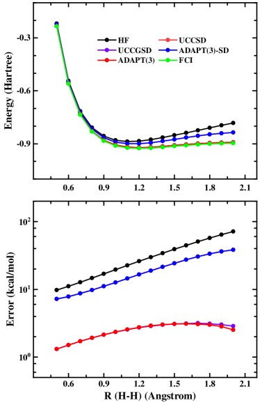
In Figure 1, we study the ground-state potential energy curve and the absolute energy error with HF, UCCSD-VQE, UCCGSD-VQE, ADAPT(3)-SD, ADAPT(3) and FCI by varying (H-H). HF fails to reproduce the exact energy curve with the mean error (ME) of 32.37 kcal/mol because the correlation effect totally misses in HF. UCCSD-VQE performs much better than HF with ME of 20.0 kcal/mol, but still significantly deviates from the exact FCI result. UCCSD is able to treat most weakly correlated systems while it suffers from the well-known problem of describing the strong electronic correlation effect. For example, as (H-H) increases from 0.5 to 2.0 Å, the absolute energy error of UCCSD-VQE increase from 7.19 to 38.16 kcal/mol. Note that the error of UCCSD-VQE in calculations of the 1D hydrogen chain is much larger than those in molecular calculations. For example, the largest absolute energy error is only 9.19 kcal/mol in calculations of a challenging system N2 with the STO-3G basis set LeeHugHea19 . ADAPT-SD shares the same operator pool with UCCSD. Here, ADAPT(3)-SD produces almost exactly the same result as UCCSD-VQE with the comparable ME of 19.87 kcal/mol. However, it should be kept in mind that ADAPT-SD and UCCSD are two different wave function ansatzes as discussed later.
UCCGSD-VQE gives a more promising ground state potential curve with the ME of only 1.58 kcal/mol. This agrees with the conclusion revealed in the previous study that the UCCGSD ansatz is far more robust and accurate than the simple UCCSD ansatz LeeHugHea19 . Analogous to ADAPT(3)-SD and UCCSD-VQE, ADAPT(3) and UCCGSD-VQE also share the same operator pool and give quite close results. However, ADAPT-VQE requires much fewer parameters to achieve the accuracy of UCCGSD-VQE. This is mainly because ADAPT-VQE approximates the exact wave function with a compact sequence of unitary transformation acting on the reference state. For example, the number of parameters in UCCGSD-VQE is fixed to be 236 while ADAPT(3) requires at most 144 parameters with (H-H) varying from 0.5 to 2.0 Å. This is achieved at the cost of computing pre-estimated gradients in Eq. (23).
In addition, for ADAPT(3), the absolute energy error of the 1D hydrogen chain is 2-3 magnitude larger than those of small molecules (LiH, BeH2 and H6) presented in Ref. GriEcoBar19, . As discussed in Section II.3, these large deviations of the energy results from the complex wave function and Hamiltonian used in the VQE algorithm. In order to analyze errors in detail, Table 1 shows the maximum absolute residual error (MARE) of ACSE-Re and ACSE-Im for HF, UCCSD-VQE, UCCGSD-VQE and ADAPT(3). MAREs of ACSE-Im in UCCGSD-VQE and ADAPT(3) are very close to those in HF and UCCSD-VQE while MEs of the energy in UCCGSD-VQE and ADAPT(3) are much smaller than those in HF and UCCSD-VQE. This reveals that a majority of the absolute energy error in HF and UCCSD-VQE originates from larger residual errors of ACSE-Re. In UCCGSD-VQE and ADAPT(3), the variational algorithm efficiently minimizes the MARE of ACSE-Re (0.1 kcal/mol) while it is not able to simultaneously minimize the MARE of ACSE-Im, which is left to be as large as 5.2 kcal/mol. Therefore, the error of UCCGSD-VQE and ADAPT(3) are largely attributed to the MARE of ACSE-Im. In order to improve the accuracy of the quantum variational algorithm for periodic systems, it is necessary to remove the residual error of ACSE-Im.
| HF | UCCSD-VQE | UCCGSD-VQE | ADAPT(3)-SD | ADAPT(1) | |
| ME | 32.73 | 20.00 | 2.53 | 19.87 | 3.94 |
| ADAPT(2) | ADAPT(3) | -UCCSD-VQE | -ADAPT(3)-SD | -ADAPT(X)-SD | |
| ME | 2.63 | 2.94 | 1.69 | 1.20 | 0.07 |
| -ADAPT(3) | ADAPT(3)-SD/QSE-SD | ADAPT(3)-SD/QSE | ADAPT(1)/QSE | ADAPT(2)/QSE | |
| ME | 0.05 | 3.75 | 1.30 | 0.00 | 0.00 |
III.2 VQE-K2G approach
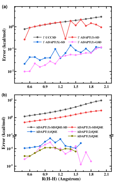
In Figure 2(a), we show the absolute energy error of various VQE-K2G approaches as a function of (H-H), which systematically remove the residual error of ACSE-Im through an unitary transformation of HF orbitals at sampling -points. Analogous to molecular simulations, the potential energy curve computed with -ADAPT(3) agrees quite well with the exact curve since the variationally optimized wave function strictly satisfies ACSE with the norm of residual errors less than . ADAPT-VQE is an adaptive algorithm and the wave function ansatz is self-consistently grown. Therefore, when the potential energy curve is scanned, the energy discontinuity may appear if the convergence thresh is not small enough. For example, errors in the absolute energy computed with -ADAPT(3)-SD dramatically fluctuates as shown in Figure 2(a). Here, we also compute the energy with a tighter convergence thresh = in -ADAPT(m)-SD, named -ADAPT(X)-SD, for comparison. -ADAPT(X)-SD gives well converged results with ME of 0.07 kcal/mol, which is even comparable to ME of 0.05 kcal/mol in -ADAPT(3).
In comparison with UCCSD-VQE, -UCCSD-VQE gives a much better description of the potential energy curve of 1D hydrogen chain. The maximum deviation of the energy for -UCCSD-VQE at Å is only 2.75 kcal/mol. Different from what is shown in Figure 1, -ADAPT(3)-SD and -ADAPT(X)-SD give more accurate results than -UCCSD-VQE. In the ADAPT-VQE method, high-order excitations are ultimately included after a sequence of low-order exponentiated excitation operators acting on the wave function. A tighter convergence thresh implies that a larger in Eq. 18 is required to converge the wave function ansatz. As increases, the ADAPT-VQE wave function is in principle expanded in a larger configuration state space, which will improve the accuracy of the wave function ansatz. Therefore, the absolute energy error of -ADAPT(m)-SD is reduced as increases. This is very similar with the -UpCCGSD approach, in which a larger was often used to improve the accuracy LeeHugHea19 . UCCSD truncates excitation operators up to the second order and its wave function is optimized in a fixed parameter space. The inclusion of higher-order excitation operators is the most straightforward way to improve the accuracy of -UCCSD while at a steeply increasing computational cost.
It is worthy to mention that the accuracy of ADAPT(m)-SD can not be improved by increasing . The main reason is the limitation of crystal momenta conservation in excitation operators when HF orbitals at sampling k-points are used. Given excitation operators in Eq. (24), it is impossible to decompose these high-order excitations into the product of low-order excitation operators with crystal momentum conservation. For example, a quadruple excitation operator,
| (39) |
conserves crystal momentum
| (40) |
Eq. 26 is only sufficient but not necessary condition of Eq. (40). Therefore, ADAPT(m)-SD optimizes the wave function in a limited subspace of configuration states, which can not be simply overcome by increasing . Analogous to UCCSD, the explicit inclusion of higher-order excitations is necessary to improve the accuracy of ADAPT-SD.
III.3 Quantum subspace expansion
The quantum expansion subspace method is an alternative approach to improve the estimation of the energy over the reference state. Here, VQE/QSE can be considered as a Post-VQE method to improve the VQE algorithm. In Figure 2(b), we present the absolute energy error of the VQE/QSE approach as a function of (H-H). Here, the reference states are prepared with ADAPT(3)-SD, ADAPT(1), ADAPT(2) and ADAPT(3). The Hamiltonian matrix elements are sampled in the linear-response space of the VQE wave function with single and double excitations. All energy curves computed with ADAPT(m)/QSE exactly reproduce the FCI result with errors less than kcal/mol. This demonstrates that ADAPT(m) is able to obtain a quite reasonable reference state even with a very large convergence thresh, such as =. Although the mean error of 1.30 kcal/mol in ADAPT(3)-SD/QSE gets slightly beyond the chemical accuracy, this is almost 3-4 magnitude larger than MEs of ADAPT(m)/QSE. Since the Hamiltonian matrix elements are sampled in the same linear-response space, the reference state prepared with ADAPT(3)-SD is even worst than ADAPT(1). While the number of parameters in both ADAPT(3)-SD and ADAPT(1) is 30. For QSE-SD, the Hamiltonian is sampled in a much smaller linear response space of dimension being 153 (625 for QSE). This leads to a remarkable deviation of the potential energy curve for ADAPT(3)-SD/QSE-SD with the ME of 3.75 kcal/mol. Therefore, the accuracy of the QSE approach strongly depend on the reference state and the truncation of excitation operators. Sometimes higher-order excitations should be included in order to obtain a converged result.
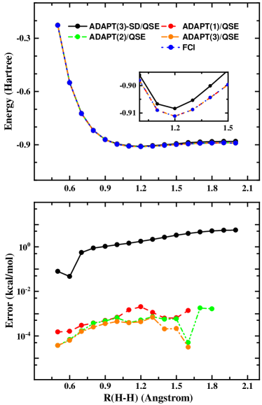
As the substantial success of the VQE algorithm in simulating ground-state properties, there is a broad interest in applying it to study excited states. For the 1D hydrogen chain, the potential energy surface of different electronic states is important to understand the rich and fascinating phase diagram in quantum material physics. In Figure 3, we present the first excited state energy and the absolute energy error of 1D hydrogen chain as a function of (H-H). The ground state wave function is obtained with ADAPT(m) or ADAPT(m)-SD and the first excited state is computed with the QSE approach. Regardless of the convergence thresh used in ground-state ADAPT(m) calculations, we obtain exactly the same curves as FCI. For ADAPT(m), mean errors of the first excited state energy are , , kcal/mol for =, = and =, respectively. The performance of ADAPT(3)-SD/QSE in excited-state calculations is quite similar with that in the ground state calculation. Although the absolute energy error of ADAPT(3)-SD/QSE is acceptable, we recommend to prepare the ground state with ADAPT(m) since it has been validated to be more robust and accurate.
IV Conclusion
In this work, we generalize the variational quantum eigenvalue algorithm for periodic systems. We first carry out classical VQE simulations of 1D infinite hydrogen chain with UCC and ADAPT ansatzes using HF orbitals at sampling -points. UCCSD-VQE and ADAPT(3)-SD totally fails to accurately describe the potential energy surface of 1D hydrogen chain. The absolute energy error of UCCGSD and ADAPT(3) is acceptable while it is at least 1-2 magnitude larger than that in the molecular simulation. The detailed analysis of residual error of ACSE reveals that the significant deviation of the energy results from the complex wave function and Hamiltonian generated based on HF orbitals at sampling -points.
Then, we present two schemes to overcome this problem in the VQE algorithm for periodic systems. One is the VQE-K2G approach, which avoids the complex wave function and Hamiltonian involved in VQE through an unitary transforming of HF orbitals at sampling -points in an unit cell into real orbitals at -point in a supercell. The VQE-K2G algorithm totally removes the residual error of imaginary part of ACSE and then achieve the same accuracy as the VQE algorithm in molecular simulations. Another scheme is the combination of VQE with the quantum subspace expansion approach, which offers a better estimation of the energy over the reference state. The VQE/QSE approach projects the Hamiltonian onto the linear response space of the reference state prepared with the VQE algorithm. This can be considered as a Post-VQE correction to the reference state energy. Numerical simulations demonstrates that both the VQE-K2G and VQE/QSE approaches provides an accurate enough description of the potential energy surface of 1D hydrogen chain. In addition, the accuracy of the VQE/QSE approach is 1-2 magnitude smaller than that of the VQE-K2G approach at the expense of steeply increasing measurements.
In this work, we come to the same conclusion that UCCGSD is more stable than UCCSD as stated in previous studies. The accuracy of UCCGSD without Trotterization is comparable to ADAPT. As Trotterization is introduced in UCC, the wave function expression of Eq. (17) is quite similar with that in ADAPT as shown in Eq. (18). However, UCCGSD uses the same coefficients of excitation operators in each Trotterization step while ADAPT uses difference coefficients. Therefore, ADAPT is expected to be more flexible than UCCGSD with Trotterization. In addition, ADAPT generates a optimized sequence of unitary transformation in Eq. (18), which is proven to be necessary to find the lowest energy GriClaEco20 . However, at the beginning of each iteration, ADAPT-VQE needs to compute the gradients in Eq. (21) at the expense of measurements where is the number of basis functions. Further work should be devoted to reduce the number of measurements.
Finally, we note that the wave function ansatz based on Gaussian basis functions offer a well established solution of electronic structure problems. While a large Gaussian basis set is often required to obtain the converged result. In order to accurately simulate electron structure properties in material science, an alternative approach is to use the Wannier basis function MarMosYat12 or adaptive local basis function in a discontinuous Galerkin framework ZhaLinHu17 , which can reach the complete basis set limit with much fewer basis functions.
V Acknowledgments
This work is supported by the National Natural Science Foundation of China (21688102,21825302,21803065), by National Key Research and Development Program of China (2016YFA0200604), Anhui Initiative in Quantum Information Technologies (AHY090400).
References
- (1) Cohen, A. J.; Mori-Sanchez, P.; Yang, W. Science 2008, 321, 792–794.
- (2) Zhao, Y.; Truhlar, D. G. Acc. Chem. Res. 2008, 41, 157–167.
- (3) Cohen, A. J.; Mori-Sanchez, P.; Yang, W. Chem. Rev. 2012, 112, 289–320.
- (4) Sun, J.; Bartlett, R. J. J. Chem. Phys. 1996, 104, 8553–8565.
- (5) Ayala, P. Y.; Kudin, K. N.; Scuseria, G. E. J. Chem. Phys. 2001, 115, 9698–9707.
- (6) Shukla, A.; Dolg, M.; Fulde, P.; Stoll, H. Phys. Rev. B: Condens. Matter Mater. Phys. 1999, 60, 5211–5216.
- (7) Gillan, M. J.; Alfẽ, D.; Gironcoli, S. d.; Manby, F. R. J. Comput. Chem. 2008, 29, 2098–2106.
- (8) Nolan, S. J.; Gillan, M. J.; Alfẽ, D.; Allan, N. L.; Manby, F. R. Phys. Rev. B: Condens. Matter Mater. Phys. 2009, 80, 165109.
- (9) Booth, G. H.; Grüneis, A.; Kresse, G.; Alavi, A. Nature 2013, 493, 365–370.
- (10) McClain, J.; Sun, Q.; Chan, G. K.-L.; Berkelbach, T. C. Journal of Chemical Theory and Computation 2017, 13, 1209-1218.
- (11) Hummel, F.; Tsatsoulis, T.; Grüneis, A. The Journal of Chemical Physics 2017, 146, 124105.
- (12) Bravyi, S. B.; Kitaev, A. Y. Ann. Phys. 2002, 298, 210–226.
- (13) Georgescu, I. M.; Ashhab, S.; Nori, F. Rev. Mod. Phys. 2014, 86, 153–185.
- (14) Preskill, J. Quantum 2018, 2, 79.
- (15) Cao, Y.; Romero, J.; Olson, J. P.; Degroote, M.; Johnson, P. D.; Kieferová, M.; Kivlichan, I. D.; Menke, T.; Peropadre, B.; Sawaya, N. P. D.; Sim, S.; Veis, L.; Aspuru-Guzik, A. Chemical Reviews 2019, 119, 10856–10915.
- (16) McArdle, S.; Endo, S.; Aspuru-Guzik, A.; Benjamin, S. C.; Yuan, X. Rev. Mod. Phys. 2020, 92, 015003.
- (17) Du, J.; Xu, N.; Peng, X.; Wang, P.; Wu, S.; Lu, D. Phys. Rev. Lett. 2010, 104, 030502.
- (18) Peruzzo, A.; McClean, J.; Shadbolt, P.; Yung, M.-H.; Zhou, X.-Q.; Love, P. J.; Aspuru-Guzik, A.; O’ Brien, J. L. Nat. Commun. 2014, 5, 4213.
- (19) Wecker, D.; Hastings, M. B.; Troyer, M. Phys. Rev. A: At., Mol., Opt. Phys. 2015, 92, 042303.
- (20) O’ Malley, P. J. J. et al. Phys. Rev. X 2016, 6, 031007.
- (21) Harrow, A. W.; Montanaro, A. Nature 2017, 549, 203.
- (22) Reiher, M.; Wiebe, N.; Svore, K. M.; Wecker, D.; Troyer, M. Proc. Natl. Acad. Sci. U. S. A. 2017, 114, 7555.
- (23) Kandala, A.; Mezzacapo, A.; Temme, K.; Takita, M.; Brink, M.; Chow, J. M.; Gambetta, J. M. Nature 2017, 549, 242.
- (24) Hempel, C.; Maier, C.; Romero, J.; McClean, J.; Monz, T.; Shen, H.; Jurcevic, P.; Lanyon, B. P.; Love, P.; Babbush, R.; Aspuru-Guzik, A.; Blatt, R.; Roos, C. F. Phys. Rev. X 2018, 8, 031022.
- (25) Santagati, R.; Wang, J.; Gentile, A. A.; Paesani, S.; Wiebe, N.; McClean, J. R.; MorleyShort, S.; Shadbolt, P. J.; Bonneau, D.; Silverstone, J. W.; Tew, D. P.; Zhou, X.; O’ Brien, J. L.; Thompson, M. G. Sci. Adv. 2018, 4, eaap9646.
- (26) Grimsley, H. R.; Economou, S. E.; Barnes, E.; Mayhall, N. J. Nat. Commun. 2019, 10, 3007.
- (27) Colless, J. I.; Ramasesh, V. V.; Dahlen, D.; Blok, M. S.; Kimchi-Schwartz, M. E.; McClean, J. R.; Carter, J.; de Jong, W. A.; Siddiqi, I. Phys. Rev. X 2018, 8, 011021.
- (28) Aspuru-Guzik, A.; Dutoi, A. D.; Love, P. J.; Head-Gordon, M. Science 2005, 309, 1704.
- (29) Whitfield, J. D.; Biamonte, J.; Aspuru-Guzik, A. Mol. Phys. 2011, 109, 735–750.
- (30) McClean, J. R.; Romero, J.; Babbush, R.; Aspuru-Guzik, A. New J. Phys. 2016, 18, 023023.
- (31) McClean, J. R.; Kimchi-Schwartz, M. E.; Carter, J.; de Jong, W. A. Phys. Rev. A: At., Mol., Opt. Phys. 2017, 95, 042308.
- (32) Romero, J.; Babbush, R.; McClean, J. R.; Hempel, C.; Love, P. J.; Aspuru-Guzik, A. Quantum Sci. Technol. 2018, 4, 014008.
- (33) Evangelista, F. A. J. Chem. Phys. 2011, 134, 224102.
- (34) VandeVondele, J.; Krack, M.; Mohamed, F.; Parrinello, M.; Chassaing, T.; Hutter, J. Comput. Phys. Commun. 2005, 167, 103.
- (35) Kleinman, L.; Bylander, D. M. Phys. Rev. Lett. 1982, 48, 1425–1428.
- (36) Goedecker, S.; Teter, M.; Hutter, J. Phys. Rev. B: Condens. Matter Mater. Phys. 1996, 54, 1703.
- (37) Hartwigsen, C.; Goedecker, S.; Hutter, J. Phys. Rev. B: Condens. Matter Mater. Phys. 1998, 58, 3641.
- (38) Nooijen, M. Phys. Rev. Lett. 2000, 84, 2108.
- (39) Mukherjee, D.; Kutzelnigg, W. Chem. Phys. Lett. 2004, 397, 174.
- (40) Kutzelnigg, W. J. Chem. Phys. 1982, 77, 3081.
- (41) Bartlett, R. J.; Kucharski, S. A.; Noga, J. Chem. Phys. Lett. 1989, 155, 133.
- (42) Taube, A. G.; Bartlett, R. J. Int. J. Quantum Chem. 2006, 106, 3393.
- (43) Harsha, G.; Shiozaki, T.; Scuseria, G. E. J. Chem. Phys. 2018, 148, 044107.
- (44) Ronen, S. Phys. Rev. Lett. 2003, 91, 123002.
- (45) Mazziotti, D. A. Phys. Rev. A: At., Mol., Opt. Phys. 2004, 69, 012507.
- (46) Nakatsuji, H. Phys. Rev. Lett. 2004, 93, 030403.
- (47) Shen, Y.; Zhang, X.; Zhang, S.; Zhang, J.-N.; Yung, M.-H.; Kim, K. Phys. Rev. A: At., Mol., Opt. Phys. 2017, 95, 020501.
- (48) Lee, J.; Huggins, W. J.; Head-Gordon, M.; Whaley, K. B. J. Chem. Theory Comput. 2019, 15, 311–324.
- (49) Poulin, D.; Hastings, M. B.; Wecker, D.; Wiebe, N.; Doberty, A. C.; Troyer, M. Quantum Info. Comput. 2015, 15, 361.
- (50) Babbush, R.; McClean, J.; Wecker, D.; Aspuru-Guzik, A.; Wiebe, N. Phys. Rev. A 2015, 91, 022311.
- (51) Grimsley, H. R.; Claudino, D.; Economou, S. E.; Barnes, E.; Mayhall, N. J. J. Chem. Theory Comput. 2020, 16, 1–6.
- (52) Piecuch, P.; Kowalski, K.; Fan, P.-D.; Jedziniak, K. Phys. Rev. Lett. 2003, 90, 113001.
- (53) Davidson, E. R. Phys. Rev. Lett. 2003, 91, 123001.
- (54) Mazziotti, D. A. Acc. Chem. Res. 2006, 39, 207-215.
- (55) Mazziotti, D. A. Phys. Rev. A 2007, 75, 022505.
- (56) Ollitrault, P. J.; Kandala, A.; Chen, C.-F.; Barkoutsos, P. K.; Mezzacapo, A.; Pistoia, M.; Sheldon, S.; Woerner, S.; Gambetta, J.; Tavernelli, I. arXiv:quant-ph 2019, arXiv:1910.12890.
- (57) https://github.com/mayhallgroup/adapt-vqe
- (58) McClean, J. R. et al. arXiv:quant-ph 2017, arXiv:1710.07629.
- (59) Sun, Q.; Berkelbach, T. C.; Blunt, N. S.; Booth, G. H.; Guo, S.; Li, Z.; Liu, J.; McClain, J. D.; Sayfutyarova, E. R.; Sharma, S.; Wouters, S.; Chan, G. K.-L. Wiley Interdisciplinary Reviews: Computational Molecular Science 2018, 8, e1340.
- (60) Virtanen, P. et al. Nature Methods 2020, 17, 261–272.
- (61) Motta, M. et al. arXiv:cond-mat.str-el 2019, arXiv:1911.01618.
- (62) Marzari, N.; Mostofi, A. A.; Yates, J. R.; Souza, I.; Vanderbilt, D. Rev. Mod. Phys. 2012, 84, 1419–1475.
- (63) Zhang, G.; Lin, L.; Hu, W.; Yang, C.; Pask, J. E. J. Comput. Phys. 2017, 335, 426–443.