Simulation of Lindblad equations for quarkonium in the quark-gluon plasma

Let us start from a general remark on the regimes of open quantum systems [6, 36]. This is very important because the useful basis of open system depends on the regime. In the open quantum system, there are three important time scales: environmental correlation time ($\tau_{E}$), system relaxation time ($\tau_{R}$), and system proper timescale ($\tau_{S}$). To derive Markovian master equation when the system-environment coupling is weak, it is necessary to assume hierarchy of time scales.

If $\tau_{E}\ll\tau_{R},\tau_{S}$ is satisfied, the system in the quantum Brownian regime [48]. In this regime, the fast environmental modes couple to an almost “frozen” system. For example, if the system-environment coupling is given by $H_{\text{sys-env}}\sim X(t)x(t)$, where $X(t)$ and $x(t)$ are system and environmental operators, the system is perturbed by the environment approximately through $X(t)$, because the system evolution is slow $X(t-\tau_{E})\simeq X(t)-{\tau_{E}}\dot{X}(t)\simeq X(t)$¹¹1 We adopt the interaction picture for $H_{\text{sys-env}}$.. This approximation scheme is the derivative expansion, which is frequently used in many other fields.

If $\tau_{E},\tau_{S}\ll\tau_{R}$ is satisfied, the system is in the quantum optical regime. In this regime, the above approximation is not always possible²²2 It can be possible when $\tau_{E}\ll\tau_{S}\ll\tau_{R}$.. Instead, the system energy basis $|\epsilon\rangle$ provides a good description. In this basis, $X(t)=\sum e^{-i\omega t}X_{\epsilon,\epsilon^{\prime}}|\epsilon\rangle\langle\epsilon^{\prime}|$ contains rapid phases $\omega\equiv\epsilon^{\prime}-\epsilon$. If transition spectrum is discrete with $\Delta\omega=|\omega-\omega^{\prime}|\sim 1/\tau_{S}$, interference between transitions with different energy gaps $\omega\neq\omega^{\prime}$ is effectively lost at time scale of $\tau_{R}$ since $e^{-i\Delta\omega\tau_{R}}\sim e^{-i\tau_{R}/\tau_{S}}\sim 0$. This approximation scheme is called rotating wave approximation.

In the quantum Brownian regime, the density matrix with canonical variables $\langle X|\rho|X^{\prime}\rangle$ is reasonably convenient while in the quantum optical regime, the density matrix with eigenstate basis $\langle\epsilon|\rho|\epsilon^{\prime}\rangle$ is preferred. Below, we analyze the quantum Brownian motion of a heavy quark pair, whose master equation is solved in the position representation. Note that descriptions based on the bound state levels are inconvenient, if not impossible, because typical quantum states are superposition of many levels. The condition for quantum Brownian motion $\tau_{E}\ll\tau_{S},\tau_{R}$ in the case of quarkonium will be examined in the next section³³3 If $\tau_{E}\sim\tau_{S}\ll\tau_{R}$, one would expect that quarkonium is in the quantum optical regime. However, one cannot use the rotating wave approximation because the transition spectrum takes continuous values above the threshold $|\omega|>E_{b}$ and $\Delta\omega=0$. One needs to take a classical limit and to treat each of the quarkonium bound states as point-like molecules, by which coupled Boltzmann equations for quarkonium and heavy quarks are obtained [24, 36]. .

The dynamics of quarkonium in the QGP in the quantum Brownian regime is modeled by the following Lindblad equation

Here, $\rho(t)$ is the reduced density matrix for the relative motion of the quarkonium, which consists of color-singlet and octet internal states $\rho(t)=\rho_{s}|s\rangle\langle s|+\rho_{o}|o\rangle\langle o|$. The effect of quantum and thermal fluctuations of gluons is given in $\Delta H$ and dissipator part containing $C_{n}(\vec{k})\ (n=+,-,d,f)$. They are parameterized by two functions $U(r)$ and $\gamma(r)$ (or its Fourier transform $\gamma(k)$),

where $T$ is the temperature of QGP, and $M$ is the heavy quark kinetic mass. The temperature is assumed to be $T\ll M$ so that thermal pair-creation of heavy quarks can be neglected.

The Hamiltonian shift $\Delta H$ represents the real part of system self-energy caused by the coupling to the environment⁴⁴4 From the structure of the Lindblad equation (1), the self-energy is readily extracted as $\displaystyle\Delta H-\frac{i}{2}\sum_{n}\int\frac{d^{3}k}{(2\pi)^{3}}C_{n}^{\dagger}(\vec{k})C_{n}(\vec{k}).$ (3) Conversely, by examining the imaginary part of the self-energy diagrams, one can infer the physical process described by the Lindblad operators. . $U(r)$ is the potential term given by virtual exchange of environmental gluons⁵⁵5 In the Potential Non-Relativistic QCD (pNRQCD) effective theory, $U(r)$ is interpreted as a part of the system Hamiltonian because gluon with momentum $k\sim 1/r$ is already integrated out in the vacuum before coupling the system and the finite temperature environment. . The next term corrects the potential term, which is obtained in the limit of static heavy quark, by introducing the effect of heavy quark recoils. Similar term ($\propto\{\vec{p},\vec{x}\}/MT$) is also found in the Caldeira-Leggett model [48] for the quantum Brownian motion.

The Lindblad operators $C_{n}(\vec{k})$ describe scatterings with momentum transfer $\vec{k}$ in various color channels in the singlet $|s\rangle$ and the octet $|o\rangle$, taking place with rates such as $4\gamma(k)/3$ for $n=+$. The subscripts $d$ and $f$ indicate structure constants $d_{abc}$ and $f_{abc}$ of SU(3) algebra involved in a scattering process. Schematically, in one-gluon ($g^{*}$) exchange process, an octet quarkonium scatters into

where $a,b,c$ are the octet charges. Note that $|o\rangle$ above denotes the octet after projection while $|b\rangle$ and $|c\rangle$ are individual octet states. See [36] for more technical details. The operators $V_{n}(\vec{k})\simeq e^{i\vec{k}\cdot\vec{r}/2}\pm e^{-i\vec{k}\cdot\vec{r}/2}+\cdots$ describe heavy quark momentum shifts in a scattering⁶⁶6 Recall that $\vec{r}=\vec{r}_{Q}-\vec{r}_{Q_{c}}$ is the relative coordinate between the heavy quark pair. Then, a scattering $\vec{p}_{Q}\to\vec{p}_{Q}+\vec{k}$ shifts the relative momentum $\vec{p}=(\vec{p}_{Q}-\vec{p}_{Q_{c}})/2\to\vec{p}+\vec{k}/2$ and $\vec{p}_{Q_{c}}\to\vec{p}_{Q_{c}}+\vec{k}$ shifts $\vec{p}\to\vec{p}-\vec{k}/2$. The leading term $e^{i\vec{k}\cdot\vec{r}/2}\pm e^{-i\vec{k}\cdot\vec{r}/2}$ represents the superposition of these two scatterings with relative signs (or phases in general) depending on the color channels. , where the omitted terms take account of the heavy quark recoils. Their explicit forms are

The terms due to the heavy quark recoils $\propto 1/T$ are required by the fluctuation-dissipation relation of thermal correlation functions in the QGP and are responsible for directing the quarkonium system toward the equilibrium [21, 36, 45]. This Lindblad equation describes the decoherence phenomena and dissipation of quarkonium.

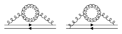
Original derivation [21, 36] was performed in the weak-coupling expansion $g\ll 1$ of Non-Relativistic QCD (NRQCD) and by assuming a particular configuration of heavy quark pair $r\sim 1/gT$. Self-energy diagrams considered in the derivation are shown in the Fig. 1. The three time scales are estimated as

Therefore, the condition $\tau_{E}\ll\tau_{R},\tau_{S}$ reads

The weak coupling assumption $g\ll 1$ is thus enough to justify the quantum Brownian motion. In this case, the dynamics of quarkonium is in the quantum Brownian regime and the functions $U(r)$ and $\gamma(k)$ are

Here $m_{D}=gT\sqrt{1+N_{f}/6}$ is the Debye screening mass for $N_{f}$ massless quark flavors. To be precise, the center-of-mass and relative dynamics are coupled and the former cannot be traced out. By projecting its full dynamics on the fixed center-of-mass momentum $\vec{P}=\vec{0}$, one gets the above Lindblad equation for the relative dynamics [27].

Although this Lindblad equation is obtained with a rather limited condition, there is a reason to believe that it captures essential features of quarkonium dynamics in the QGP. If the heavy quark pair distance is small, one can take a short distance extrapolation of (1) by a relatively mild assumption for the (non-)analyticity at the origin

to get (by replacing $\sum_{n}\int\frac{d^{3}k}{(2\pi)^{3}}$ with $\sum_{n}\sum_{j=x,y,z}$ in (1))

See [36] for more details. This Lindblad form is almost identical to that obtained from the pNRQCD effective field theory, which is based on the multi-pole expansion in terms of heavy quark pair distance [22, 23, 36]⁷⁷7 There is a minor technical difference. To get the Lindblad equation at $\mathcal{O}(r^{2})$, one needs to start from effective Lagrangian expanded up to $\mathcal{O}(r^{2})$. The Lindblad equation from pNRQCD is obtained from the Lagrangian up to $\mathcal{O}(r)$. .

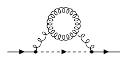
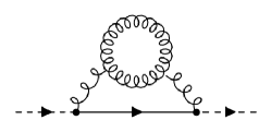
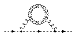
The derivation from pNRQCD does not need to assume the weak coupling $g\ll 1$ as long as the multi-pole expansion can be justified, i.e. $r\ll T^{-1},m_{D}^{-1}$. Self-energy diagrams considered in the derivation are shown in the Fig. 2. The three time scales in the non-perturbative region can be estimated by

For bottomonium, $M\approx 4.8{\rm GeV}$ and $4\alpha/3\sim 0.3-0.4$. Then, one of the conditions of quantum Brownian regime $\tau_{E}\ll\tau_{S}$ reads

which covers a large portion of temperature region available in the heavy-ion collisions, roughly $0.1{\rm GeV}\lesssim T\lesssim 0.5{\rm GeV}$. The other one $\tau_{E}\ll\tau_{R}$ is safely satisfied for bottom quarks in the heavy-ion collisions. In the Lindblad equations from pNRQCD, the coefficients $U_{2}$ and $\gamma_{2}$ are replaced with physical quantities with gauge invariant and non-perturbative definitions. To be specific, $U_{2}$ and $\gamma_{2}$ are responsible for the quarkonium mass shift and width at finite temperature and $\frac{4}{3}\gamma_{2}$ is the heavy quark momentum diffusion constant.

In this way, we expect that functions $U(r)$ and $\gamma(r)$ do exist which are compatible with both the multi-pole expansion $r\ll T^{-1},m_{D}^{-1}$ and the weak-coupling expansion $g\ll 1$ in soft regime $r\sim 1/gT$.

In this paper, we show the results of numerical simulations of the Lindblad model (1) with

The functions and its parameters are borrowed from our previous work [28], which are motivated from various known results about the heavy quark complex potential.

• •

  $U(r)$ of (13) models the short-range Coulomb attraction and the long-range screening.

  • –

    $\frac{4}{3}\alpha=0.3$ is chosen from the Coulomb part of the Cornell potential [50, 51].

  • –

    $m_{D}=2T$ is obtained by substituting $g=2,N_{f}=0$ into its perturbative result.

• •

  $\gamma(r)$ of (13) models the essential behaviors of its perturbative result (Fourier transform of (8)), which is a monotonically decreasing function with typical length scale $1/m_{D}$, decaying to 0 at long distance $r\gg 1/m_{D}$.

  • –

    The relation $m_{D}=2\ell_{\rm corr}^{-1}$ is obtained by equating the full width half maximum of $\gamma(r)$ in (13) and that from (8).

  • –

    $\gamma_{0}=\gamma(r=0)$ is obtained by substituting $g=2$ into its perturbative result $g^{2}T/4\pi$.

Note that the short distance behavior of $U(r)$ in (13) takes the form of (9a) only up to $U_{0}$, but the difference is subleading in $r\to 0$.

The simulation is mostly done with $T=0.1M$, which is $T\approx 0.48{\rm GeV}$ for bottomonium. The simulation is performed by the Quantum State Diffusion (QSD) method [52], which gives an algorithm to sample random wave functions evolving according to the nonlinear stochastic Schrödinger equation. Its stochastic evolution equation can be written in terms of the Lindblad operators as summarized in the Appendix A. In our simulation, we sampled thousands of random wave functions. For specific forms of the QSD equations, see [53]. The numerical cost to evolve one sample increases with the square of the lattice points $\sim N_{x}^{2}$ because the number of the Lindblad operators is $\sim N_{x}$. On the contrary, the dipole approximation reduces the number of the Lindblad operators to $\mathcal{O}(1)$ and the numerical cost increases only linearly with $N_{x}$.

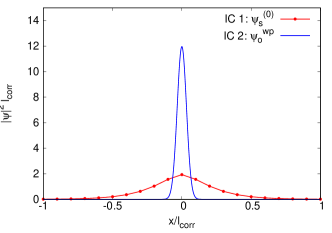
The system is prepared on a one-dimensional lattice with $N_{x}=255$ points with $\Delta x=1/M$ and the wave functions satisfy the periodic boundary condition. The origin $x=0$ is located at the center (the 128th lattice point) and the singular behavior of $U(r)\sim-\alpha/r$ is tamed by a cutoff $1/|x|\to 1/\sqrt{x^{2}+x_{c}^{2}}\equiv 1/|x|_{\rm reg}$ with $x_{c}=1/M$. Two different initial conditions (ICs) are adopted,

where $\psi_{s}^{(i)}\ (i=0,1,2,\cdots)$ denotes the singlet ground state ($i=0$) or an excited state ($i\geq 1$) in the screened potential (13). Note that only the ground state is bound in our screened potential in one dimension. The size of the wave packet $\psi_{o}^{\rm wp}(x)$ is $a=\frac{0.2}{\sqrt{2}}\cdot\frac{1}{(4/3)M\alpha}$. The wave functions are plotted in the Fig. 3. These initial conditions are motivated by two limiting scenarios for the initial conditions of the quarkonium in heavy-ion collisions — the bound state formation time is short enough (IC 1) and is too long (IC 2) compared to the initialization time. The IC 2 is similar to some of the initial conditions used in [54, 22, 23] and is based on the fact that the heavy quark pair production takes place locally by initial hard processes and mainly in the octet channel [55, 56].

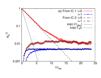
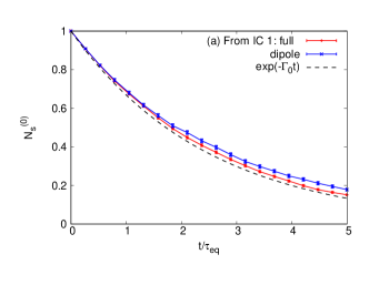
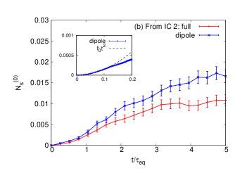
In Fig. 4(a), we show the evolution of state occupation numbers $N_{s}^{(i)}(t)\equiv\langle\psi_{s}^{(i)}|\rho(t)|\psi_{s}^{(i)}\rangle$ for $i=0,1$ starting from IC 1 and IC 2. Damping time due to friction $\tau_{\rm eq}\simeq 236/M$ and quantum decoherence time $\tau_{\rm dec}\simeq 191/M$ for the ground state will serve as useful reference scales. They are defined as

and computed at $T=0.1M$. For a wave function with macroscopic size, these time scales are hierarchical $\tau_{\rm eq}\gg\tau_{\rm dec}$. However, the bound state wave function $\psi_{s}^{(0)}(x)$ is localized with $\sqrt{\langle x^{2}\rangle}\simeq 2.67/M\ll 10/M=\ell_{\rm corr}$ and $\tau_{\rm eq}$ is not much different from $\tau_{\rm dec}$.

From the figure, one can observe that the relaxation of the excited singlet state takes place on the time scale of $\tau_{\rm eq}$ in both initial conditions. The relaxation takes place not only in the phase space but also in the color space. From IC 1, the singlet ground state first gets excited to the octet and then returns to the singlet. From IC 2, the initial state is already in the octet and thus the equilibration process is faster than from IC 1.

As for the singlet ground state, the relaxation from IC 2 takes place roughly in the time scale of $\tau_{\rm eq}$. However, the decay from IC 1 takes about 3 times longer than with $e^{-t/\tau_{\rm dec}}$. The reason is as follows. For bound states smaller than $\ell_{\rm corr}$, the decoherence is ineffective, and heavy quark recoils during the decoherence process are no longer subdominant. The recoil is responsible for irreversible processes such as friction in the classical limit, which prevents dissociation, and thus the decay process takes a longer time. Indeed, the damping $e^{-\Gamma_{0}t}$ with initial decay rate $\Gamma_{0}$ (defined later in Eq. (16)) including the recoil effect can quantitatively reproduce the numerical data before thermalization.

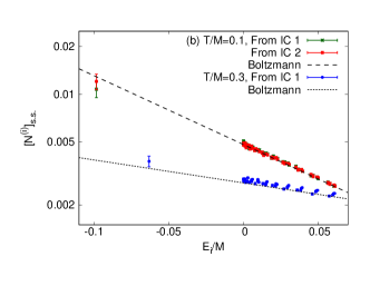
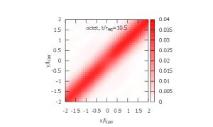
In Fig. 4(b), the distribution of eigenstates $[N^{(i)}]_{\rm s.s.}$ (both singlet and octet) in the steady state at $t\approx 24\tau_{\rm eq}$ is plotted for $T=0.1M$ and $0.3M$. Note that the occupation number of an octet eigenstate is defined as $N_{o}^{(i)}(t)\equiv\langle\psi_{o}^{(i)}|\rho(t)|\psi_{o}^{(i)}\rangle/8$. One can see that the distribution can be approximated well by the Boltzmann distribution with the environment temperatures, irrespective of the initial conditions for $T=0.1M$. The distributions are fitted by a two-parameter function $[N^{(i)}]_{\rm s.s.}=A^{\prime}\cdot e^{-E_{i}/T^{\prime}}$. The data for IC 1 and 2 with $T=0.1M$ are best fitted by $(A^{\prime},T^{\prime}/M)=(0.0049,0.0994)$ and $(0.0049,0.1012)$, respectively, and those for $T=0.3M$ are by $(0.0029,0.2846)$. The relative errors are $\lesssim 1\%$ except for the last one ($T^{\prime}/M=0.2846$ with a relative error $\sim 4\%$). Although the steady state solution of the Lindblad equation (1) is not known, the Lindblad operators approximately satisfy the detailed balance relation with the recoil terms and the equilibration to the Boltzmann distribution is expected.

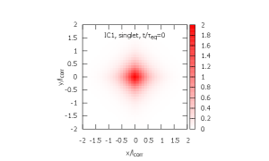
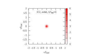
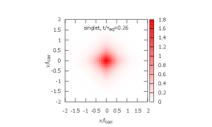
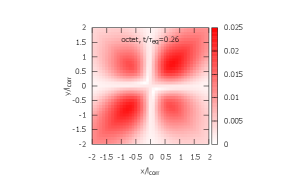
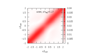
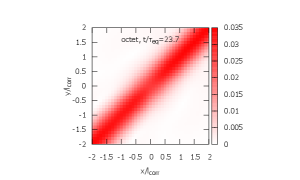
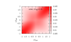
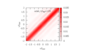
In Figs. 5, 6, and 7, time evolution of the density matrix is shown. The initial density matrices for ICs 1 and 2 are shown in Fig. 5. Both are localized at the origin $x\sim y\sim 0$ within $\lesssim\ell_{\rm corr}$. In Figs. 6 and 7, the top figures are the singlet density matrices and the bottom figures are the octet density matrices.

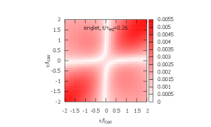
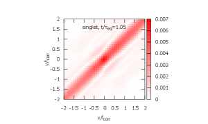
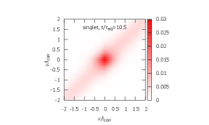
From IC 1, the evolution of the density matrix proceeds by the three steps.

1. (1)

   The singlet ground state is excited to octet as a color dipole. Note that the singlet-to-octet transition is forbidden at $xy=0$ in the recoilless limit (see Eq. (5)) [left; $t=0.26\tau_{\rm eq}$].

2. (2)

   The octet density matrix is diagonalized and gets close to its steady state. At this stage, the singlet density matrix is still dominated by the ground state and its time evolution is only visible in the magnitude at the origin [center; $t=5.27\tau_{\rm eq}$].

3. (3)

   De-excitation from the octet to the singlet is observed and the system finally reaches its steady state [right; $t=23.7\tau_{\rm eq}$].

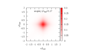
From IC 2, the evolution of the density matrix proceeds by the three steps.

1. (1)

   The octet wave packet expands rapidly and transitions to the singlet state with a wide distribution. Note that the octet-to-singlet transition is forbidden at $xy=0$ in the recoilless limit (see Eq. (5)) [left; $t=0.26\tau_{\rm eq}$].

2. (2)

   The singlet and octet density matrices are diagonalized. The octet density matrix is close to its steady state while the singlet density matrix is not because the magnitude at the origin is still small [center; $t=1.05\tau_{\rm eq}$].

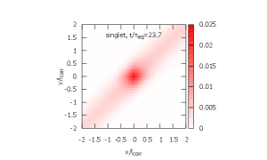
3. (3)

   The singlet density matrix now contains enough ground state occupation and the system finally reaches its steady state [right; $t=10.5\tau_{\rm eq}$].

From this simulation, we find that the quarkonium relative distribution extends far beyond the scale $\ell_{\rm corr}$ both for the singlet and the octet. Naively, one would expect that the dipole approximation does not work. In the next section, we examine this naive expectation and find that the dipole approximation actually works reasonably well as long as the ground state occupation $N_{s}^{(0)}(t)$ in the short time scale matters ($t\sim\mathcal{O}(\tau_{\rm eq})$).

In the relativistic heavy-ion collisions, the typical lifetime of the QGP fireball is $\tau_{\rm hic}\sim 10{\rm fm}\sim 250/M$ for bottom quark mass $M\approx 4.8{\rm GeV}$. This time scale is comparable to the equilibration time for bottom quarks $\tau_{\rm eq}\simeq 236/M$ at $T=0.1M$ and is shorter than $\tau_{\rm eq}$ at lower temperatures because $\tau_{\rm eq}\propto 1/T^{2}$. In such time scales, as we show below, the dipole approximation turns out to be applicable for the ground state occupation number $N_{s}^{(0)}(t)$. In Fig. 8, we compare the simulations of the Lindblad model (1) and its dipole limit (10) for $\gamma_{2}$ only ($U(r)$ is not approximated by the small $r$ expansion). Semi-quantitative agreement is found until $t=5\tau_{\rm eq}$ or longer from IC 1 (Fig. 8(a)) and for $t\lesssim 1.5\tau_{\rm eq}$ from IC 2 (Fig. 8(b)).

From IC 1, the initial ground state is excited to the octet by the Lindblad operator $C_{+}(k)$ or $C_{+}$. There are two effects that allow us to neglect the probability of returning back to the singlet ground state — (i) The octet pair repels each other and the wave function gets extended so that the spatial overlap to the ground state becomes smaller, and (ii) The probability of flipping octet to singlet is suppressed by $\sim 1/N_{c}^{2}=1/9$ at large $N_{c}$ compared to that into an octet [57, 30]. Therefore, the time evolution of $N_{s}^{(0)}(t)$ is mostly governed by the excitation process by $C_{+}(k)$, whose coupling to a small ground state is well approximated by $C_{+}$. To confirm this interpretation, we also compare the numerical results and the decay formula $N_{s}^{(0)}(t)=e^{-\Gamma_{0}t}$ with

which only takes into account the excitation process by $C_{+}$. The numerical value for $\Gamma_{0}\simeq 1.71\times 10^{-3}M$ is obtained for $T=0.1M$. The quantitative agreement strongly supports our interpretation. Furthermore, it also suggests that simulating the Schrödinger equation with the non-Hermitian effective Hamiltonian $H_{\rm eff}$

which is derived by (10), would be sufficient for the calculation of survival probabilities of singlet bound states. This is an extension of the simulation of the Schrödinger equation with complex potential [58, 59, 60] by including the subleading terms from the heavy quark recoil.

From IC 2, the octet wave packet feeds down to the singlet while evolving by the repulsive force and diffusion. In short times, the evolution of the octet wave packet can be accurately described even with the dipole approximation. This is the reason why the dipole approximation seems to work in this case even though the octet wave function expands rapidly. To get an analytic estimate for a very short time, we calculate by the following two-step approach. Since $C_{-}$ flips the parity of the wave function, the octet wave function must contain the parity odd component. First, the octet wave packet is disturbed by $C_{d}$, which flips the parity, and the parity odd $(P=-1)$ octet component increases linearly in time by $\rho_{o}(\Delta t)_{P=-1}\simeq\Delta tC_{d}\rho_{o}(0)C_{d}^{\dagger}$. Then, it is this component that yields the ground state probability after its feed down to the singlet by $C_{-}$. The occupation number $N_{s}^{(0)}(t)$ evolves with

and the short-time behavior is expected to be quadratic in time $N_{s}^{(0)}(t)=f_{0}t^{2}$ with $f_{0}=2.66\times 10^{-7}M^{2}$. The quantitative agreement is found only for a short time $t\lesssim 0.12\tau_{\rm eq}$, showing that the linear approximation $\rho_{o}(\Delta t)_{P=-1}\propto\Delta t$ is not valid anymore at longer times. Since the Schrödinger equation with (17) cannot describe the octet-to-singlet transitions and the analytical estimate of the transition rate as above has limited applicability, the dipole approximation is probably the only alternative method to solve the Lindblad equation for this kind of initial condition.

References

- Yagi et al. [2005] K. Yagi, T. Hatsuda, and Y. Miake, Quark-Gluon Plasma: From Big Bang to Little Bang (Cambridge, 2005).
- Bernhard et al. [2019] J. E. Bernhard, J. S. Moreland, and S. A. Bass, Bayesian estimation of the specific shear and bulk viscosity of quark–gluon plasma, Nature Phys. 15, 1113 (2019).
- Chatrchyan et al. [2011] S. Chatrchyan et al. (CMS), Indications of suppression of excited states in PbPb collisions at = 2.76 TeV, Phys. Rev. Lett. 107, 052302 (2011), arXiv:1105.4894 [nucl-ex] .
- Chatrchyan et al. [2012] S. Chatrchyan et al. (CMS), Observation of sequential Upsilon suppression in PbPb collisions, Phys. Rev. Lett. 109, 222301 (2012), arXiv:1208.2826 [nucl-ex] .
- Khachatryan et al. [2016] V. Khachatryan et al. (CMS), Suppression of , and production in PbPb collisions at = 2.76 TeV, Submitted to: Phys. Lett. B (2016), arXiv:1611.01510 [nucl-ex] .
- Breuer and Petruccione [2002] H. P. Breuer and F. Petruccione, The theory of open quantum systems (Oxford University Press, 2002).
- Rivas and Huelga [2012] A. Rivas and S. F. Huelga, Open quantum systems, Vol. 10 (Springer, 2012).
- Laine et al. [2007] M. Laine, O. Philipsen, P. Romatschke, and M. Tassler, Real-time static potential in hot QCD, JHEP 03, 054, arXiv:hep-ph/0611300 [hep-ph] .
- Beraudo et al. [2008] A. Beraudo, J. P. Blaizot, and C. Ratti, Real and imaginary-time Q anti-Q correlators in a thermal medium, Nucl. Phys. A806, 312 (2008), arXiv:0712.4394 [nucl-th] .
- Brambilla et al. [2008] N. Brambilla, J. Ghiglieri, A. Vairo, and P. Petreczky, Static quark-antiquark pairs at finite temperature, Phys. Rev. D78, 014017 (2008), arXiv:0804.0993 [hep-ph] .
- Rothkopf et al. [2012] A. Rothkopf, T. Hatsuda, and S. Sasaki, Complex Heavy-Quark Potential at Finite Temperature from Lattice QCD, Phys. Rev. Lett. 108, 162001 (2012), arXiv:1108.1579 [hep-lat] .
- Young and Dusling [2013] C. Young and K. Dusling, Quarkonium above deconfinement as an open quantum system, Phys. Rev. C87, 065206 (2013), arXiv:1001.0935 [nucl-th] .
- Borghini and Gombeaud [2011] N. Borghini and C. Gombeaud, Dynamical Evolution of Heavy Quarkonia in a Deconfined Medium, (2011), arXiv:1103.2945 [hep-ph] .
- Borghini and Gombeaud [2012] N. Borghini and C. Gombeaud, Heavy quarkonia in a medium as a quantum dissipative system: Master equation approach, Eur. Phys. J. C72, 2000 (2012), arXiv:1109.4271 [nucl-th] .
- Akamatsu and Rothkopf [2012] Y. Akamatsu and A. Rothkopf, Stochastic potential and quantum decoherence of heavy quarkonium in the quark-gluon plasma, Phys. Rev. D 85, 105011 (2012), arXiv:1110.1203 [hep-ph] .
- Blaizot et al. [2016] J.-P. Blaizot, D. De Boni, P. Faccioli, and G. Garberoglio, Heavy quark bound states in a quark-gluon plasma: Dissociation and recombination, Nucl. Phys. A946, 49 (2016), arXiv:1503.03857 [nucl-th] .
- Blaizot and Escobedo [2018a] J.-P. Blaizot and M. A. Escobedo, Quantum and classical dynamics of heavy quarks in a quark-gluon plasma, JHEP 06, 034, arXiv:1711.10812 [hep-ph] .
- Blaizot and Escobedo [2018b] J.-P. Blaizot and M. A. Escobedo, Approach to equilibrium of a quarkonium in a quark-gluon plasma, Phys. Rev. D 98, 074007 (2018b), arXiv:1803.07996 [hep-ph] .
- Lindblad [1976] G. Lindblad, On the Generators of Quantum Dynamical Semigroups, Commun. Math. Phys. 48, 119 (1976).
- Gorini et al. [1976] V. Gorini, A. Kossakowski, and E. C. G. Sudarshan, Completely Positive Dynamical Semigroups of N Level Systems, J. Math. Phys. 17, 821 (1976).
- Akamatsu [2015] Y. Akamatsu, Heavy quark master equations in the Lindblad form at high temperatures, Phys. Rev. D 91, 056002 (2015), arXiv:1403.5783 [hep-ph] .
- Brambilla et al. [2017] N. Brambilla, M. A. Escobedo, J. Soto, and A. Vairo, Quarkonium suppression in heavy-ion collisions: an open quantum system approach, Phys. Rev. D96, 034021 (2017), arXiv:1612.07248 [hep-ph] .
- Brambilla et al. [2018] N. Brambilla, M. A. Escobedo, J. Soto, and A. Vairo, Heavy quarkonium suppression in a fireball, Phys. Rev. D 97, 074009 (2018), arXiv:1711.04515 [hep-ph] .
- Yao and Mehen [2019] X. Yao and T. Mehen, Quarkonium in-medium transport equation derived from first principles, Phys. Rev. D 99, 096028 (2019), arXiv:1811.07027 [hep-ph] .
- Rothkopf [2014] A. Rothkopf, A first look at Bottomonium melting via a stochastic potential, JHEP 04, 085, arXiv:1312.3246 [hep-ph] .
- Kajimoto et al. [2018] S. Kajimoto, Y. Akamatsu, M. Asakawa, and A. Rothkopf, Dynamical dissociation of quarkonia by wave function decoherence, Phys. Rev. D 97, 014003 (2018), arXiv:1705.03365 [nucl-th] .
- Akamatsu et al. [2018] Y. Akamatsu, M. Asakawa, S. Kajimoto, and A. Rothkopf, Quantum dissipation of a heavy quark from a nonlinear stochastic Schrödinger equation, JHEP 07, 029, arXiv:1805.00167 [nucl-th] .
- Miura et al. [2020] T. Miura, Y. Akamatsu, M. Asakawa, and A. Rothkopf, Quantum Brownian motion of a heavy quark pair in the quark-gluon plasma, Phys. Rev. D 101, 034011 (2020), arXiv:1908.06293 [nucl-th] .
- Ålund et al. [2021] O. Ålund, Y. Akamatsu, F. Laurén, T. Miura, J. Nordström, and A. Rothkopf, Trace preserving quantum dynamics using a novel reparametrization-neutral summation-by-parts difference operator, J. Comput. Phys. 425, 109917 (2021), arXiv:2004.04406 [physics.comp-ph] .
- Akamatsu et al. [2022] Y. Akamatsu, M. Asakawa, and S. Kajimoto, Dynamics of in-medium quarkonia in SU(3) and SU(2) gauge theories, Phys. Rev. D 105, 054036 (2022), arXiv:2108.06921 [nucl-th] .
- Brambilla et al. [2021a] N. Brambilla, M. A. Escobedo, M. Strickland, A. Vairo, P. Vander Griend, and J. H. Weber, Bottomonium suppression in an open quantum system using the quantum trajectories method, JHEP 05, 136, arXiv:2012.01240 [hep-ph] .
- Brambilla et al. [2021b] N. Brambilla, M. A. Escobedo, M. Strickland, A. Vairo, P. V. Griend, and J. H. Weber, Bottomonium production in heavy-ion collisions using quantum trajectories: Differential observables and momentum anisotropy, (2021b), arXiv:2107.06222 [hep-ph] .
- Brambilla et al. [2022] N. Brambilla, M. A. Escobedo, A. Islam, M. Strickland, A. Tiwari, A. Vairo, and P. Vander Griend, Heavy quarkonium dynamics at next-to-leading order in the binding energy over temperature, (2022), arXiv:2205.10289 [hep-ph] .
- Sharma and Tiwari [2020] R. Sharma and A. Tiwari, Quantum evolution of quarkonia with correlated and uncorrelated noise, Phys. Rev. D 101, 074004 (2020), arXiv:1912.07036 [hep-ph] .
- Yao et al. [2021] X. Yao, W. Ke, Y. Xu, S. A. Bass, and B. Müller, Coupled Boltzmann Transport Equations of Heavy Quarks and Quarkonia in Quark-Gluon Plasma, JHEP 01, 046, arXiv:2004.06746 [hep-ph] .
- Akamatsu [2022] Y. Akamatsu, Quarkonium in quark–gluon plasma: Open quantum system approaches re-examined, Prog. Part. Nucl. Phys. 123, 103932 (2022), arXiv:2009.10559 [nucl-th] .
- Yao [2021] X. Yao, Open quantum systems for quarkonia, Int. J. Mod. Phys. A 36, 2130010 (2021), arXiv:2102.01736 [hep-ph] .
- Sharma [2021] R. Sharma, Quarkonium propagation in the quark–gluon plasma, Eur. Phys. J. ST 230, 697 (2021), arXiv:2101.04268 [hep-ph] .
- Zhao and Rapp [2011] X. Zhao and R. Rapp, Medium Modifications and Production of Charmonia at LHC, Nucl. Phys. A 859, 114 (2011), arXiv:1102.2194 [hep-ph] .
- Song et al. [2011] T. Song, K. C. Han, and C. M. Ko, Charmonium production in relativistic heavy-ion collisions, Phys. Rev. C 84, 034907 (2011), arXiv:1103.6197 [nucl-th] .
- Zhou et al. [2014] K. Zhou, N. Xu, Z. Xu, and P. Zhuang, Medium effects on charmonium production at ultrarelativistic energies available at the CERN Large Hadron Collider, Phys. Rev. C 89, 054911 (2014), arXiv:1401.5845 [nucl-th] .
- Du and Rapp [2022] X. Du and R. Rapp, Non-equilibrium charmonium regeneration in strongly coupled quark-gluon plasma, (2022), arXiv:2207.00065 [nucl-th] .
- Abelev et al. [2014] B. B. Abelev et al. (ALICE), Centrality, rapidity and transverse momentum dependence of suppression in Pb-Pb collisions at =2.76 TeV, Phys. Lett. B734, 314 (2014), arXiv:1311.0214 [nucl-ex] .
- Adam et al. [2017] J. Adam et al. (ALICE), J/ suppression at forward rapidity in Pb-Pb collisions at TeV, Phys. Lett. B766, 212 (2017), arXiv:1606.08197 [nucl-ex] .
- Akamatsu and Miura [2022] Y. Akamatsu and T. Miura, Nonequilibrium evolution of quarkonium in medium, EPJ Web Conf. 258, 01006 (2022), arXiv:2111.15402 [hep-ph] .
- Spohn [1977] H. Spohn, An algebraic condition for the approach to equilibrium of an open n-level system, Letters in Mathematical Physics 2, 33 (1977).
- Schirmer and Wang [2010] S. Schirmer and X. Wang, Stabilizing open quantum systems by markovian reservoir engineering, Physical Review A 81, 062306 (2010).
- Caldeira and Leggett [1983] A. O. Caldeira and A. J. Leggett, Path integral approach to quantum Brownian motion, Physica A 121, 587 (1983).
- Moore and Teaney [2005] G. D. Moore and D. Teaney, How much do heavy quarks thermalize in a heavy ion collision?, Phys. Rev. C 71, 064904 (2005), arXiv:hep-ph/0412346 .
- Bali [2001] G. S. Bali, QCD forces and heavy quark bound states, Phys. Rept. 343, 1 (2001), arXiv:hep-ph/0001312 .
- Alford and Strickland [2013] J. Alford and M. Strickland, Charmonia and Bottomonia in a Magnetic Field, Phys. Rev. D 88, 105017 (2013), arXiv:1309.3003 [hep-ph] .
- Gisin and Percival [1992] N. Gisin and I. C. Percival, The quantum-state diffusion model applied to open systems, Journal of Physics A: Mathematical and General 25, 5677 (1992).
- Miura [2021] T. Miura, Quantum dissipation of quarkonium in the quark-gluon plasma via Lindblad equation, Ph.D. thesis, Osaka University (2021).
- Casalderrey-Solana [2013] J. Casalderrey-Solana, Dynamical Quarkonia Suppression in a QGP-Brick, JHEP 03, 091, arXiv:1208.2602 [hep-ph] .
- Cho and Leibovich [1996a] P. L. Cho and A. K. Leibovich, Color octet quarkonia production, Phys. Rev. D 53, 150 (1996a), arXiv:hep-ph/9505329 .
- Cho and Leibovich [1996b] P. L. Cho and A. K. Leibovich, Color octet quarkonia production. 2., Phys. Rev. D 53, 6203 (1996b), arXiv:hep-ph/9511315 .
- Escobedo [2021] M. A. Escobedo, Medium evolution of a static quark-antiquark pair in the large limit, Phys. Rev. D 103, 034010 (2021), arXiv:2010.10424 [hep-ph] .
- Islam and Strickland [2020] A. Islam and M. Strickland, Bottomonium suppression and elliptic flow from real-time quantum evolution, Phys. Lett. B 811, 135949 (2020), arXiv:2007.10211 [hep-ph] .
- Katz et al. [2022] R. Katz, S. Delorme, and P.-B. Gossiaux, One-dimensional complex potentials for quarkonia in a quark-gluon plasma, (2022), arXiv:2205.05154 [hep-ph] .
- Dong et al. [2022] L. Dong, Y. Guo, A. Islam, A. Rothkopf, and M. Strickland, The complex heavy-quark potential in an anisotropic quark-gluon plasma – Statics and dynamics, (2022), arXiv:2205.10349 [hep-ph] .
- Plenio and Knight [1998] M. B. Plenio and P. L. Knight, The Quantum jump approach to dissipative dynamics in quantum optics, Rev. Mod. Phys. 70, 101 (1998), arXiv:quant-ph/9702007 .