Simulation of traffic flow at a signalised intersection
Abstract
We have developed a Nagel-Schreckenberg cellular automata model for describing of vehicular traffic flow at a single intersection. A set of traffic lights operating either in fixed-time or traffic adaptive scheme controls the traffic flow. Closed boundary condition is applied to the streets each of which conduct a uni-directional flow. Extensive Monte Carlo simulations are carried out to find the model characteristics. In particular, we investigate the dependence of the flows on the signalisation parameters.
pacs:
PACS numbers: 89.40.-a, 02.50.Ey, 05.40.-a, 05.65.+bI Introduction
Modelling the dynamics of vehicular traffic flow by cellular automata has constituted the subject of intensive research by statistical physics during the past years schadrev ; helbingrev ; kernerbook ; tgf05 . City traffic was an early simulation target for statistical physicists bml ; nagatani1 ; nagatani2 ; cuesta ; freund ; chopard ; tadaki ; torok ; chau ; cs ; brockfeld . Evidently the optimisation of traffic flow at a single intersection is a preliminary but crucial step to achieve the ultimate task of global optimisation in city networks chitur . Nagatani proposed the first model for simulation of two crossing streets nagatani3 . Subsequently, Ishibashi and Fukui developed similar models ishibashi1 ; ishibashi2 . Recently, physicists have notably attempted to simulate the traffic flow at intersections and other traffic designations such as roundabouts foolad1 ; krbalek ; foolad2 ; foolad3 ; foolad4 ; helbing1 ; helbing2 ; helbing3 ; ray ; chen ; wang ; huang ; najem ; foolad5 . In principle, the vehicular flow at the intersection of two roads can be controlled via two distinctive schemes. In the first scheme, the traffic is controlled without traffic lights foolad5 ; foolad6 . In the second scheme, signalised traffic lights control the flow. In Ref.foolad2 , we have modelled the traffic flow at a single intersection with open boundary conditions on streets. Dependence of waiting times on signalisation and inflow rates were investigated in details. Along this line of study, our objective in this paper is to study in some depth, the characteristics of traffic flow and its optimisation in a single intersection with closed boundary condition. We will compare our results to those obtained in our recent study of a nonsignalised intersection foolad5 . In order to capture the basic features of this problem, we have constructed a NS cellular automata model. This paper has the following layout. In section II, the model is introduced and formulated. In sections III and IV, the results of Monte Carlo simulations of each controlling scheme are exhibited. Concluding remarks and discussions ends the paper in section V.
II Description of the Problem
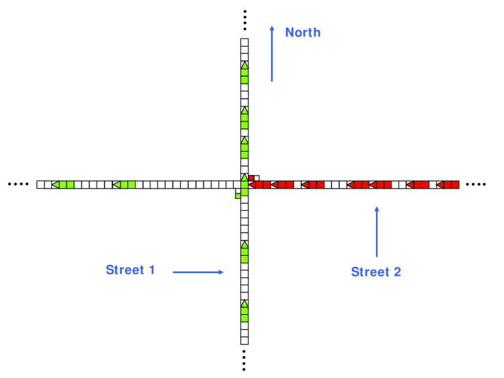
Imagine two perpendicular one dimensional closed chains each having sites. The chains represent urban roads accommodating unidirectional vehicular traffic flows. They intersect each other at the middle sites on the first and the second chain. With no loss of generality we take the flow direction in the first chain from south to north and in the second chain from east to west. (see Fig.1 for illustration). Cars are not allowed to turn. The discretisation of space is such that each car occupies an integer number of cells denoted by . The car position is denoted by the location of its head cell. Time elapses in discrete steps of and velocities take discrete values in which is the maximum velocity.
To be more specific, at each step of time, the system is characterized by the position and velocity configurations of cars. The system evolves under the Nagel-Schreckenberg (NS) dynamics ns . Let us now specify the physical values of our time and space units. The length of each car is taken 4.5 metres. Therefore, the spatial grid (cell length) equals to . We take the time step . Furthermore, we adopt a speed-limit of . The value of is so chosen to give the speed-limit value or equivalently . In this regard, is given by the integer part of . For instance, for , equals . In addition, each discrete increments of velocity signifies a value of which is also equivalent to the acceleration. For this gives the comfort acceleration . Moreover, we take the value of random breaking parameter at . A set of traffic lights controls the traffic flow. We discuss two types of signalisation in this paper: fixed-time and traffic responsive.
III Fixed Time Signalisation of lights
In this scheme the lights periodically turn into red and green. The period , hereafter referred to as cycle time, is divided into two phases. In the first phase with duration , the lights are green for the northward street and red for the westward one. In the second phase which lasts for timsteps the lights change their colour i.e.; they become red for the northward and green for the westward street. The gap of all cars are update with their leader vehicle except those two which are the nearest approaching cars to the intersection. These two cars need special attention. For these approaching cars gap should be adjusted with the signal in its red phase. In this case, the gap is defined as the number of cells right after the car’s head to the intersection point . If the head position of the approaching car lies in the crossing point the gap is zero. We note that at the time step when the traffic light goes red for a direction, portion of a car from that direction can occupy the crossing point. In this case the leading car of the queue in the other direction should wait until the passing car from the crossing point completely passes the intersection i.e.; its tail cell position become larger than . Now all the computational ingredients for simulation is at our disposal. The streets sizes are and we take . The system is update for time steps. After transients, two streets maintain steady-state currents denoted by and which are defined as the number of vehicles passing from a fixed location per time step. They are functions of global densities and and signal times and . We kept fixed in the second street and varied . Figure (2) exhibits the fundamental diagram of the first street i.e.; versus . The parameters are specified in the caption.
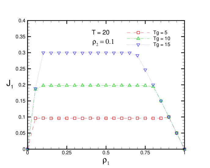
We observe that for each , linearly increase up to , then a lengthy plateau region is formed up to . If increases, becomes larger, becomes smaller, and the plateau height increases. This seems natural because by increasing the model tends to a normal NS model. The emergence of a plateau region is associated to defect-like role of the crossing point. The asymmetric simple exclusion process (ASEP), as a paradigm for non equilibrium processes in one dimension, with one defective site has been investigated within the Bethe Ansatz formalism in gunter93 and matrix product state hinrichsen97 . It is a well-established fact that a local defect can affect the low dimensional non-equilibrium systems on a global scale. This has been confirmed not only for ASEP lebowitz ; barma1 ; kolomeisky1 ; foolad6 but also for cellular automata models describing vehicular traffic flow chung ; yukawa . After the plateau, exhibits linear decrease versus in the same manner as in the fundamental diagram of a single road. Concerning the variation of cycle time , increasing the cycle time gives rise, on an equal basis, to increase both in the green and in the red portion of the cycle allocated to each street. The results show a notable increase in flows when is increased. This observation does not seem to comply to reality. The reason is due to unrealistic nature of NS rules. We now consider the flow properties in the second street. In Figure (3) we depict the behaviour of versus for various values of .
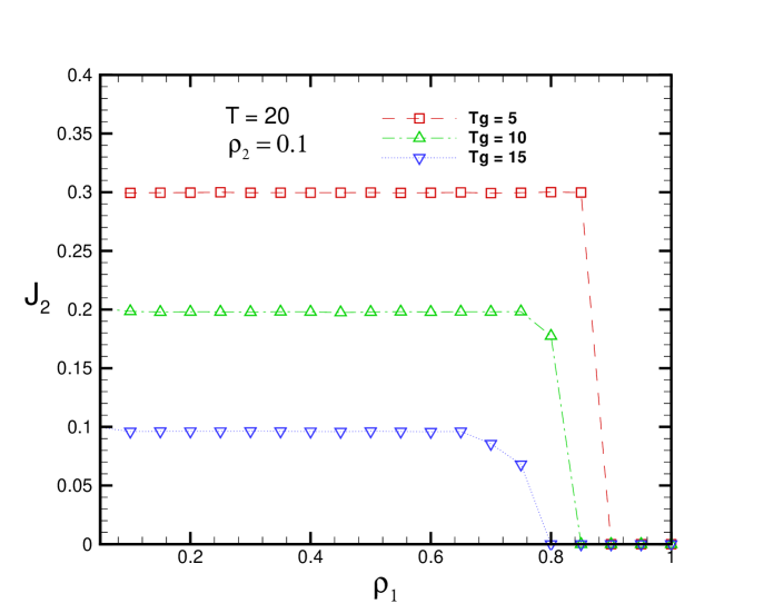
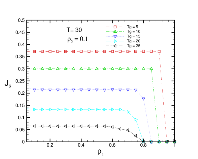
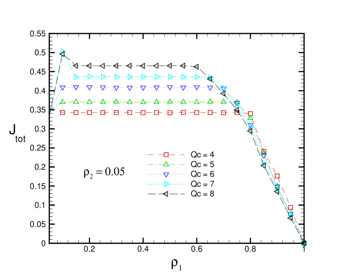
Although remains constant is affected by density variations in street . For each , as a function of exhibits two regimes. In the first regime, is almost independent of and remains constant up to . Afterwards in the second regime, exhibits a linearly decreasing behaviour towards zero. Analogous to , the existence of a wide plateau region indicates that street can maintain a constant flow capacity for a wide range of density variations in the first street. If is increased, the green time allocated to the second street decrease so we expect to exhibit a diminishing behaviour. This is in accordance to what figure (3) shows. In order to find a deeper insight, it would be illustrative to look at the behaviour of total current as a function of density in one of the streets. Evidently for optimisation of traffic one should maximize the total current therefore it is worth investigating how the total current behaves upon variation of the model parameters. Fig.(4) sketches this behaviour.
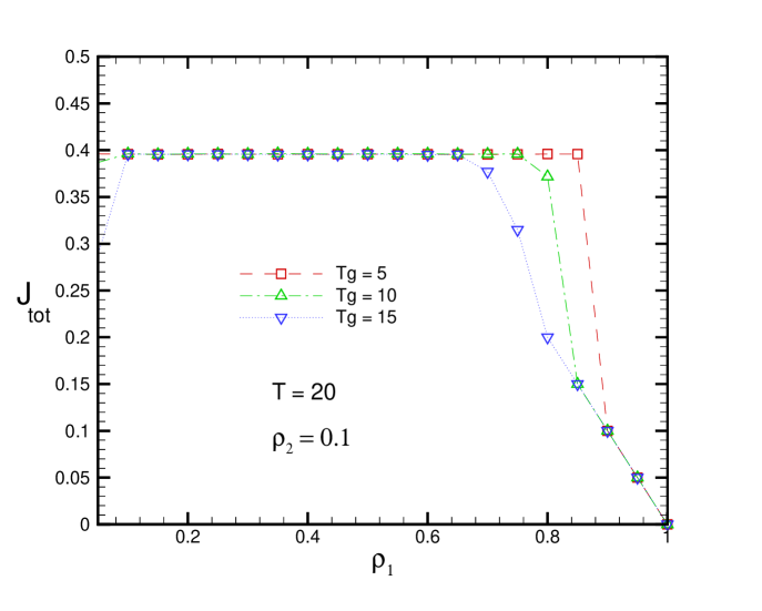
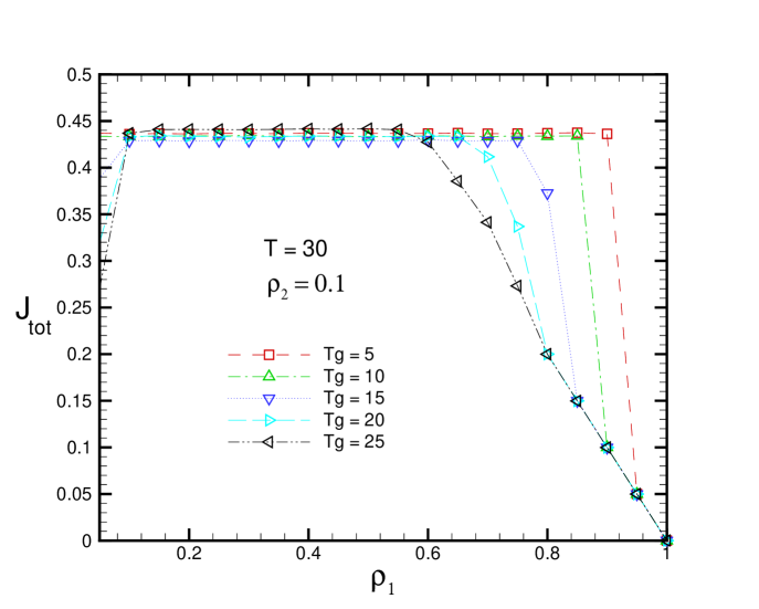
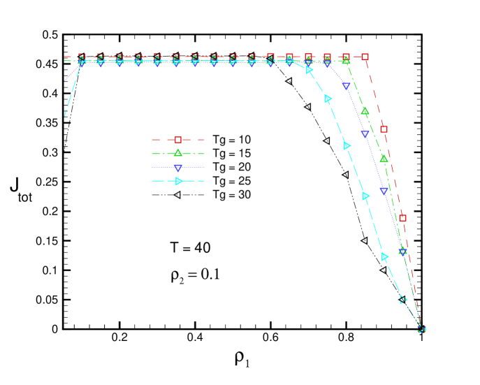
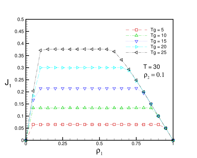
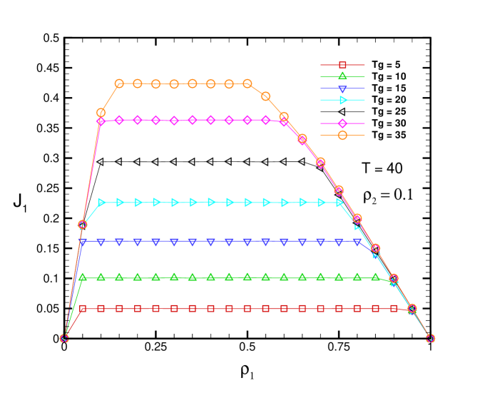
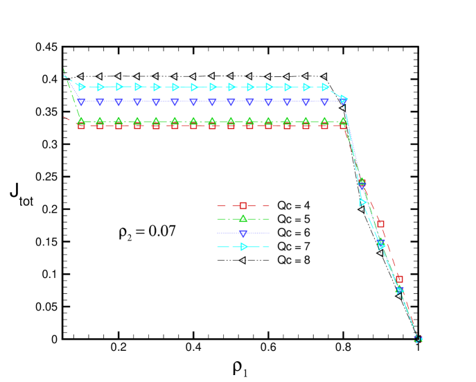
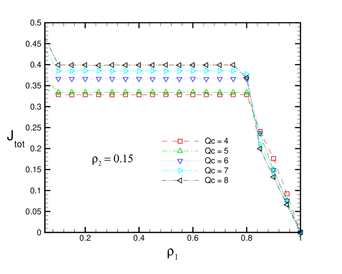
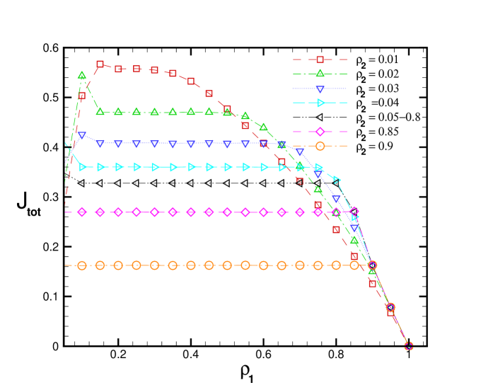
In general, the dependence of total current on depends on the value of . Except for small values of , total current increases with then it becomes saturated at a lengthy plateau before it starts its linear decrease. We have also examined the behaviour of for other values of . Figures (5) exhibits the results for and respectively.
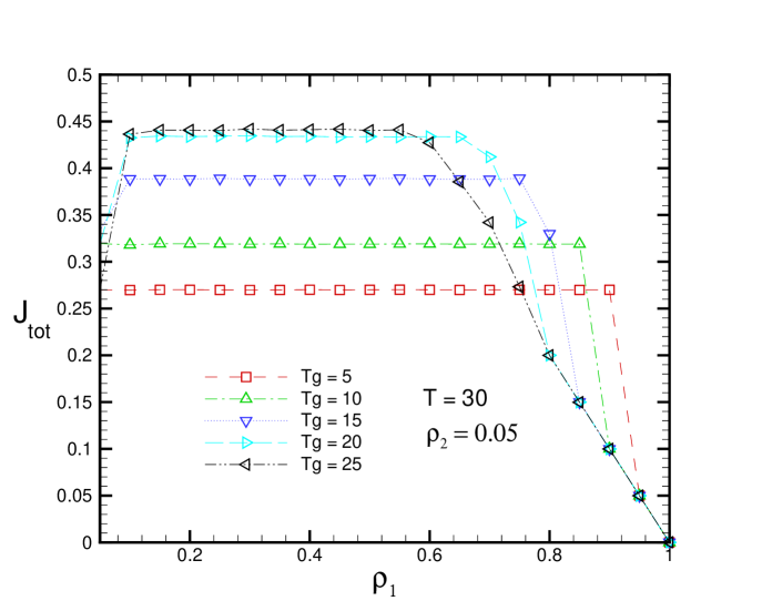
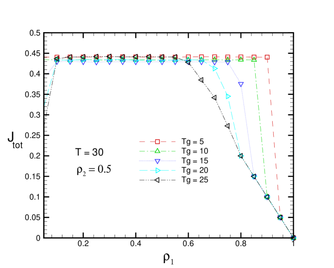
Our simulations confirm that for small up to total current shows a distinguishable dependence on in the entire range of especially in intermediate values. In contrast, for , we observe no significant dependence on in the intermediate but we observe notable dependence for large .
III.1 Density profile and Queue Formation
In this section we try to investigate, in brief, the characteristics of queues which are formed behind the crossing point in the course of the red periods. To this end, in the following set of figures we exhibit the profile of density in the vicinity of intersection. This will provide much insight into the problem. In figure (6) we have sketched such profiles for three values of green times .
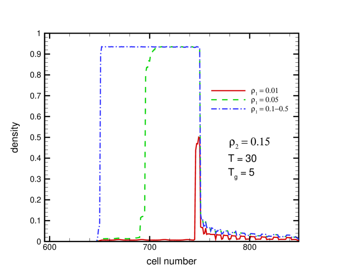
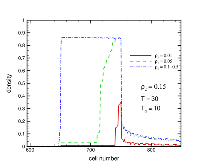
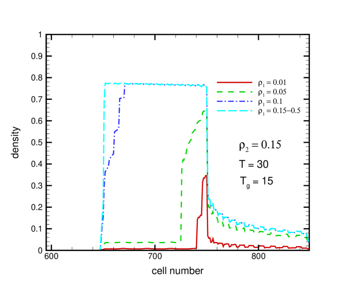
At each global density a high density region, hereafter referred to as HD, forms behind the crossing point. This corresponds to queue formation behind the crossing point. The length and height of this HD region grows with . Keeping constant, the length as well as the height of the HD region decreases with increasing . This is expected since by increasing the cars in the first street are given more time to pass the intersection and less cars will have to stop at red periods. Right after the crossing point, we observe a quick relaxation of the density profile to a low density region (hereafter referred to as LD). It would be natural to interpret the length of the HD region as the average queue length. We note that small oscillation in the profiles are not associated to inadequacy of simulation time. In fact their emergence is related to the updating rules of the NS model. Such oscillations have also been observed in the density-density correlation function in the NS model eisenblater .
IV Traffic Responsive Signalisation
In this section we present our simulations results for the so-called intelligent controlling scheme in which the traffic light cycle is no longer fixed webster ; bell . In this scheme which is some times called traffic responsive, the signalisation of traffic lights is simultaneously adapted to traffic status in the vicinity of intersection. This scheme has been implemented in simulation of traffic flow at intersections with open-boundary conditions foolad2 ; foolad4 . There exist numerous schemes in which traffic responsive signalisation can be prescribed. Three of these schemes are discussed in foolad2 . Here for brevity we discuss only one of these methods. To be precise, we define a cut-off queue length . The signal remain red for a street until the length of the corresponding queue formed behind the red light exceeds the cut-off length . At this moment the lights change colour. Apparently due to stochastic nature of cars movement, the cycle time will be subjected to variations and will no longer remain constant. In figure (7) we exhibit versus for various values of cut-off lengths and .
Analogous to fixed-time scheme, for given a lengthy plateau in forms. The plateau height as well as its length show a significant dependence on . higher are associated with smaller length and higher current. We have also examined larger values of . The results are qualitatively analogous the above graphs. The notable point is that for larger than 0.1, do not show a significant dependence on . Figure (8) depicts versus for .
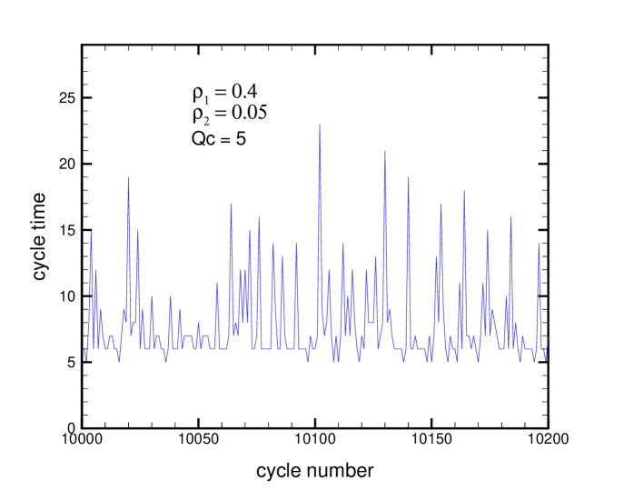
In figure (9) we have depicted the cycle lengths in the traffic responsive scheme which vary from cycle to cycle. The appearance of such behaviour remarks the adaptation of traffic lights in the responsive scheme.
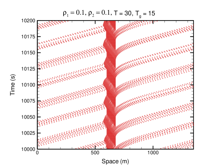
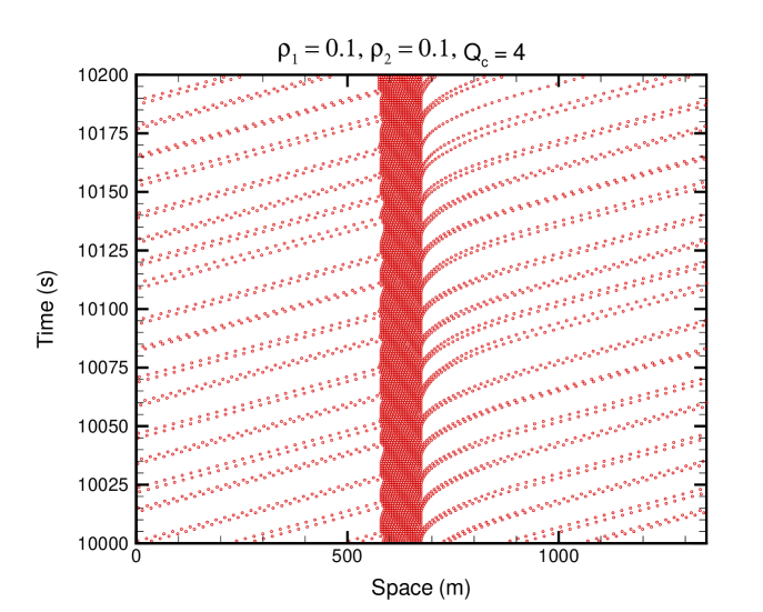
To shed some light onto the problem, we sketch space-time plots of vehicles. It is seen that in traffic responsive scheme, the cars spatial distribution is more homogeneous which is due to randomness in cycle times.
Lastly, we compare our results to those obtained in simulation of a nonsignalised intersection foolad5 . In a nonsignalised intersection, the cars yield to each other upon approaching the crossing point and the priority is give to the car which is closer to the crossing point. The total current versus in a nonsignalised intersection has the following form:
For larger than , the optimal current is roughly
in the nonsignalisation scheme whereas in the signalised
scheme with a fixed time strategy, the optimal value of
reaches beyond 0.45 (see Figs. 4 and 5) in a fixed time scheme and
0.4 in the traffic responsive scheme. It can be concluded that
signalisation strategies are apparently more efficient in comparison
to non-signalisation scheme.
V Summary and Concluding Remarks
By extensive Monte Carlo simulations, we have investigated the flow characteristics in a signalised intersection via developing a Nagel-Schreckenberg cellular automata model. We have considered two types of schemes: fixed-time and traffic responsive. In particular, we have obtained the fundamental diagrams in both streets and the dependence of total current on street densities. Our findings show hindrance of cars upon reaching the red light gives rise to formation of plateau regions in the fundamental diagrams. This is reminiscent of the conventional role of a single impurity in the one dimensional out of equilibrium systems. The existence of wide plateau region in the total system current shows the robustness of the controlling scheme to the density fluctuations. The overall throughput from the intersection shows a significant dependence on the cycle time in the fixed time scheme and on the queue cut-off length in the responsive scheme. Moreover, by plotting the density profiles, we have been able to quantify the characteristics of queues. Comparison to our previous results for a nonsignalised intersection shows the higher efficiency of the signalisation strategy. We remark that our approach is open to serious challenges. The lack of empirical data prevents us to judge how much our results are close to and to what degree they differ from reality. Our CA model allows for varying space and time grids. By their appropriate adjusting, we are able to reproduce a realistic acceleration. We emphasize that our model suffers from non realistic behaviour of car movement when the lights turn green. The crucial point is to model the braking and accelerating as realistic as possible. Empirical data are certainly required for this purpose. We expect the system characteristics undergo substantial changes if realistic yielding declaration is taken into account.
VI acknowledgement
We highly appreciate M. Abol Bashar for his fruitful helps and enlightening discussions.
References
- (1) D. Chowdhury, L. Santen and A. Schadschneider, Physics Reports, 329, 199 (2000).
- (2) D. Helbing, Rev. Mod. Phys., 73, 1067 (2001).
- (3) Physics of traffic flow, B. Kerner, Springer (2004).
- (4) R. Küne, A. Schadschneider, M. Schreckenberg and D.E. Wolf (eds.) Traffic and Granular flow 05, (Springer, 2007).
- (5) O. Biham, A. Middleton and D. Levine, Phys. Rev. A, 46, R6124 (1992).
- (6) T. Nagatani, J. Phys. Soc. Japan, 63, 1228 (1994); J. Phys. Soc. Japan, 64, 1421 (1995).
- (7) T. Nagatani, Phys. Rev. E, 51, 922 (1995); and T. Seno, Physica A, 207, 574 (1994).
- (8) J.A. Cuesta, F.C. Martines, J.M. Molera and A. Sanchez, Phys. Rev. E, 48, R4175 (1993).
- (9) J. Freund and T. Pöschel, Physica A, 219, 95 (1995).
- (10) B. Chopard, P.O. Luthi and P.A. Queloz J. Phys. A, 29, 2325 (1996).
- (11) S. Tadaki, Phys. Rev. E, 54, 2409 (1996); J. Physi. Soc. Jpn. 66, 514 (1997).
- (12) J. Török and J. Kertesz, Physica A, 231, 515 (1996).
- (13) H.F. Chau, K.Y. Wan and K.K. Yan, Physica A, 254, 117 (1998).
- (14) D. Chowdhury and A. Schadschneider, Phys. Rev. E, 59, R 1311 (1999).
- (15) E. Brockfeld, R. Barlovic, A. Schadschneider and and M. Schreckenberg, Phys. Rev. E, 64, 056132 (2001).
- (16) Y. Chitur and B. Piccoli, Discrete and Continuous Dynamical Systems B, 5, 599 (2005).
- (17) T. Nagatani, J. Phys. A, 26, 6625 (1993).
- (18) Y. Ishibash and M. Fukui, J. Phys. Soc. Japan, 65, 2793 (1996).
- (19) Y. Ishibash and M. Fukui, J. Phys. Soc. Japan, 70, 2793 (2001); J. Phys. Soc. Japan, 70, 3747 (2001).
- (20) M.E. Fouladvand and M. Nematollahi, Eur. Phys. J. B, 22, 395 (2001).
- (21) M. Krbalek and P. Sebra, J. Phys. A , 36, L7 (2003).
- (22) M. E. Fouladvand, Z. Sadjadi and M. R. Shaebani J. Phys. A: Math. Gen, 37, 561 (2004).
- (23) M. E. Fouladvand, Z. Sadjadi and M. R. Shaebani Phys. Rev. E, 70, 046132 (2004).
- (24) M. E. Fouladvand, M. R. Shaebani and Z. Sadjadi J. Phys. Soc. Japan, 73, No. 11, 3209 (2004).
- (25) D. Helbing, S. Lmmer and J.P. Lebacque, in C. Deissenberg and R.F. Hartl(eds.), Optimal Control and Dynamic Games, p. 239, Springer, Dortrecht, 2005; arXive physics/0511018.
- (26) S. Lmmer, H. Kori, K. Peters and D. Helbing, Physica A, 363, 39 (2006).
- (27) R. Jiang, D. Helbing, P. Kumar Shukla and Q-S Wu; Physica A, 368, issue 2, 567 (2006).
- (28) B. Ray and S.N. Bhattacharyya, Phys. Rev. E, 73, 036101 (2006).
- (29) R. X. Chen, K. Z. Bai and M. R. Liu, Chinese Physics, 15, Issue 7, 1471 (2006).
- (30) R. Wang, M. Liu, R. Kemp and M. Zhou, Int. J. Mod. Phys. C, 18, issue 5, 903 (2007).
- (31) D. W. Huang, Physica A, 383, Issue 2, 603 (2007).
- (32) M. Najem, Int. J. Mod. Phys. C, 18, Issue 6, 1047 (2007).
- (33) M. E. Foulaadvand and S. Belbasi, J. Phys. A: Math, Theor., 40, 8289 (2007).
- (34) M. E. Foulaadvand and M. Neek Amal, Euro. Phys. Lett., 80, issue 6, Article number 6002 (2007).
- (35) K. Nagel, M. Schreckenberg, J.Phys. I France, 2, 2221 (1992).
- (36) G. M. Schütz, J. Stat. Phys., 71, 471 (1993).
- (37) H. hinrichsen and S. Sandow J. Phys. A: Math. Gen, 30, 2745 (1997).
- (38) S. Janowsky and J. Lebowitz Phys. Rev. A, 45, 618 (1992).
- (39) G. Tripathy and M. Barma, Phys. Rev. Lett., 78, 3039 (1997).
- (40) A. B. Kolomeisky, J. Phys. A: Math, Gen., 31, 1153 (1998).
- (41) K.H. Chung and P.M. Hui, J. Phys. Soc. Jap., 63, 4338 (1994).
- (42) S. Yukawa, M. Kikuchi and S. Tadaki J. Phys. Soc. Jap., 63, 3609 (1994).
- (43) B. Eisenblätter, L. Santen, A. Schadschneider and M. Schreckenberg, Phys. Rev. E, 57, 1309 (1998).
- (44) F. Webster and B. Cobb in Traffic Signal Setting, (H.M.S Office, London, 1966).
- (45) M. G. Bell, Transp. Res. A, 26, No.4, 303 (1992).