Simulation study of estimating between-study variance and overall effect in meta-analysis of standardized mean difference
Abstract
Methods for random-effects meta-analysis require an estimate of the between-study variance, . The performance of estimators of (measured by bias and coverage) affects their usefulness in assessing heterogeneity of study-level effects, and also the performance of related estimators of the overall effect. For the effect measure standardized mean difference (SMD), we provide the results from extensive simulations on five point estimators of (the popular methods of DerSimonian-Laird, restricted maximum likelihood, and Mandel and Paule (MP); the less-familiar method of Jackson; the new method (KDB) based on the improved approximation to the distribution of the Q statistic by Kulinskaya, Dollinger and Bjørkestøl (2011) ), five interval estimators for (profile likelihood, Q-profile, Biggerstaff and Jackson, Jackson, and the new KDB method), six point estimators of the overall effect (the five related to the point estimators of and an estimator whose weights use only study-level sample sizes), and eight interval estimators for the overall effect (five based on the point estimators for ; the Hartung-Knapp-Sidik-Jonkman (HKSJ) interval; a modification of HKSJ; and an interval based on the sample-size-weighted estimator).
Keywords between-study variance, heterogeneity, random-effects model, meta-analysis, mean difference, standardized mean difference
1 Introduction
Meta-analysis is a statistical methodology for combining estimated effects from several studies in order to assess their heterogeneity and obtain an overall estimate. In this paper we focus on meta-analysis of standardized mean difference. The data and, often, existing tradition determine the choice of outcome measure. In a comparative study with continuous subject-level data for a treatment arm (T) and a control arm (C), the customary outcome measures are the mean difference (MD) and the standardized mean difference (SMD). The Cochrane Handbook (Higgins and Green, 2011, Part 2, Chapter 9) points out that the choice of MD over SMD depends on whether “outcome measurements in all studies are made on the same scale.” However, fields of application have established preferences: MD in medicine and SMD in social sciences.
If the studies can be assumed to have the same true effect, a meta-analysis uses a fixed-effect (FE) model (common-effect model) to combine the estimates. Otherwise, the studies’ true effects can depart from homogeneity in a variety of ways. Most commonly, a random-effects (RE) model regards those effects as a sample from a distribution and summarizes their heterogeneity via its variance, usually denoted by .The between-studies variance, , has a key role in estimates of the mean of the distribution of random effects; but it is also important as a quantitative indication of heterogeneity (Higgins et al., 2009). In studying estimation for meta-analysis of SMD, we focus first on and then proceed to the overall effect.
Veroniki et al. (2016) provide a comprehensive overview and recommendations on methods of estimating and its uncertainty. Their review, however, has two important limitations. First, the authors study only “methods that can be applied for any type of outcome data.” However, the performance of the methods that we study varies widely among effect measures. (Veroniki et al., 2016, Section 6.1) mention this only in passing as a hypothetical possibility. Second, any review on the topic, such as Veroniki et al. (2016), currently can draw on limited empirical information on the comparative performance of the methods. The (short) list of previous simulation studies for SMD is given in Table 1. From this table, it is clear that only three studies (Viechtbauer (2005) Petropoulou and Mavridis (2017) and Langan et al. (2018)) considered and compared several point estimators of .
However, to assess bias of the estimators of heterogeneity variance, Petropoulou and Mavridis (2017) use mean absolute error (the only performance measure reported for SMD in their Table S8), which is not a measure of bias; it is the linear counterpart of mean squared error.
Langan et al. (2018) studied bias and mean squared error of estimators of , as well as coverage of confidence intervals for the overall effect, but they used only one value of SMD=0.5 because they believed that the value of SMD does not matter. We show in our simulations that it does matter. Additionally, both Viechtbauer (2005) and Langan et al. (2018)) consider a very restricted range of values. There appear to be no studies at all on coverage of . Most of the simulation studies consider only inverse-variance-based estimation of the overall effect, and only two (Langan et al. (2018) and Hamman et al. (2018)) consider t-based confidence intervals for it.
Additionally, all moment-based point estimators of (i.e., the vast majority of the estimators listed in Table 1), use the inferior approximation to the distribution of Cochran’s statistic, which does not perform well for small to medium sample sizes (Kulinskaya et al., 2011).
To address this gap in information on methods of estimating the heterogeneity variance for SMD, we use simulation to study four methods recommended by Veroniki et al. (2016). These are the well-established methods of DerSimonian and Laird (1986), restricted maximum likelihood, and Mandel and Paule (1970), and the less-familiar method of Jackson (2013). We also include a new method based on improved approximations to the distribution of the statistic for SMD (Kulinskaya et al., 2011). We also study coverage of confidence intervals for achieved by five methods, including the Q-profile method of Viechtbauer (2007), a Q-profile method based on an improved approximation to the distribution of Cochran’s , and profile-likelihood-based intervals.
For each estimator of , we also study bias of the corresponding inverse-variance-weighted estimator of the overall effect. As our work progressed, it became clear that those inverse-variance-weighted estimators generally had unacceptable bias for SMD. Therefore, we added an estimator (SSW) whose weights depend only on the sample sizes of the Treatment and Control arms. We studied the coverage of the confidence intervals associated with the inverse-variance-weighted estimators, and also the HKSJ interval, the HKSJ interval using the improved estimator of , and the interval centered at SSW and using the improved in estimating its variance.
| Study | SMD measure | n and/or | K | Coverage of | Coverage of | ||||
| Viechtbauer 2005 | Hedges′s d | 0, 0.2 ,0.5 ,0.8 | 0, 0.01 ,0.025, 0.05 ,0.1 | 5, 10, 20, 40, 80 | DL | IV | |||
| ML | |||||||||
| REML | |||||||||
| HE | |||||||||
| HS | |||||||||
| Friedrich et al. 2008 | Hedges′s d | 0.2 ,0.5 ,0.8 | 0, 0.5 | 5, 10, 30 | DL | IV | IV | ||
| Petropoulou and Mavridis 2017 | 0 & 0.5 | 0,0.01,0.05,0.5 | 5,10,20, 30 | 20 | IV | IV | |||
| estimators | |||||||||
| of | |||||||||
| Langan et al. 2018 | Hedges′s d | 0.5 | depends on , 0%,15% | , | 2 ,3, 5, | REML | IV | IV | |
| 30%, 45%, 60%, | , , | 10, 20, 30, | CA | IV+t | |||||
| 75%, 90%, 95% | + | 50, 100 | PM or MP | IV +HKSJ | |||||
| HM | |||||||||
| SJ | |||||||||
| Lin 2018 | Cohen′s d | 0, 0.2, 0.5, 0.8, 1 | 0,0.2,0.5 | U(5,10), U(10,20), | 5, 10, 20, 50 | DL | IV | IV | |
| Hedges′s d | U(20,30), U(30,50) | ||||||||
| U(50,100), U(100,500), | |||||||||
| U(500,1000), | |||||||||
| Hamman et al. 2018 | Hedges′s d | 0,0.1,0.15,0.25 | 0,0.1,0.5,1, | 5,10,15,25,35, | REML | IV | IV +HKSJ | ||
| 0.35,0.5,0.6,0.75, | 2.5,5,10 | 14,16,20,25 | 45,55,75,100,125 | SSW(H) | |||||
| 1,1.25,1.5,2.5 | EW | ||||||||
| Marín-Martínez and | 0.2,0.5,0.8 | 0,0.04,0.08,0.16,0.32 | 5,10,20,40,100 | DL | FE | ||||
| Sánchez-Meca 2010 | ML | IV | |||||||
| HS |
Estimators of : DL - DerSimonian and Laird estimator, ML - Maximum likelihood, REML - Restricted maximum likelihood estimator, HE - Hedges estimator, HS - Hunter-Schmidt estimator, CA - Cochran ANOVA, PM or MP - Mandel-Paule estimator, - two-step Cochran ANOVA, -two-step DerSimonian-Laird, HM - Hartung-Makambi, SJ - Sidik-Jonkman, - alternative Sidik-Jonkman, BM - Bayes Modal estimator;
Estimators of : SSW(H) - sample-size-weighted (Hedges 1982), EW - equal weights, IV - inverse-variance-weighted, HS - Hunter and Schmidt (1990) total-sample-size-weighted;
Coverage of : IV - confidence interval centered at inverse-variance-weighted estimator of with z quantiles, IV+t - confidence interval centered at inverse-variance-weighted estimator of with t quantiles, IV+HKSJ - Hartung-Knapp-Sidik-Jonkman confidence interval centered at inverse-variance-weighted estimator of .
2 Study-level estimation of standardized mean difference
We assume that each of the studies in the meta-analysis consists of two arms, Treatment and Control, with sample sizes and . The total sample size in Study is . We denote the ratio of the control sample size to the total by . The subject-level data in each arm are assumed to be normally distributed with means and and variances and . The sample means are , and the sample variances are , for and or .
The standardized mean difference effect measure is
The plug-in estimator , known as Cohen’s , is biased in small samples, and we do not consider it further. Instead, we study the unbiased estimator
where , and the factor
often approximated by , corrects for bias (Hedges, 1983). This estimator of is sometimes called Hedges’s . The variances in the Treatment and Control arms are usually assumed to be equal. Therefore, is estimated by the square root of the pooled sample variance
For the variance of we use the unbiased estimator
| (2.1) |
Hedges (1983). The sample SMD has a scaled non-central -distribution with non-centrality parameter :
| (2.2) |
Cohen (1988) categorized values of as small, medium, and large effect sizes. Four studies ( Viechtbauer (2005), Friedrich et al. (2008), Mar´ın-Mart´ınez and Sánchez-Meca (2010); Sánchez-Meca and Mar´ın-Mart´ınez (2010) and Lin (2018)) use these values of SMD in their simulations. However, these definitions of “small,” “medium,” and “large” may not be appropriate outside the behavioral sciences. Ferguson (2009) proposed the values as benchmarks in the social sciences. In an empirical study of 21 ecological meta-analyses by Møller and Jennions (2002), 136 observed values of SMD varied in magnitude from to , with mean and confidence interval ().
3 Standard random-effects model
In meta-analysis, the standard random-effects model assumes that within- and between-study variabilities are accounted for by approximately normal distributions of within- and between-study effects. For a generic measure of effect,
| (3.1) |
resulting in the marginal distribution . is the estimate of the effect in Study , and its within-study variance is , estimated by , . is the between-study variance, which is estimated by . The overall effect can be estimated by the weighted mean
| (3.2) |
where the are inverse-variance weights. The FE estimate uses weights .
4 Point and interval estimation of by the Kulinskaya-Dollinger-Bjørkestøl method (KDB)
Because the in Equation (3.2) involve the , is an adequate approximation for the expected value of Cochran’s statistic only for very large sample sizes. As an alternative one can use one of the improved approximations to the expected value of Cochran’s . Corrected Mandel-Paule methods for estimating equate Cochran’s statistic with the weights to the first moment of an improved approximate null distribution.
More-realistic approximations to the distribution of are available for several effect measures. In these approximations the estimates are not treated as equal to the . For SMD, Kulinskaya et al. (2011) derived corrections to moments of and suggested using the chi-squared distribution with degrees of freedom equal to the estimate of the corrected first moment to approximate the distribution of . Kulinskaya et al. (2011) give expressions from which it can be calculated, along with a computer program in R.
We propose a new method of estimating based on this improved approximation. Let denote the corrected expected value of . Then one obtains the KBD estimate of by iteratively solving
| (4.1) |
We denote the resulting estimator of by .
We also propose a new KDB confidence interval for the between-study variance. This interval for combines the Q-profile approach and the improved approximation by Kulinskaya et al. (2011) (i.e., the chi-squared distribution with fractional degrees of freedom based on the corrected first moment of ).
This corrected Q-profile confidence interval can be estimated from the lower and upper quantiles of , the cumulative distribution function for the improved approximation to the distribution of :
| (4.2) |
The upper and lower confidence limits for can be calculated iteratively.
5 Sample-size-weighted (SSW) point and interval estimators of
In an attempt to avoid the bias in the inverse-variance-weighted estimators, we included a point estimator whose weights depend only on the studies’ sample sizes. For this estimator (SSW), ; is the effective sample size in Study . These weights would coincide with the inverse-variance weights when . These effective-sample-size-based weights were suggested in (Hedges and Olkin, 1985, p.110).
The interval estimator corresponding to SSW (SSW KDB) uses the SSW point estimator as its center, and its half-width equals the estimated standard deviation of SSW under the random-effects model times the critical value from the distribution on degrees of freedom. The estimator of the variance of SSW is
| (5.1) |
in which comes from Equation (2.1) and .
6 Simulation study
As mentioned in Section 1, other studies have used simulation to examine estimators of or of the overall effect for SMD, but gaps in evidence remain.
Our simulation study for SMD uses and as realistic for a range of applications.
Our simulation study assesses the performance of five methods for point estimation of between-study variance (DL, REML, J, MP, and KDB) and five methods of interval estimation of (Q-profile-based methods corresponding to DerSimonian-Laird and KDB, the generalized Q-profile intervals of Biggerstaff and Jackson (2008) and Jackson (2013), and the profile-likelihood confidence interval based on REML).
We also assess the performance of the point and interval estimators of in the random-effects model for SMD.
We vary five parameters: the overall true SMD (), the between-studies variance (), the number of studies (), the studies’ total sample size ( and ), and the proportion of observations in the Control arm (). The combinations of parameters are listed in Table 2.
All simulations use the same numbers of studies and, for each combination of parameters, the same vector of total sample sizes and the same proportions of observations in the Control arm for all . The values of reflect two situations for the two arms of each study: approximately equal (1:1) and quite unbalanced (1:3). The sample sizes in the Treatment and Control arms are and , .
We study equal and unequal study sizes. For equal study sizes is as small as 20, and for unequal study sizes is as small as 12, in order to examine how the methods perform for the extremely small sample sizes that arise in some areas of application. In choosing unequal study sizes, we follow a suggestion of Sánchez-Meca and Mar´ın-Mart´ınez (2000), who selected study sizes having skewness of 1.464, which they considered typical in behavioral and health sciences. Table 2 gives the details.
The patterns of sample sizes are illustrative; they do not attempt to represent all patterns seen in practice. By using the same patterns of sample sizes for each combination of the other parameters, we avoid the additional variability in the results that would arise from choosing sample sizes at random (e.g., uniformly between 20 and 200).
We use a total of repetitions for each combination of parameters. Thus, the simulation standard error for estimated coverage of or at the confidence level is roughly .
We generate the true effect sizes from a normal distribution: . We generate the values of Hedges’s estimator directly from the appropriately scaled non-central -distribution, given by Equation (2.2), and obtain their estimated within-study variances from Equation (2.1).
The simulations were programmed in R version 3.3.2 using the University of East Anglia 140-computer-node High Performance Computing (HPC) Cluster, providing a total of 2560 CPU cores, including parallel processing and large memory resources. For each configuration, we divided the 10,000 replications into 10 parallel sets of 1000 replications.
The structure of the simulations invites an analysis of the results along the lines of a designed experiment, in which the variables are , , , , and . Most of the variables are crossed, but two have additional structure. Within the two levels of , equal and unequal, the values are nested: and . We approach the analysis of the data from the simulations qualitatively, to identify the variables that substantially affect (or do not affect) the performance of the estimators as a whole and the variables that reveal important differences in performance. We might hope to describe the estimators’ performance one variable at a time, but such “main effects” often do not provide an adequate summary: important differences are related to certain combinations of two or more variables.
We use this approach to examine bias and coverage in estimation of and bias and coverage in estimation of . Our summaries of results are based on examination of the figures in the corresponding Appendices. Section 8 gives brief summaries, and Appendix A contains more detail.
| SMD | Equal study sizes | Unequal study sizes | Results in |
|---|---|---|---|
| Appendix | |||
| (number of studies) | 5, 10, 30 | 5, 10, 30 | |
| or (average (individual) study size, | 20, 40, 100, 250 | 30 (12,16,18,20,84), | |
| total of the two arms) | 30, 50, 60, 70 | 60 (24,32,36,40,168), | |
| For and , the same set of | 100 (64,72,76,80,208), | ||
| unequal study sizes is used 2 or 6 times, respectively. | 160 (124,132,136,140,268) | ||
| (proportion of each study in the control arm) | 1/2, 3/4 | 1/2, 3/4 | |
| (variance of random effect) | 0(0.5)2.5 | 0(0.5)2.5 | A1, A2 |
| (true value of the SMD) | 0, 0.2, 0.5, 1, 2 | 0, 0.2, 0.5, 1, 2 | B1, B2 |
7 Methods of estimation of and used in simulations
Point estimators of
Interval estimators of
Point estimators of
Inverse-variance-weighted methods with estimated by:
-
•
DL
-
•
J
-
•
REML
-
•
KDB
-
•
MP
and
-
•
SSW - weighted mean with weights that depend only on studies sample sizes
Interval estimators of
Inverse-variance-weighted methods using normal quantiles, with estimated by:
-
•
DL
-
•
J
-
•
KDB
-
•
MP
-
•
REML
Inverse-variance-weighted methods with modified variance of and t-quantiles as in Hartung and Knapp (2001) and Sidik and Jonkman (2002)
-
•
HKSJ (DL) - estimated by DL
-
•
HKSJ KDB - estimated by KDB
and
-
•
SSW KDB - SSW point estimator of with estimated variance given by (5.1) and t-quantiles
8 Results
Our full simulation results, comprising figures, each presenting combinations of the 4 values of or and the 3 values of , are provided in Appendices A and B. A summary is given below.
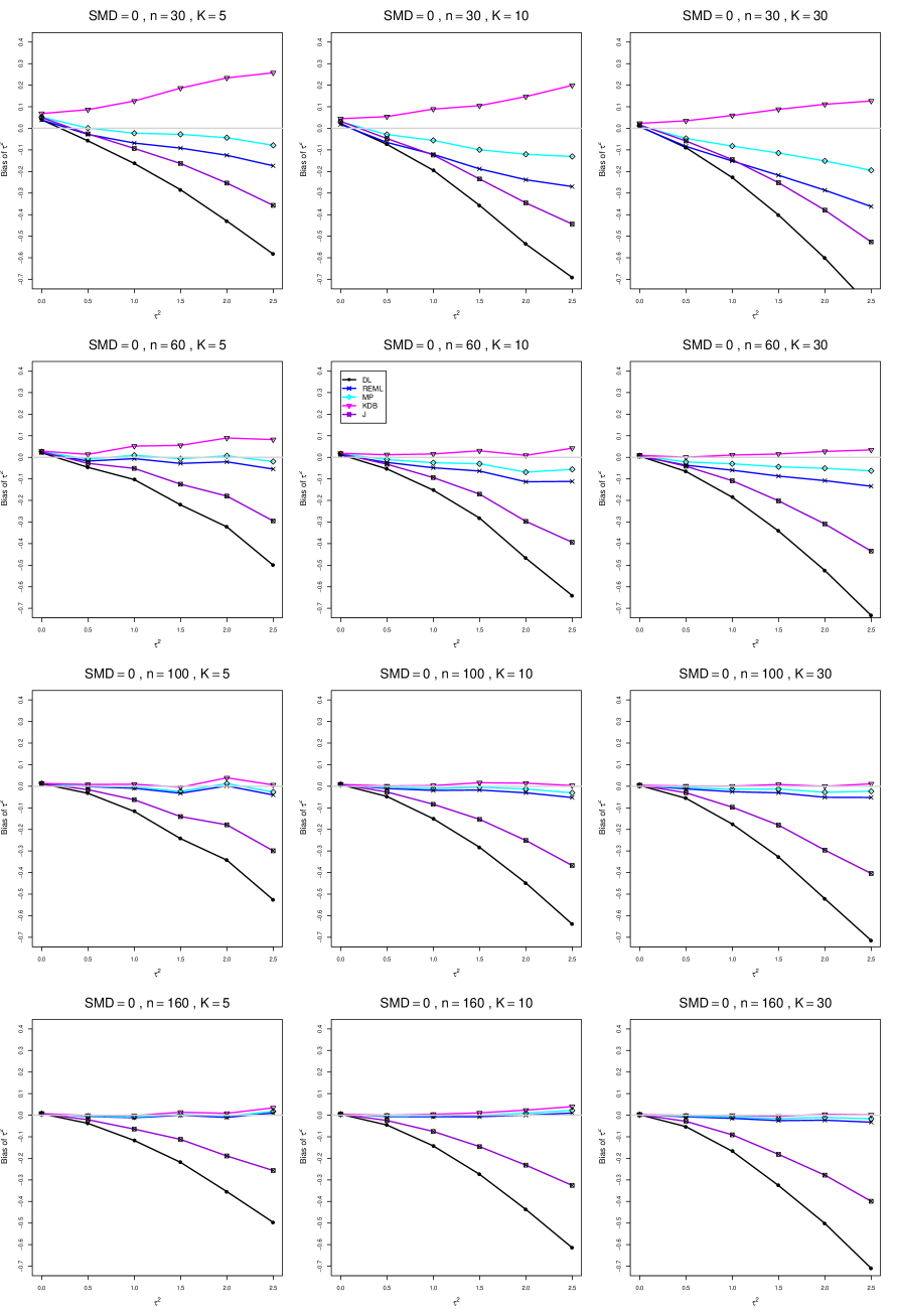
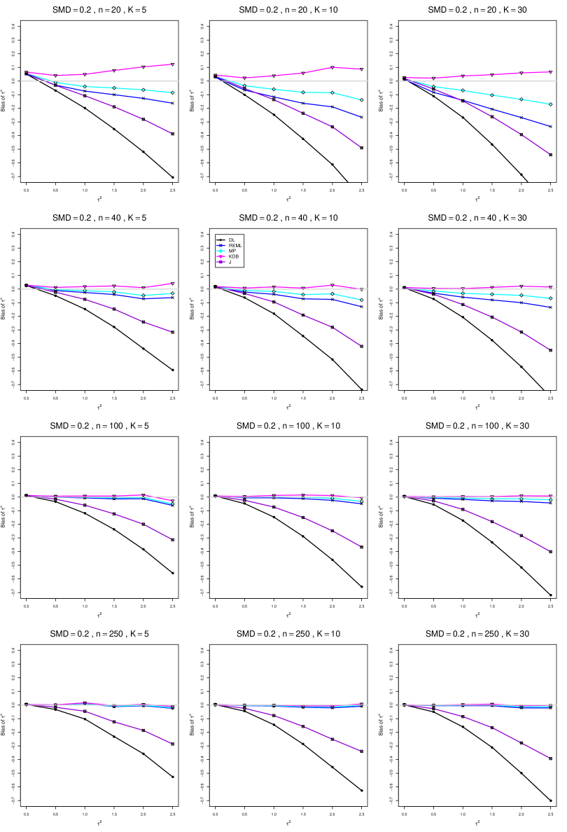
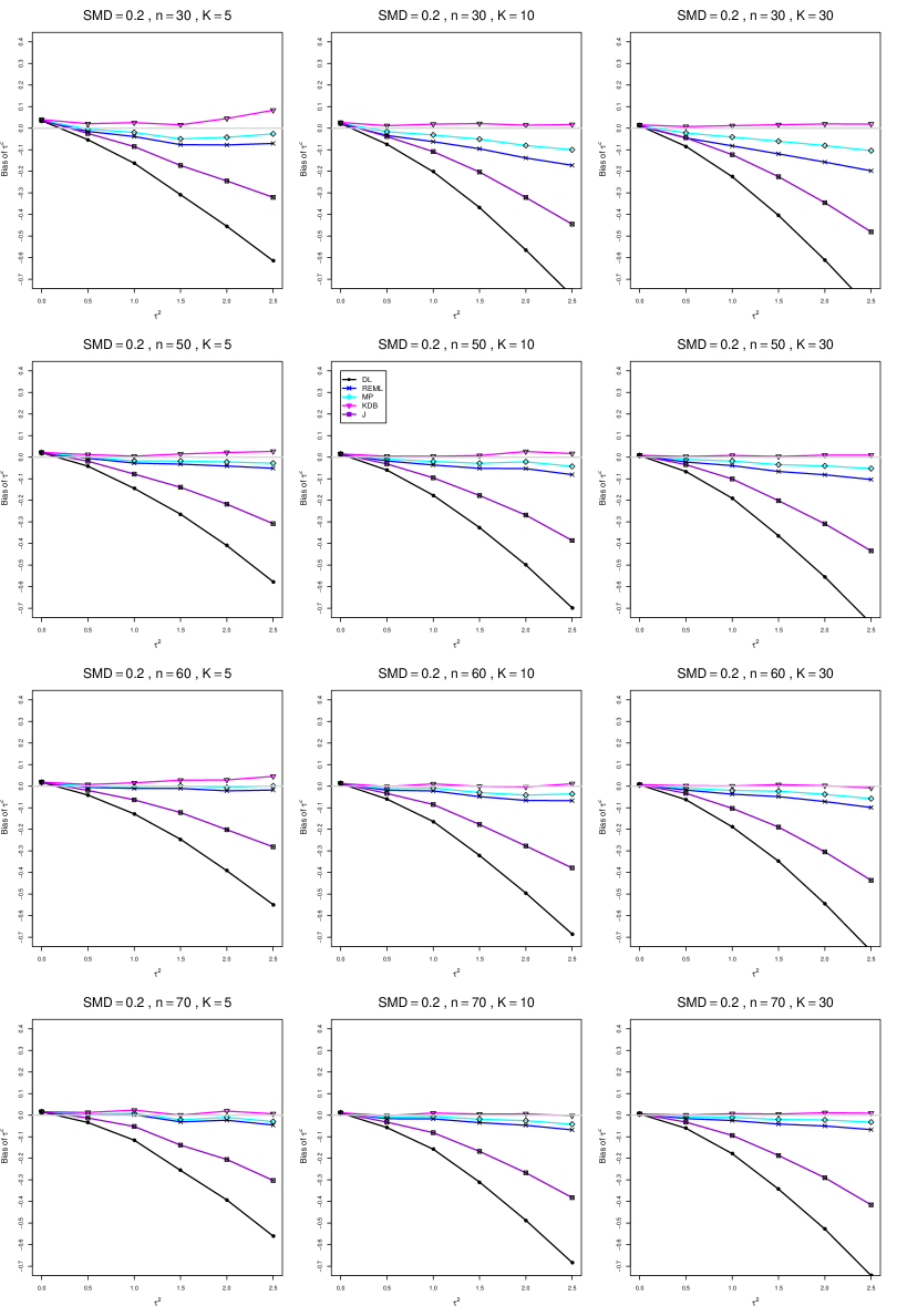
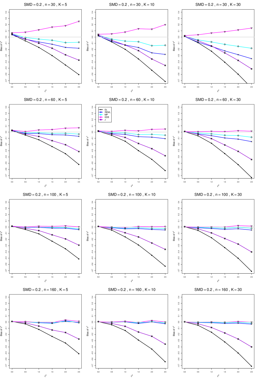
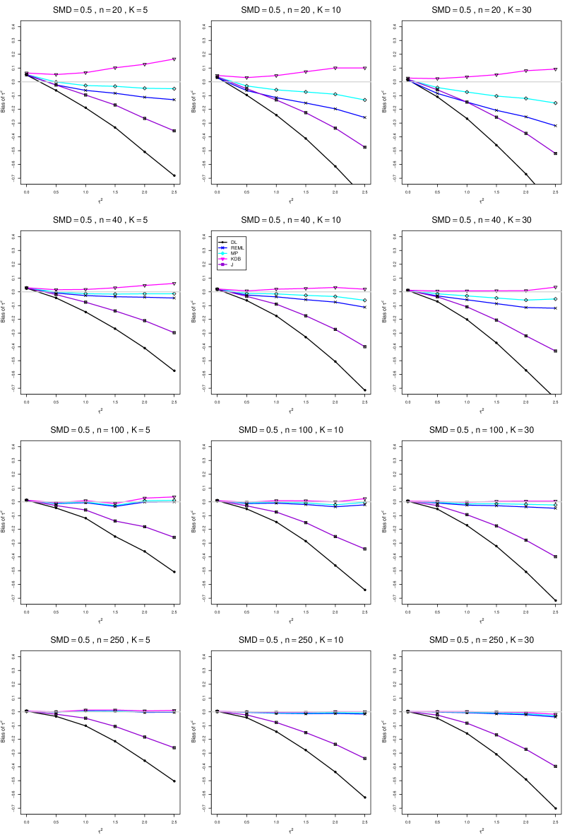
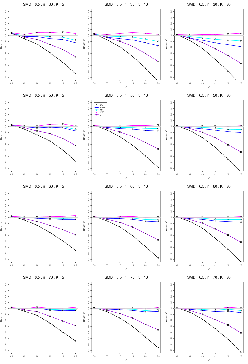
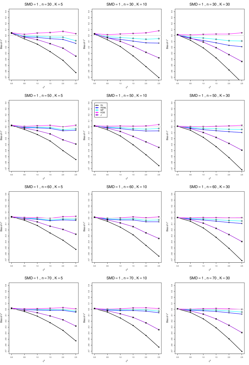
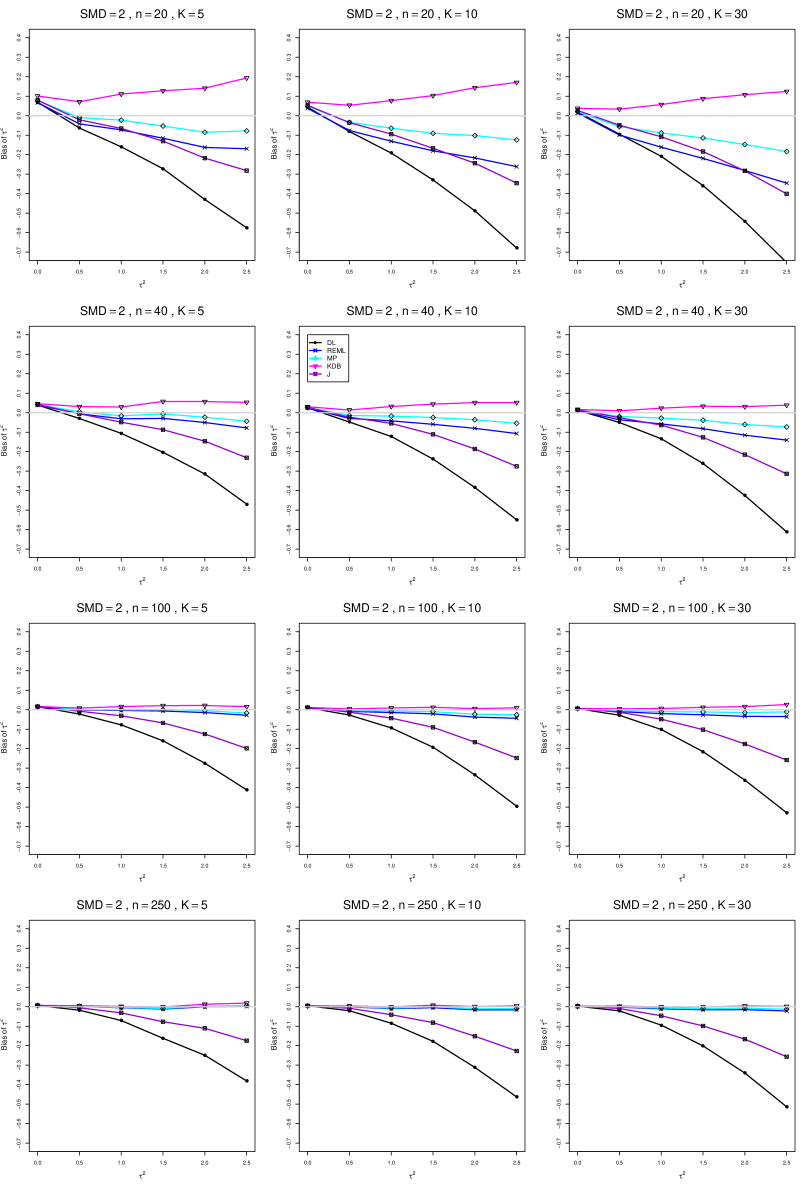
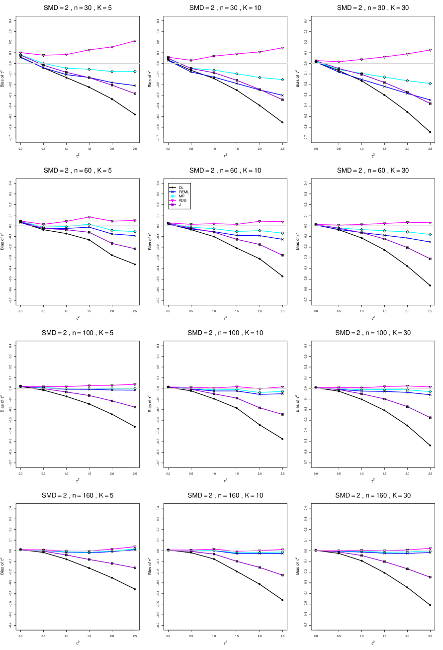
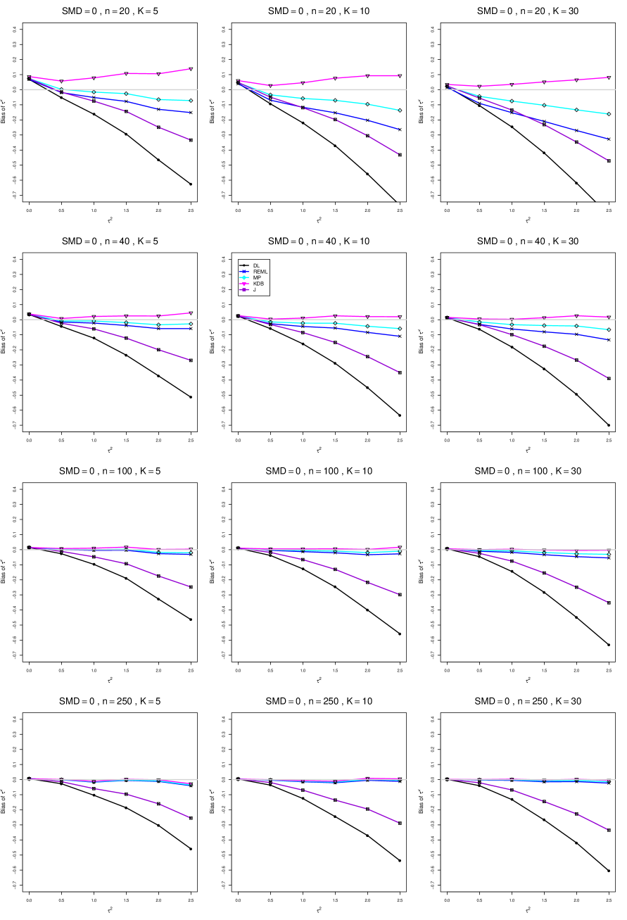
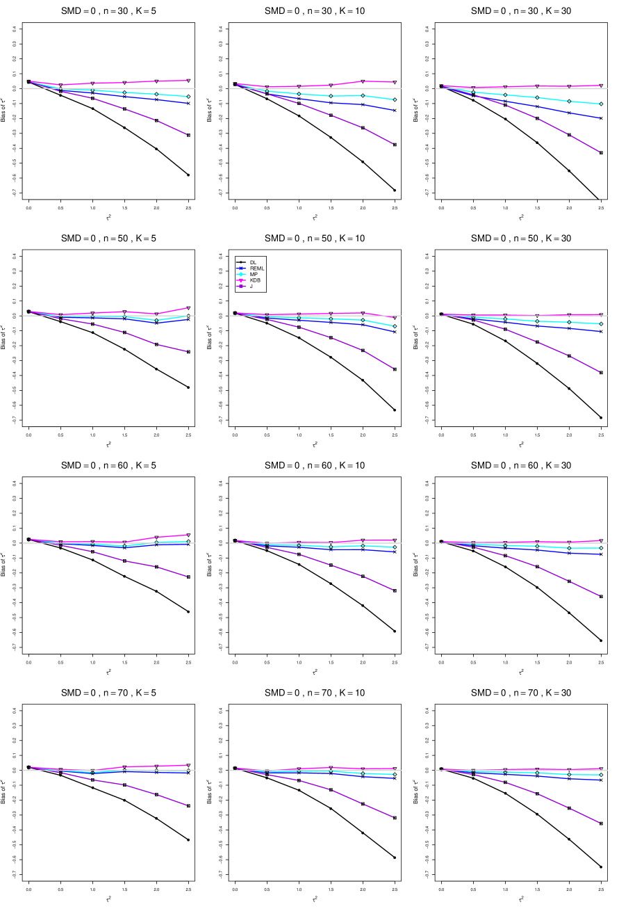
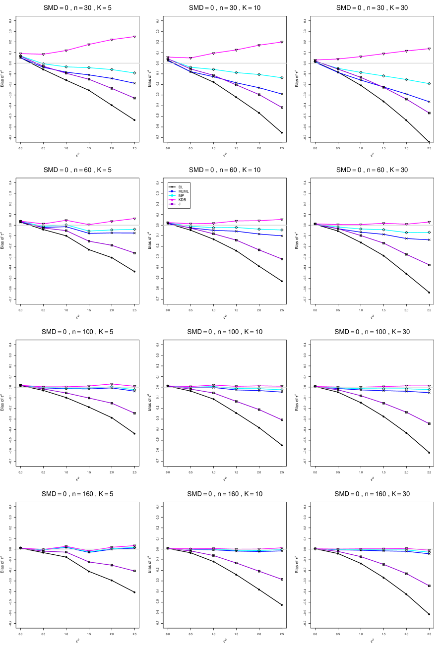
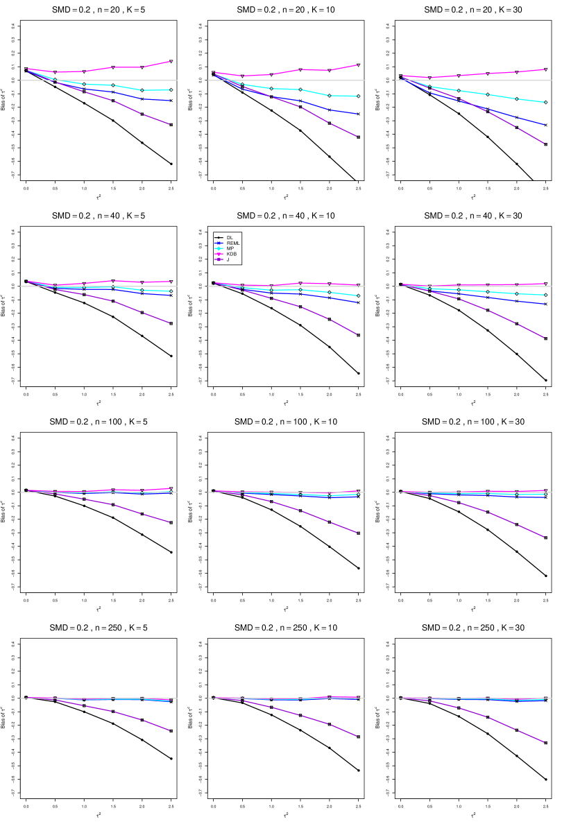
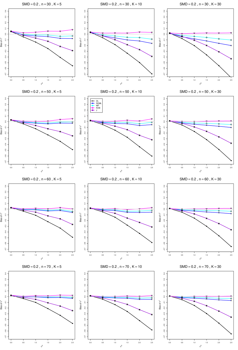
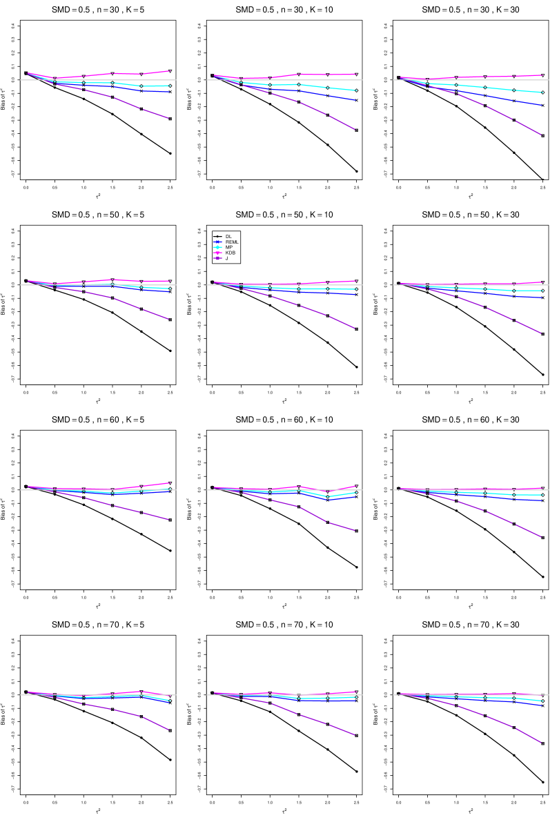
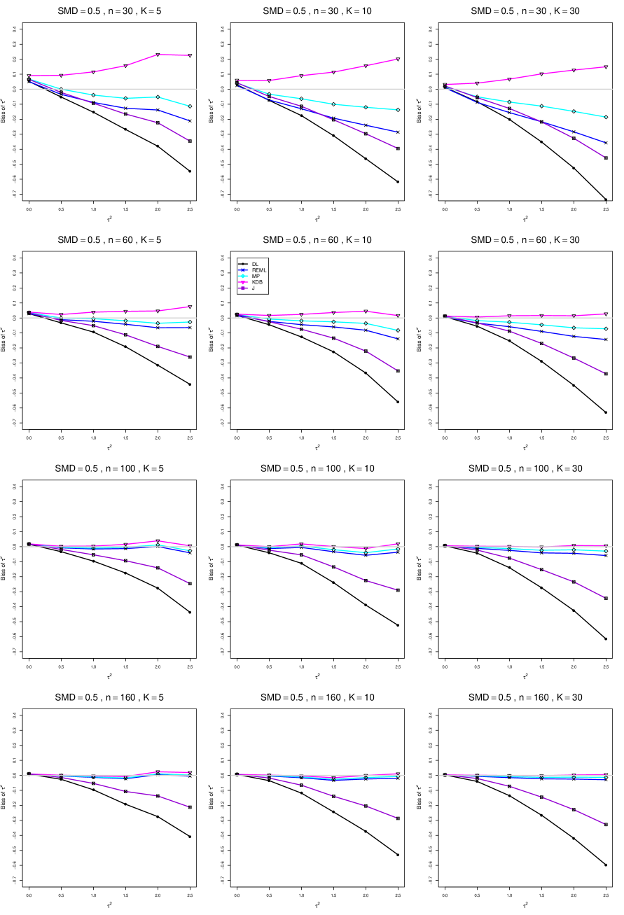
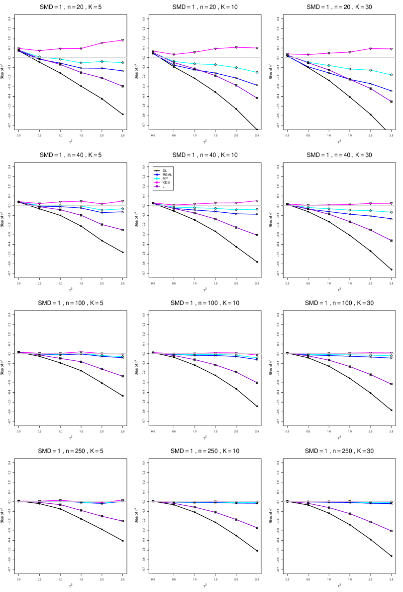
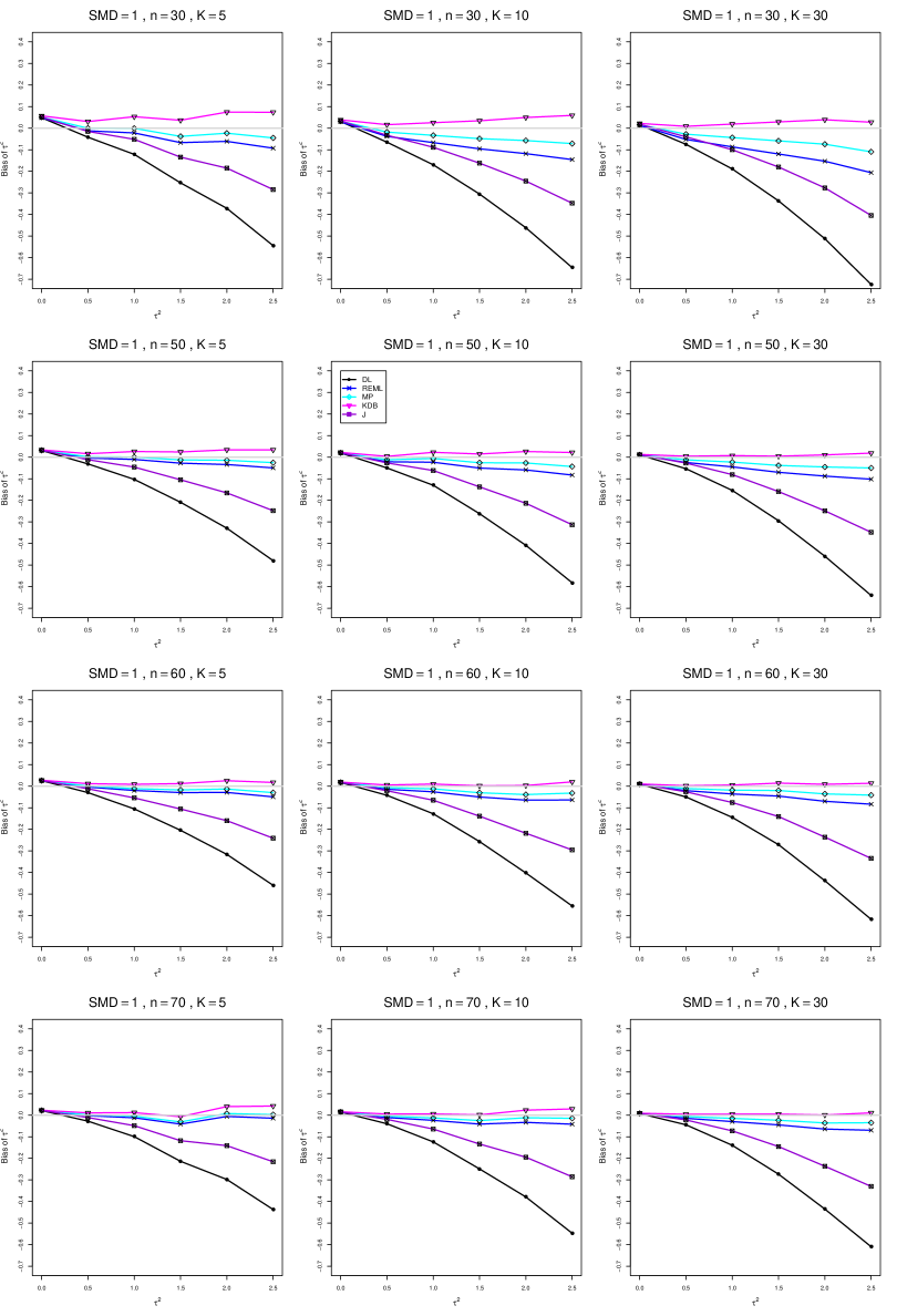
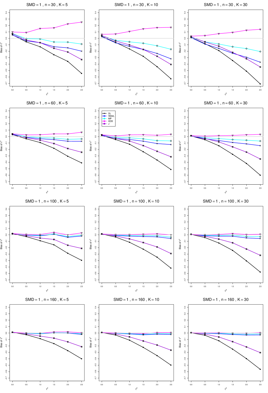
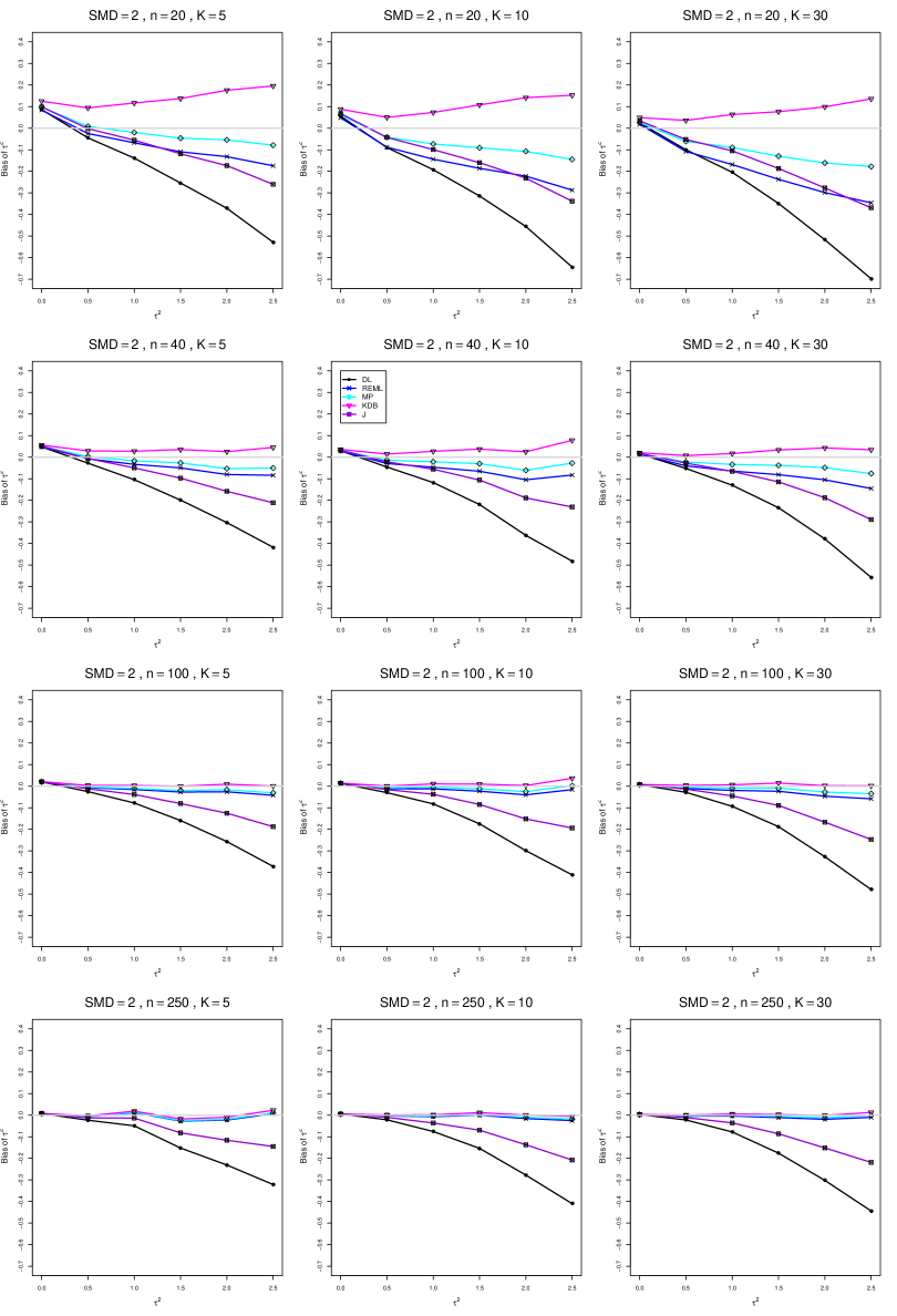
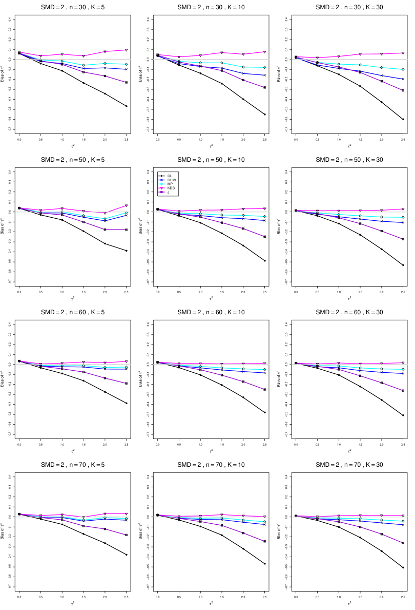
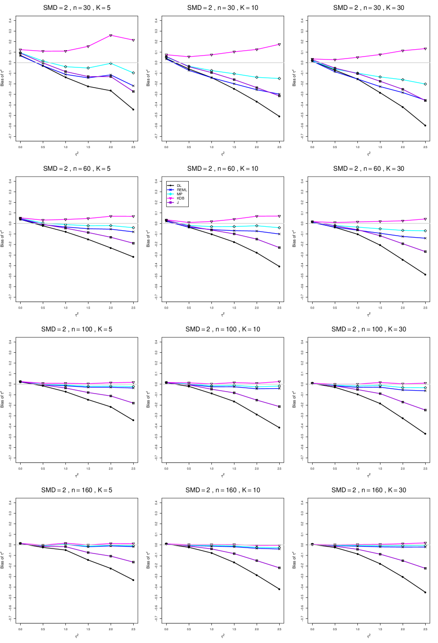
8.1 Bias in estimation of (Appendix A1)
The five estimators (DL, REML, J, MP, and KDB) have biases whose traces fan out from the same small positive bias at . As increases, KDB remains positive and increases slowly; MP stays close to 0 (and slightly below); REML stays negative, with a negative slope; J stays negative, with a more-negative slope; and DL becomes increasingly negative, showing noticeable curvature. The value of has little effect on this pattern (except that the bias of DL and J has smaller magnitude when ).
As or increases, the traces for KDB, MP, and REML flatten, and their bias is essentially 0 when or . The traces for J and DL become less steep, but substantial bias remains at (or ).
As increases, the trace for KDB flattens somewhat, but the traces for the other estimators become steeper.
The traces for J and DL are slightly less steep when than when .
In summary, the patterns of bias indicate a choice among the five estimators of (DL, REML, J, MP, and KDB). When , MP is closer to unbiased than KDB when , the magnitudes of their biases are roughly equal when , and KDB is closer to unbiased when . When , MP, KDB, and REML are nearly unbiased. DL and J seriously underestimate . The average of MP and KDB should be close to unbiased.
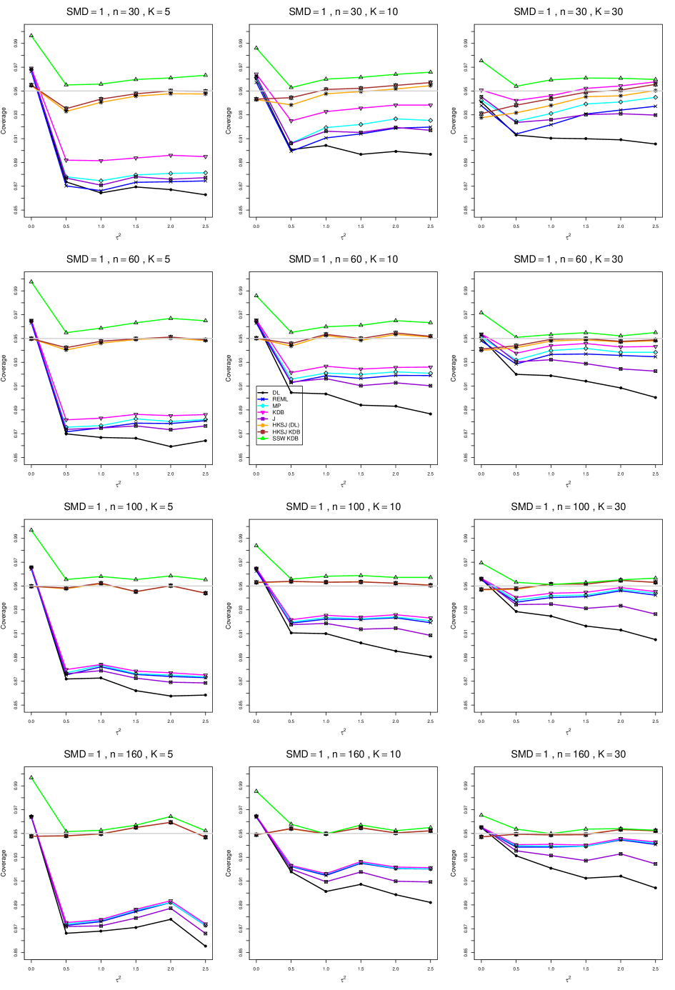
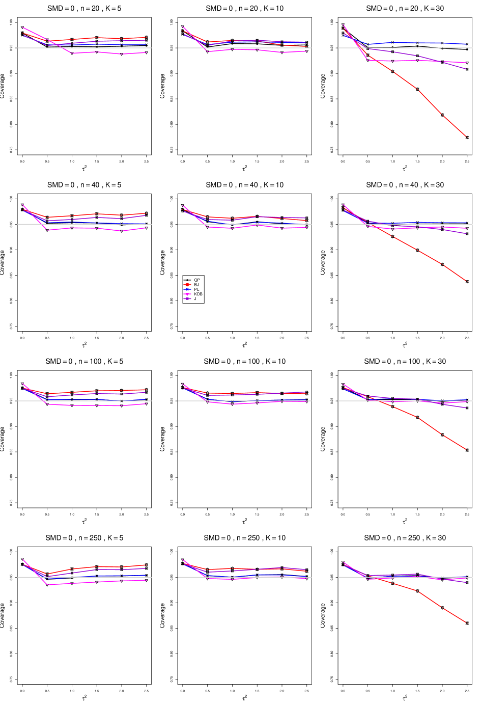
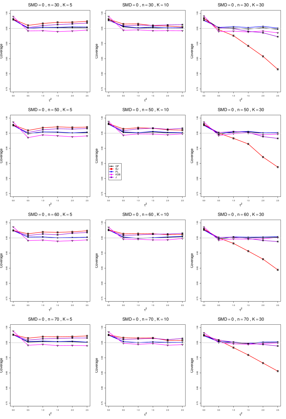
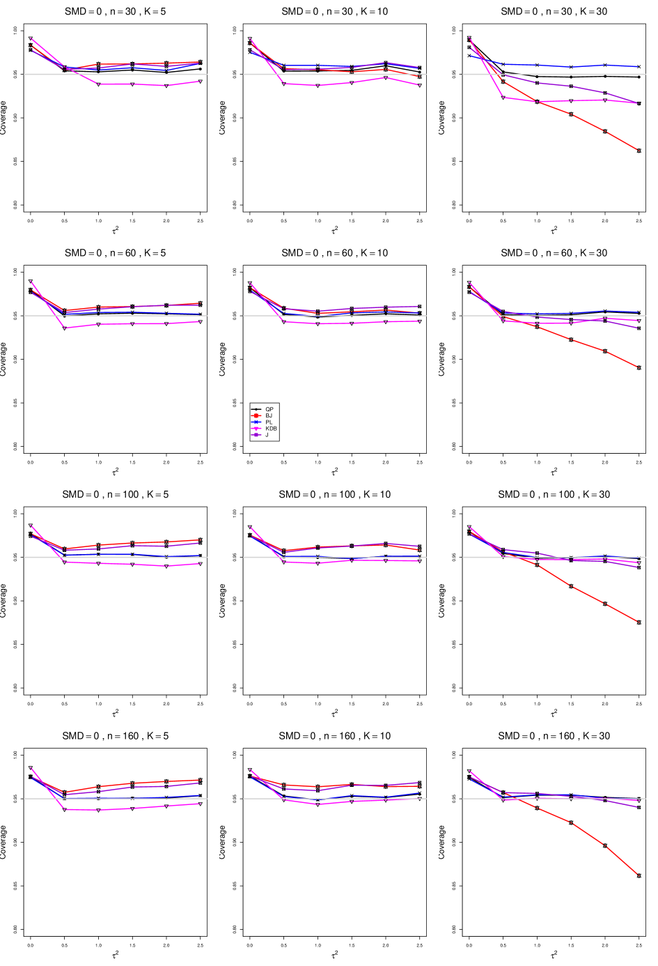
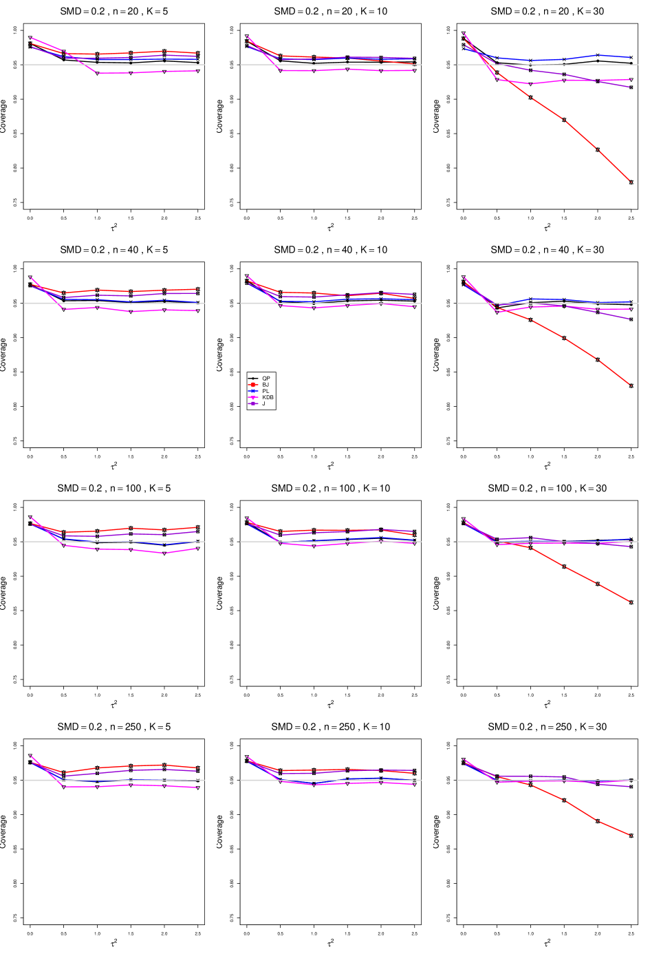
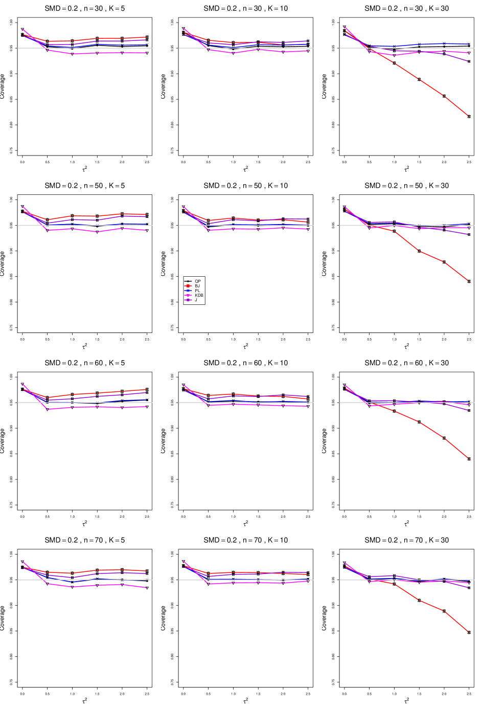
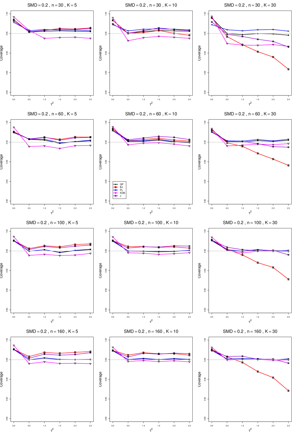
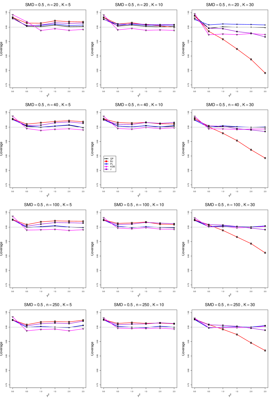
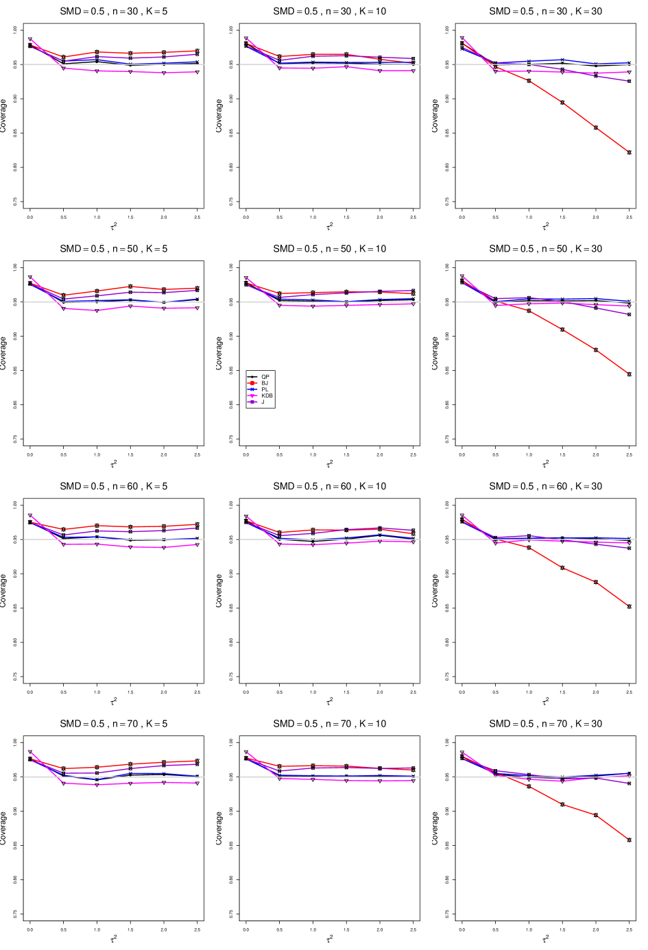
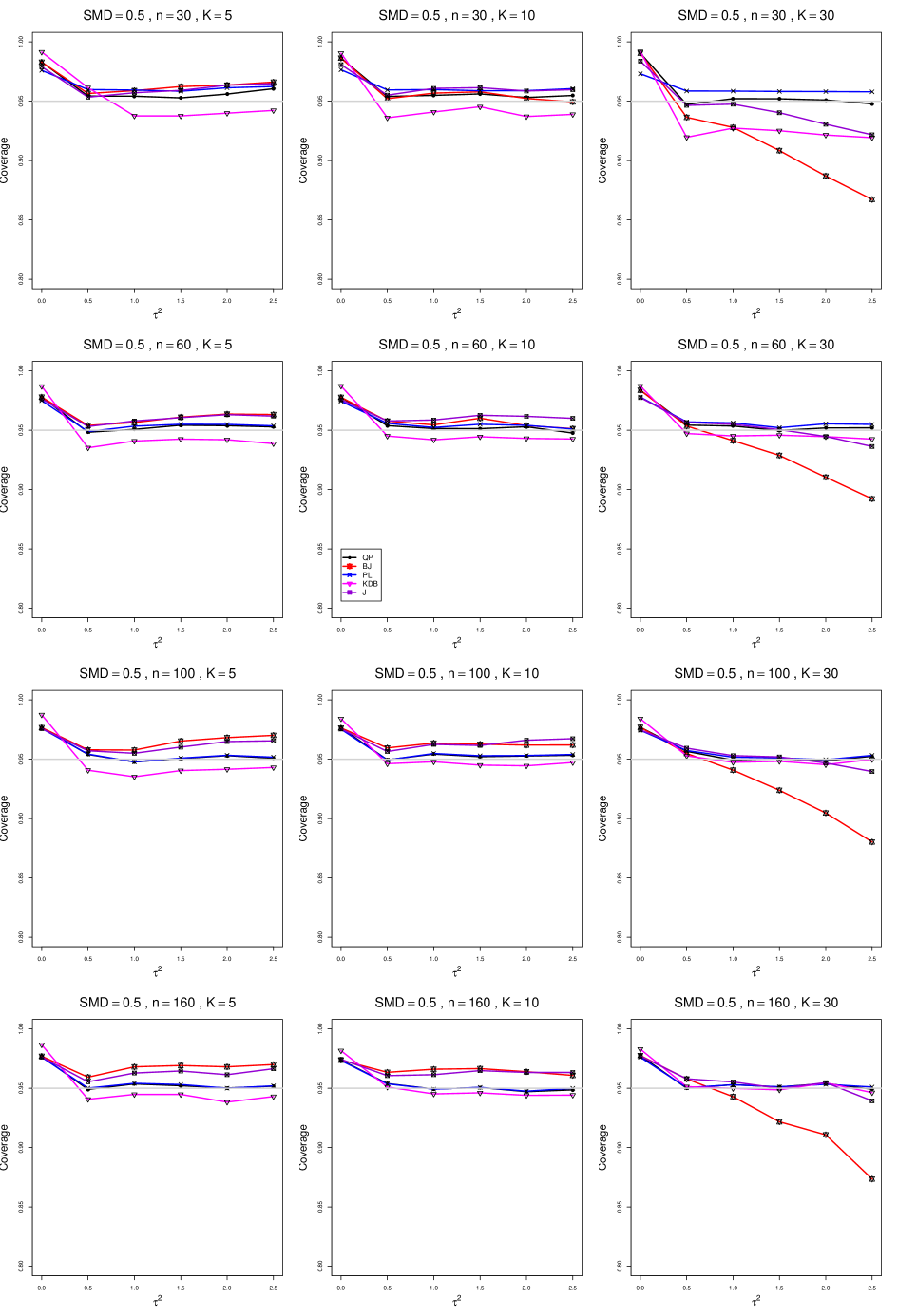
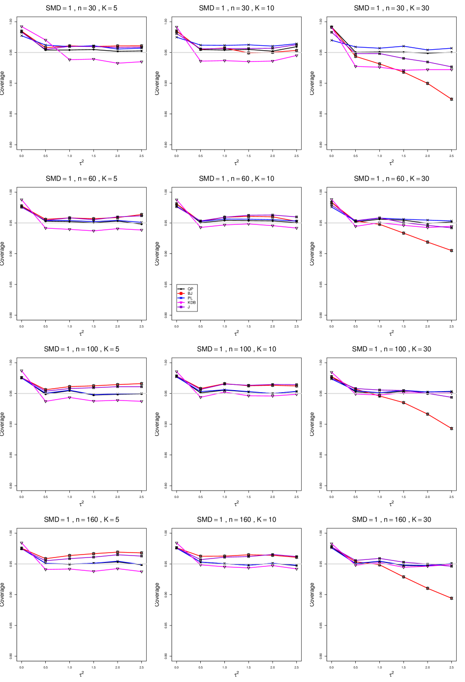
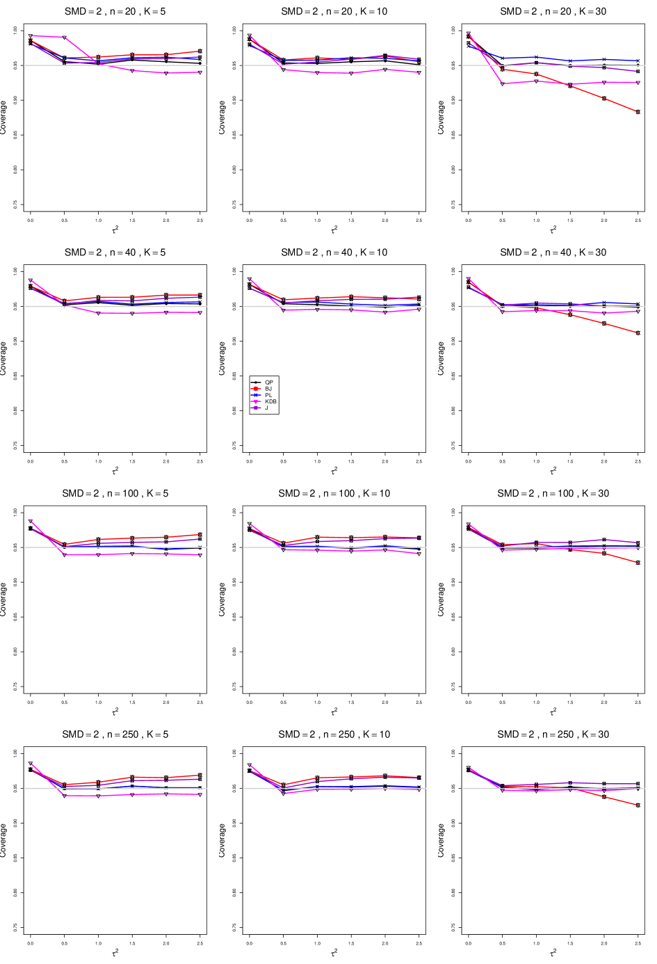
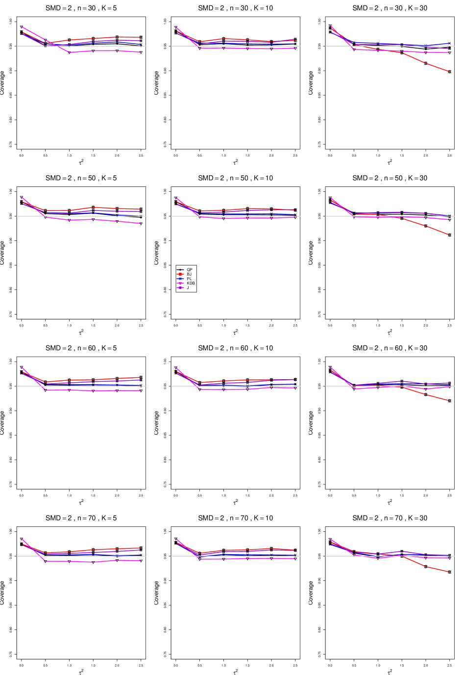
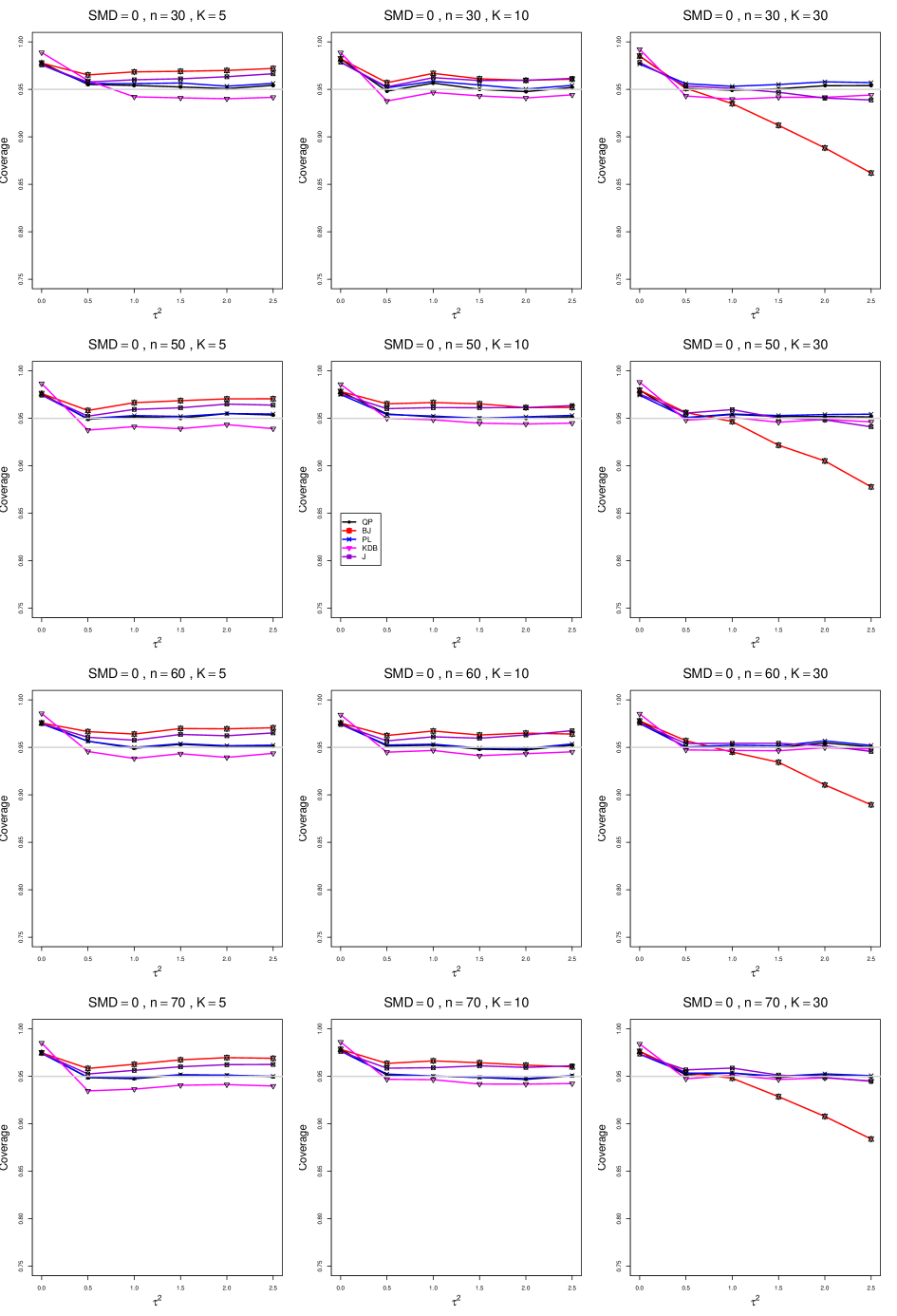
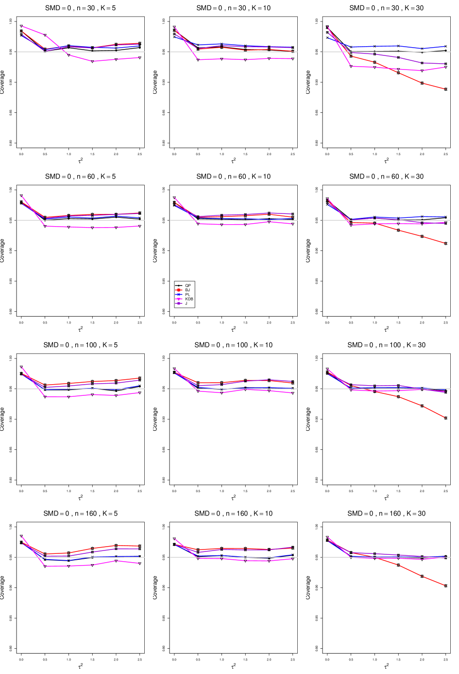
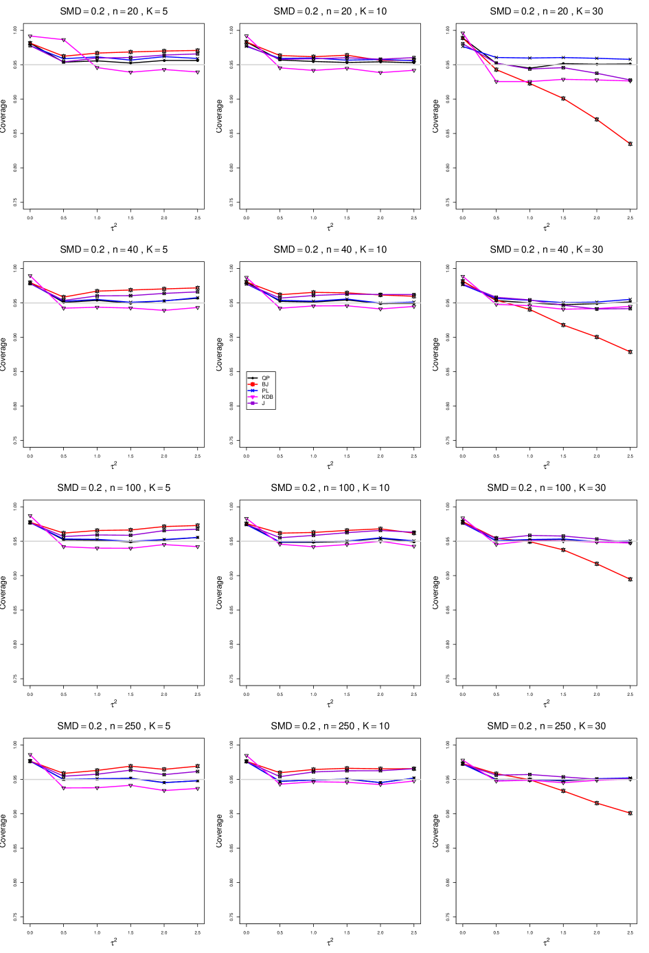
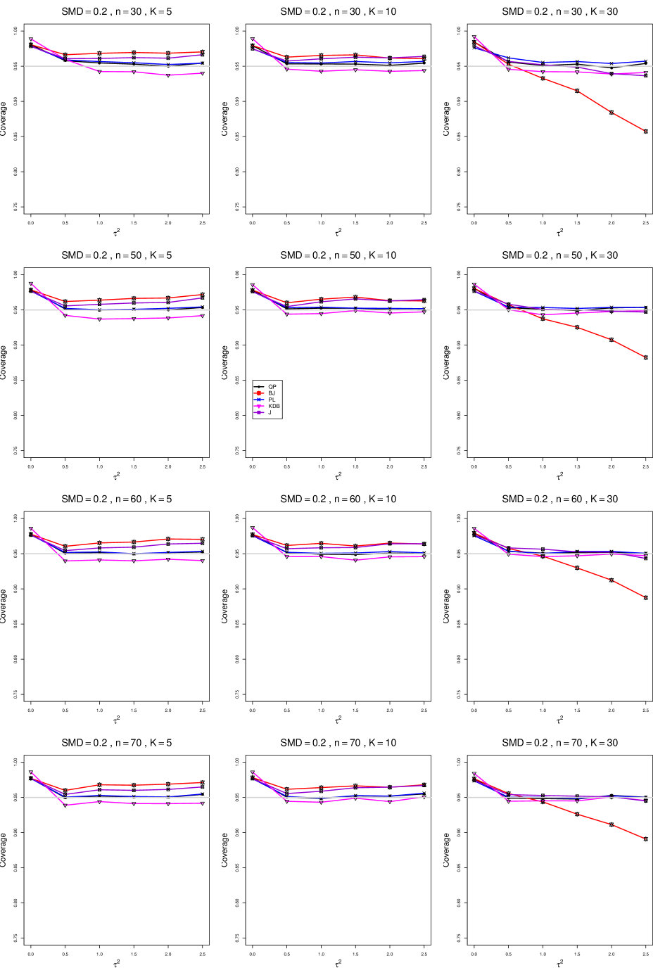
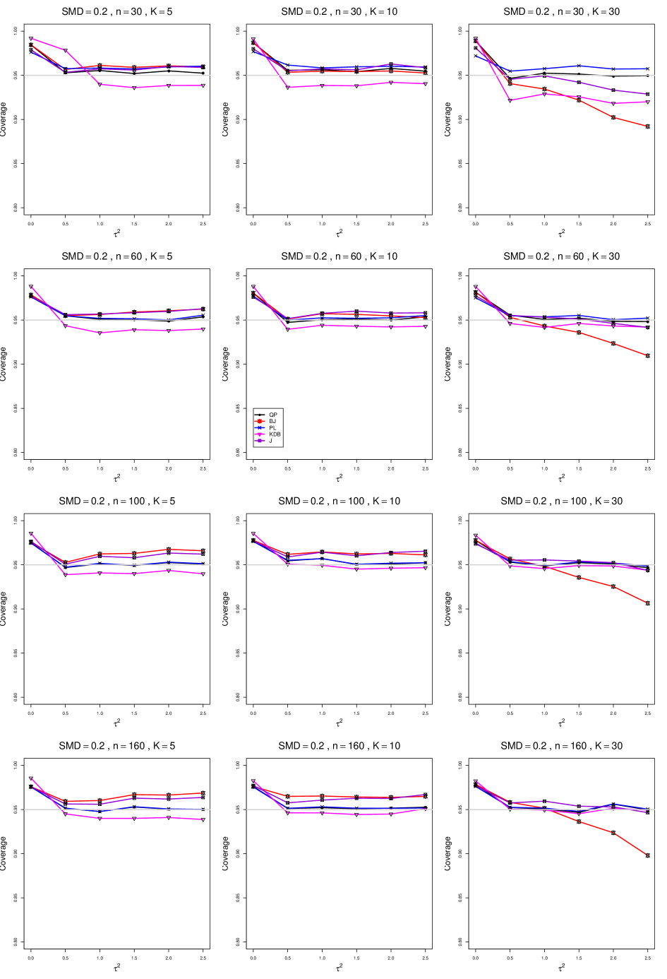
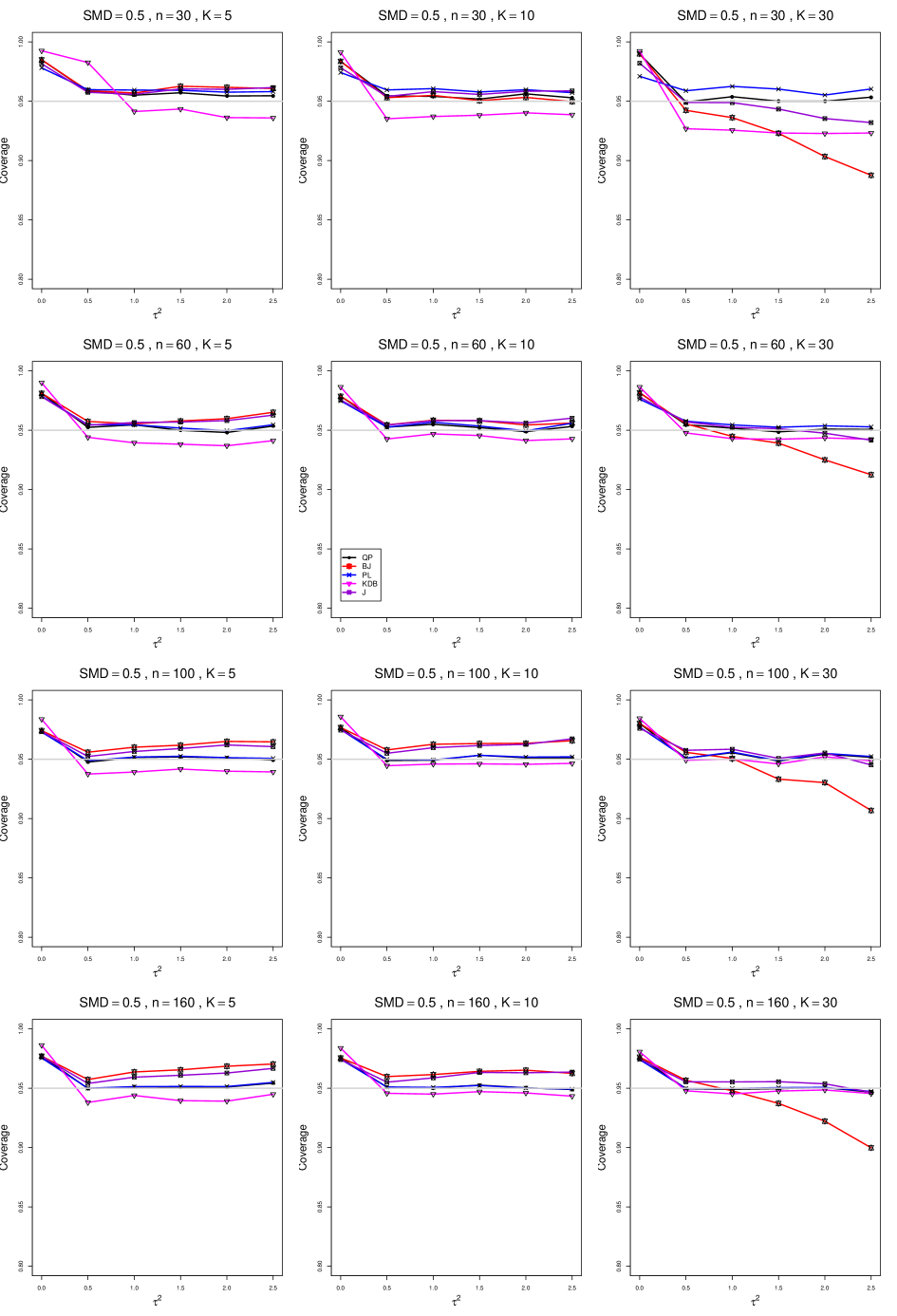
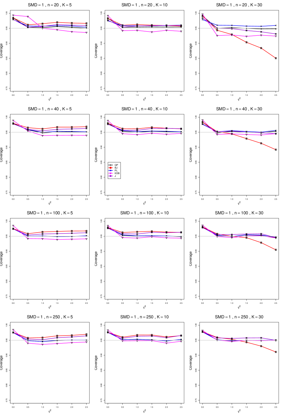
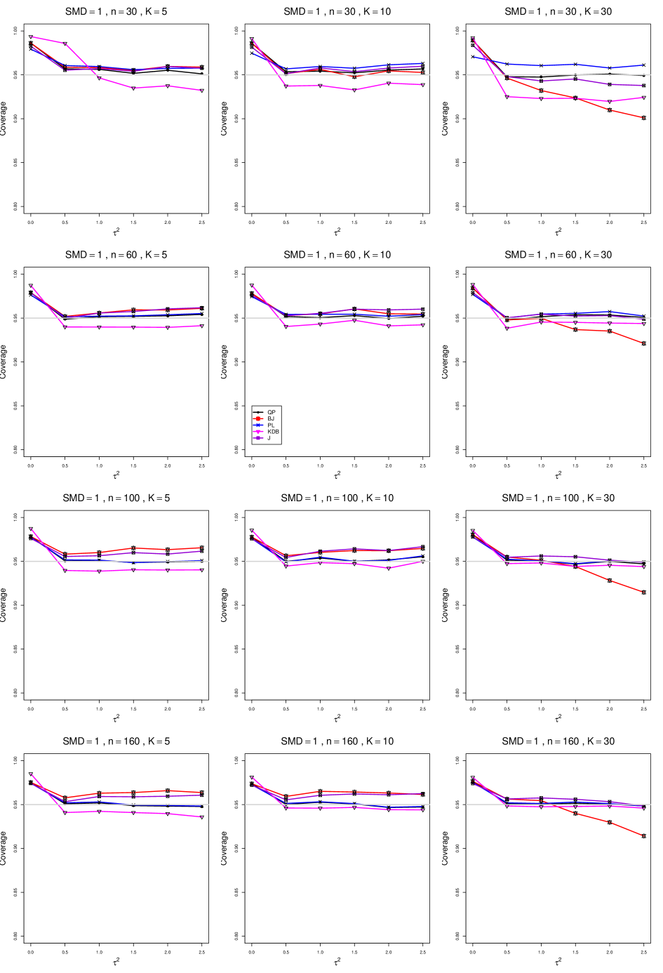
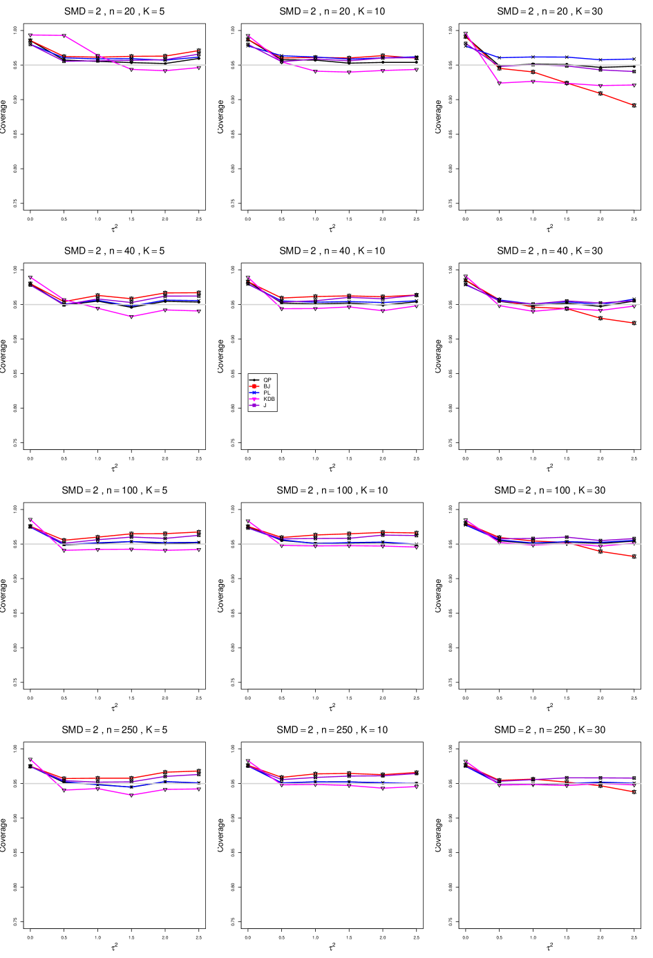
8.2 Coverage in estimation of (Appendix A2)
The five estimators (PL, QP, BJ, J, and KDB) share the feature that their coverage decreases as increases from 0 to 0.5. At all five have coverage . KDB is highest (e.g., .99 when and ), but it drops below .95 at or and remains slightly below .95. BJ is next highest (e.g., .98 when and ), and it remains above .95 (say, .96 to .97) when and . QP is close to .95 for . PL is between BJ and QP, and it remains above QP when . The trace for BJ behaves quite differently when than when , decreasing steeply and linearly to around .77 at (when and ). When , J is between BJ and QP; and when , it also decreases linearly, but less steeply (e.g., to around .92 at when and ).
Coverage does not change noticeably as or increases, when . When , the slopes of BJ and J become slightly less steep, and the traces of the other estimators move closer together and are closer to .95.
Setting aside the behavior of BJ and J when , and of the other estimators when and , the traces move closer together as increases.
The slopes of BJ and J when are less steep when than when .
As increases, the coverage of QP at increases slightly; it is substantially closer to .95 when .
In summary, all five interval estimators of have coverage substantially above .95 when . When , QP is generally closest to .95. The unusual behavior of BJ (and, to a lesser extent, J) when adds to the evidence against it.
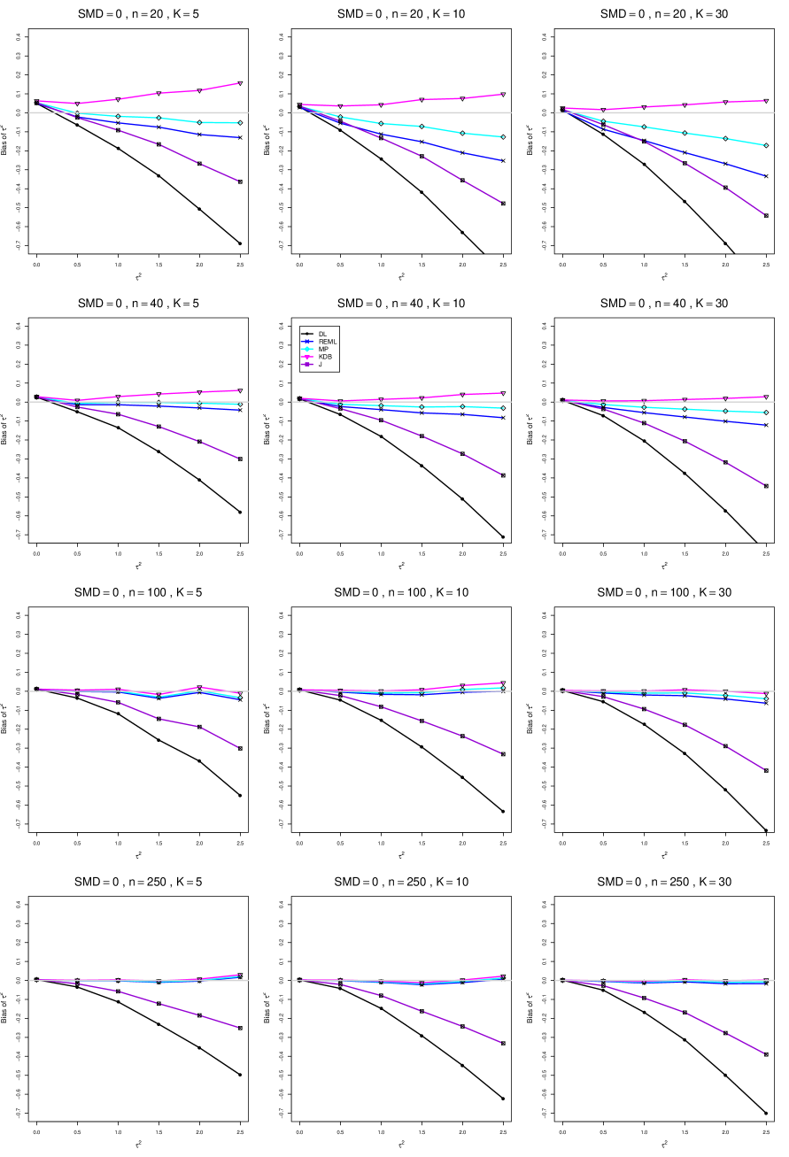
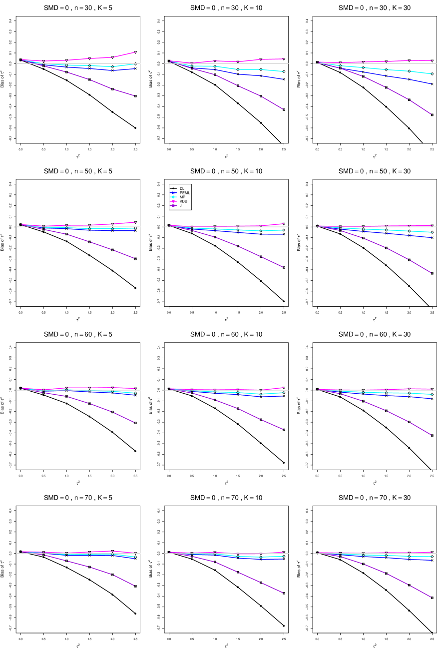
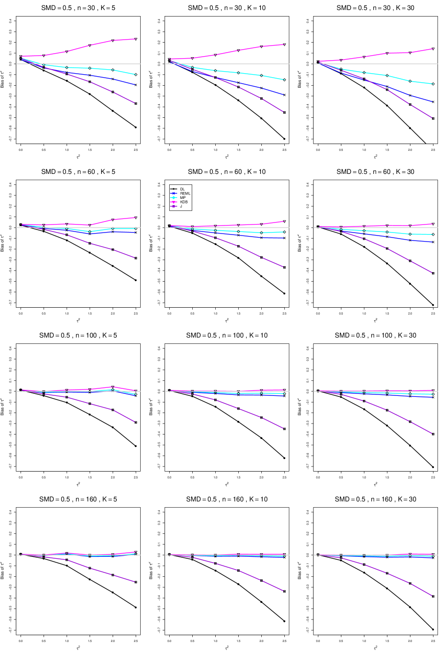
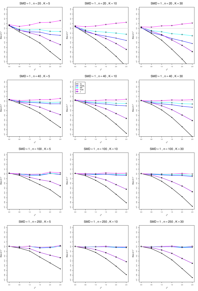
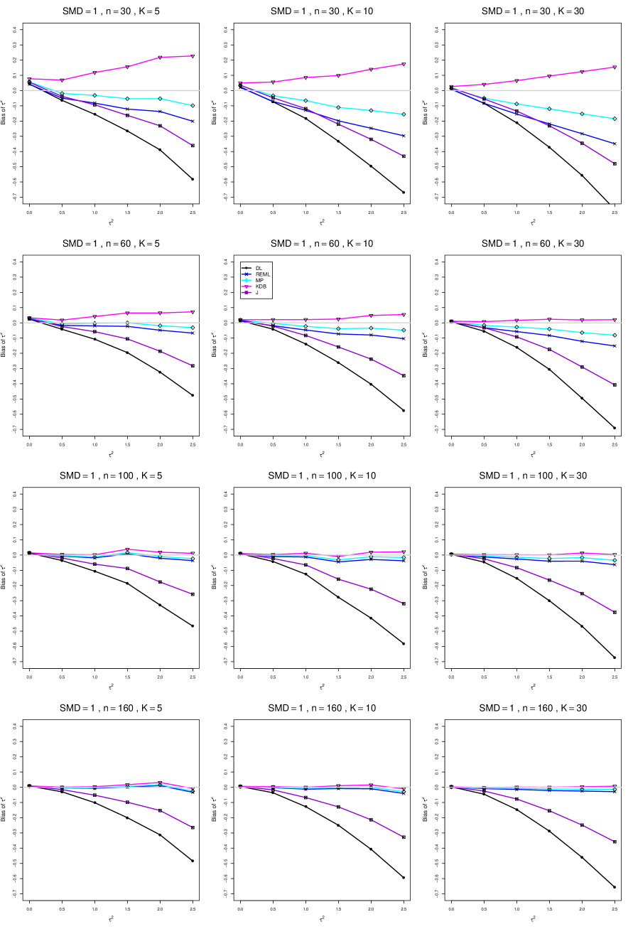
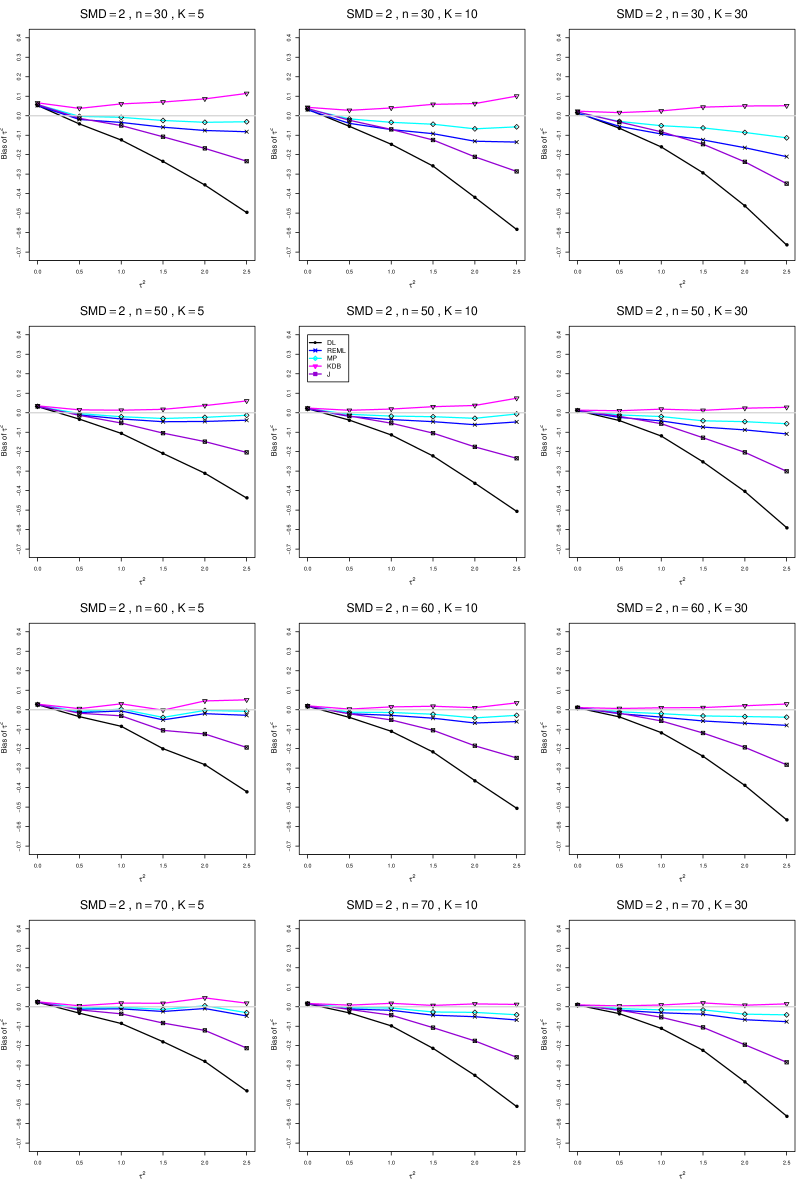
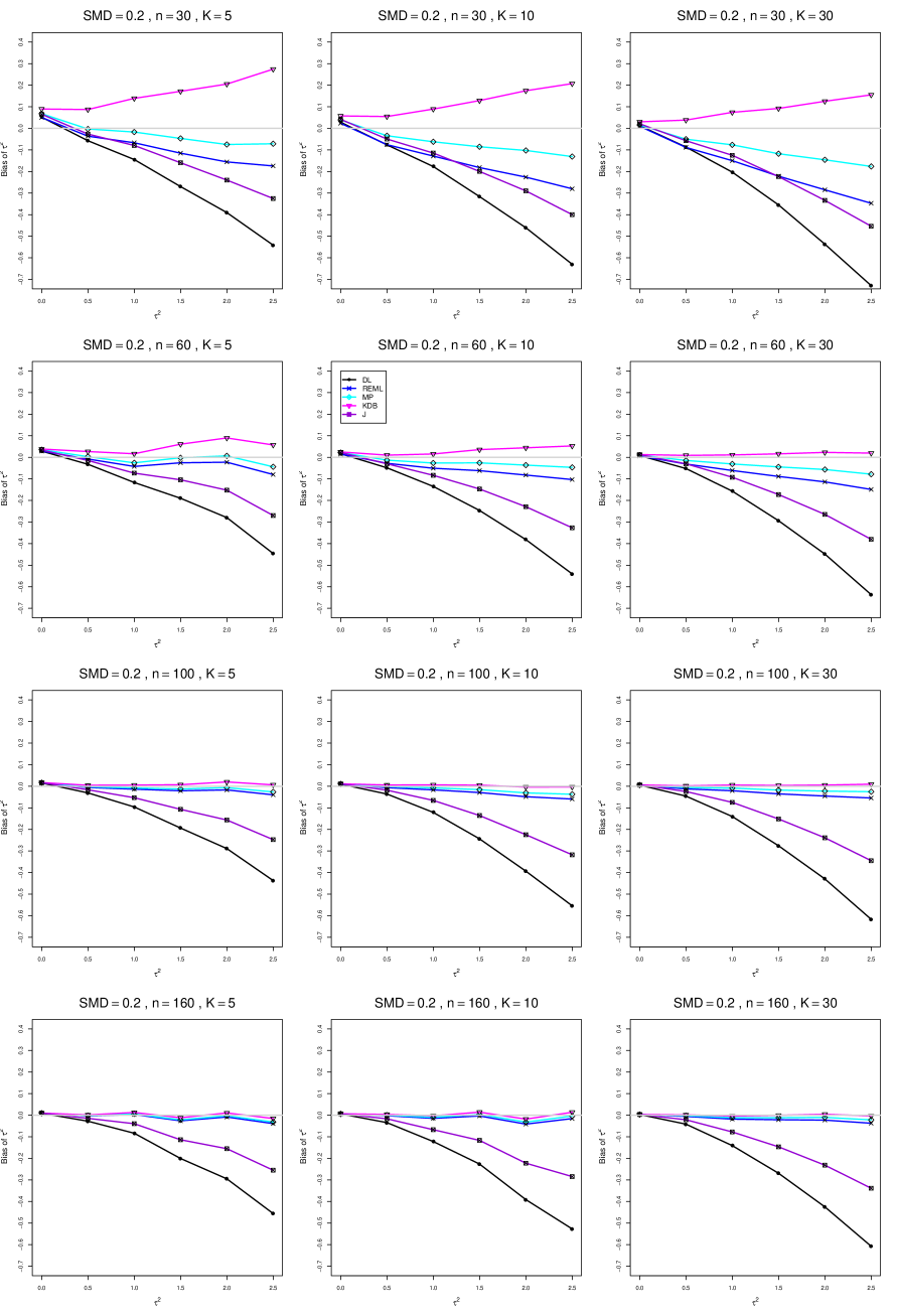
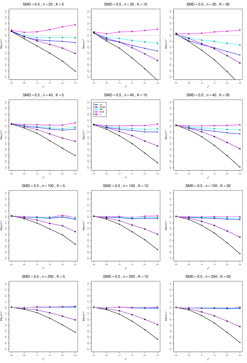
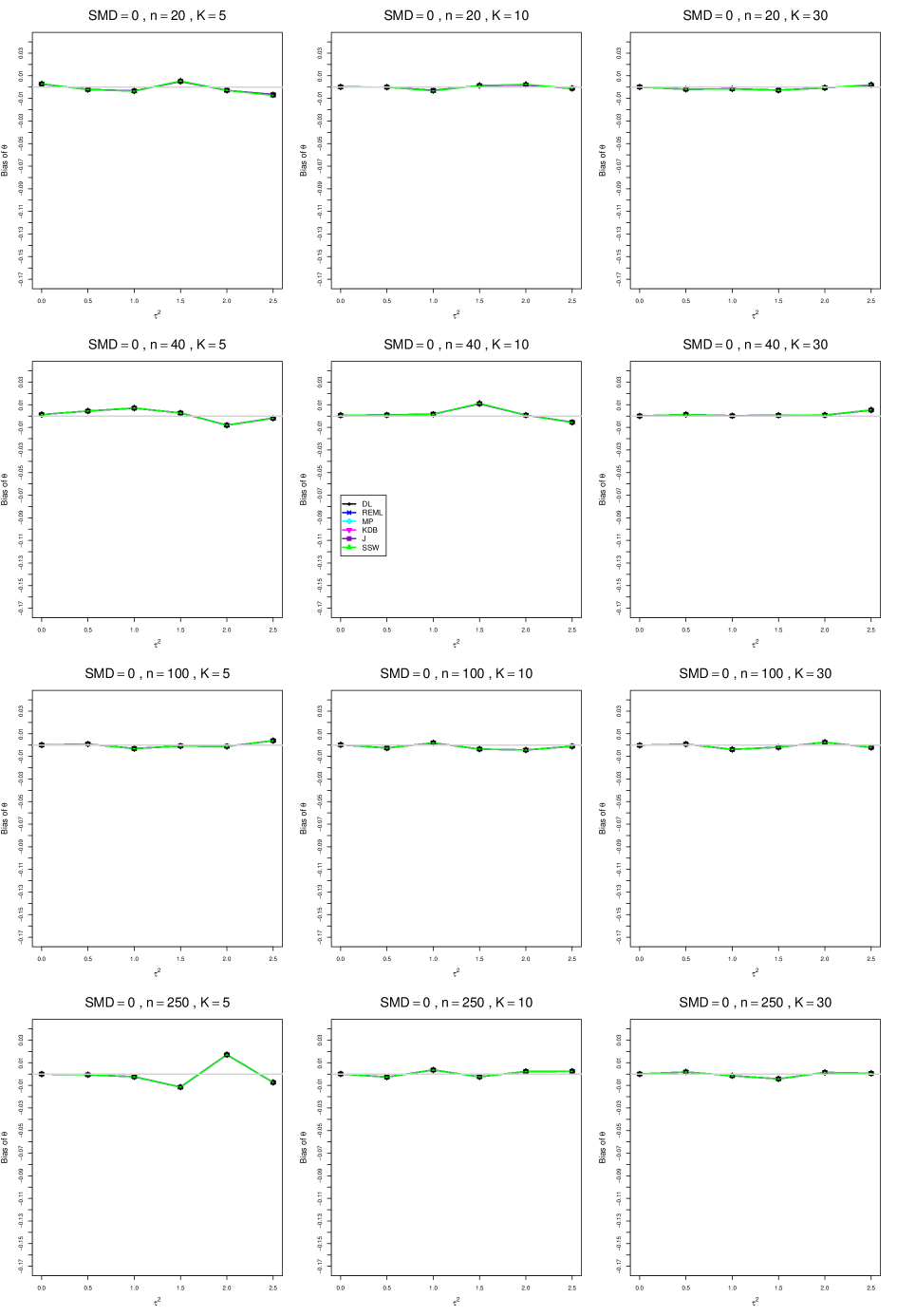
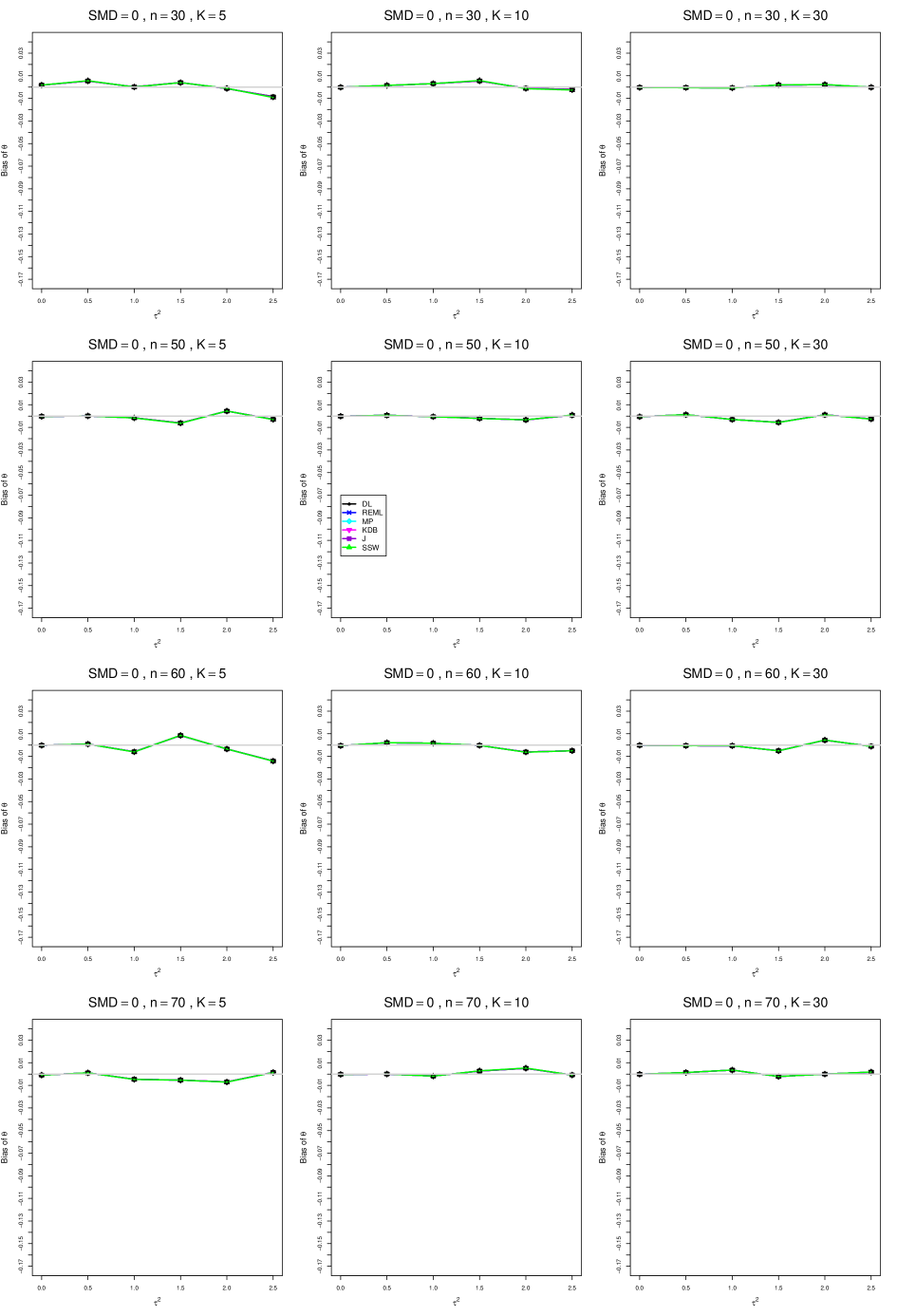
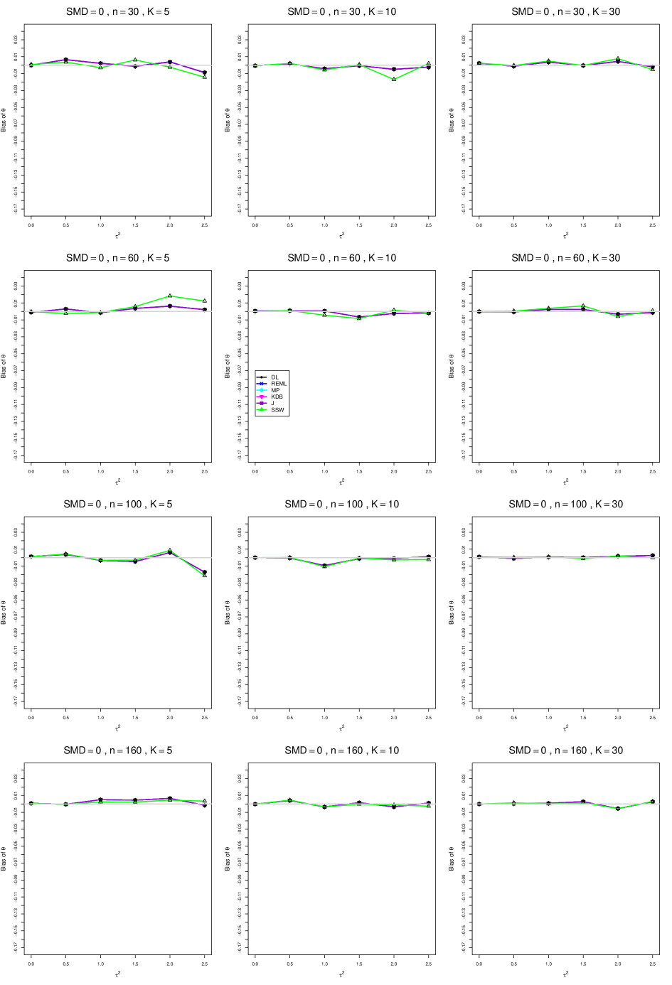
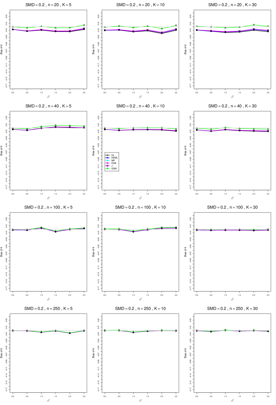
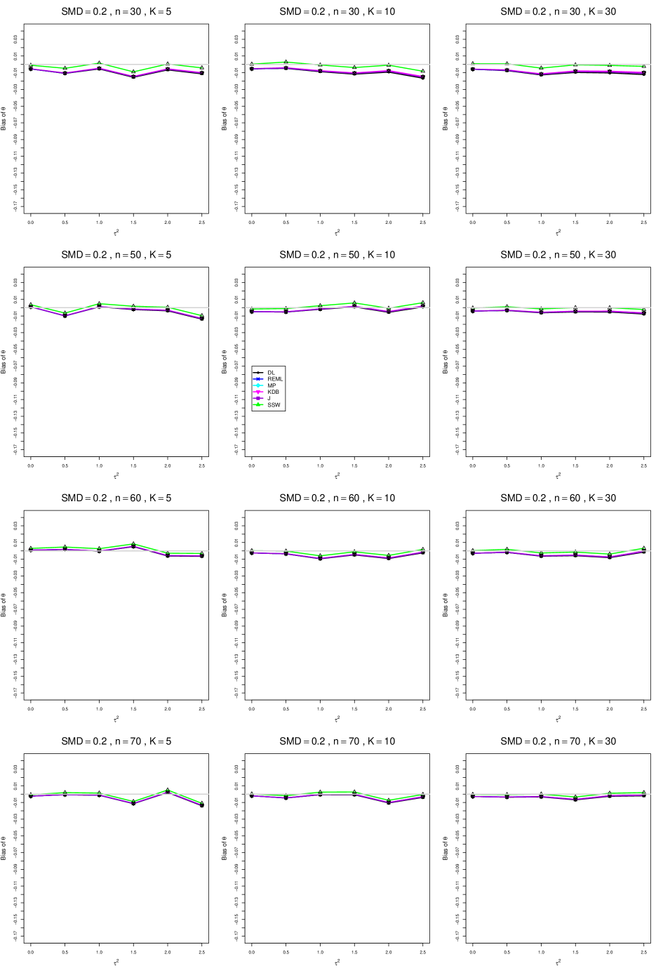
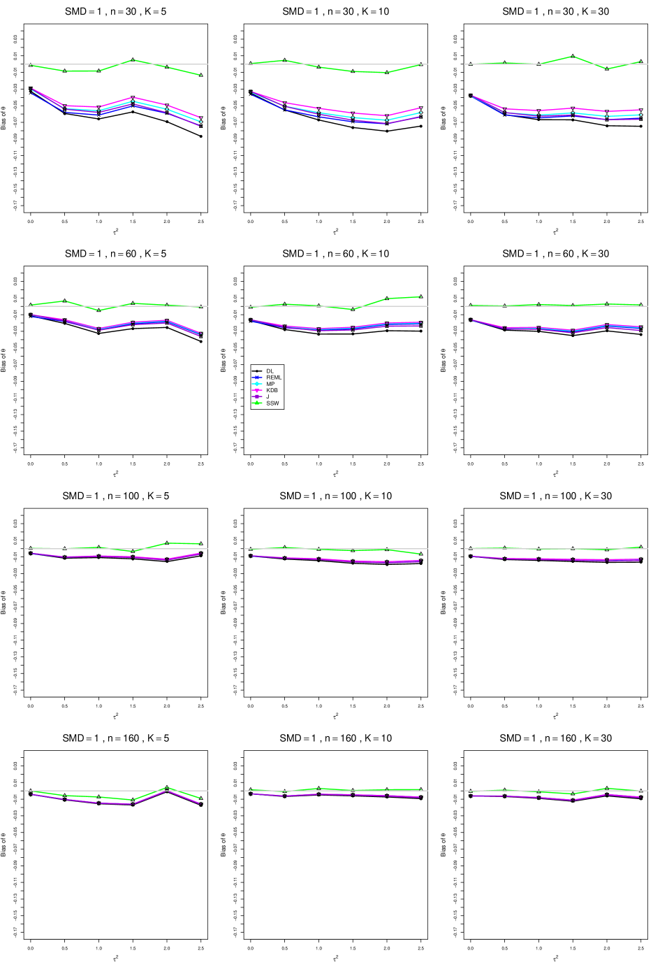
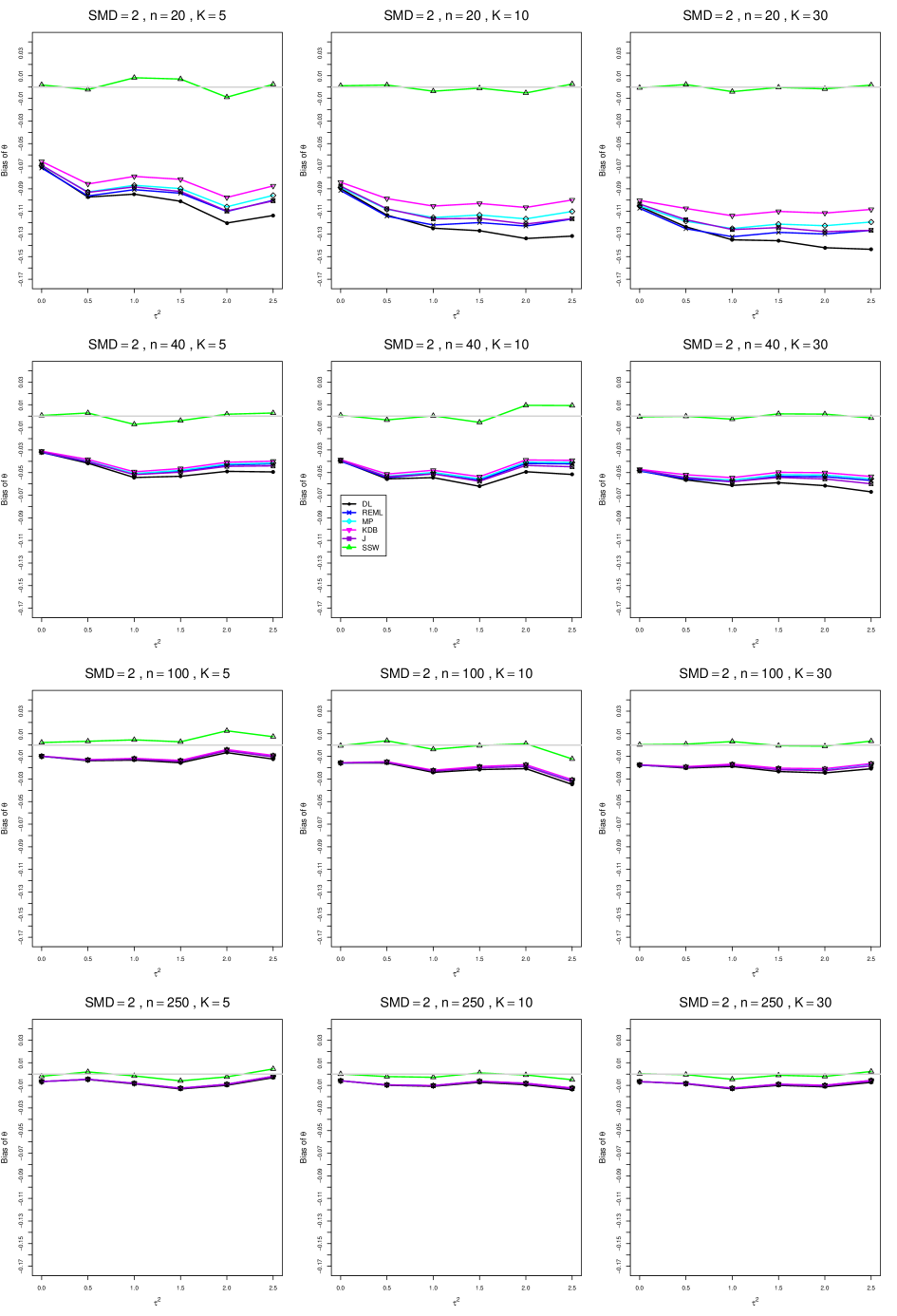
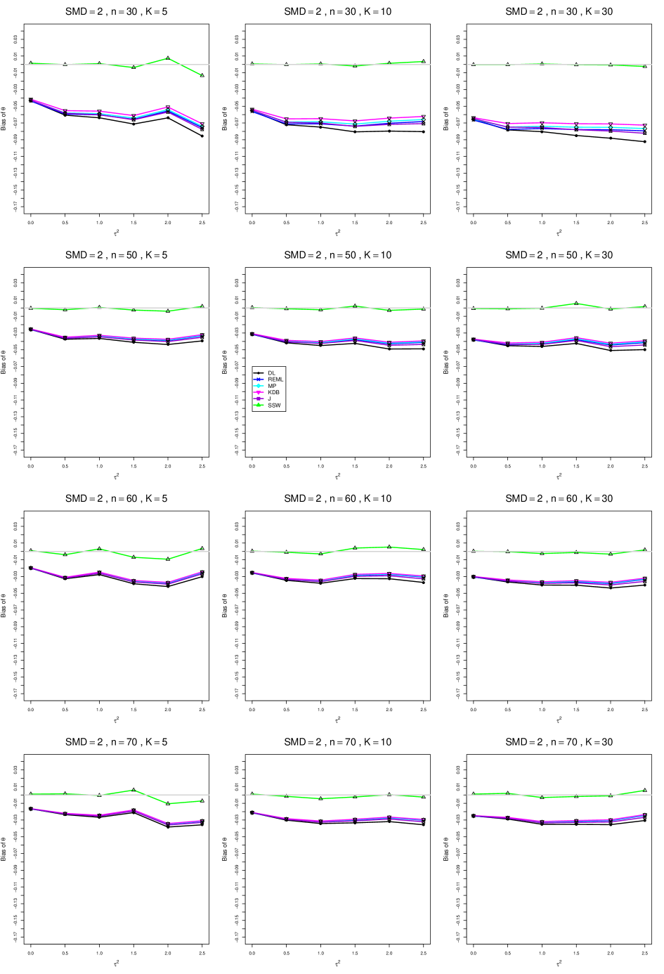
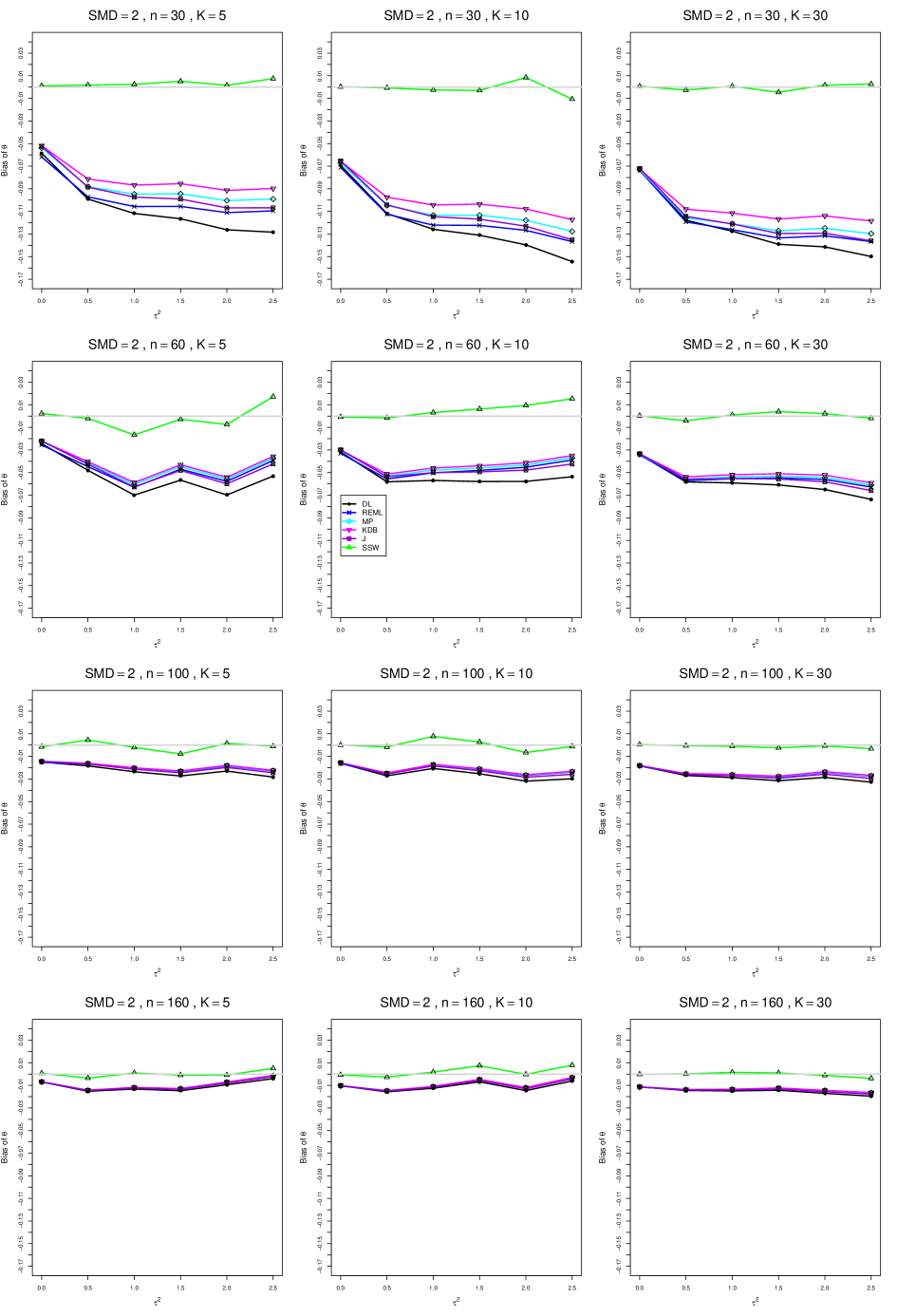
8.3 Bias and mean squared error in estimation of (Appendix B1)
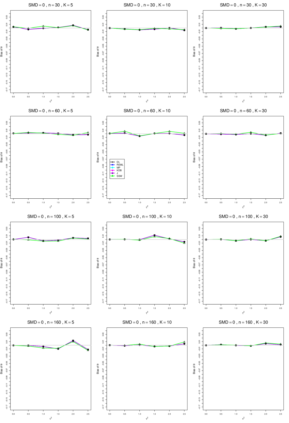
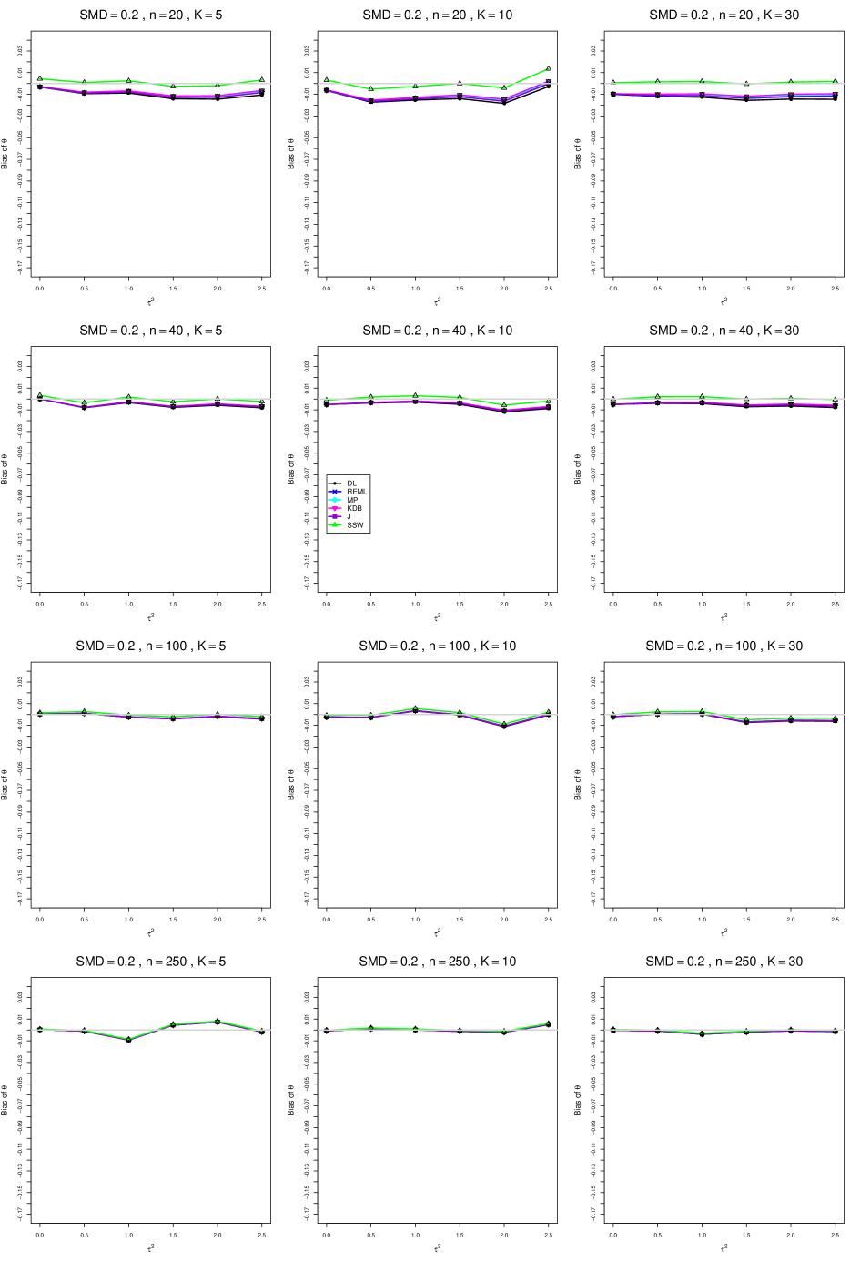
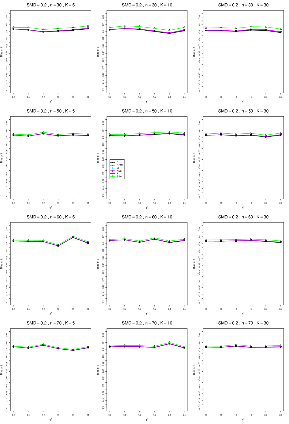
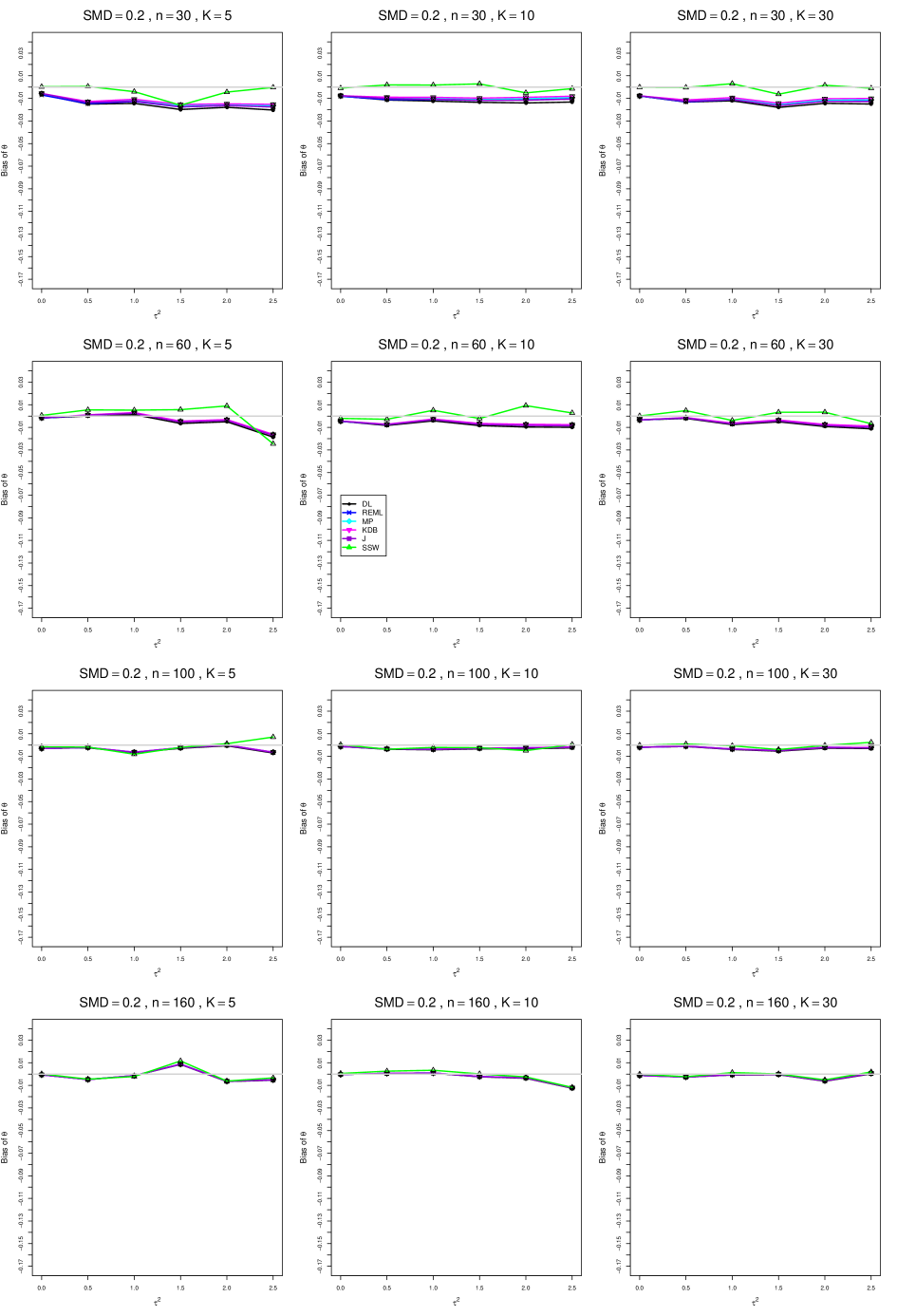
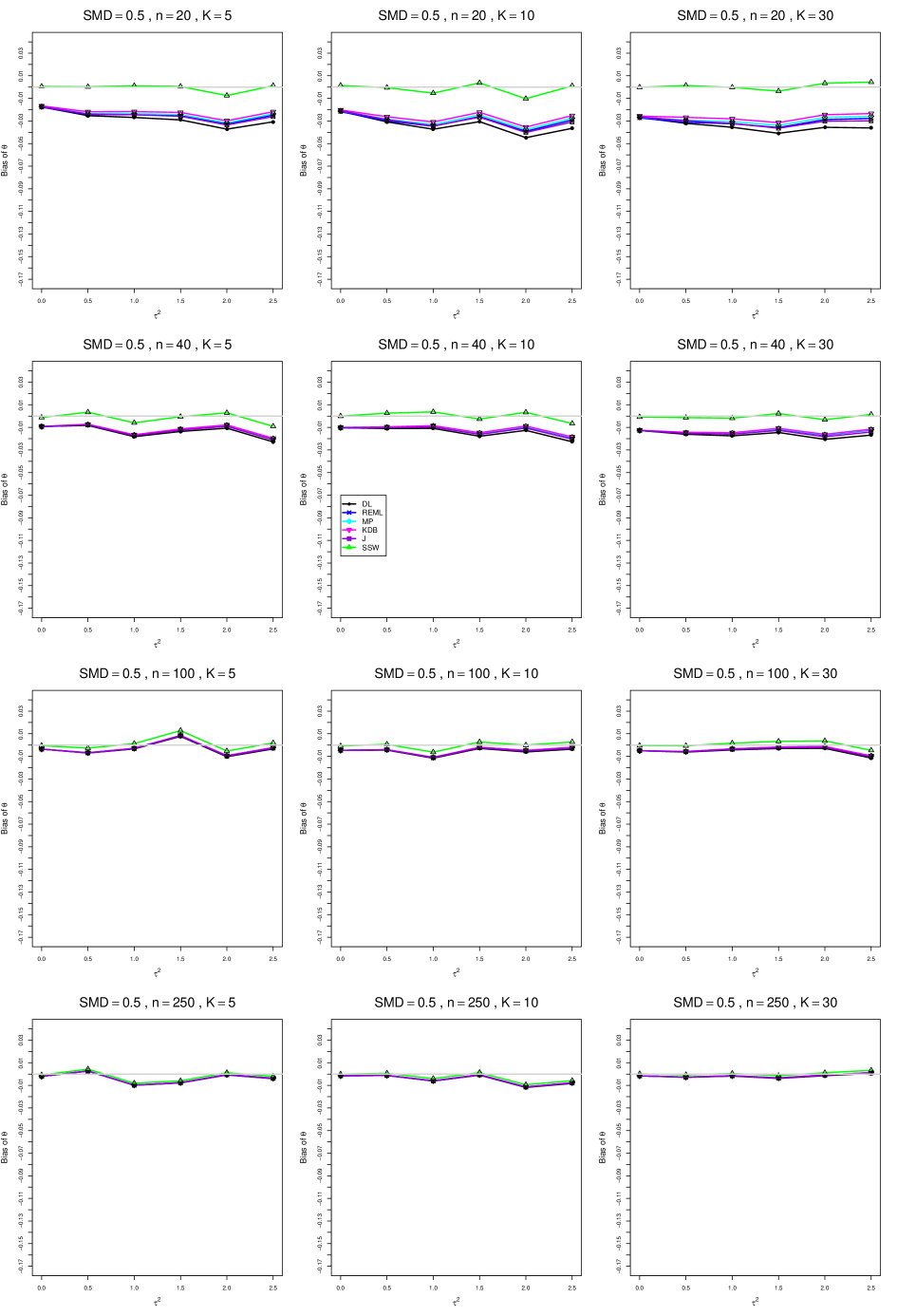
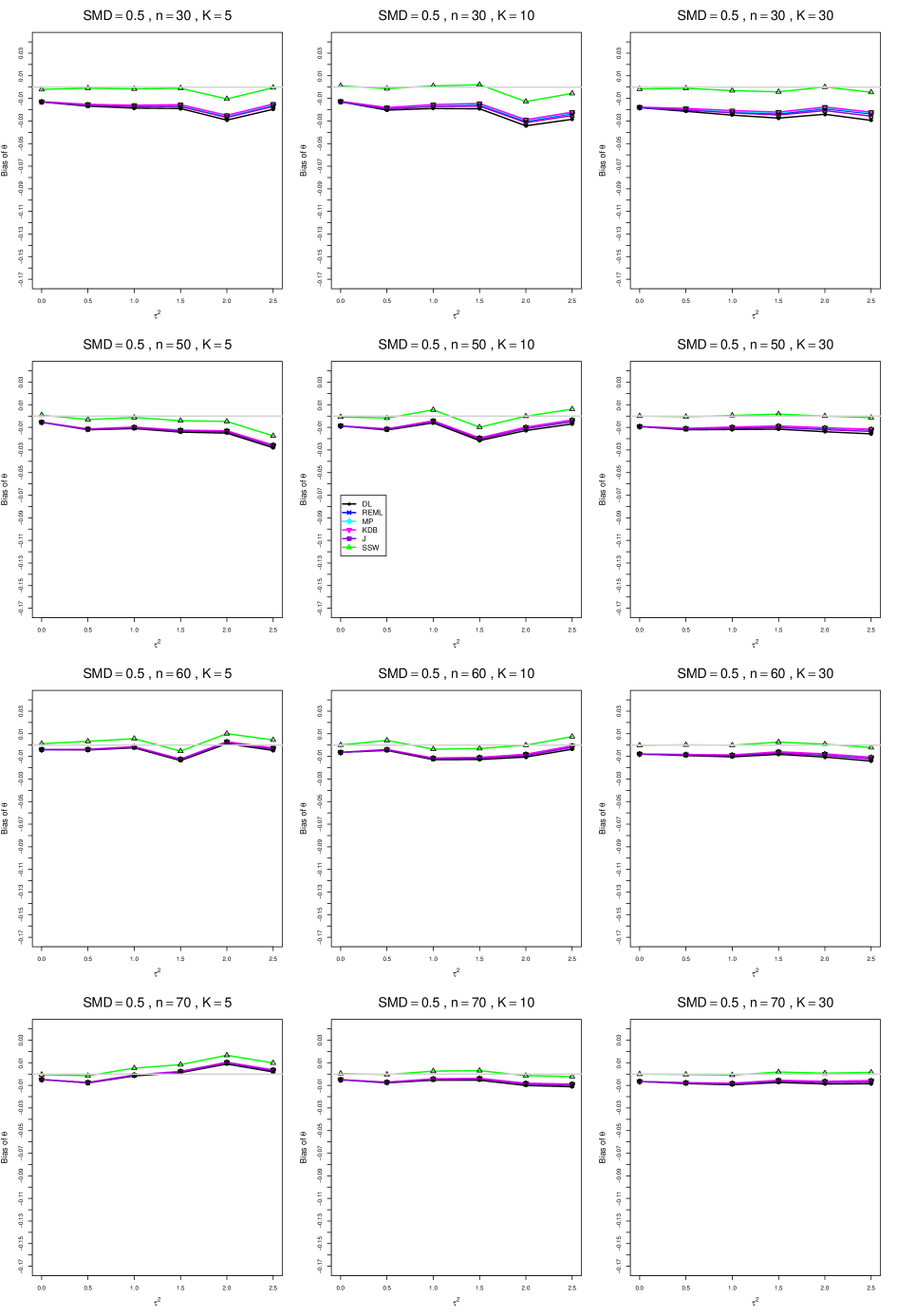
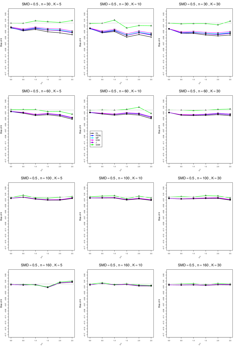
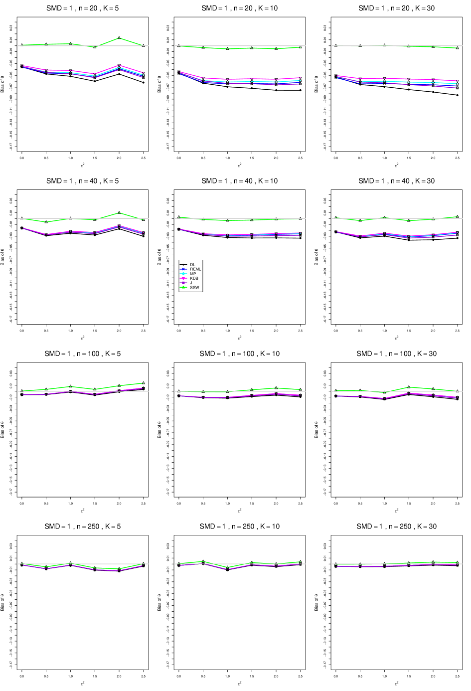
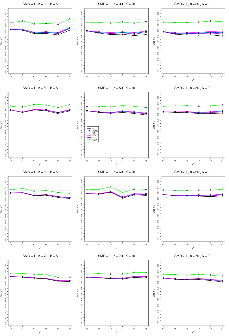
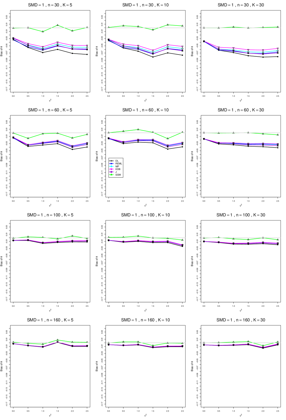
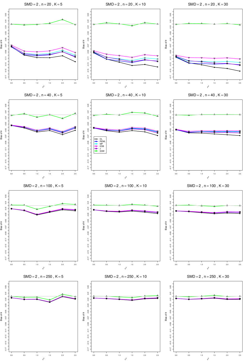
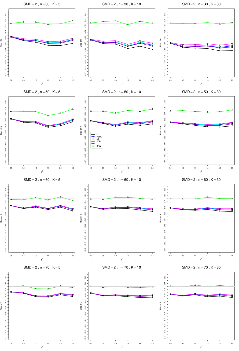
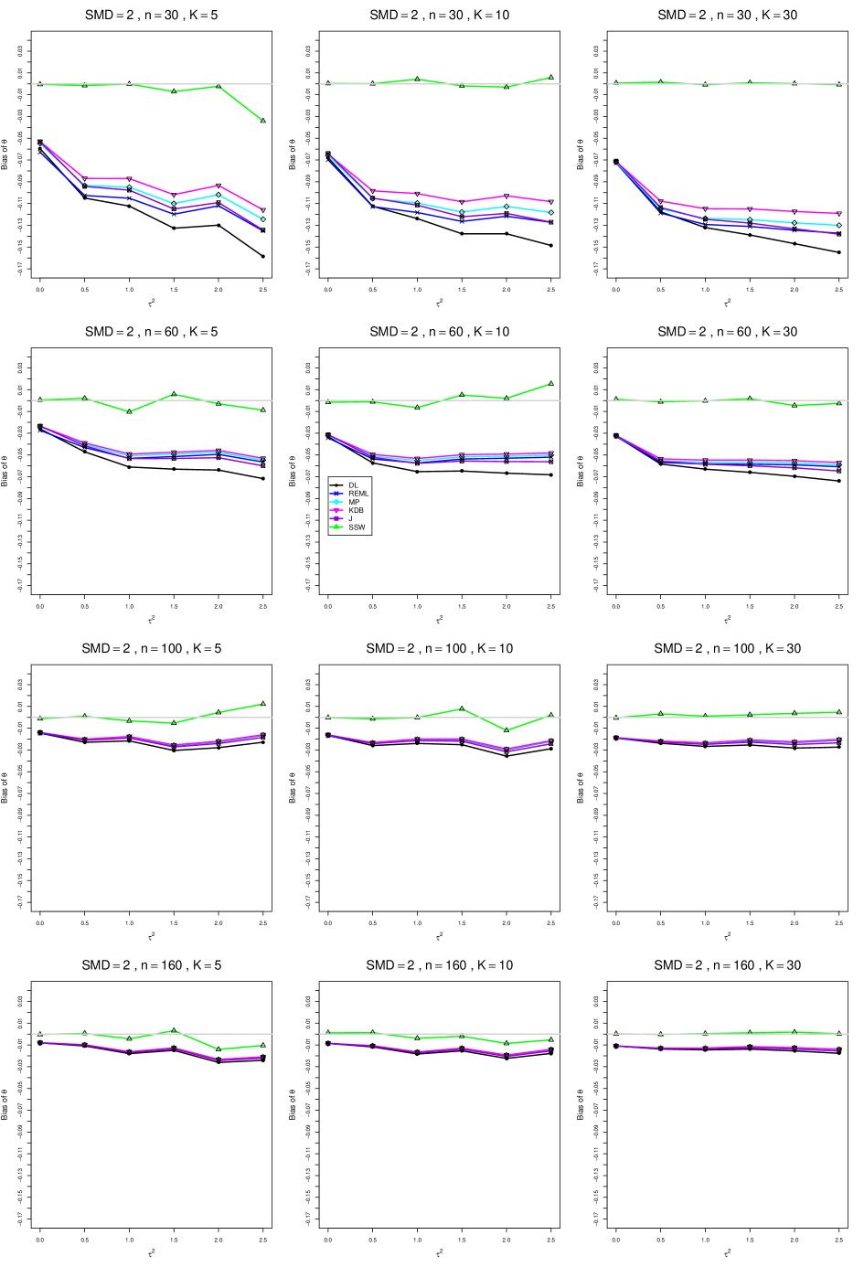
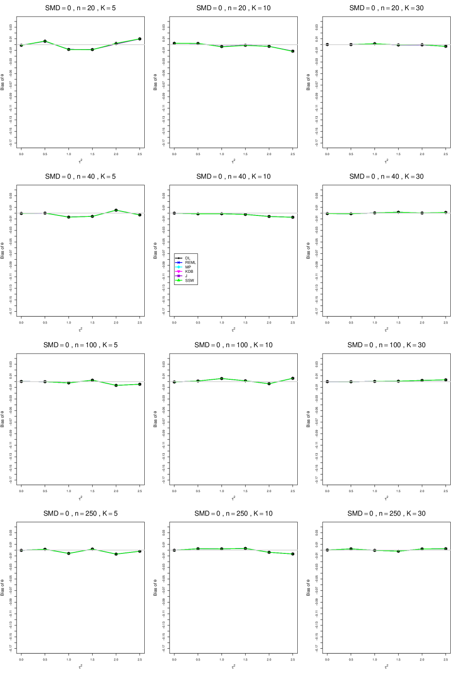
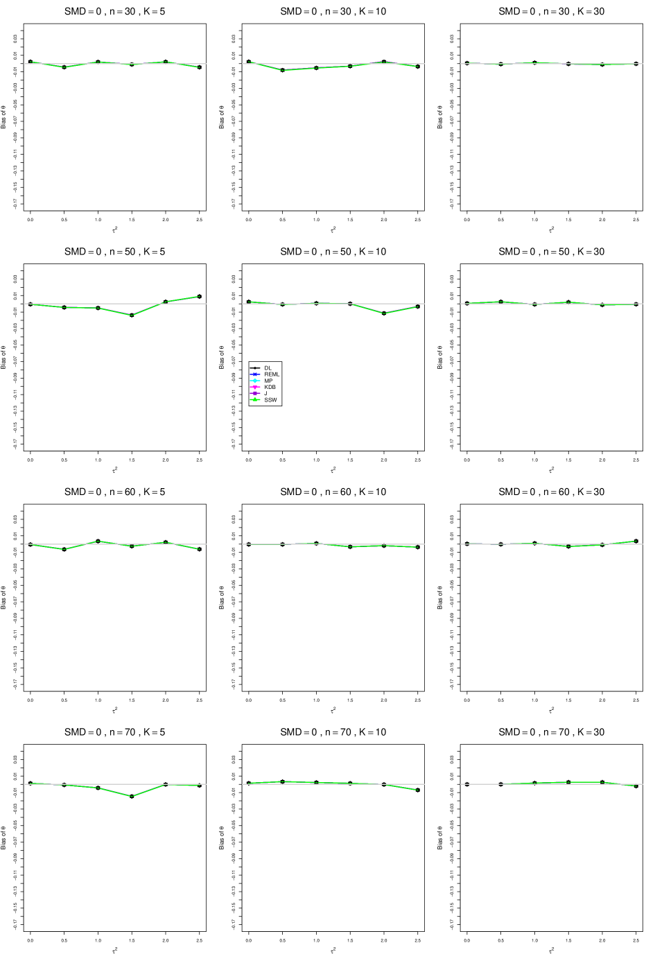
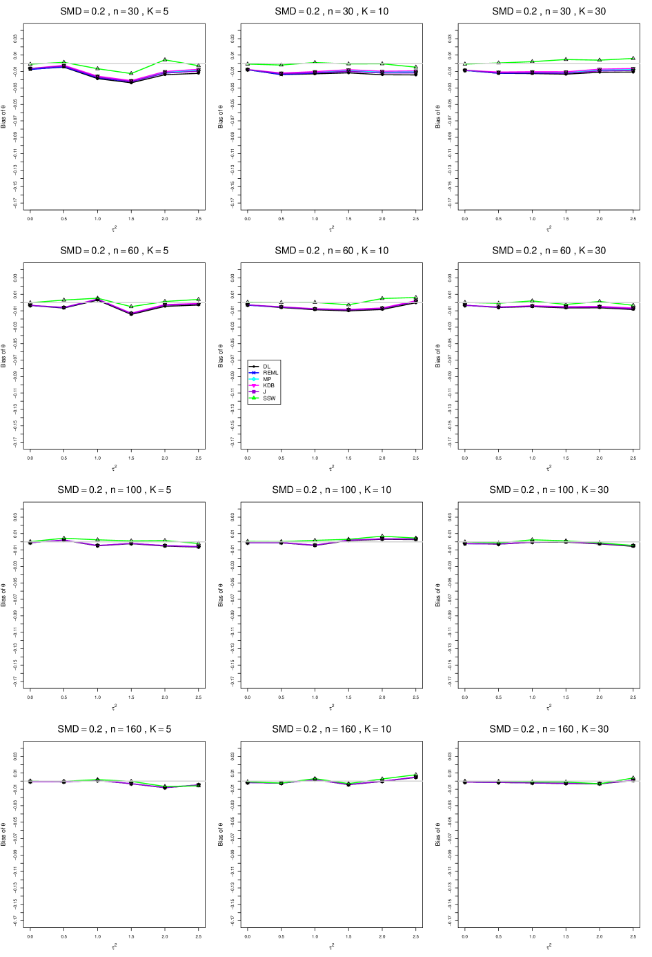
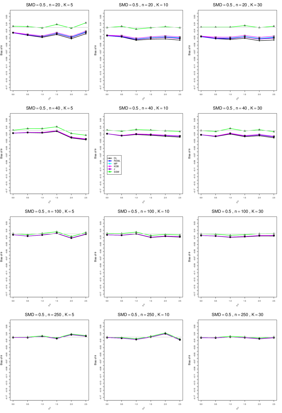
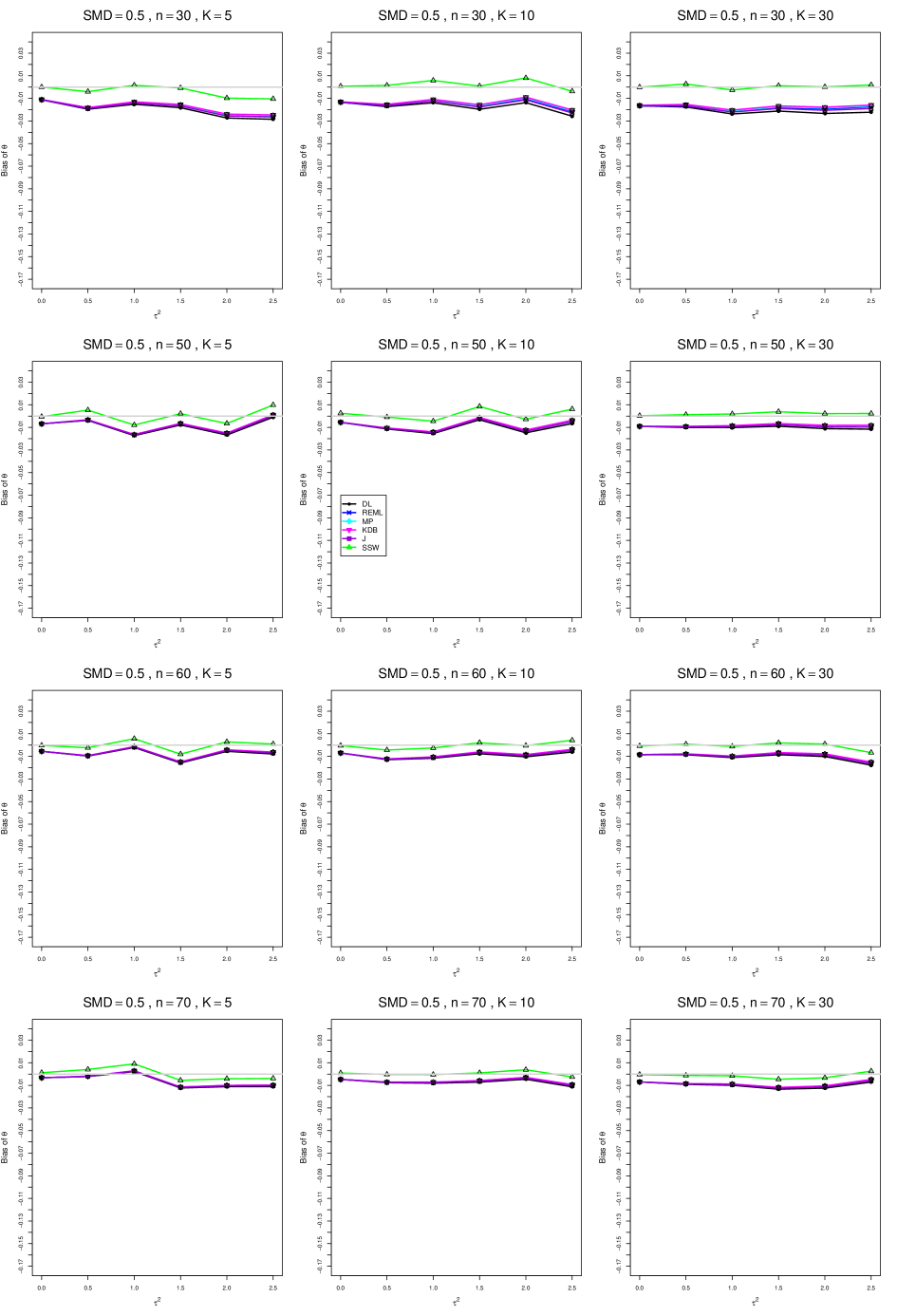
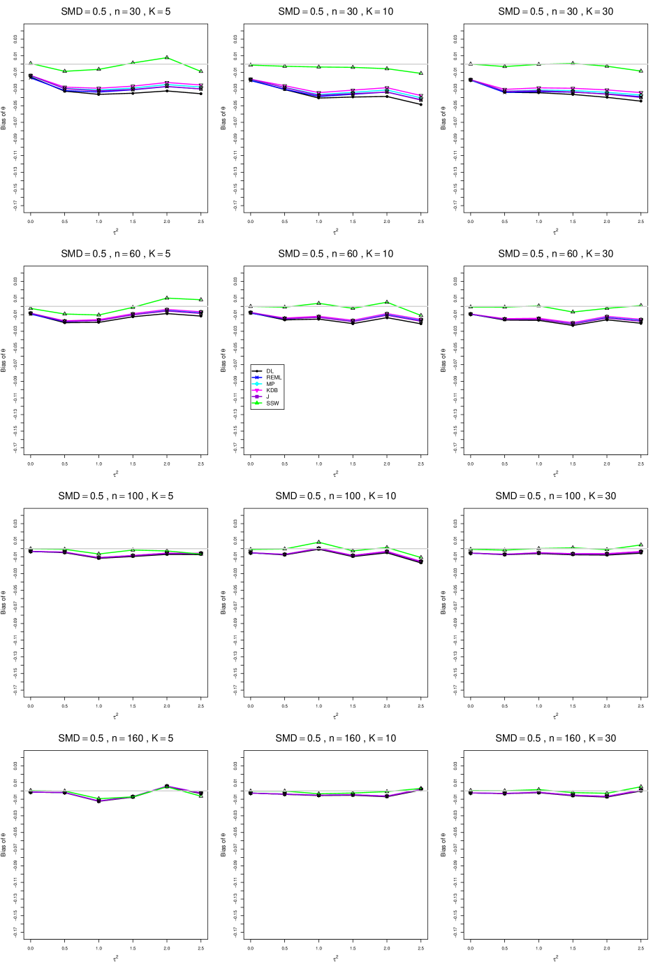
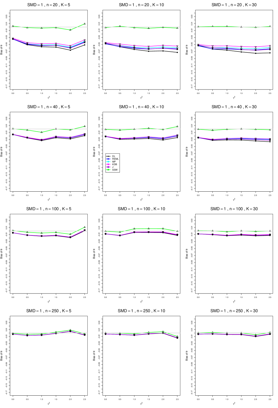
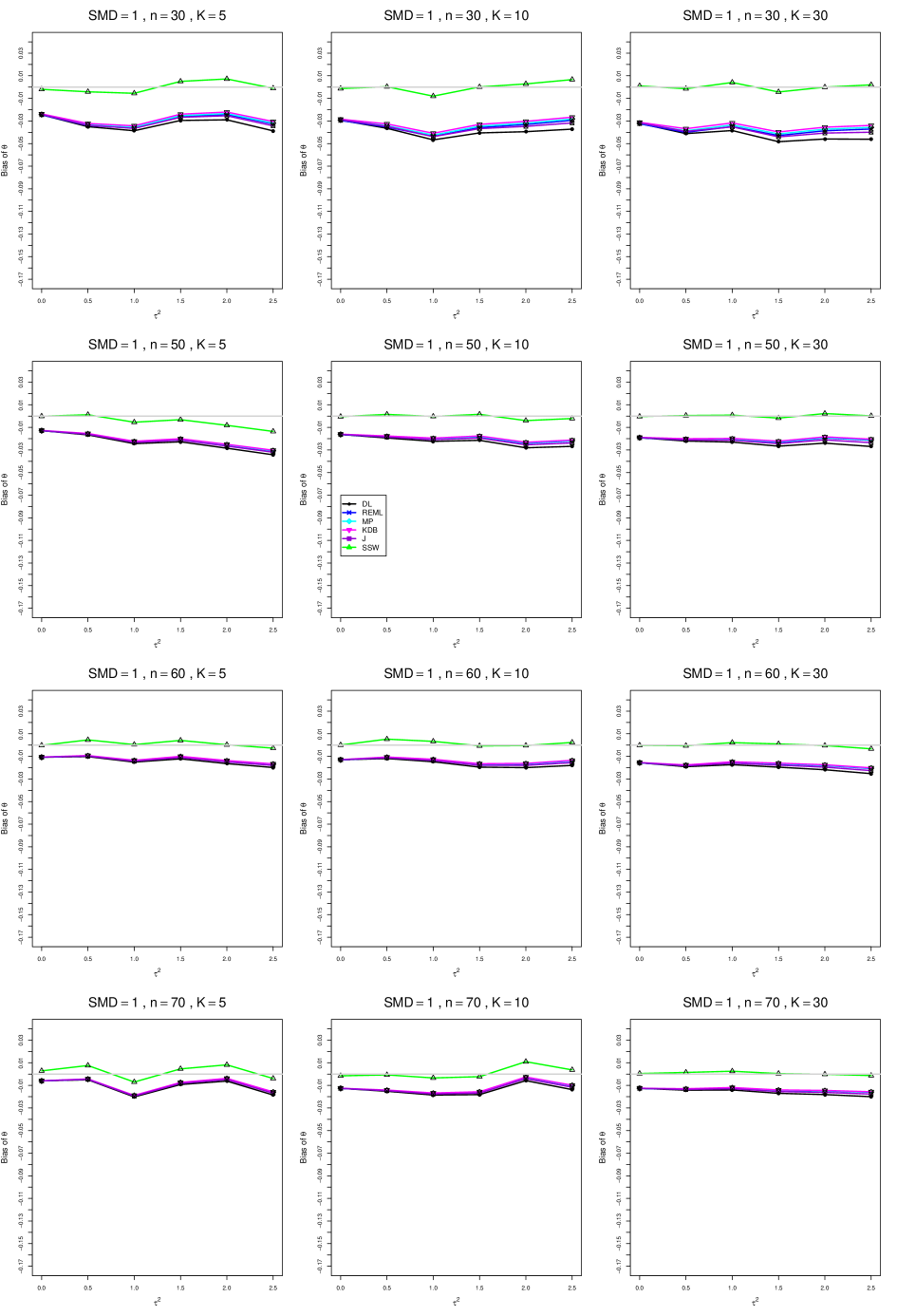
When , the bias of the six estimators (DL, REML, MP, KDB, J, and SSW) follows a single trace, close to 0, for all values of . When , SSW stays close to 0, and the others shift down, to increasingly negative bias, as increases, and their traces separate. For example, when , , , , and , the bias ranges from (KDB) to (DL), and MP, REML, and J (in that order) have intermediate values.
When , bias has little relation to . When , however, the bias of the estimators other than SSW (especially DL) becomes increasingly negative as increases. (The plot for and in B1.17 shows an extreme example.)
Where bias is nonzero, increasing or moves the traces toward (or to) 0, decreasing separation between them. Some plots (e.g., B1.37 and B1.39) show slight evidence of greater separation among traces when sample sizes are unequal and .
For the most part, has little or no effect on bias. Some plots suggest that, where bias is nonzero, separation among traces increases as increases, especially from to .
Bias does not differ noticeably between and .
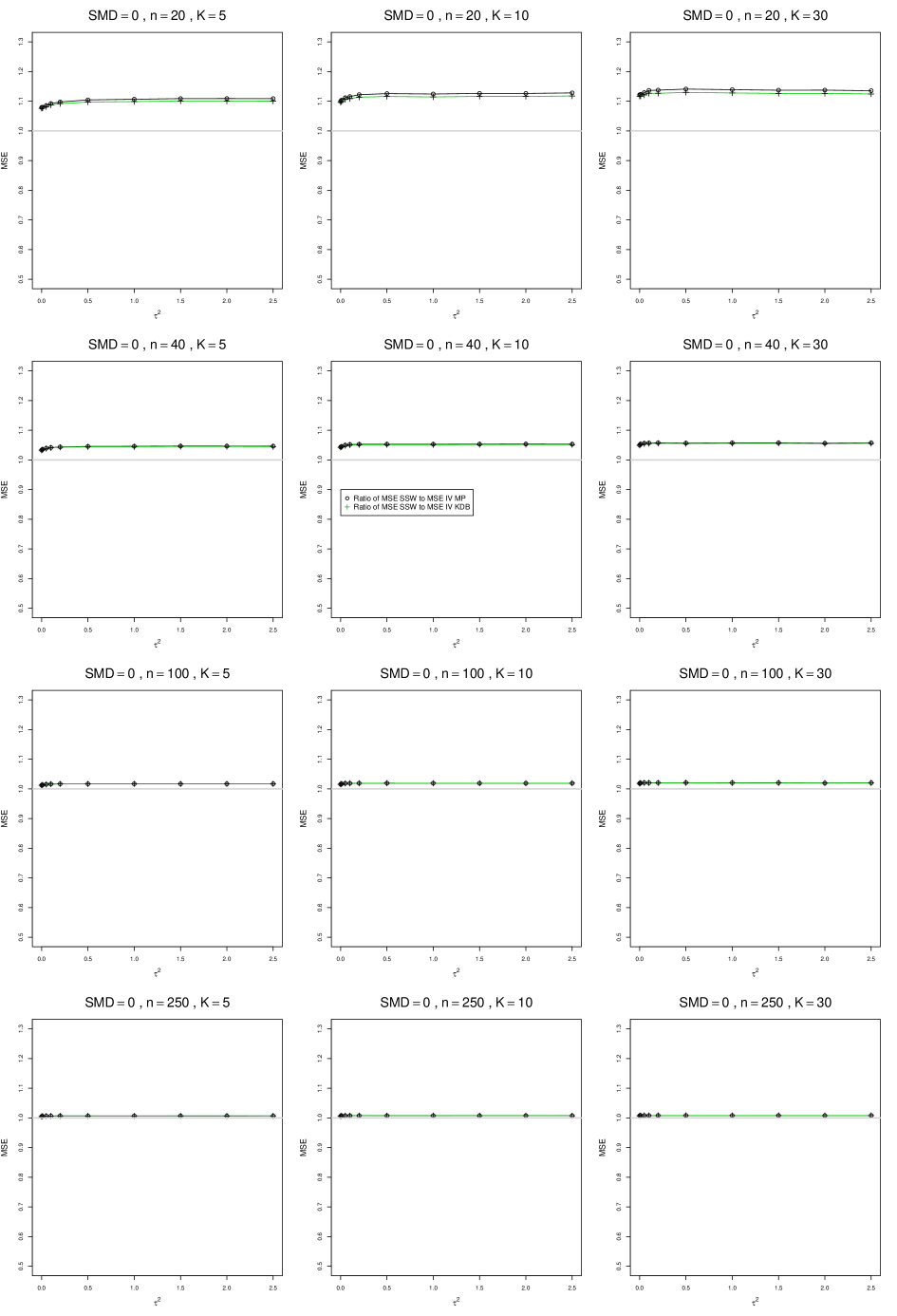
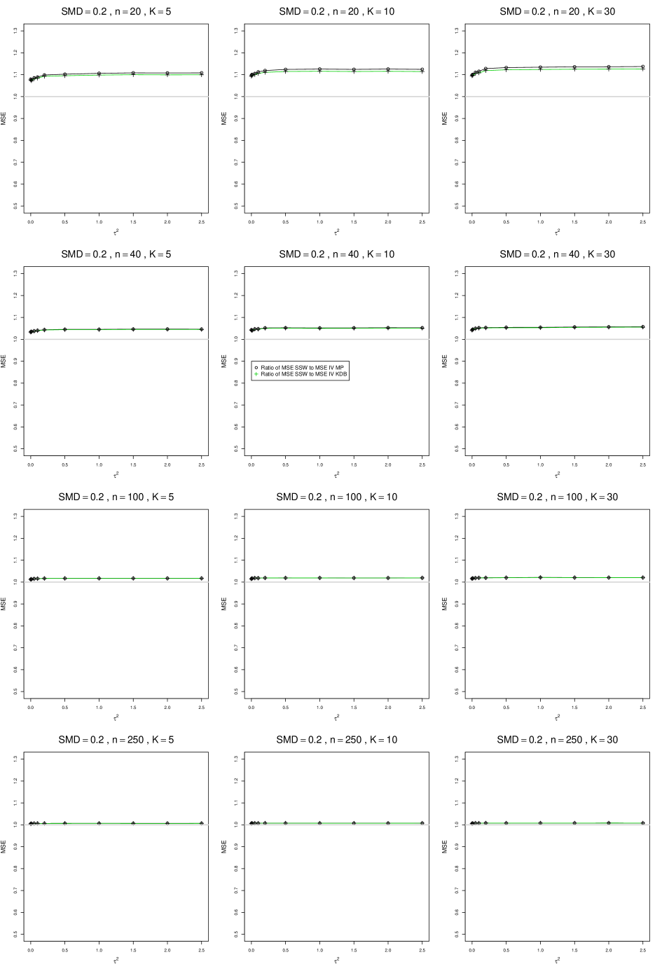
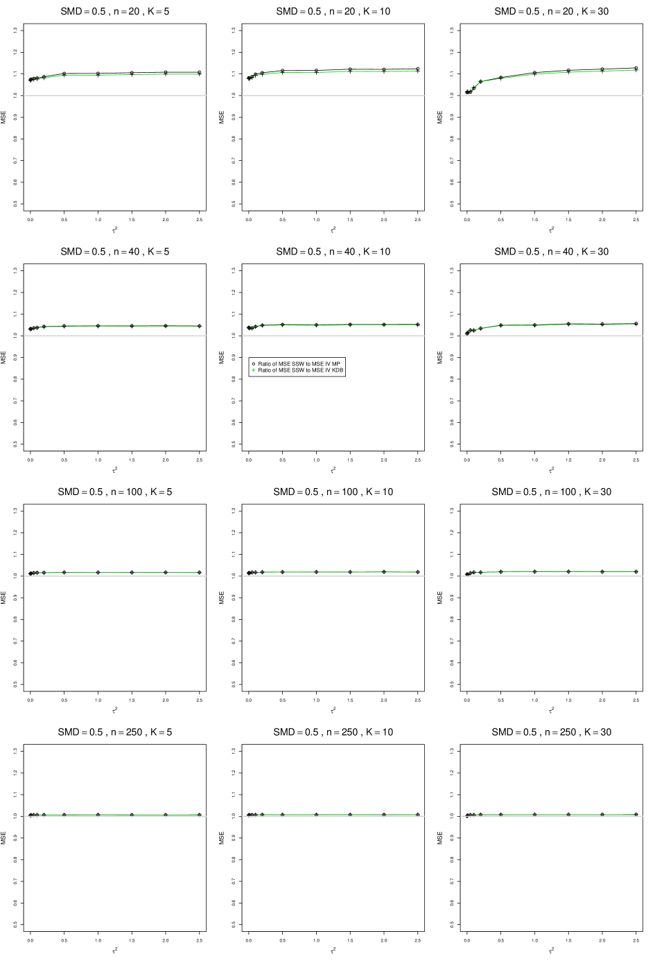
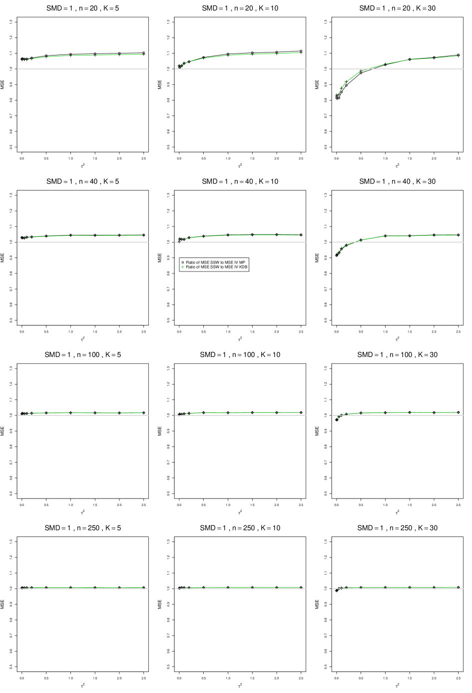
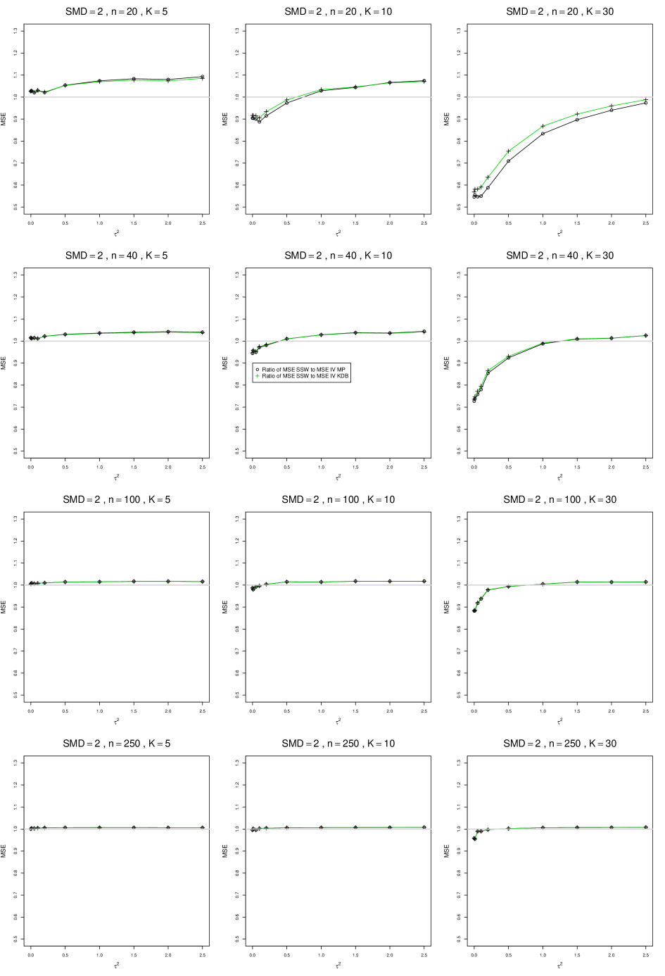
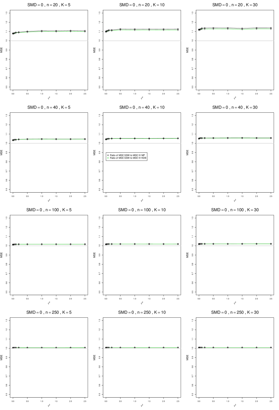
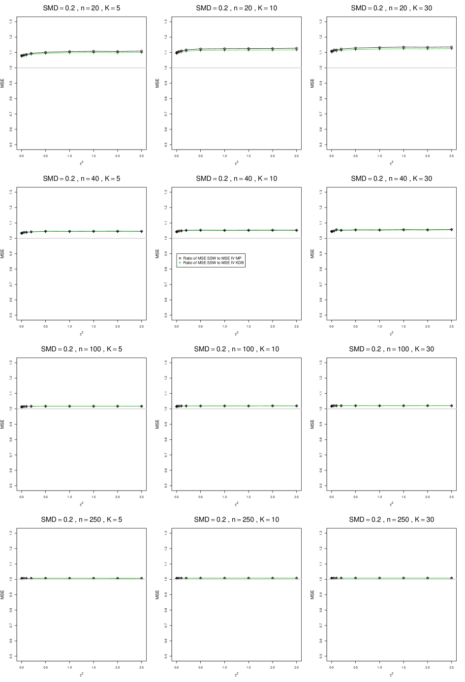
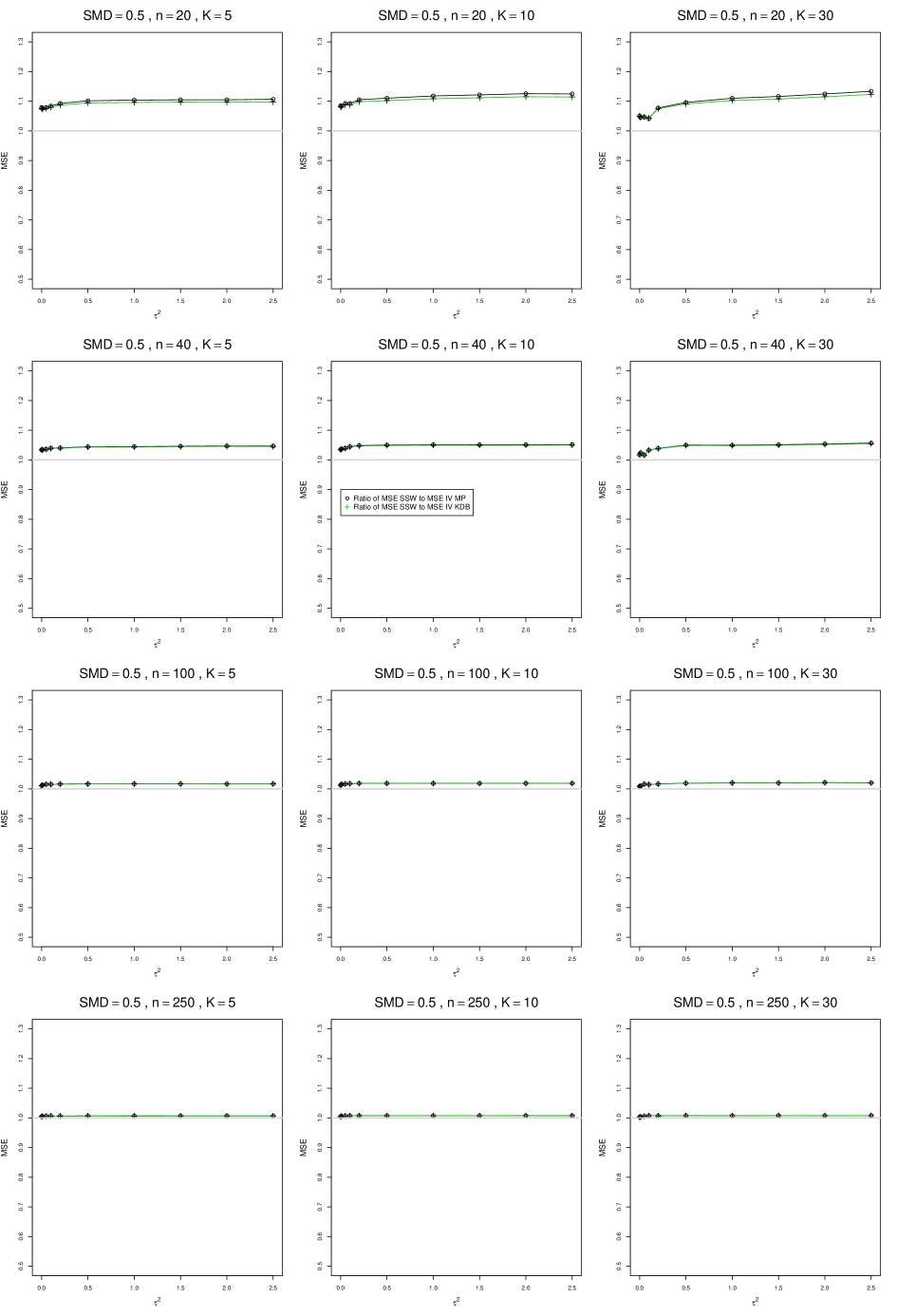
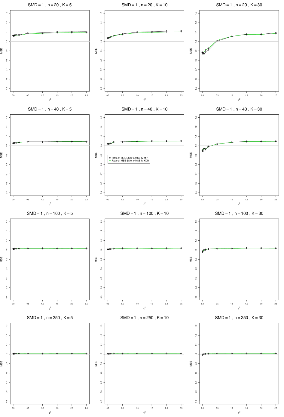
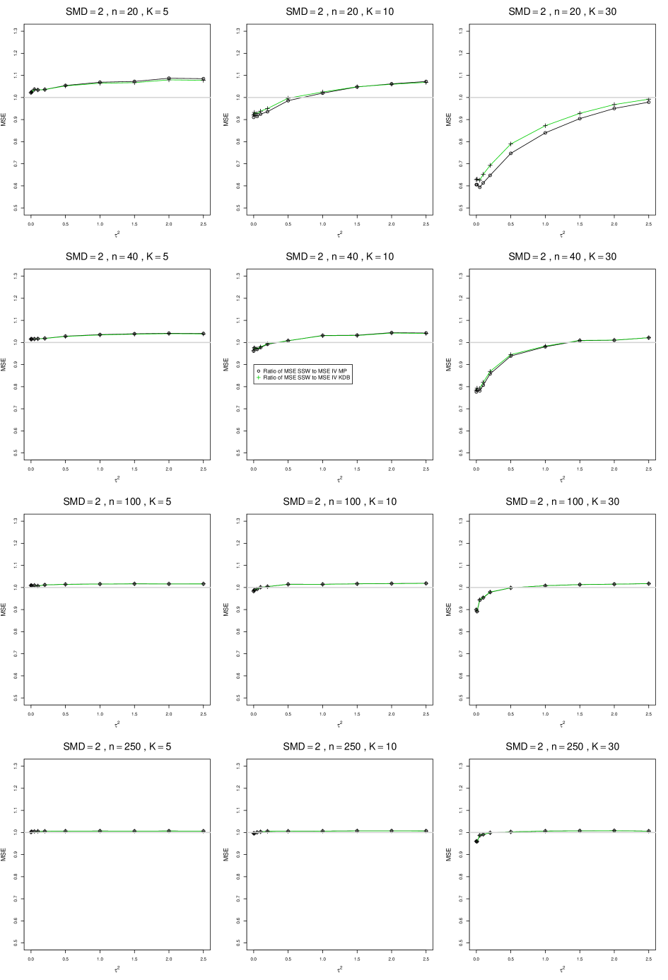
SSW essentially avoids the bias that we found in the inverse-variance-weighted estimators of . To provide an additional measure of its performance (besides coverage, discussed below). we estimated the mean squared error of SSW and the best two inverse-variance-weighted estimators, KDB and MP. Appendix E1 includes figures that plot (versus ) the ratios MSE(SSW)/MSE(KDB) and MSE(SSW)/MSE(MP) for the five values of , the two values of , and . For most situations the two ratios are essentially equal and differ little among values of and . In most situations the traces are essentially flat as increases; otherwise, they curve downward as approaches 0. As increases, the ratios approach 1. For example, when and , they decrease from around 1.1 when to nearly 1.0 when . As increases (), the ratios at small decrease. This pattern is first noticeable when and and ; and as increases, it becomes more pronounced at that combination of and and extends to larger (with ) and to and . When , , , and , the traces for the two ratios are separate and curve up from around 0.55 at to slightly when . The patterns are similar for .
In summary, the bias of SSW is close to 0, and the other five estimators (DL, REML, J, MP, and KDB), which use inverse-variance weights, have greater (and negative) bias, amounting to 5 – 10% when sample sizes are small and . This bias increases as increases. SSW usually has slightly greater mean squared error than KDB and MP when is small, but its MSE can be substantially smaller, especially for small .
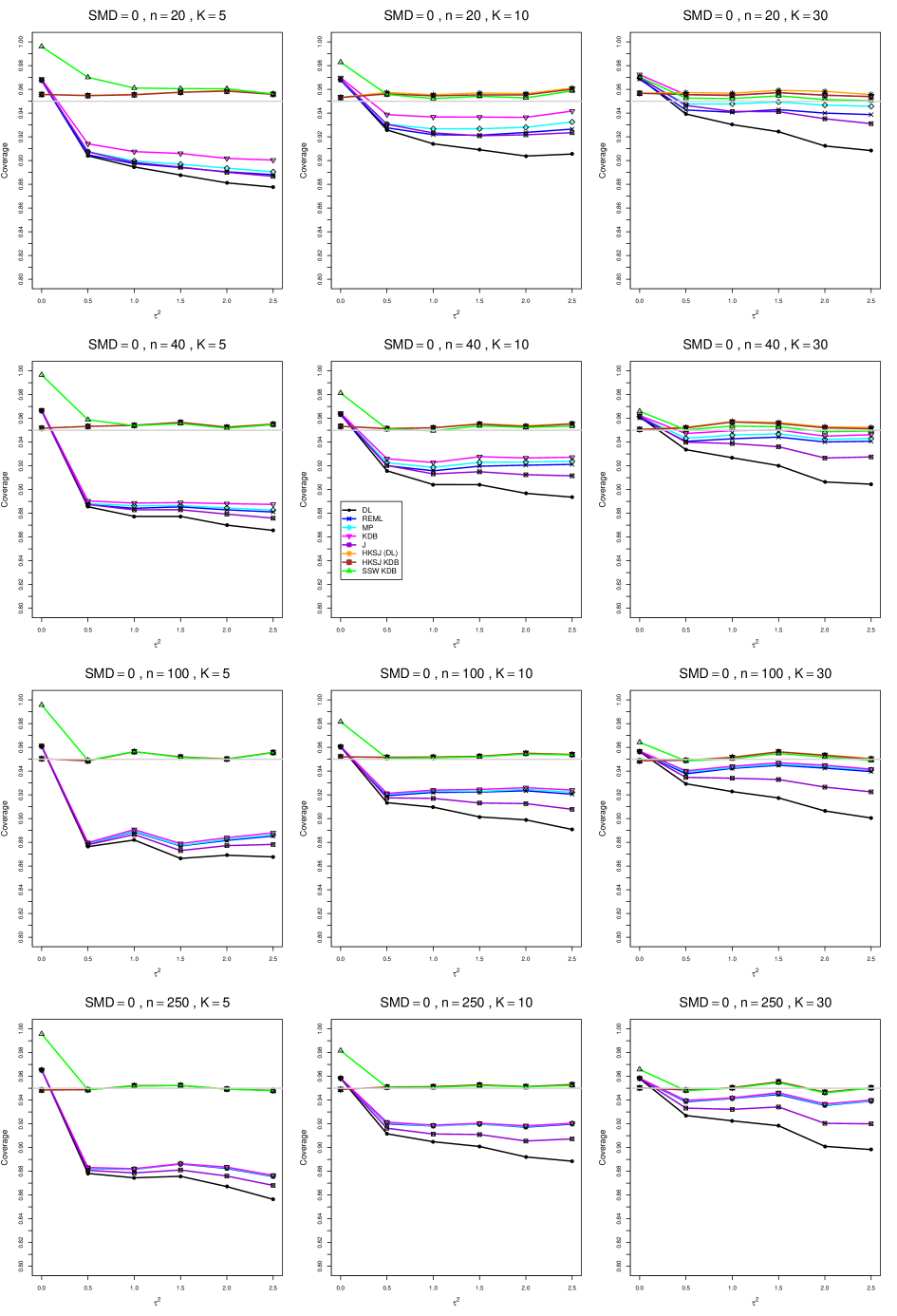
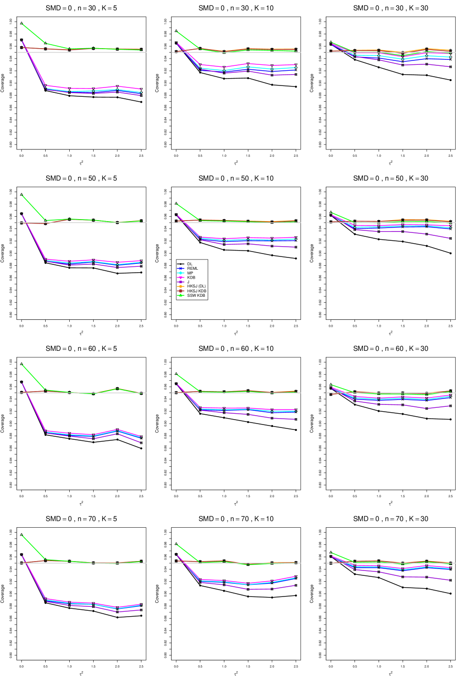
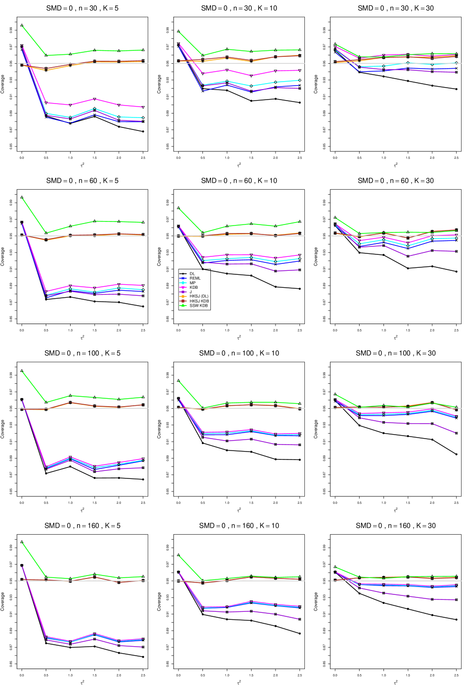
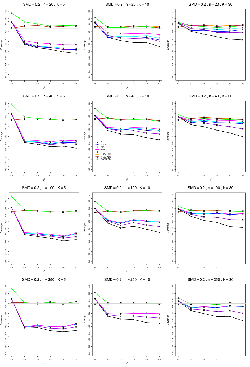
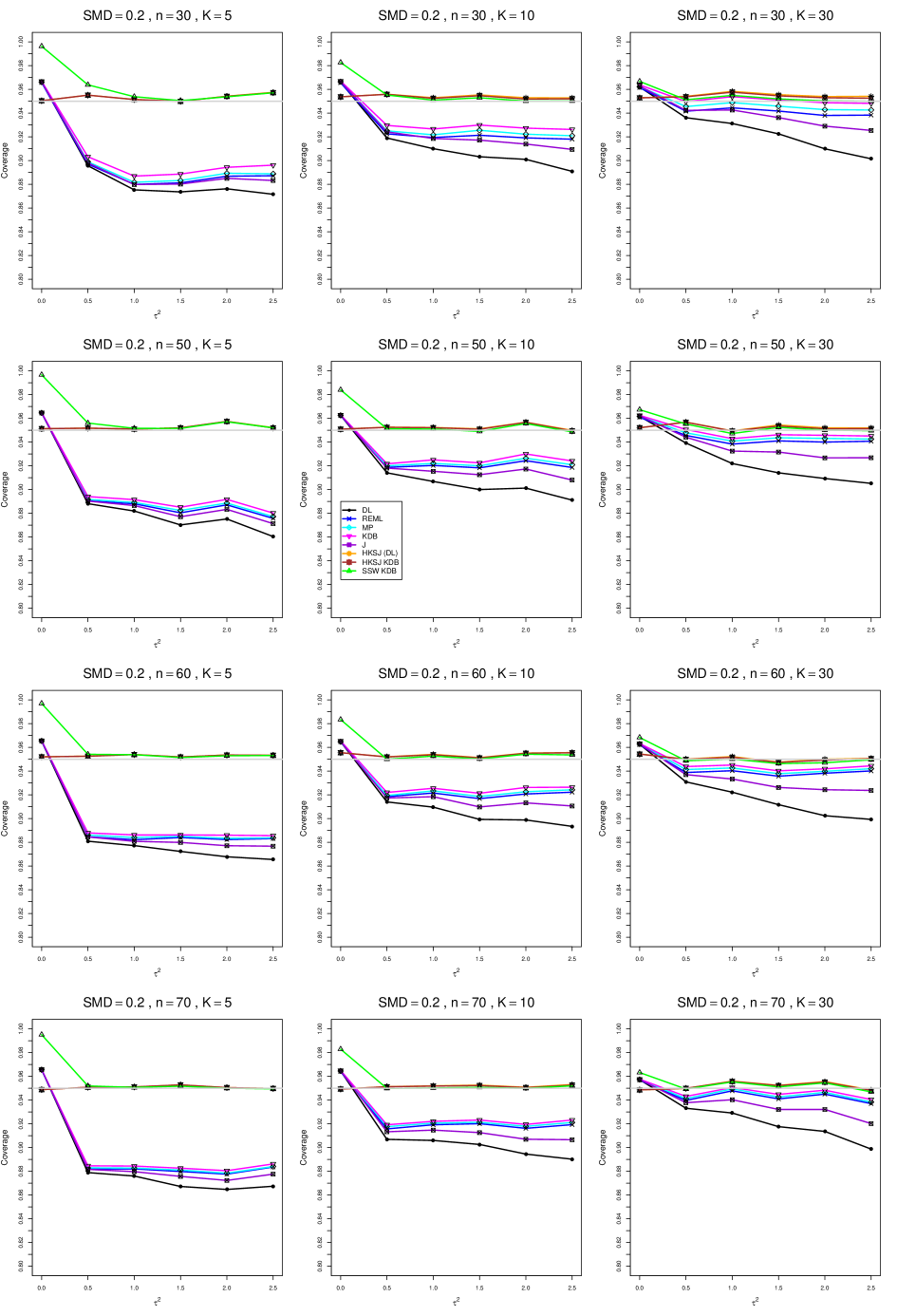
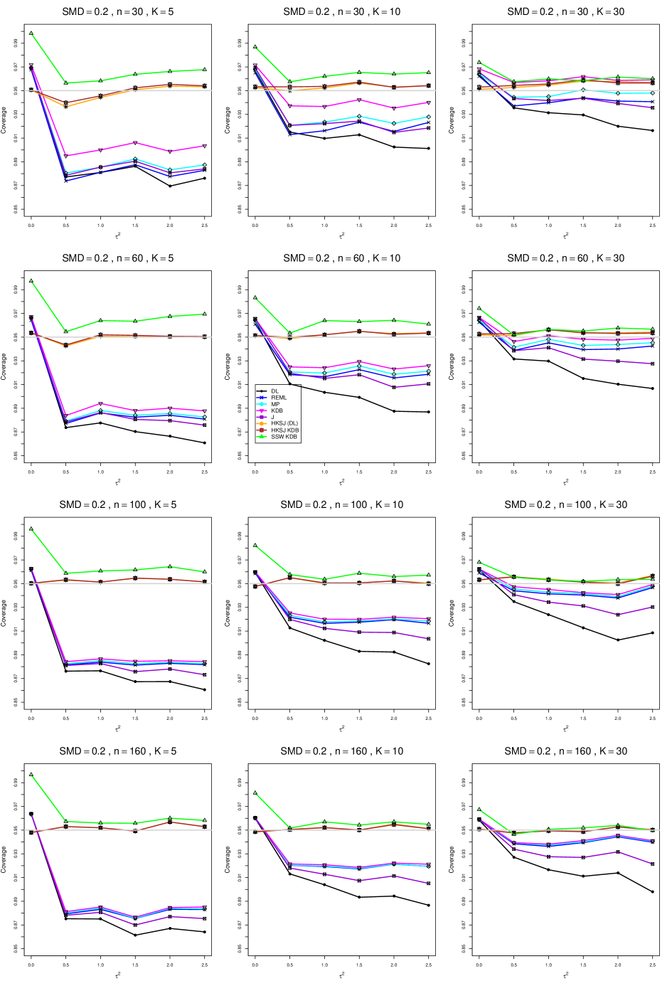
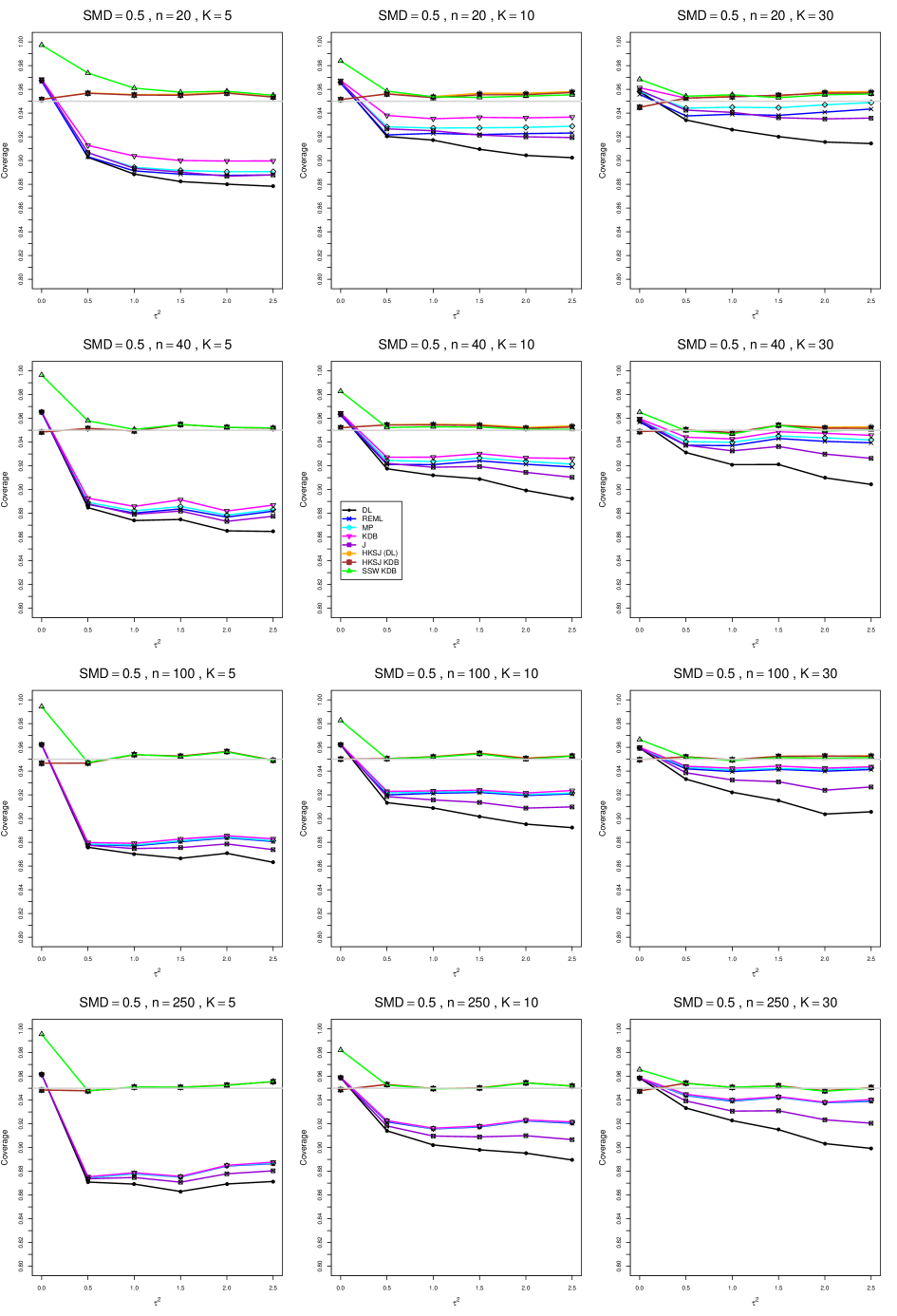
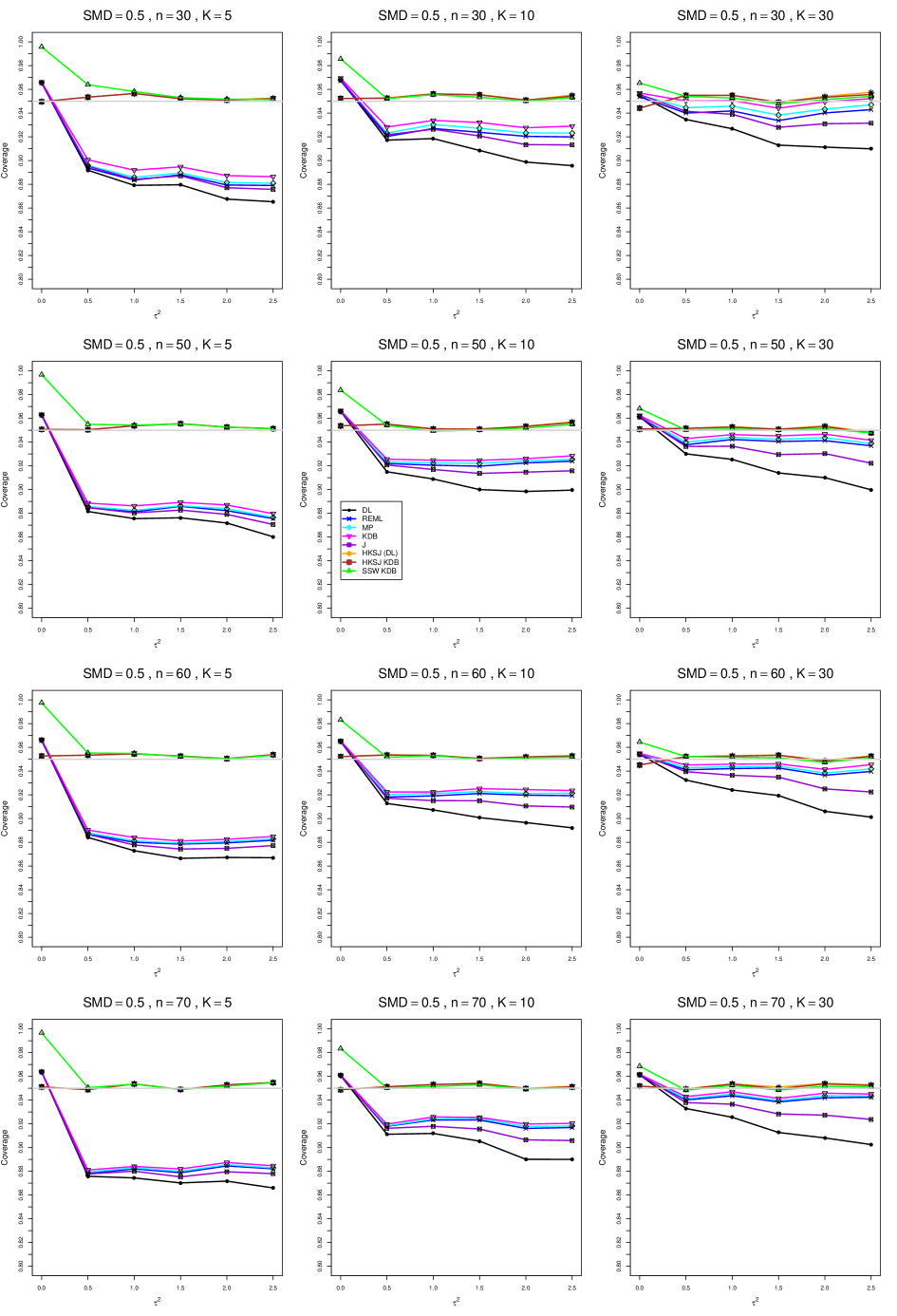
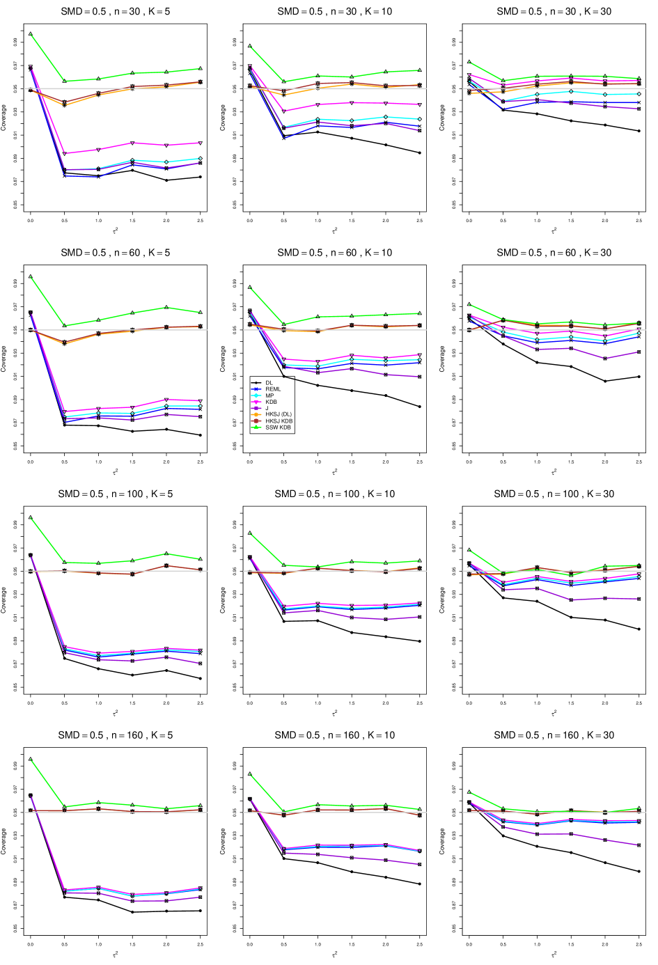
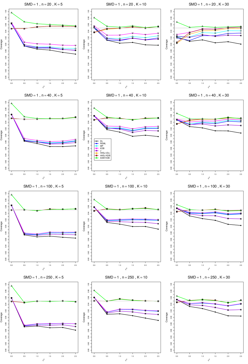
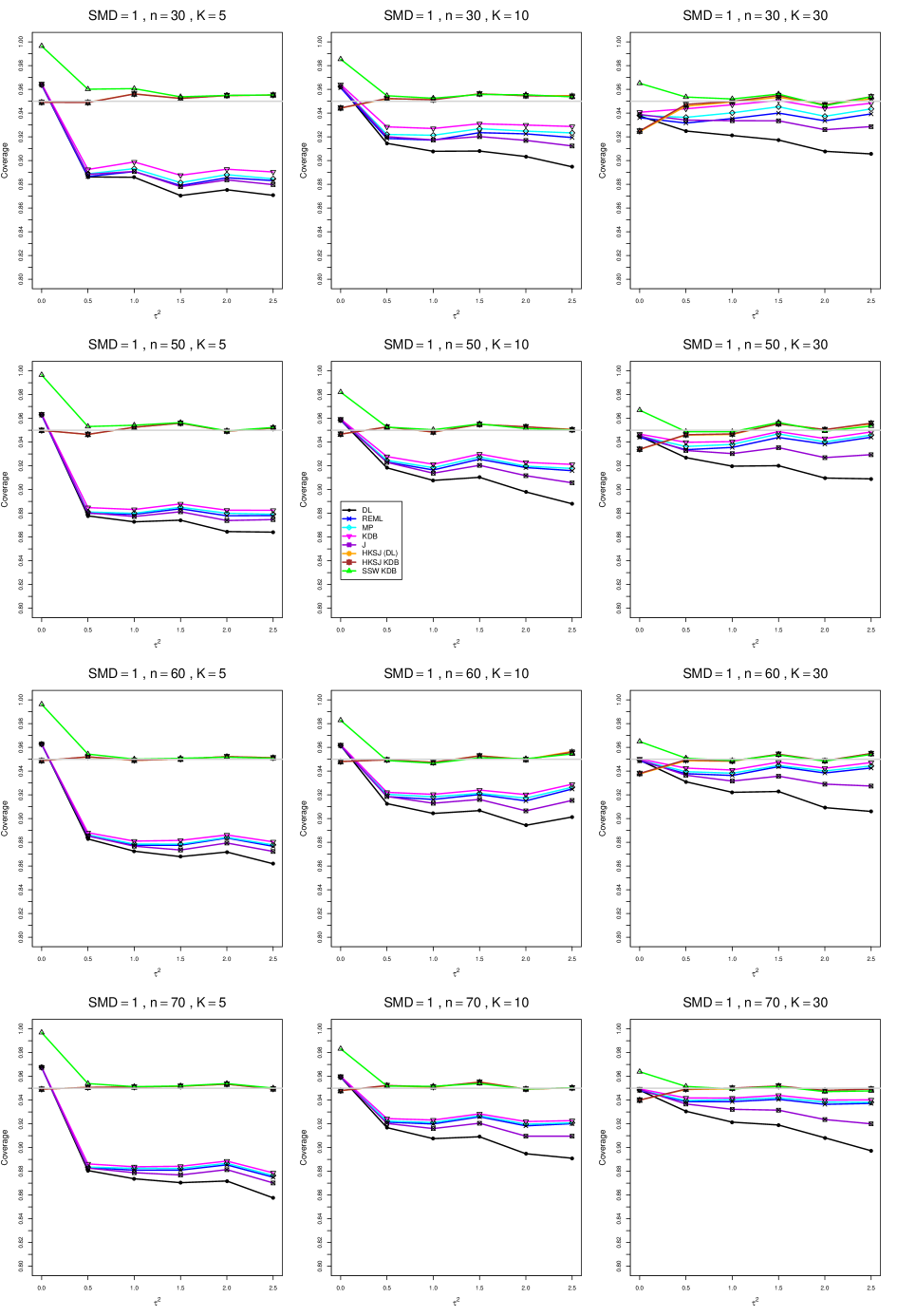
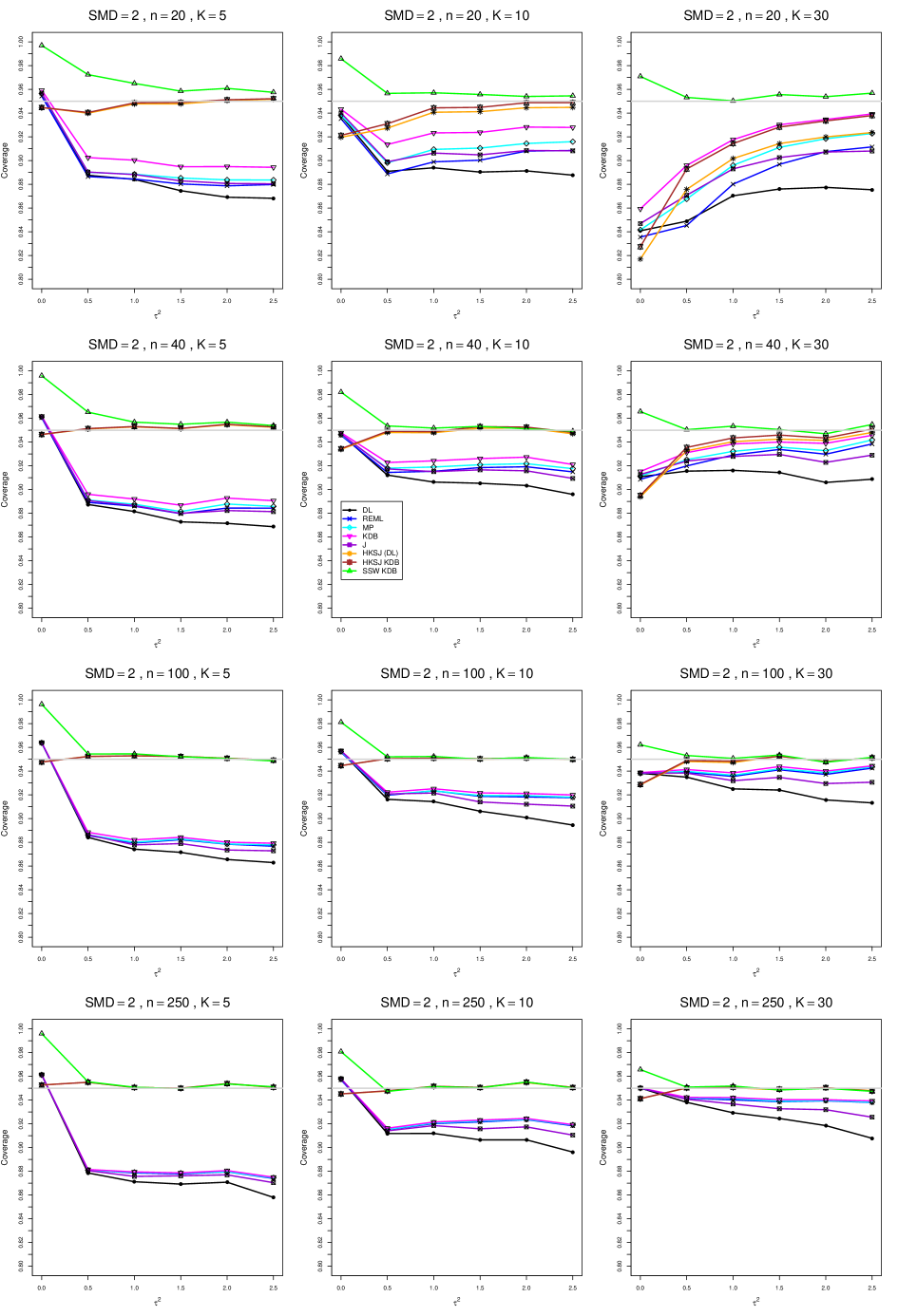
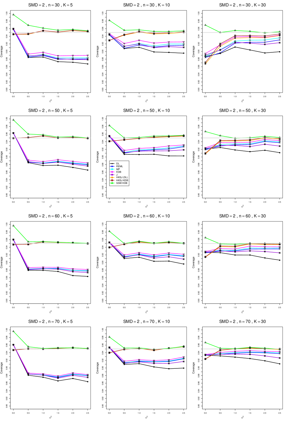
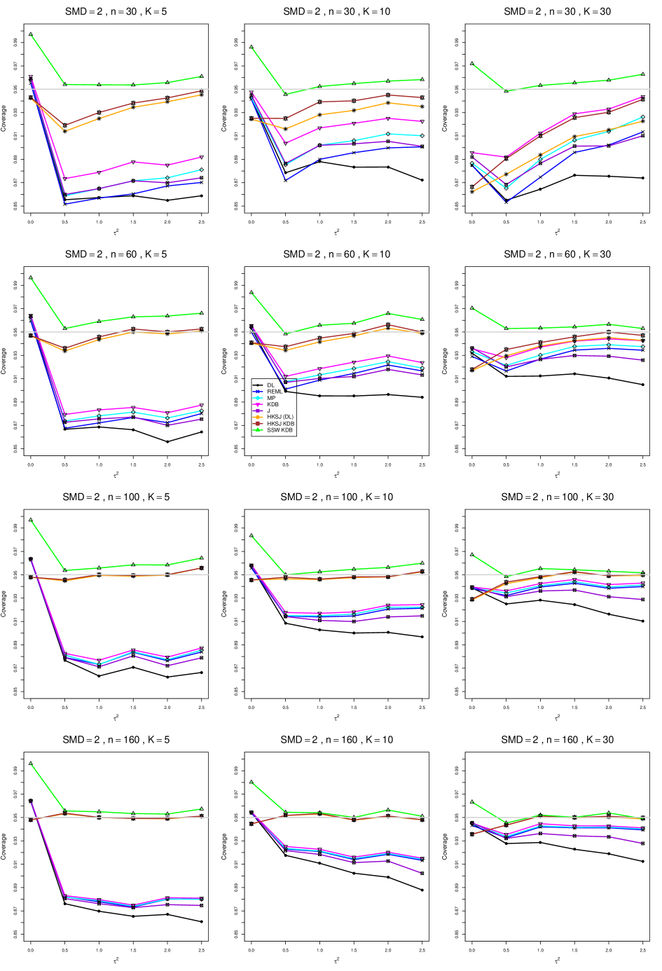
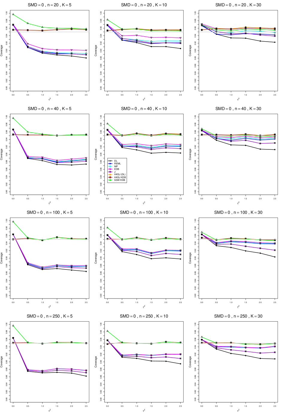
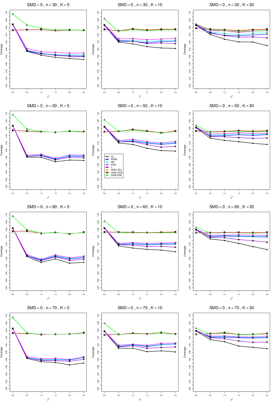
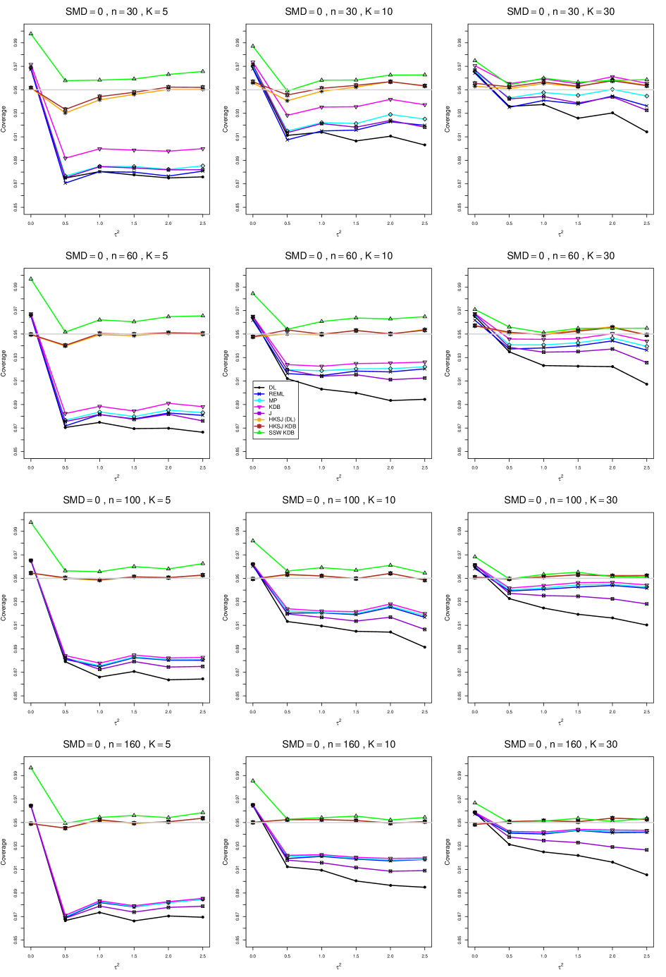
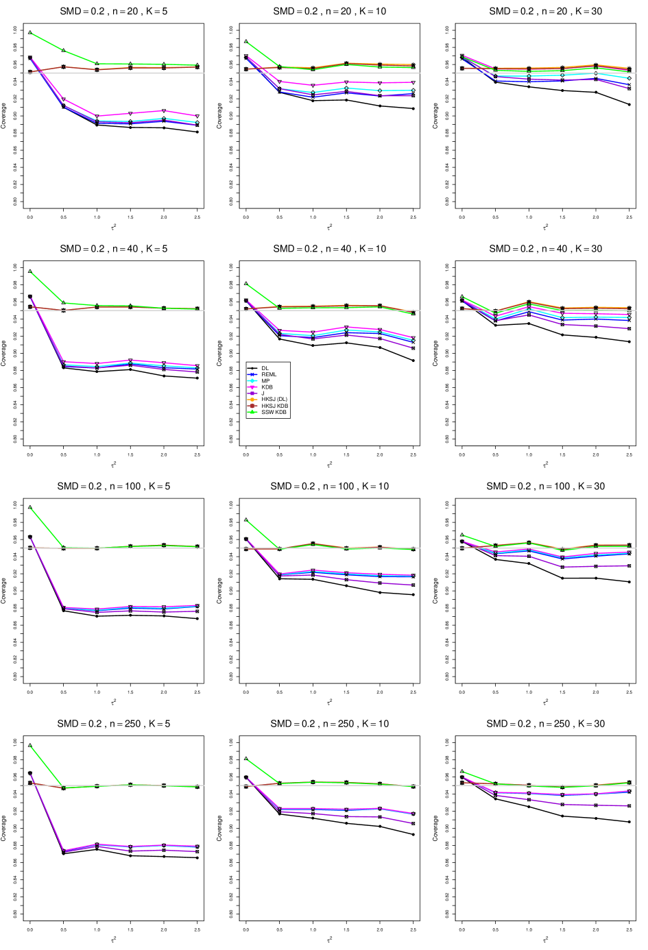
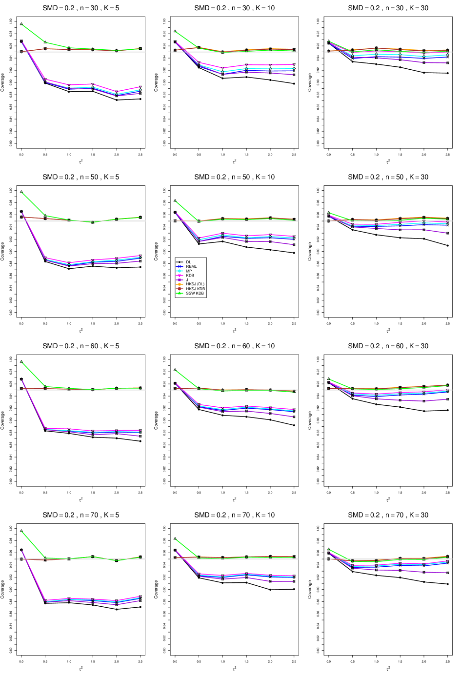
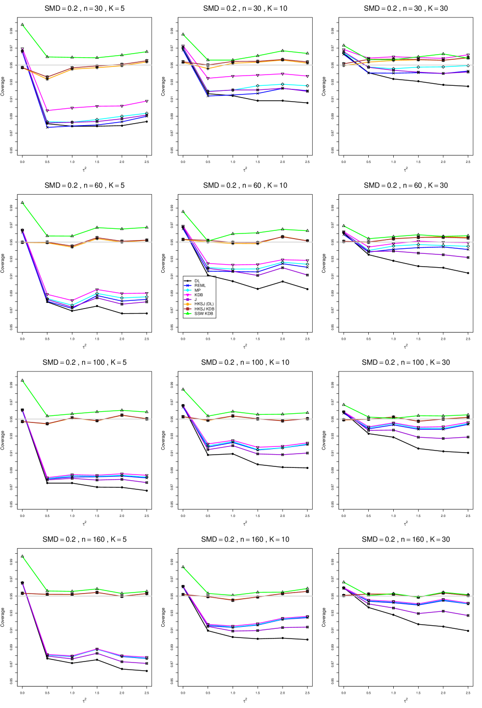
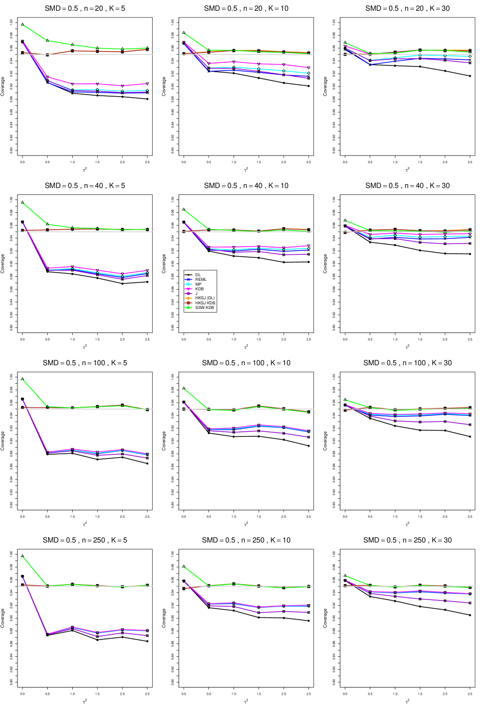
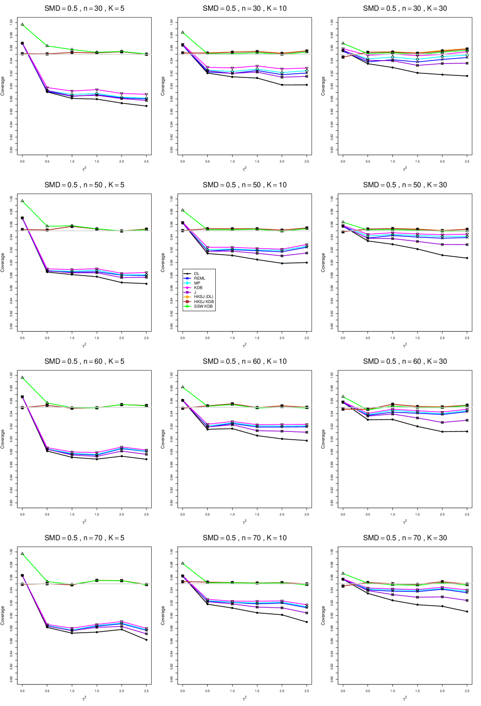
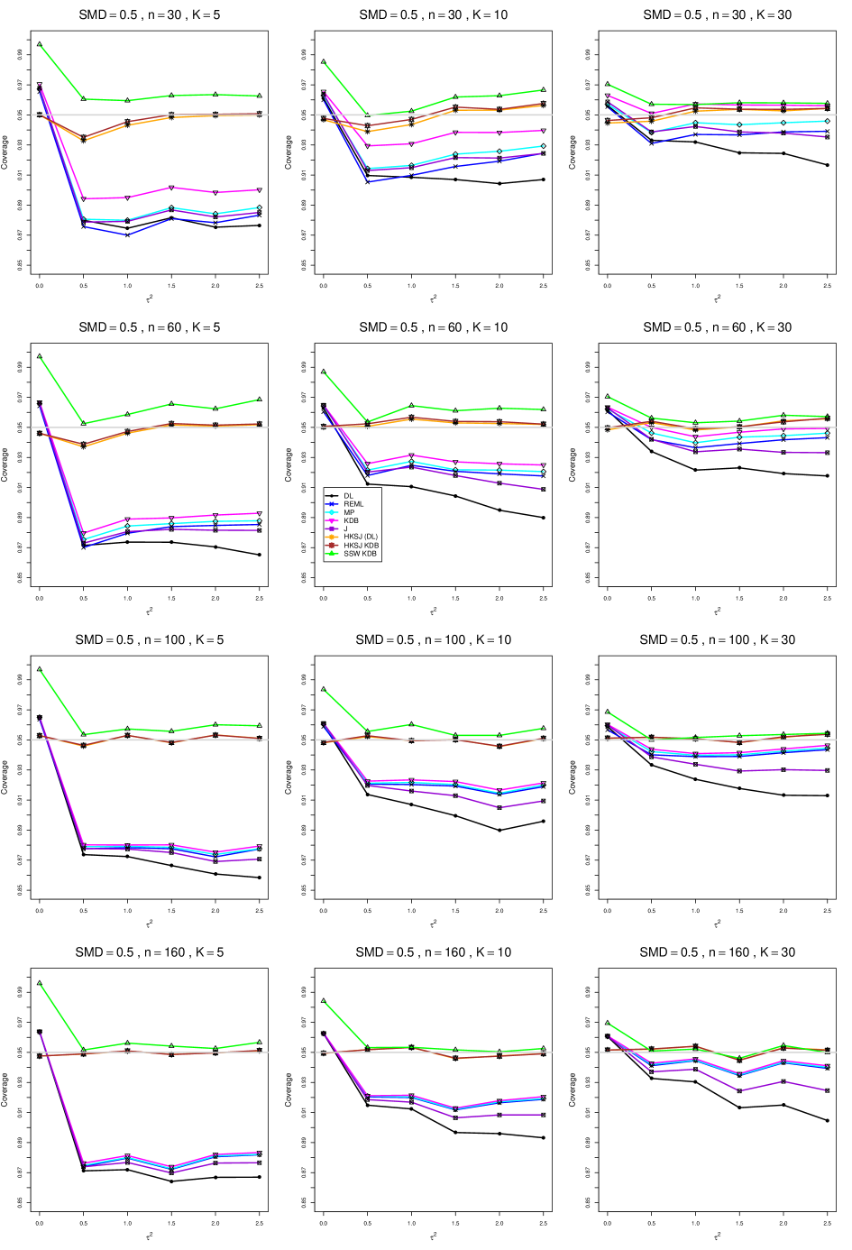
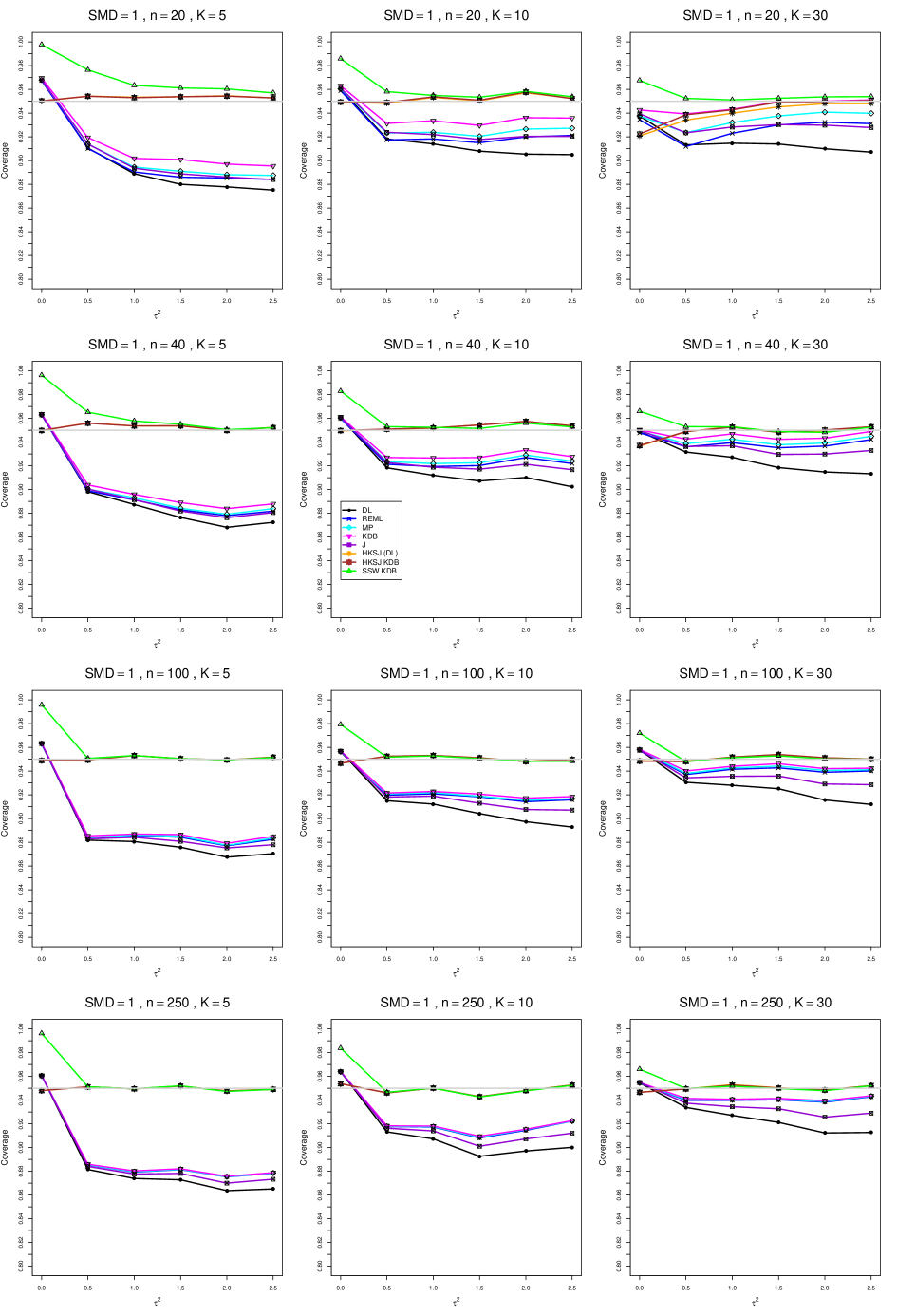
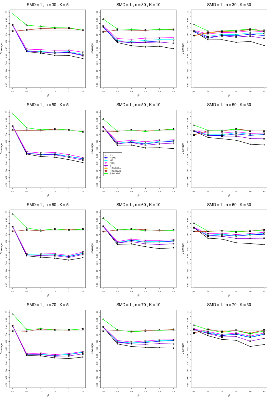
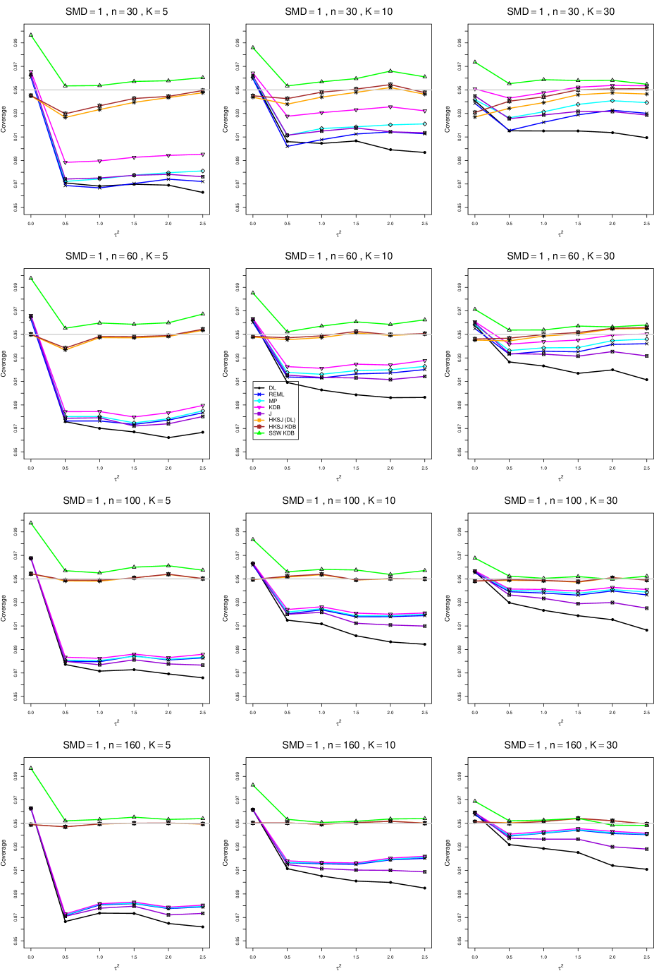
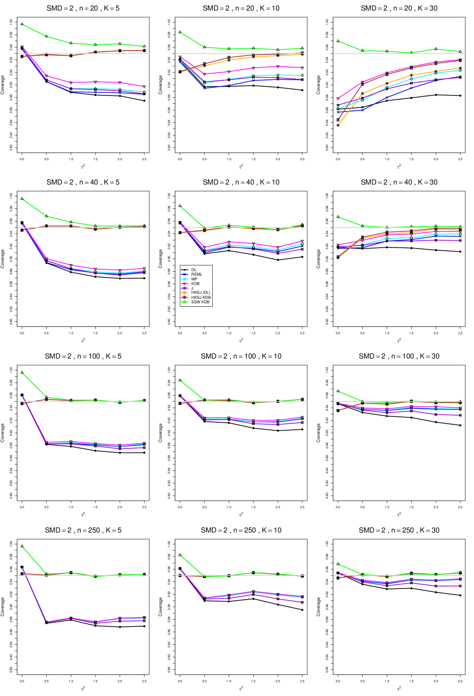
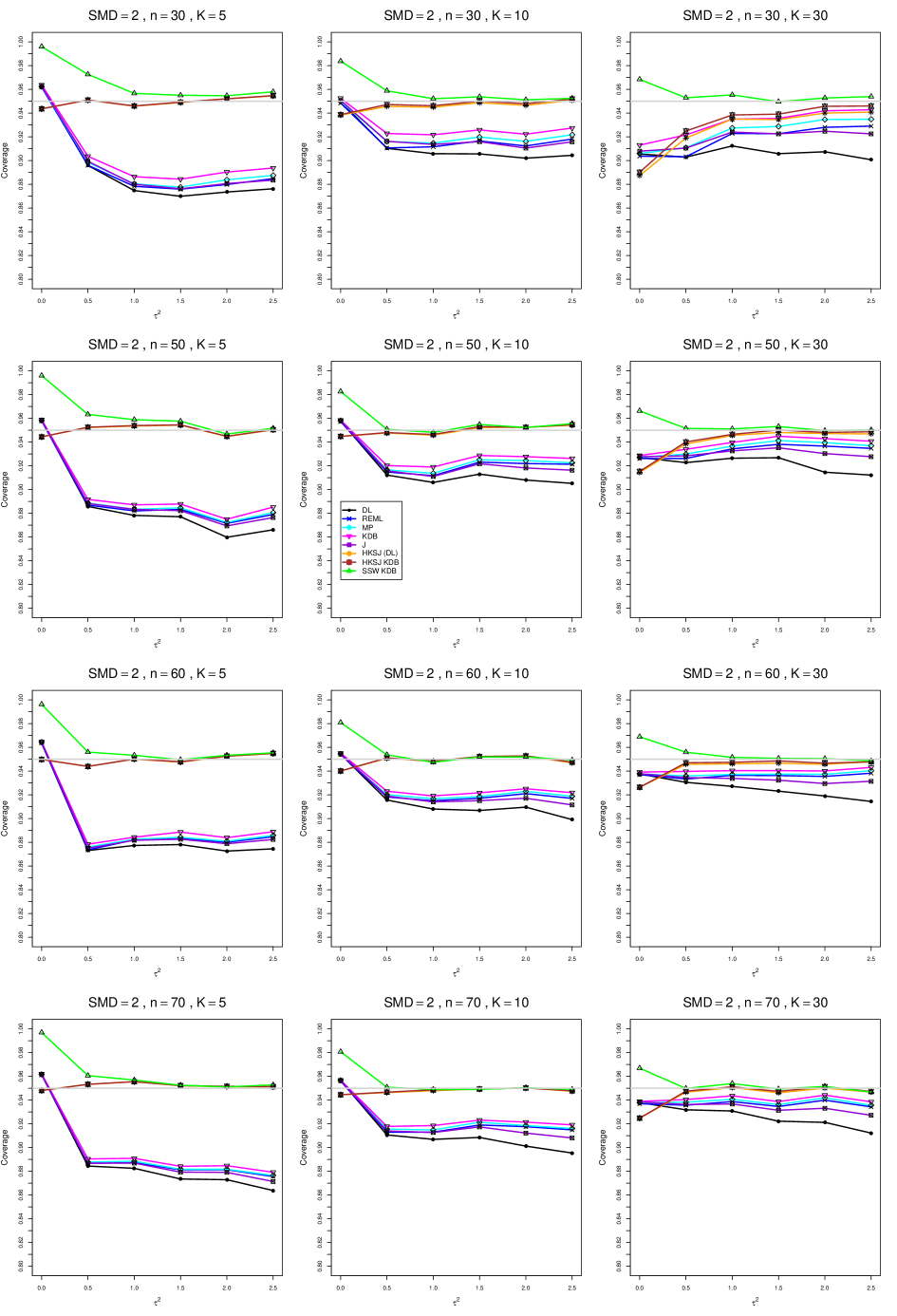
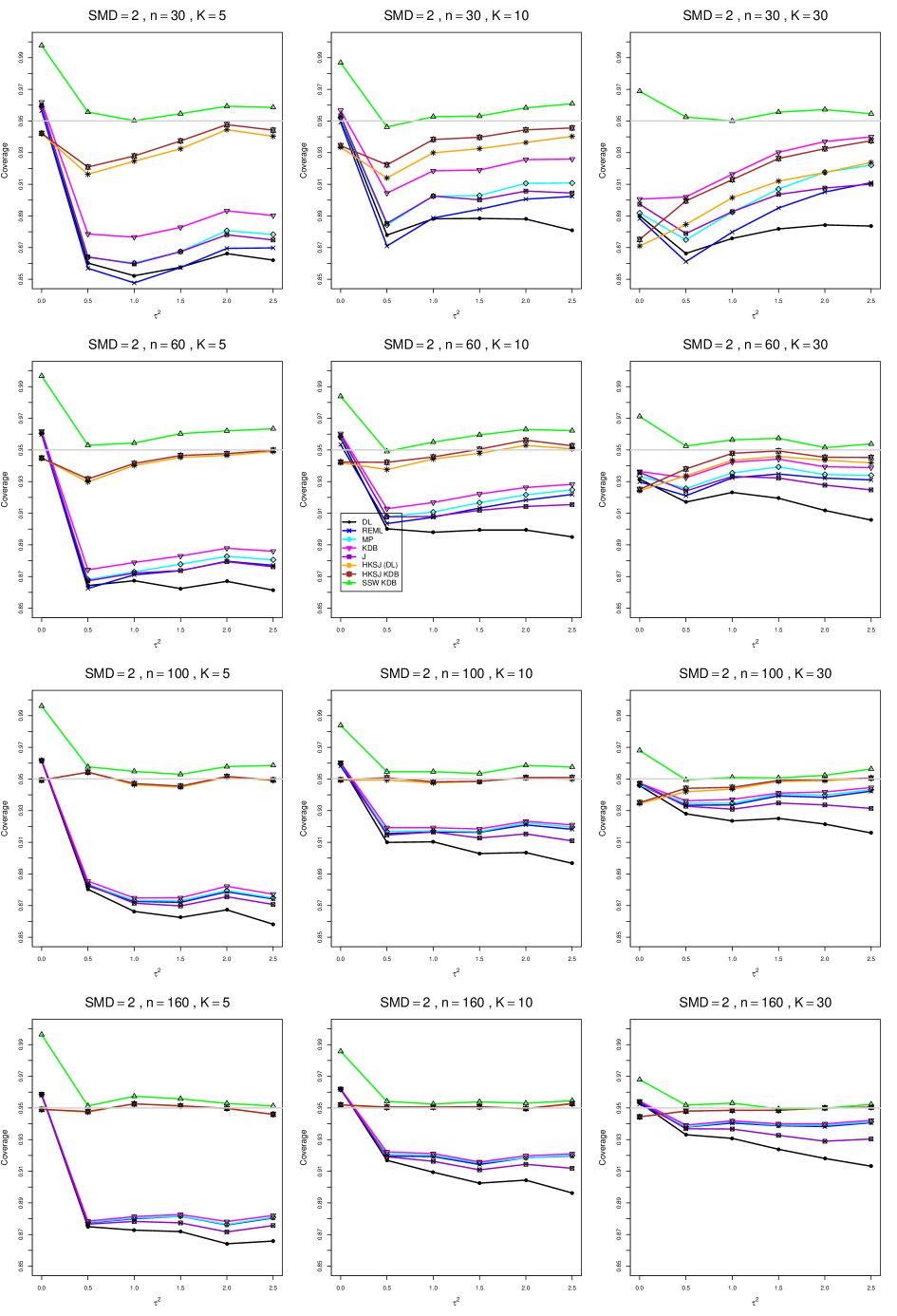
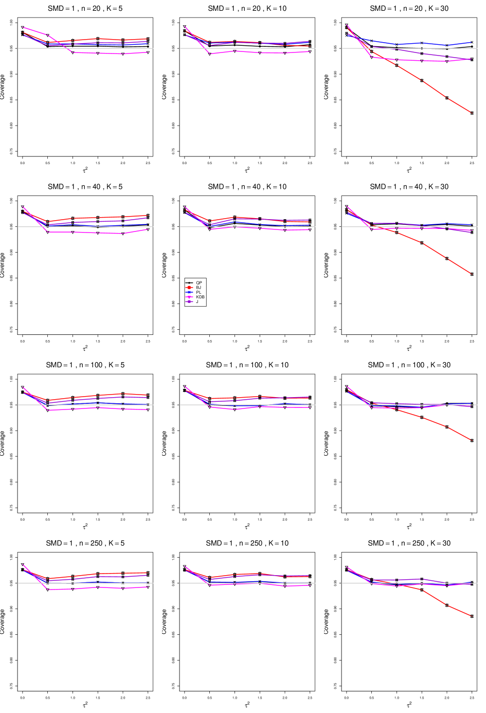
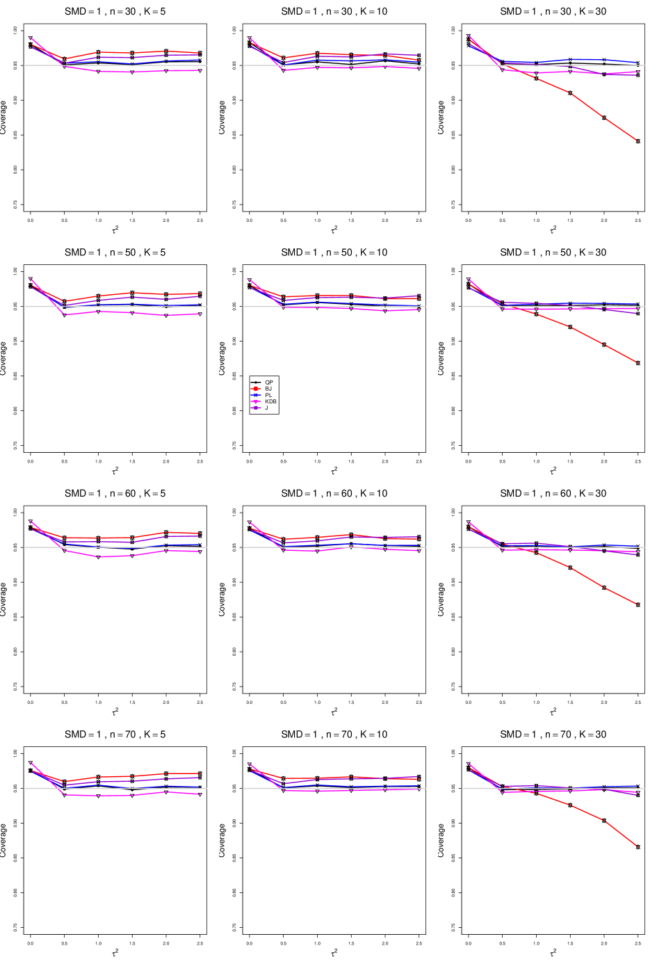
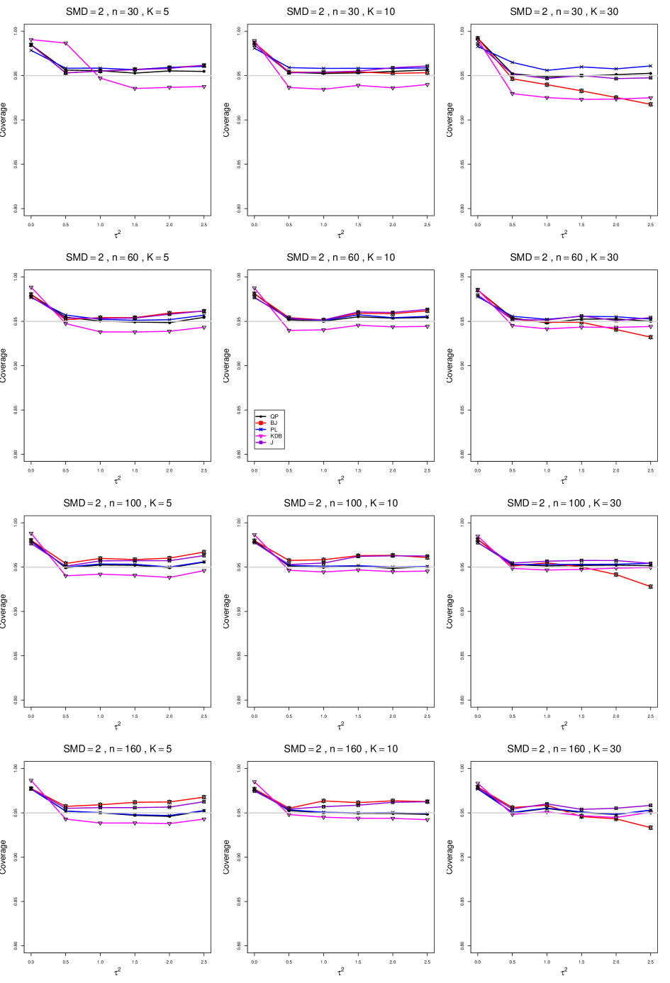
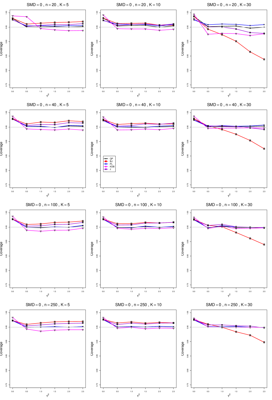
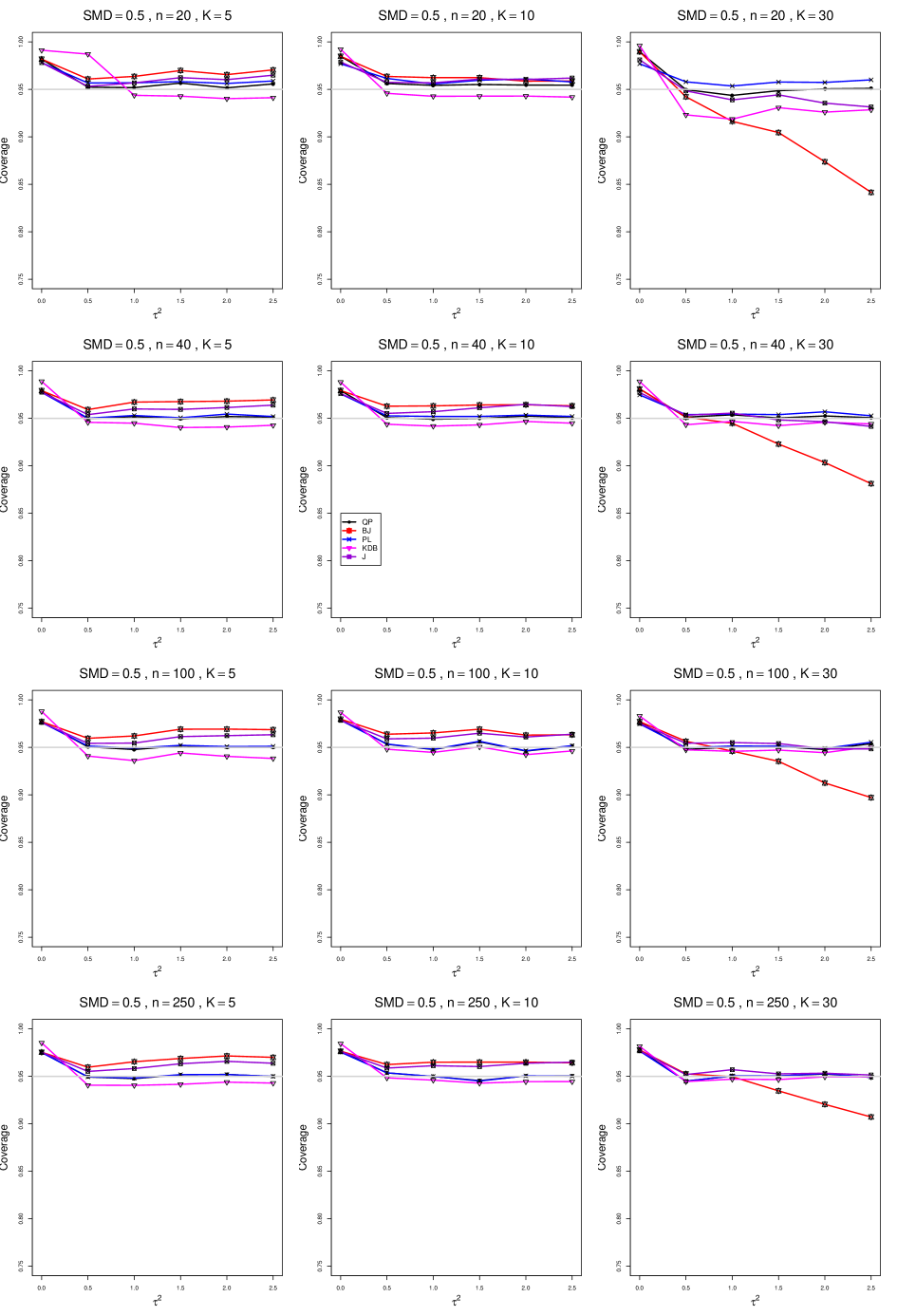
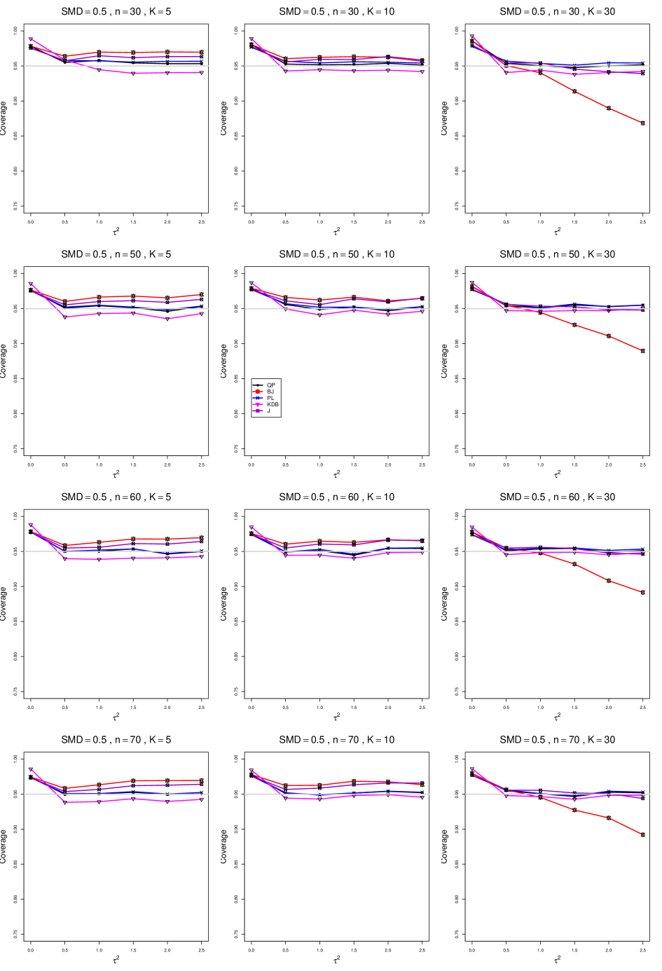
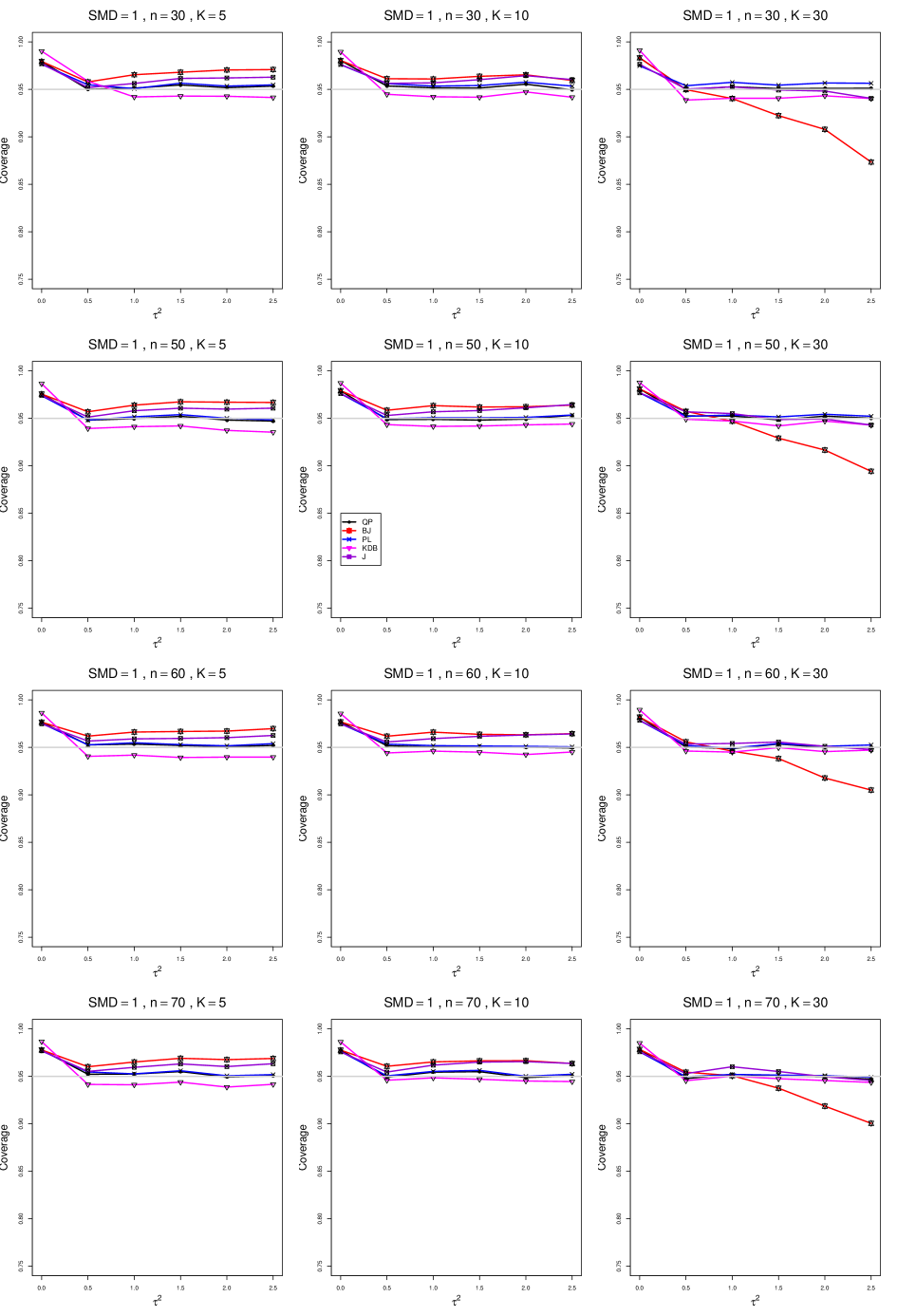
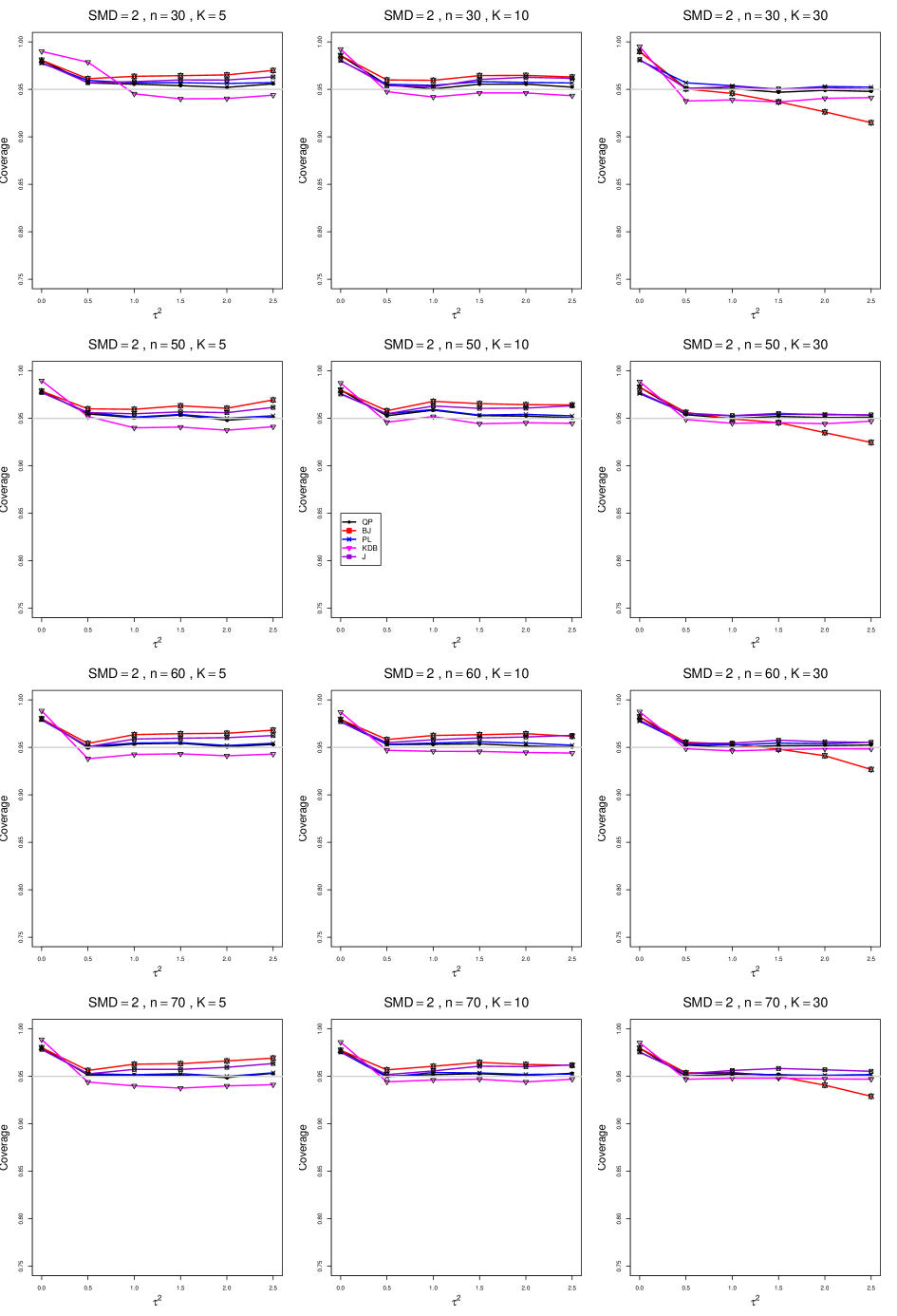
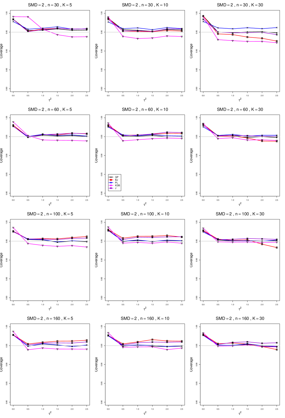
8.4 Coverage in estimation of (Appendix B2)
Coverage of the estimators that rely on inverse-variance weights and normal critical values (DL, REML, MP, KDB, and J) is influenced most by ( versus ) and . At their coverage is around .97, but at (when and ) it is mostly below .95: .90 to .91 when , .92 to.94 when , and .93 to .95+ when . As increases, their coverage either is flat (REML, MP, and KDB) or decreases (DL, J). DL almost always has the lowest coverage, and the gap between it and J widens as increases.
Except for the effect of on SSW KDB at (above .99 when , decreasing to .97 when ) and below-nominal coverage of HKSJ and HKSJ KDB in a region whose definition involves mainly , (or ), , and , the coverage of SSW and the HKSJ-type estimators is close to .95 for all and . The challenging situations in that region generally involve or , the smaller or , or , and the smaller . For example, when and or and , coverage can be as low as .84 when .
When , coverage of DL, REML, MP, KDB, and J increases as increases, usually staying below .95.
The effect of on coverage is slight except for some situations involving . When and , all of the estimators except SSW KDB have low coverage at , ranging from to .86. Their traces rise as increases; when , KDB and HKSJ KDB are almost .94, and DL is .86 (up from .84). The pattern is similar when and , but much reduced.
When , coverage decreases slightly as or increases (except for SSW and the two HKSJ-type estimators); coverage is somewhat lower when sample sizes are unequal.
The plots show at most slight differences between and .
In summary, except when and , HKSJ and HKSJ KDB have coverage closest to .95; they differ little, and departures from .95 (toward lower coverage) are seldom serious. SSW KDB is rather conservative when and for other when . Otherwise it provides reliable, albeit slightly conservative, coverage. When and , SSW KDB is the best alternative. All of the estimators that use inverse-variance weights and critical values from the normal distribution (DL,REML, J, MP, and KDB) often have coverage substantially below .95.
9 Discussion: Practical implications for meta-analysis
The results of our simulations for SMD give a rather disappointing picture. In brief:
Because the study-level effects and their variances are related (cf. Equation (2.1) for SMD), the performance of all statistical methods depends on the effect measures, estimates of overall effects are biased, and coverage of confidence intervals is too low, especially for small sample sizes.
The conventional wisdom is that these deficiencies do not matter, as meta-analysis usually deals with studies that are “large,” so all these little problems are automatically resolved. Unfortunately, this is not true, even in medical meta-analyses; in Issue 4 of the Cochrane Database 2004, the maximum study size was or less in of meta-analyses with that used SMD as an effect measure, and less than in of them (our own analysis). We have not surveyed typical study sizes in psychology, but Sánchez-Meca and Mar´ın-Mart´ınez (2010), promoting MA in psychological research, use an example with 24 studies in which the smallest study size is and the largest is . In ecology, typical sample sizes are between 4 and 25 (Hamman et al., 2018). An effect-measure-specific estimator of , such as KDB for SMD, can reduce inherent biases.
Arguably, the main purpose of a meta-analysis is to provide point and interval estimates of an overall effect.
Usually, after estimating the between-study variance , inverse-variance weights are used in estimating the overall effect (and, often, its variance). This approach relies on the theoretical result that, for known variances, and given unbiased estimates , it yields a Uniformly Minimum-Variance Unbiased Estimate (UMVUE) of . In practice, however, the true within-study variances are unknown, and use of the estimated variances makes the inverse-variance-weighted estimate of the overall effect biased.
Consumers routinely expect point estimates to have no (or small) bias and CIs to have (close to) nominal coverage. Thus, the IV-weighted approach is unsatisfactory because, in general, it cannot produce an unbiased estimate of an overall effect.
A pragmatic approach to unbiased estimation of uses weights that do not involve estimated variances of study-level estimates, for example, weights proportional to the study sizes . Hunter and Schmidt (1990) and Shuster (2010), among others, have proposed such weights, and Mar´ın-Mart´ınez and Sánchez-Meca (2010) and Hamman et al. (2018) have studied the method’s performance by simulation for SMD. We prefer to use weights proportional to an effective sample size, ; these are the optimal inverse-variance weights for SMD when and . Thus, the overall effect is estimated by , and its variance is estimated by Equation (5.1). Hamman et al. (2018) use weights proposed by Hedges (1982), which differ slightly for very small sample sizes.
A good estimator of , such as MP or KDB, can be used as . Further, confidence intervals for centered at with in Equation (5.1) can be used.
This approach based on SSW requires further study. For example, in the confidence intervals we have used critical values from the -distribution on degrees of freedom, but we have not yet examined the actual sampling distribution of SSW. The raw material for such an examination is readily available: For each situation in our simulations, each of the replications yields an observation on the sampling distribution of SSW.
Funding
The work by E. Kulinskaya was supported by the Economic and Social Research Council [grant number ES/L011859/1].
Appendices
-
•
Appendix A. SMD: Plots for bias and coverage of .
-
•
Appendix B. SMD: Plots for bias and coverage of standardized mean difference .
References
- Biggerstaff and Jackson [2008] Brad J Biggerstaff and Dan Jackson. The exact distribution of Cochran’s heterogeneity statistic in one-way random effects meta-analysis. Statistics in Medicine, 27(29):6093–6110, 2008.
- Cohen [1988] J Cohen. Statistical Power Analysis for the Behavioral Sciences. New York: Academic Press, 1988.
- DerSimonian and Laird [1986] Rebecca DerSimonian and Nan Laird. Meta-analysis in clinical trials. Controlled Cinical Trials, 7(3):177–188, 1986.
- Ferguson [2009] Christopher J Ferguson. An effect size primer: A guide for clinicians and researchers. Professional Psychology: Research & Practice, 40(5):532–538, 2009.
- Friedrich et al. [2008] Jan O Friedrich, Neill KJ Adhikari, and Joseph Beyene. The ratio of means method as an alternative to mean differences for analyzing continuous outcome variables in meta-analysis: a simulation study. BMC Medical Research Methodology, 8:32, 2008.
- Hamman et al. [2018] Elizabeth A. Hamman, Paula Pappalardo, James R. Bence, Scott D. Peacor, and Craig W. Osenberg. Bias in meta-analyses using Hedges’ d. Ecosphere, 9(9):e02419, 2018. doi: 10.1002/ecs2.2419. URL https://esajournals.onlinelibrary.wiley.com/doi/abs/10.1002/ecs2.2419.
- Hartung and Knapp [2001] Joachim Hartung and Guido Knapp. A refined method for the meta-analysis of controlled clinical trials with binary outcome. Statistics in Medicine, 20(24):3875–3889, 2001.
- Hedges [1982] Larry V Hedges. Estimation of effect size from a series of independent experiments. Psychological Bulletin, 92(2):490–499, 1982.
- Hedges [1983] Larry V Hedges. A random effects model for effect sizes. Psychological Bulletin, 93(2):388–395, 1983.
- Hedges and Olkin [1985] Larry V Hedges and Ingram Olkin. Statistical Methods for Meta-Analysis. San Diego, California: Academic Press, 1985.
- Higgins et al. [2009] Julian P T Higgins, Simon G Thompson, and David J Spiegelhalter. A re-evaluation of random-effects meta-analysis. Journal of the Royal Statistical Society, Series A, 172(1):137–159, 2009.
- Higgins and Green [2011] Julian P.T. Higgins and Sally Green, editors. Cochrane Handbook for Systematic Reviews of Interventions, Version 5.1.0 [updated March 2011]. The Cochrane Collaboration, 2011. URL http://handbook.cochrane.org.
- Hunter and Schmidt [1990] John E Hunter and Frank L Schmidt. Methods of Meta-analysis: Correcting Error and Bias in Research Findings. Sage Publications, Inc, 1990.
- Jackson [2013] Dan Jackson. Confidence intervals for the between-study variance in random effects meta-analysis using generalised Cochran heterogeneity statistics. Research Synthesis Methods, 4(3):220–229, 2013.
- Kulinskaya et al. [2011] Elena Kulinskaya, Michael B Dollinger, and Kirsten Bjørkestøl. Testing for homogeneity in meta-analysis I. The one-parameter case: standardized mean difference. Biometrics, 67(1):203–212, 2011.
- Kulinskaya et al. [2014] Elena Kulinskaya, Stephan Morgenthaler, and Robert G Staudte. Combining statistical evidence. International Statistical Review, 82(2):214–242, 2014.
- Langan et al. [2018] Dean Langan, Julian P. T. Higgins, Dan Jackson, Jack Bowden, Areti Angeliki Veroniki, Evangelos Kontopantelis, and Wolfgang Viechtbauer. A comparison of heterogeneity variance estimators in simulated random-effects meta-analyses. Research Synthesis Methods, to appear, 2018.
- Li et al. [1994] Yuanzhang Li, Li Shi, and H Daniel Roth. The bias of the commonly-used estimate of variance in meta-analysis. Communications in Statistics–Theory and Methods, 23(4):1063–1085, 1994.
- Lin [2018] Lifeng Lin. Bias caused by sampling error in meta-analysis with small sample sizes. PLoS ONE, 13(9):e0204056, 2018.
- Mandel and Paule [1970] John Mandel and Robert C Paule. Interlaboratory evaluation of a material with unequal numbers of replicates. Analytical Chemistry, 42(11):1194–1197, 1970.
- Mar´ın-Mart´ınez and Sánchez-Meca [2010] Fulgencio Marín-Martínez and Julio Sánchez-Meca. Weighting by inverse variance or by sample size in random-effects meta-analysis. Educational and Psychological Measurement, 70(1):56–73, 2010.
- Møller and Jennions [2002] Anders Møller and Michael D Jennions. How much variance can be explained by ecologists and evolutionary biologists? Oecologia, 132(4):492–500, 2002.
- Petropoulou and Mavridis [2017] Maria Petropoulou and Dimitris Mavridis. A comparison of 20 heterogeneity variance estimators in statistical synthesis of results from studies: a simulation study. Statistics in Medicine, 36(27):4266–4280, 2017.
- Rukhin [2009] Andrew L Rukhin. Weighted means statistics in interlaboratory studies. Metrologia, 46(3):323–331, 2009.
- Sánchez-Meca and Mar´ın-Mart´ınez [2000] Julio Sánchez-Meca and Fulgencio Marín-Martínez. Testing the significance of a common risk difference in meta-analysis. Computational Statistics & Data Analysis, 33(3):299–313, 2000.
- Sánchez-Meca and Mar´ın-Mart´ınez [2010] Julio Sánchez-Meca and Fulgencio Marín-Martínez. Meta-analysis in psychological research. International Journal of Psychological Research, 3(1):150–162, 2010.
- Shuster [2010] Jonathan J Shuster. Empirical vs natural weighting in random effects meta-analysis. Statistics in Medicine, 29(12):1259–1265, 2010.
- Sidik and Jonkman [2002] K. Sidik and J. N. Jonkman. A simple confidence interval for meta-analysis. Statistics in Medicine, 21(21):3153–3159, 2002.
- Sidik and Jonkman [2006] Kurex Sidik and Jeffrey N Jonkman. Robust variance estimation for random effects meta-analysis. Computational Statistics & Data Analysis, 50(12):3681–3701, 2006.
- Veroniki et al. [2016] Areti Angeliki Veroniki, Dan Jackson, Wolfgang Viechtbauer, Ralf Bender, Jack Bowden, Guido Knapp, Oliver Kuss, Julian P T Higgins, Dean Langan, and Georgia Salanti. Methods to estimate the between-study variance and its uncertainty in meta-analysis. Research Synthesis Methods, 7(1):55–79, 2016.
- Viechtbauer [2005] Wolfgang Viechtbauer. Bias and efficiency of meta-analytic variance estimators in the random-effects model. Journal of Educational and Behavioral Statistics, 30(3):261–293, 2005.
- Viechtbauer [2007] Wolfgang Viechtbauer. Confidence intervals for the amount of heterogeneity in meta-analysis. Statistics in Medicine, 26(1):37–52, 2007.
10 Appendices
A1. Bias of point estimators of for .
For bias of , each figure corresponds to a value of , a value of , and a set of values of (= 20, 40, 100, 250 or 30, 50, 60, 70) or .
Each figure contains a panel (with on the horizontal axis) for each combination of n (or ) and .
The point estimators of are
-
•
DL (DerSimonian-Laird)
-
•
REML (restricted maximum likelihood)
-
•
MP (Mandel-Paule)
-
•
KDB (improved moment estimator based on Kulinskaya, Dollinger and Bjørkestøl (2011))
-
•
J (Jackson)
A2. Coverage of of interval estimators of for .
For coverage of , each figure corresponds to a value of , a value of , and a set of values of (= 20, 40, 100, 250 or 30, 50, 60, 70) or .
Each figure contains a panel (with on the horizontal axis) for each combination of n (or ) and .
The interval estimators of are
-
•
QP (Q-profile confidence interval)
-
•
BJ (Biggerstaff and Jackson interval )
-
•
PL (Profile likelihood interval)
-
•
KDB ( KDB - improved Q-profile method based on Kulinskaya, Dollinger and Bjørkestøl (2011))
-
•
J (Jackson’s interval)
B1. Bias and mean squared error of point estimators of for .
For bias of , each figure corresponds to a value of , a value of , and a set of values of (= 20, 40, 100, 250 or 30, 50, 60, 70) or .
Figures for mean squared error (expressed as the ratio of the MSE of SSW to the MSEs of the inverse-variance-weighted estimators that use the MP or KDB estimator of ) use the above values of and q but only n = 20, 40, 100, 250.
Each figure contains a panel (with on the horizontal axis) for each combination of n (or ) and .
The point estimators of are
-
•
DL (DerSimonian-Laird)
-
•
REML (restricted maximum likelihood)
-
•
MP (Mandel-Paule)
-
•
KDB (improved moment estimator based on Kulinskaya, Dollinger and Bjørkestøl (2011))
-
•
J (Jackson)
-
•
SSW (sample-size weighted)
B2. Coverage of interval estimators for .
For coverage of , each figure corresponds to a value of (= 0, 0.5, 1, 1.5, 2 , 2.5), a value of q (= .5, .75), and a set of values of n (= 20, 40, 100, 250 or 30, 50, 60, 70) or (= 30, 60, 100, 160).
Each figure contains a panel (with on the horizontal axis) for each combination of n (or ) and .
The interval estimators of are the companions to the inverse-variance-weighted point estimators
-
•
DL (DerSimonian-Laird)
-
•
REML (restricted maximum likelihood)
-
•
MP (Mandel-Paule)
-
•
KDB (improved moment estimator based on Kulinskaya, Dollinger and Bjørkestøl (2011))
-
•
J (Jackson)
and
-
•
HKSJ (Hartung-Knapp-Sidik-Jonkman)
-
•
HKSJ KDB (HKSJ with KDB estimator of )
-
•
SSW (SSW as center and half-width equal to critical value from
times estimated standard deviation of SSW with = .