Simulations of Blood Flow in Plain Cylindrical and Constricted Vessels with Single Cell Resolution
Abstract
Understanding the physics of blood is challenging due to its nature as a suspension of soft particles and the fact that typical problems involve different scales. This is valid also for numerical investigations. In fact, many computational studies either neglect the existence of discrete cells or resolve relatively few cells very accurately. The authors recently developed a simple and highly efficient yet still particulate model with the aim to bridge the gap between currently applied methods. The present work focuses on its applicability to confined flows in vessels of diameters up to . For hematocrit values below , a dependence of the apparent viscosity on the vessel diameter in agreement with experimental literature data is found.
I Introduction
Human blood can be approximated as a suspension of deformable red blood cells (RBCs, also called erythrocytes) in a Newtonian liquid, the blood plasma. The other constituents like leukocytes and thrombocytes (blood platelets) can be neglected due to their low volume concentrations.1 Typical concentrations for RBCs are to under physiological conditions. In the absence of external stresses, erythrocytes assume the shape of biconcave discs of approximately diameter.2 An understanding of their effect on the rheology and the clotting behavior of blood is necessary for the study of pathological deviations in the body and the design of microfluidic devices for improved blood analysis.
Well-established methods for the computer simulation of blood flow consist of an elaborate model of deformable cell membranes coupled to the surrounding plasma described by particle-based hydrodynamic methods3; 4, the lattice Boltzmann (LB) method5; 6, or the boundary integral method7. Others restrict themselves to a continuous description at larger scales.8 Our motivation is to bridge the gap between both classes of models by an intermediate approach that was published recently.9 During the last decade, other groups already presented coarse-grained yet particulate models for blood at the mesoscale. Both Fenech et al.10 and Chesnutt and Marshall11 developed discrete element models for the aggregation of large numbers of RBCs in two and three dimensions. These works, however, do not explicitly resolve the hydrodynamics of the blood plasma. Approaches based on dissipative particle dynamics (DPD) directly model hydrodynamics. Boryczko et al.12 applied their model that comprises plasma, deformable red cells, and capillary walls to the study of fibrin aggregation in the microcirculation. Filipovic et al.13 employed DPD for the study of platelet adhesion to vessel walls and Pivkin et al.14 for the investigation of the effect of RBCs on the aggregation of blood platelets. Another simulation method that is well suited to account for hydrodynamics in confined geometries is the LB method which consequently has been applied in blood models of various levels of detail. Additionally to the models mentioned before already which are either based on a continuous fluid8 or a suspension of fully deformable cells5; 6, there exist also more coarse grained particulate models employing the LB method: Sun et al.15 model both red and white blood cells in two dimensions as rigid ellipses and spheres, the latter of which are, however, equipped with an elaborate wall-adhesion model. In the work by Hyakutake et al.16 the behavior of two-dimensional rigid spheres representing RBCs at microvascular bifurcations is studied.
Our coarse-grained blood model aims at a minimal resolution of red blood cells which allows for a simple and highly efficient but still particulate description of blood as a suspension. Still, we do not give up explicitly modeling the suspending blood plasma or accounting for the non-spherical shape of RBCs. The ultimate goal is to perform large-scale simulations that allow to study the flow in realistic geometries but also to link bulk properties, for example the effective viscosity, to phenomena at the level of single erythrocytes. Only a computationally efficient description allows the reliable accumulation of statistical properties in time-dependent flows which is necessary for this task. The improved understanding of the dynamic behavior of blood might be used for the optimization of macroscopic simulation methods.
The main idea of our model is to distinguish between the long-range hydrodynamic coupling of cells and the short-range interactions that are related to the complex mechanics, electrostatics, and the chemistry of the membranes. The short-range behavior of RBCs is described on a phenomenological level by means of anisotropic model potentials.9 Long-range hydrodynamic interactions are accounted for by means of an LB method.17 Our model is well suited for the implementation of complex boundary conditions and an efficient parallelization on parallel supercomputers. Both are necessary for the study of realistic systems like branching vessels and the accumulation of statistically relevant data in bulk flow situations. In Section II and III, we briefly explain our approach. For an extended description we refer to our earlier publication.9 Section IV contains—next to parameter studies and a review of earlier results9—an investigation of the apparent blood viscosity in tubes and the related Fåhræus-Lindqvist effect. It closes with a qualitative view on constrictions and branching points in capillaries and data regarding the scalability of the code. In Section V, the conclusions from our work are drawn.
II Hydrodynamic part of the model
We apply a Bhatnagar-Gross-Krook (BGK) LB method for modeling the blood plasma.18 See for example the book of Succi for a comprehensive introduction.17 The single particle distribution function resembles the fluid traveling with one of discrete velocities at the three-dimensional lattice position and discrete time . Its evolution in time is determined by the lattice Boltzmann equation
| (1) |
with
| (2) |
being the BGK-collision term with a single relaxation time . The equilibrium distribution function is an expansion of the Maxwell–Boltzmann distribution. and can be identified as density and momentum. In the limit of small velocities and lattice spacings the Navier–Stokes equations are recovered with a kinematic viscosity of , where in this study.
For a coarse-grained description of the hydrodynamic interaction of cells and blood plasma, a method similar to the one by Aidun et al. modeling rigid particles of finite size is applied.19; 20 Starting point is the mid-link bounce-back boundary condition: the confining geometry is discretized on the lattice and all internal nodes are turned into fluid-less wall nodes. If is such a node the updated distribution at is determined as
| (3) |
with
| (4) |
This corresponds to replacing the local distribution in direction with the post-collision distribution of the opposite direction . To model boundaries moving with velocity , Equation (3) needs to be modified. The resulting update rule
| (5) |
with
| (6) |
was chosen consistently with for the general case . The lattice weights and the speed of sound are constants for a given set of discrete velocities. The momentum
| (7) |
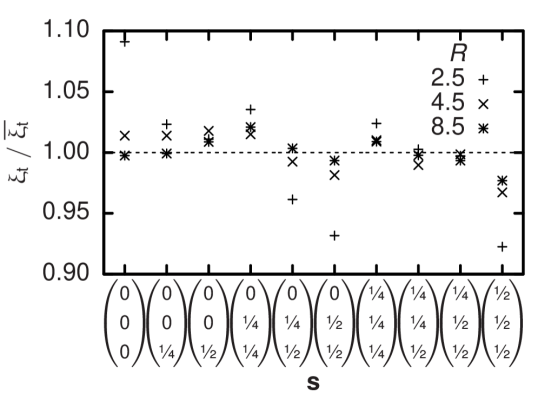
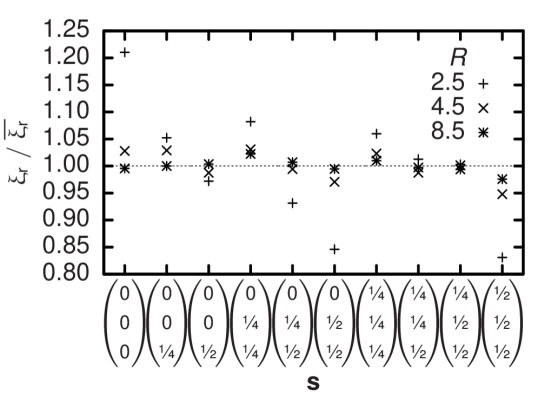
which is transferred during each time step by each single bounce-back process is used to calculate the resulting force on the boundary. A freely moving particle is modeled by such moving walls and is defined by its continuous position : all lattice nodes within a given theoretical particle volume—e. g. a sphere—centered at are considered a wall and Equation (5) is applied to links connected to its surface. When changes, eventually the particle’s discretization on the lattice needs to be updated. During this process, fluid nodes are created or vanish and the related change in total fluid momentum is balanced by an additional force on the respective particle. Still, the discretized particle shape undergoes fluctuations depending on the offset of to the nearest lattice node. Their effect on hydrodynamics is quantified by measuring the translational and rotational drag coefficient and of a sphere of radius at a selection of different offset vectors . Since the model can be calibrated by assuming an effective hydrodynamic radius different from 21, the drag coefficients are not normalized to the theoretical values but to their respective averages. The results in Figures 1 and 2 show that discretization effects depend on but even for typical deviations are not larger than . Typically, deviations in the rotational drag coefficient appear to be two times larger than the corresponding translational values.
In contrast to the biconcave equilibrium shape of physiological RBCs and the previous tests with spherical particles we choose a simplified ellipsoidal geometry that is defined by two distinct half-axes and parallel and perpendicular to the unit vector which points along the direction of the axis of rotational symmetry of each particle . Since the cell-fluid interaction volumes are rigid we need to allow them to overlap in order to account for the deformability of real erythrocytes. We assume a pair of mutual forces
| (8) |
and
| (9) |
at each cell-cell link. This is exactly the momentum transfer during one time step due to the rigid-particle algorithm for a resting particle and an adjacent site with resting fluid at equilibrium and initial density and thus compensates for the static fluid pressure. In case of close contact of cells with the confining geometry we proceed in a similar manner as for two cells but ignore forces on the system walls.
III Model potentials
In order to account for the complex behavior of real RBCs at small distances we add phenomenological pair potentials between cells. The idea is to develop simple model potentials and adjust their free parameters in order to match the pair interactions of cells. In a very similar way, the well-known Lennard-Jones potential is applied in classical molecular dynamics simulations to model atomic interactions. A fit can be achieved by comparison of simulation results and experimental data from the literature, specially regarding blood rheology. For the moment, we concentrate on high shear rates where aggregative effects play no role.22 Therefore the model potential has to account only for deformation effects. As a simple way to describe elastic deformability, we use the repulsive branch of a Hookean spring potential
| (10) |
for the scalar displacement of two cells and . With respect to the disc-shape of RBCs, we follow the approach of Berne and Pechukas23 and choose the energy and range parameters
| (11) |
and
| (12) |
as functions of the orientations and of the cells and their normalized center displacement . We achieve an anisotropic potential with a zero-energy surface that is approximately that of ellipsoidal discs. Their half-axes parallel and perpendicular to the symmetry axis enter Equation (11) and (12) via and whereas determines the potential strength. For modeling the cell-wall interaction we assume a sphere with radius at every lattice node on the surface of a vessel wall and implement similar forces as for the cell-cell interaction. Using
| (13) |
as a range parameter with and allows to scale a potential with radial symmetry to fit for the description of the interaction of a sphere and an ellipsoidal disc.23 The parameter remains constant in this case. is the normalized center displacement of cell and a wall node .
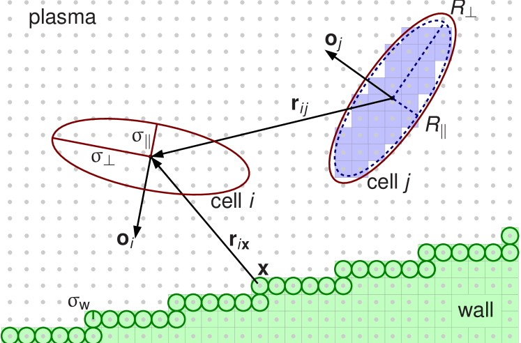
Figure 3 shows a two-dimensional cut as an outline of the full model. For two RBCs the inner volume implementing the cell-plasma interaction with half axes and is shown. Also depicted are the larger volumes that are defined by the range parameters and of the cell-cell and cell-wall interaction. A section of a vessel wall is visualized. The cell-wall interaction is based on the assumption of spheres with radius at the location of the surface wall nodes. The forces and torques emerging from the interaction of the cells with the fluid, other RBCs, and walls are integrated by a leap-frog scheme in order to evolve the system in time. Both the LB routines and the ones employed for treatment of the suspended cells use the same domain decomposition. For more detailed information concerning the model we refer to.9
IV Results
All quantities can be converted from simulation units to physical units by multiplication with products of integer powers of the conversion factors , , and for space, time, and mass. As a convention in this work, primed variables are used to distinguish quantities given in physical units from the same unprimed variable measured in lattice units. Based on experimental measurements of RBC geometries,2 the half-axes of the simplified volume defining the cell-cell interaction in our model are set to
| (14) |
When choosing the spatial resolution quantified by the physical distance corresponding to one lattice spacing, a compromise needs to be found: A low resolution severely reduces the computational effort but also reduces numerical accuracy. We decide for 9 which allows a contiguous and closed volume of the cell-fluid interaction which still is completely comprised within the cell-cell interaction volume Equation (14). On the actual values of and we decide after studying their influence on the apparent viscosity of the model suspension in plane Couette flow.
Supposing that matches the kinematic plasma viscosity of , the time discretization is determined as . Since the largest shear rates employed in this work are of the order of , sufficient temporal resolution is provided. is chosen arbitrarily. All shear flow simulations reported here are performed on a system with a size of lattice units in - and lattice units in - and -direction or of real blood. Between the two -side planes a constant offset of the local fluid velocities in -direction is imposed by an adaption of the Lees-Edwards shear boundary condition to the LB method.24 The apparent viscosity is calculated from the average shear rate and shear stress.9 Recently, an alternative method of viscosity measurement based on Kolmogorov flow was demonstrated which allows the employment of more simple periodic boundary conditions.25
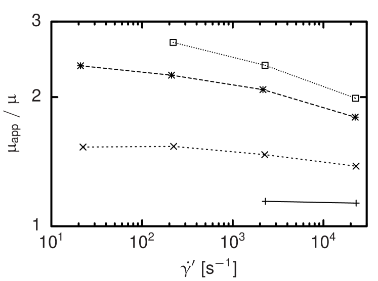
The influence of the volume of the cell-fluid interaction is studied as a function of the shear rate. Figure 4 shows the result for different and at a cell number concentration that varies by less than . Generally, shear thinning is visible, but both the absolute viscosities and the change in viscosity per shear rate increase significantly for larger interaction volumes. Based on this and further parameter studies,9 we choose with the largest value investigated here and assuming obtain or and measured in lattice units. A sphere with equal volume has a radius of . Figures 1 and 2 suggest that at this resolution, we have to expect discretization errors of the order of some percents that are acceptable for our approach.
In further simulations the effect of the stiffness parameter of the cell-cell potential is studied. The viscosity as a function of the shear rate increases with increasing . For very stiff cells this dependence on the shear rate decreases considerably which is in asymptotic consistency with the experimental results of Chien22 who measured the apparent shear viscosity of a suspension of artificially hardened RBCs and found a significantly increased yet mostly constant viscosity. At a cell-fluid volume concentration of which seems sufficiently close to the hematocrit of in the measurements done by Chien22 to justify a quantitative comparison, we find best agreement for and use this parametrization for all following investigations.9
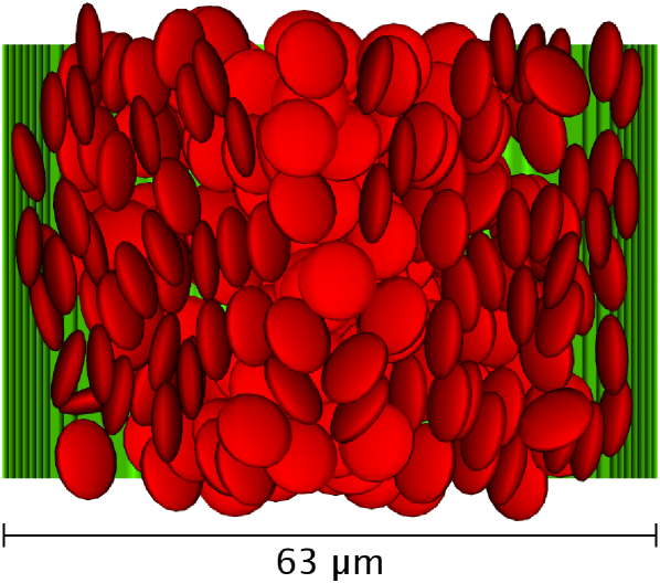
We now confine our model suspension in a cylindrical channel of diameter and a length of with periodic boundaries. Both cells and plasma are steadily driven by a volume force equivalent to a pressure gradient . We arbitrarily choose for the strength of the cell-wall interaction as a value that reliably prevents cells from penetrating the vessel wall. Figure 5 visualizes the cells as the volumes defined by the cell-cell interaction and the channel wall as midplane between fluid and wall nodes in the case of and . The pseudo-shear rate, which is defined via the volume flow rate , is . A preferential alignment of the cells largely perpendicular to the velocity gradient is visible.
We compare radial velocity profiles for different flow velocities, a cell-fluid volume concentration of , and . While for high velocities the result looks parabolic in the central region, there is increasing blunting of the profile when the flow rate is reduced. The blunting can be understood as a consequence of the shear-thinning behavior of the model and is qualitatively consistent with experimental data from the literature.1 Generally, apparent slip is visible close to the vessel wall. It is due to a cell depletion layer that to some extent can be controlled via . Thus, the observations can partly be described by an existing model assuming a homogeneous core region with high hematocrit and consequently high viscosity and a cell-depleted boundary layer close to the vessel wall.9; 26
As it is well known, the formation of this cell depletion layer influences the flow resistance of vessels which can be expressed in terms of their apparent viscosity.26 By inserting the measured volume flow rate through a cylindrical vessel into the theoretical expression for a Newtonian fluid
| (15) |
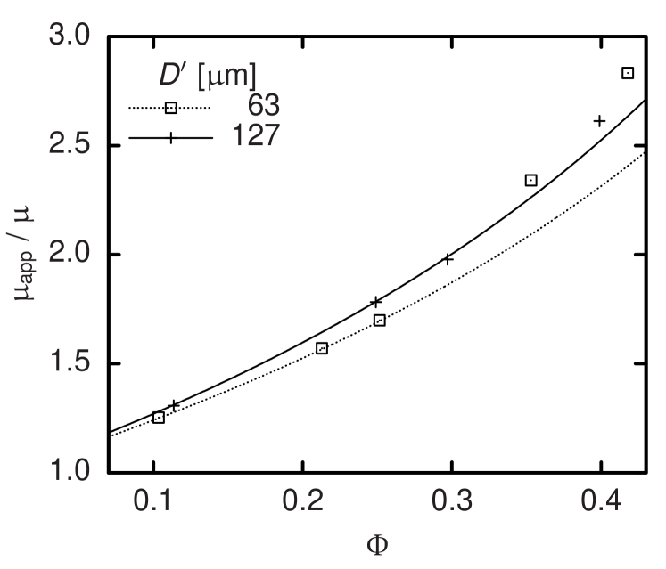
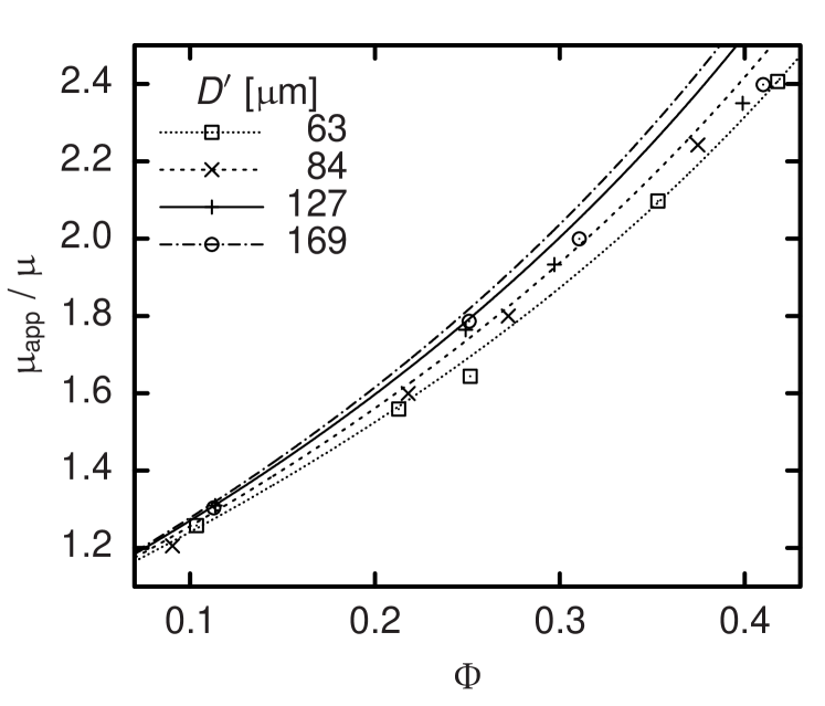
and solving for , the respective apparent viscosity can be determined. Except for , all known quantities in Equation (15) are constant and set as parameters of our simulation code. Only the flow rate undergoes stochastic fluctuations and—at the beginning of each simulation—shows a strong time dependence as the system relaxes from an arbitrary initial condition to a macroscopically steady state. Thus, typical simulations last for up to time steps corresponding to of physical time. is averaged over typically and its statistical error serves to estimate the accuracy of the resulting viscosity. The main dependency of is on the hematocrit . A comparison with experimental data in the case of Couette flow was published earlier.9 However, depends also on the vessel diameter . This is known as Fåhræus-Lindqvist effect.26 Pries et al. combine a large set of experimental studies for and provide an empirical fit.27 The resulting expression for is plotted as a function of for four discrete values of as lines in Figure 6 and 7. The symbols stand for simulation results at the same diameters and pseudo-shear rates of (Figure 6) and (Figure 7). In consistency with the still significant shear-thinning that experiments22 but also our simulations9 exhibit above , our results show a clear dependency on the pseudo-shear rate, which cannot be covered by the curves by Pries et al. that were obtained from averaging over different .27 Nevertheless, a comparison confirms the agreement concerning the order of magnitude of our results and the observation that the apparent viscosity increases with . This can be explained by the decreasing relative influence of the cell depletion layer. While the effect seems captured realistically for low volume concentrations , the dependence of on becomes less clear for higher . We explain this discrepancy by the fact that the thickness of the cell-depleted layer at high is determined by a balance of the short-range interactions of cells in the core acting towards a decrease of the depletion layer thickness and the short-range interactions of cells and the vessel wall acting towards its increase. Since the method presented above models short-range interactions by means of potential forces and a constant pressure force Equation (8) and (9), velocity-dependent lubrication and lift forces can be covered only insufficiently in the case of very high volume concentrations. However, due to the Fåhræus effect,26 in smaller blood vessels is lower than the discharge hematocrit of typically –. Also the -dependence found according to Pries et al.27 and displayed in Figure 6 and 7 is not very strong for the diameters studied. Thus the actual impact of the limitation of our model concerning should not be overestimated when simulating vessels of comparable diameters.
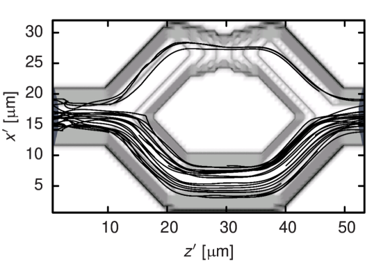
With a concluding study of the flow of nine RBCs through branching capillaries we demonstrate on a qualitative level that our coarse-grained model is able to describe problems where even single cells significantly affect the whole flow. While the diameter of the capillaries amounts to , one of the branches features a stenosis of only . A cut of this setup is visualized in Figure 8. Both tube diameters and Reynolds numbers match physiological situations.28 We vary the cell-wall interaction stiffness and find that for , the erythrocytes easily pass the constriction as expected for healthy cells.1 The trajectories of the cell centers in this case are also shown in Figure 8. They visualize that—as expected from the literature28—a clear majority of cells is drawn into the unconstricted branch due to its higher flow rate. In consequence, the branch with the stenosis features a reduced hematocrit. Figure 9, which displays the time evolution of the relative volume flow rate in the constricted branch, makes clear that for this quantity changes only due to fluctuations induced by the mutable configuration of RBCs in the system. The constricted branch gets clogged for which is also reflected by Figure 9. In the case of an intermediate value of , cells are initially stopped but due to pressure fluctuations get squeezed through the stenosis eventually. The acceleration by the cell-wall potential when leaving the constriction leads to the peaks of the flow rate visible in Figure 9.
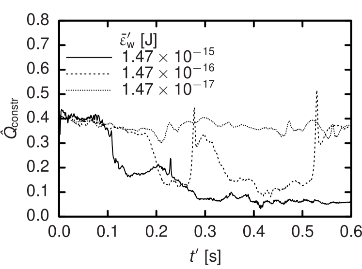
While the results for the straight channel studied first could still mostly be reproduced by a homogenous fluid with a specially tuned shear-rate or position dependent viscosity,8; 29 this is not possible at the scale of capillaries. Here, our model allows to account for clearly particulate effects like clogging or local changes of flow rate and pressure. In Figure 9, it is demonstrated that such effects can lead to a distinct unsteadiness of the local cell volume concentration which is present also in human microvascular networks.26
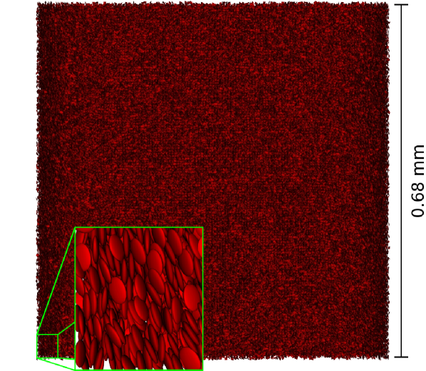
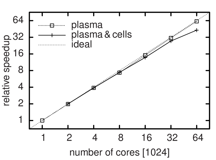
Despite the simplifications of the model, parallel supercomputers are necessary to simulate more realistic vessel networks or large bulk systems. This makes the scalability of the code crucial. For a quasi-homogenous chunk of suspension consisting of lattice sites and cells (see Figure 10) simulated on a BlueGene/P system, we achieve a parallel efficiency normalized to the case of -fold parallelism of on and still on cores. In comparison, the pure LB code without suspended RBCs shows a relative parallel efficiency of on cores. The parallel performance of the combined code is mainly limited by the relation of the interaction range of a cell to the size of the computational domain dedicated to each task. The full strong scaling behavior for up to cores is shown in Figure 11. Compared to deformable particle models,5 our method not only has a lower overall number of computations at a given resolution but is also easier to parallelize efficiently because each RBC has only six degrees of freedom.
V Conclusion
We recently developed a computational model for the coarse-grained simulation of blood flow.9 In the present work, additional bulk flow studies regarding the model parameters are shown. We further extend previous measurements of the apparent viscosity in cylindrical channels to a comparison of different tube diameters between and . While at higher hematocrit values the consistency remains limited to capturing the general behavior of the viscosity and its order of magnitude, the Fåhræus-Lindqvist effect is reproduced very similarly to experimental data for .27 With a qualitative study of unsteady flow and clogging in branching capillaries with a constriction, possible applications of our model are shown to range from bulk flow to capillary networks. Taking into account the good scalability of the code on massively parallel supercomputers, we believe that our method can help to achieve a better understanding of the links between the behavior of single cells and the properties of the encompassing larger flow structures.
Acknowledgements.
The authors acknowledge financial support from the Netherlands Organization for Scientific Research (VIDI grant of J. Harting), the TU/e High Potential Research Program, and the HPC-Europa2 project as well as computing resources from JSC Jülich (granted by PRACE), SSC Karlsruhe, CSC Espoo, EPCC Edinburgh, and SARA Amsterdam, the latter three being granted by DEISA as part of the DECI-5 project.References
- [1] H. L. Goldsmith and R. Skalak, Annu. Rev. Fluid Mech. 7, 213 (1975)
- [2] E. Evans and Y. C. Fung, Microvascular Research 4, 335 (1972)
- [3] H. Noguchi and G. Gompper, PNAS 102, 14159 (2005)
- [4] D. A. Fedosov, B. Caswell, and G. E. Karniadakis, Biophysical Journal 98, 2215 (2010)
- [5] M. M. Dupin, I. Halliday, C. M. Care, L. Alboul, and L. L. Munn, Phys. Rev. E 75, 066707 (2007)
- [6] J. Wu and C. K. Aidun, International Journal for Numerical Methods in Fluids 62, 765 (2010)
- [7] J. B. Freund, Phys. Fluids 19, 023301 (2007)
- [8] J. Boyd, J. M. Buick, and S. Green, Phys. Fluids 19, 093103 (2007)
- [9] F. Janoschek, F. Toschi, and J. Harting, Physical Review E 82, 056710 (2010)
- [10] M. Fenech, D. Garcia, H. J. Meiselman, and G. Cloutier, Annals of Biomedical Engineering 37, 2299 (2009)
- [11] J. K. W. Chesnutt and J. S. Marshall, Computers & Fluids 38, 1782 (2009)
- [12] K. Boryczko, W. Dzwinel, and D. A. Yuen, Computer Methods and Programs in Biomedicine 75, 181 (2004)
- [13] N. Filipovic, M. Kojic, and A. Tsuda, Phil. Trans. R. Soc. Lond. A 366, 3265 (2008)
- [14] I. Pivkin, P. Richardson, and G. Karniadakis, IEEE Engineering in Medicine and Biology Magazine 28, 32 (2009)
- [15] C. Sun, C. Migliorini, and L. L. Munn, Biophysical Journal 85, 208 (2003)
- [16] T. Hyakutake, T. Matsumoto, and S. Yanase, Mathematics and Computers in Simulation 72, 134 (2006)
- [17] S. Succi, The Lattice Boltzmann Equation for Fluid Dynamics and Beyond, Numerical Mathematics and Scientific Computation (Oxford University Press, 2001)
- [18] Y. H. Qian, D. d’Humières, and P. Lallemand, Europhys. Lett. 17, 479 (1992)
- [19] C. K. Aidun, Y. Lu, and E.-J. Ding, J. Fluid Mech. 373, 287 (1998)
- [20] N.-Q. Nguyen and A. J. C. Ladd, Phys. Rev. E 66, 046708 (2002)
- [21] A. J. C. Ladd, J. Fluid Mech. 271, 311 (1994)
- [22] S. Chien, Science 168, 977 (1970)
- [23] B. J. Berne and P. Pechukas, J. Chem. Phys. 56, 4213 (1972)
- [24] A. J. Wagner and J. M. Yeomans, Phys. Rev. E 59, 4366 (1999)
- [25] F. Janoschek, F. Mancini, J. Harting, and F. Toschi, Phil. Trans. R. Soc. London Series A 369, 2337 (2011)
- [26] A. S. Popel and P. C. Johnson, Annual Review of Fluid Mechanics 37, 43 (2005)
- [27] A. R. Pries, D. Neuhaus, and P. Gaehtgens, Am. J. Physiol. – Heart and Circ. Physiol. 263, H1770 (1992)
- [28] Y. C. Fung, Biomechanics. Mechanical Properties of Living Tissues (Springer, New York, 1981)
- [29] T. W. Secomb, in Modeling and Simulation of Capsules and Biological Cells, edited by C. Pozrikidis (Chapman & Hall/CRC, 2003) pp. 163–196
VI Material for table of contents
VI.1 Picture
![[Uncaptioned image]](https://cdn.awesomepapers.org/papers/83534f65-0c01-4b65-8470-fb14784cc8b2/x12.png)
VI.2 Text
The simulation of hemodynamics is a very challenging task. Recently, a scalable and simple particulate model was developed that has the potential to bridge the gap that existing methods left open. Here, the model is applied to flows in vessels of diameters up to .