Simultaneous SNP identification in association studies with missing data
Abstract
Association testing aims to discover the underlying relationship between genotypes (usually Single Nucleotide Polymorphisms, orSNPs) and phenotypes (attributes, or traits). The typically large data sets used in association testing often contain missing values. Standard statistical methods either impute the missing values using relatively simple assumptions, or delete them, or both, which can generate biased results. Here we describe the Bayesian hierarchical model BAMD (Bayesian Association with Missing Data). BAMD is a Gibbs sampler, in which missing values are multiply imputed based upon all of the available information in the data set. We estimate the parameters and prove that updating one SNP at each iteration preserves the ergodic property of the Markov chain, and at the same time improves computational speed. We also implement a model selection option in BAMD, which enables potential detection of SNP interactions. Simulations show that unbiased estimates of SNP effects are recovered with missing genotype data. Also, we validate associations between SNPs and a carbon isotope discrimination phenotype that were previously reported using a family based method, and discover an additional SNP associated with the trait. BAMD is available as an R-package from http://cran.r-project.org/package=BAMD.
doi:
10.1214/11-AOAS516keywords:
., , , and
1 Introduction
This work was motivated from a study of the genomics of loblolly pine, an economically and ecologically important tree species in the United States. The native range of loblolly pine extends from Maryland, south to Florida, and west to Texas. Its annual harvest value is approximately billion dollars [McKeever and Howard (1996)]. The pine species in the southern states produces of the timber in the US and of the world’s timber [Wear and Greis (2002)]. We are interested in discovering the relationship between phenotypic traits and genes underlying complex traits in loblolly pine, so we can understand their evolution and apply that knowledge to genetic improvement. We are especially interested in SNPs associated with disease resistance and response to water deficit.
Large genomic data sets typically contain missing data. Missing data create imbalance and complicate calculations required for statistical analyses. There are various approaches to dealing with missing data. Eliminating cases is one approach, but undesirable in large data sets where most or all cases have missing data. Imputation is more commonly used [Huisman (2000), Dai et al. (2006)]. Single imputation using haplotype data [Marchini et al. (2007), Su et al. (2008), Sun and Kardia (2008), Szatkiewicz et al. (2008)], either implicitly or explicitly, relies on linkage disequilibrium among markers, or information that can be extracted from other data sets [Stephens, Smith and Donnelly (2001), Scheet and Stephens (2006), Servin and Stephens (2007)]. However, there is no reference genome sequence for loblolly pine, so it is not possible to impute missing SNPs from flanking SNPs.
It is well established that single imputation approaches, while fast, can give biased parameter estimates [Greenland and Finkle (1995); see also van der Heijden et al. (2006)]. The best approach is to average over the missing data using the formal missing data distribution, rather than to impute a single value based on a possibly ad hoc scheme. This is appealing because it addresses uncertainty and variability in the missing data [Little and Rubin (2002), Dai et al. (2006)], particularly in species or genomic regions where LD decays rapidly and thus adjacent SNPs are not necessarily correlated [Flint-Garcia, Thornsberry and Buckler (2003), Neale and Ingvarsson (2008)]. However, multiple imputation is so computationally intensive that, prior to the present work, it has not been feasible for larger genomic data sets.
Several approaches have been developed recently to enable association testing. Association testing identifies relationships between polymorphisms in DNA sequence (most commonly Single Nucleotide Polymorphisms, or SNPs) and phenotypes, as a strategy to identify the genes that control traits [Flint-Garcia, Thornsberry and Buckler (2003), Hirschhorn and Daly (2005), Balding (2006)]. For family-based analysis, Chen and Abecasis (2007) used an identity by descent parameter to measure correlation among SNPs, and a kinship coefficient to model the correlation among siblings to develop the Quantitative Transmission Disequilibrium Test (QTDT). Other approaches allow association testing in populations with recent mating or historical (unrecorded) mating, or combinations. TASSEL fits a mixed model to detect associations while taking into account both “coarse-scale” relatedness based on population structure [Pritchard, Stephens and Donnelly (2000)] and “fine-scale” relatedness based on a matrix of kinship coefficients [Yu et al. (2006)]. Our approach for family based analyses accomplishes the same goal by employing the numerator relationship matrix [Henderson (1976); see also Quaas (1976)], which avoids complications arising from nonpositive definite matrices derived from complex interrelationships. A desirable feature of any association testing approach is simultaneous solution of multiple SNP effects to prevent upward bias in parameter estimates, and to appropriately model the underlying biological system in which many SNPs act in concert to condition the phenotype. Such an approach is developed in Wilson et al. (2010), who introduce Multilevel Inference for SNP Association (MISA), using imputation from fastPHASE [Stephens, Smith and Donnelly (2001), Servin and Stephens (2007)] and a Bayes-driven stochastic search method to find good models.
In this paper we introduce BAMD (Bayesian Association with Missing Data) and show that computation time required for formal multiple imputation can be reduced without sacrificing accuracy, establishing the feasibility of using BAMD on genomic data sets. Our approach is to use all available data in imputation of missing SNPs. This approach is motivated statistically; we use all of the available information to estimate SNP effects on phenotypes, across all possible values for missing SNPs. Prior knowledge such as pedigree structure may be used as constraints. Simulations show that BAMD detects SNP effects efficiently.
On the loblolly pine genomic data, we used a series of tag SNPs [González-Martínez et al. (2008)]. Tag SNPs are markers that are relatively evenly dispersed throughout the genome, and are used to survey chromosomal segments for genes that underly phenotypes. One assessment of the performance of BAMD was to use it on this same population, genotype, and phenotype data, in which it had been found that three of the tag SNPs were significantly associated with carbon isotope discrimination [a measure of water use efficiency, González-Martínez et al. (2008)]. BAMD detected a fifth tag SNP in addition to the other four tag SNPs that were detected using QTDT in that previous work.
An additional feature of BAMD is the variable selector. The variable selector searches model space for the most parsimonious set of SNPs that explain the phenotype. This feature is designed for unsupervised discovery of interactions among SNPs, and should find application in situations where epistatic interactions are important determinants of phenotype.
The remainder of the paper is organized as follows. In Section 2 we describe the model and the estimation of parameters, and Section 3 describes the variable selector, including the use of Bayes factors, the stochastic search, and computational strategies. In Section 4.1, we investigate the amount of missing data that BAMD can handle through a simulation. Section 4.2 compares our procedure to BIMBAM, a popular genomics program that does both imputation and variable selection. Section 5 analyzes the loblolly pine data, where we discover a previously undiscovered SNP. Section 6 contains a concluding discussion. Computational implementation is described in the Appendix, and the accompanying theorems and proofs can be found in the online Supplemental Information [Li et al. (2011)].
2 Model
Our method can be viewed as a two-stage procedure. The first stage involves identifying individual SNPs that have significant effects on the phenotype, with all SNPs in the model. The second stage searches for the best subset of SNPs, from those picked out in the first stage. First we describe the model.
2.1 Conceptual framework for BAMD
The response is assumed to be continuous, following a normal distribution. The data set has fully observed family covariates for all the observations. Missing values are imputed only among SNPs, although the method can be modified to impute missing values for phenotypes as well. We focus on testing the relationship between the response and the SNPs. We assume only additive effects among SNPs, although the method can be adapted to quantifying additive and dominance effects of SNPs.
We begin with the linear mixed model
| (1) |
where is the phenotypic trait, is the design matrix for family covariates, are the coefficients for the family effect, is the design matrix for SNPs (genotypes), are the coefficients of the additive effect for SNPs, and . The matrix is the numerator relationship matrix, describing the degree of kinship between different individuals. (Details on the calculation of are given in Appendix A.)
For our application here (carbon isotope data), we have and . In another application of BAMD [Quesada et al. (2010)], they used and . In both cases the number of covariates, , was less than . With a fully Bayesian implementation, it is possible to adapt BAMD to the case.
Each row of the matrix , corresponds to the SNP genotype information of one individual, which can be homozygous for either of the two nucleotides or heterozygous . Some of this information may be missing, and we write , where are the observed genotypes for the th individual, and are the missing genotypes. Note two aspects of this framework: {longlist}[(2)]
The values of are not observed. Thus, if denotes one missing SNP, a possible is .
Individuals are likely to have missing data at different SNP loci. So for 2 different individuals, we might have
For a Bayesian model, we want to put prior distributions on the parameters. We put a noninformative uniform prior for , which essentially leads us to least squares estimation. For , we use the normal prior . Here is a scale parameter for the variance and is the variance parameter. For and , we use inverted Gamma priors: and , where IG stands for the inverted Gamma distribution, and and are constants used in the priors. For specified , the resulting posterior distribution is proper [see Hobert and Casella (1996)].
We consider the case of tag SNP markers in the loblolly pine genome with no significant linkage disequilibrium between them [González-Martínez et al. (2006)]. Therefore, noninformative priors are used for the missing SNPs, meaning that missing data have equal probability of any allelic state. As information increases due to higher marker density, or parental information, or allele frequency in the population, missing data imputation could be constrained accordingly.
We assume that missing SNPs in the data set are Missing at Random (MAR). In particular, let the value of the random variable denote whether is observed, with if the value is observed and if it is missing. If is the parameter of the missing mechanism, then, under the model (1), the MAR assumption results in
So the distribution of the missing SNP could depend on the observed SNPs, and the observed phenotypes. Of course, this does not require such a dependence, it only allows for it.
Other assumptions about missing data mechanisms are less common than MAR. The strongest assumption, and the most difficult to justify, is Missing Completely at Random (MCAR). Under this assumption, the missing data distribution is independent of all observed data, the complete cases can be regarded as sub-samples from the population, and statistical inference with regard to the complete cases is totally valid. Under the model (1), the MCAR assumption can be expressed as
MCAR is regarded as unrealistic and, in most cases, it is not satisfied. It is typically not used to model missing data, and we do not use it here.
Conditional on the MAR assumption, we impute the missing SNPs based on the correlation between SNPs within individuals and between individuals, and use the phenotypic trait information to improve the power of imputation.
In this model, the covariance matrix, , models the covariance between individuals within the same family, and covariance between individuals across families. Phenotypic traits of related individuals are alike because they share some proportion of SNPs, and genotypes of relatives are similar because they share the same alleles passed on from parents. Various methods can be used to calculate the relationship matrix, such as using a co-ancestry matrix, a kinship matrix, etc. The basic idea is to calculate the probability that 2 individuals share SNPs that are identical by descent. Some methods use pairwise calculations and thus do not guarantee a positive definite relationship matrix, which is unsatisfactory when the relationship matrix is used as covariance matrix. We use the recursive calculation method of Henderson (1976), which gives a numerator relationship matrix that quantifies the probability of sharing a SNP from the same ancestry, based on known family pedigree and parent pedigree in the population. So by calculating this relationship matrix we obtain a probability of 0.5 for the case that two siblings are within the same control-pollinated family and therefore share the same copy of a SNP, or a probability if the two siblings only have one parent in common. For the complex pedigree that we analyze here, there are a total of categories of relatedness.
2.2 Estimation of parameters
The model (1) along with the prior specification allows the use of a Gibbs sampler to estimate parameters. We can iteratively sample from the the full conditionals, given by
The SNPs are contained in the matrix, which includes both the observed SNPs and missing SNPs, and we use the Gibbs sampler to impute the missing SNPs. The Gibbs sampler for the missing data simulates the samples of according to the distribution of each missing SNP conditional on the rest of observed SNPs and sampled missing SNPs. For a particular SNP , the th missing SNP in the th individual, the conditional distribution given the rest of the vector and all other parameters in the model is
| (3) | |||
The value is the genotype currently being considered for that missing SNP, and represents any one of the possible genotypes for the SNP. Notice there are only terms in the denominator sum for each SNP and this is a key point why Gibbs sampling is computationally feasible for our situation with many SNPs and many observations. We also note that the EM algorithm, which provides an alternative method of parameter estimation, can require a prohibitive amount of computation. See Appendix B.
3 Variable selection
The Gibbs sampler will estimate the full set of parameters in model (1). However, it is often the case that a small set of SNPs will explain a sufficient proportion of the variability that might also be biologically meaningful. To this end, along with the Gibbs sampler, we run a second Markov chain that searches through the space of available models, looking for the one with the largest Bayes factor.
A model is specified by a vector of length , whose entries are either or . The vector of model (1) becomes , where “” denotes componentwise multiplication. The corresponding columns of are deleted, giving , and the reduced model is
| (4) |
Thus, the components of corresponding to are excluded from the model. Correspondingly, let denote the random vector consisting of all parameters in the full model, so and, naturally, . Let , and denote the marginal distribution of , the prior distribution on , and the conditional distribution of , respectively. We also write, if needed, , the latter containing the remaining parameters not specified by . For the full model containing all parameters we omit the subscript.
3.1 Searching with Bayes factors
In order to compare models, we shall use the Bayes factor comparing each candidate model to the full model, given by
| (5) |
where denotes the full model. We now can compare models and through their Bayes factors, as a larger Bayes factor corresponds to a model that explains more variability, when compared to the full model. These pairwise comparisons result in a consistent model selector [O’Hagan and Forster (2004)], and have an advantage over BIC, which is overly biased toward smaller models [Casella et al. (2009)].
We now set up a Metropolis–Hastings (MH) search that has target distribution proportional to the the Bayes factor, . Given that we are at model , we choose a candidate from a random walk (choose one component at random and switch or ) with probability and, with probability , we do an independent jump. This is a symmetric candidate, and is accepted with probability .
3.2 Estimating the Bayes factor
Calculating the Bayes factor in (5) requires knowing the matrix, which is not the case with missing data. Thus, to calculate the Bayes factor, we need to use the imputed matrix from the Gibbs sampler. Thus, we run two Markov chains simultaneously: {longlist}[(2)]
A Gibbs sampler on the full model, to impute the missing data in and estimate all parameters.
A Metropolis–Hastings algorithm on , in model space, to find the best model. This algorithm uses an estimated Bayes factor based on the current values in the Gibbs chain. The aim is to search for such that , but since we are not able to compute exactly for any given , we estimate it using samples from the Gibbs sampler, which yields a strongly consistent estimator. We then use the estimated Bayes factor as the target in a stochastic search driven by a Metropolis–Hastings algorithm.
A typical method of estimating a quantity such as (5) would be to use bridge sampling [Meng and Wong (1996)]. However, since the numerator and denominator have different dimensions (but the numerator model is always nested in the denominator model), ordinary bridge sampling will not work. A variation [Chen and Shao (1997)] which accounts for this introduces a weight function to handle the dimension difference. We summarize this strategy in the following proposition.
Proposition 1
Referring to (5), let be such that . Then if expectation is taken with respect to the posterior distribution ,
One particular function is defined as follows. Let , , and
| (6) |
which leads to the strongly consistent Bayes factor estimator
Details and proofs of the results given here are in Supplemental Information, Section D [Li et al. (2011)].
3.3 Increasing computational speed
For data sets with large numbers of SNPs and phenotypes, the slow computation speed of the Gibbs sampler can be a major problem. We have identified two bottlenecks. First, if the number of SNPs is increased, then for each iteration, the number of missing SNPs to be updated will also increase. Second, in the iterations of the Gibbs sampler, the generation of involves inverting the matrix each time, as the matrix changes at each iteration. We address these in the following sections.
3.3.1 SNP updating
To speed up calculation, we show that instead of updating all the SNPs at each iteration, updating only one column of SNPs (that is, one SNP updated for all observations) at each cycle will still conserve the target stationary distribution and ergodicity. As the SNP has only three possible values, this change should not have a great effect on the mixing.
A consequence of this result is that instead of updating tens or hundreds of SNPs in one cycle, we need to update just one SNP in each cycle. This single-SNP updating will dramatically speed up computation, especially when there are large numbers of SNPs, or large numbers of observations, in the data. (See in Supplemental Information [Li et al. (2011)], Section E.)
3.3.2 Matrix inverse updating
In the iterations of the Gibbs sampler, a major bottleneck is the generation of , since it involves inverting the matrix each time, as the matrix changes at each iteration. Two modifications will speed up this calculation, each based on Woodbury’s formula [see Hager (1989) and Appendix C].
By Woodbury’s formula, if the matrices and are both invertible, then
| (8) |
If and are vectors, the inverse takes a particularly nice form:
| (9) |
so if we have , no further inversion is needed.
First, relating to the generation of in (2.2), (8) leads to the identity
| (10) |
where the left-hand side involves the inversion of an matrix, and the right-hand side involves the inversion of an matrix. Thus, we can always choose to invert the smaller matrix.
Next we look at inverting [a similar argument can be developed for the right-hand side of (10)]. Suppose, at the current iteration, we have , and we update to . Because we update one column of SNPs at each iteration, we have , where is a matrix of all ’s, except for one column. This column contains the differences of the respective columns from and . Thus, , and
The three matrices on the right-hand side involving are all rank one matrices, that is, they are of the form for column vectors and . Moreover, we can write , where is a column vector of zeros with a in the th position. We can then apply (9) three times to get the inverse of . This calculation involves only matrix by vector multiplications for the middle three terms on the right-hand side. For the vectors, the multiplications reduce to an element extraction. (See Appendix C for details.)
4 Empirical analyses of BAMD
4.1 Percentage of missingness handled
In this subsection we applyBAMD to simulated data in order to assess the procedure’s performance as we increase the percentage of missing data in the matrix. We simulated a data set with six families, 20 observations in each family and 5 SNPs per observation. The five SNPs are independent of each other. The six families are also independent, so that the parents of the six families are not related and individuals across families are independent. On the other hand, the individuals within each family share the same parents; this relationship is captured via the numerator relationship matrix. From this data set, four data sets with different percentages of missing values, 5%, 10%, 15%, and 20%, were randomly derived. The family effects, , which were used to simulate the data, are listed in Table 1. The true SNP effects (additive and dominant effects) used to generate the data are listed in Table 2. When simulating, we let the variance parameter . Our proposed methodology was applied to analyze the data without missing values and also to the new data containing missing values.
| Actual value | 15 | 20 | 25 | 30 | 35 | 40 |
|---|---|---|---|---|---|---|
| 0% missing | 15.45 | 20.65 | 25.48 | 29.84 | 34.76 | 40.40 |
| 5% missing | 15.16 | 20.74 | 25.46 | 28.29 | 33.43 | 38.62 |
| 10% missing | 16.18 | 21.38 | 25.65 | 30.71 | 35.86 | 40.81 |
| 15% missing | 15.45 | 19.63 | 24.59 | 30.18 | 35.38 | 40.18 |
| 20% missing | 14.87 | 20.18 | 24.68 | 30.08 | 34.88 | 40.13 |
| SNP1:a | SNP1:d | SNP2:a | SNP2:d | SNP3:a | SNP3:d | SNP4:a | SNP4:d | SNP5:a | SNP5:d | |
|---|---|---|---|---|---|---|---|---|---|---|
| Actual SNP | 1.00 | 1.00 | 3.00 | 0.00 | 2.50 | 3.00 | ||||
| 0% missing | 1.00 | 0.82 | 2.59 | 0.30 | 2.43 | 2.59 | ||||
| 5% missing | 1.14 | 1.16 | 3.00 | 0.05 | 2.21 | 3.00 | ||||
| 10% missing | 0.77 | 1.18 | 2.74 | 0.18 | 2.51 | 2.74 | ||||
| 15% missing | 0.78 | 0.99 | 2.48 | 0.67 | 2.43 | 2.48 | ||||
| 20% missing | 1.29 | 1.21 | 3.10 | 1.32 | 1.87 | 3.10 |
Note that for this small simulation, we used a parameterization different from the coding that we use for larger numbers of SNPs. In this example, each SNP effect is represented as —the additive and dominant effects of the SNP genotypes.
Tables 1 and 2 summarize the parameter estimation capabilities of BAMD for family and SNP effects. All calculations were based on samples obtained after an initial burn-in of 20,000 iterations of BAMD. The results show that when the percentage of missing values is less than 15%, the proposed methodology yields good estimates for the parameters of direct interest. When the percentage of missing values is greater than 15%, we should be wary of interpreting the results. For example, the true dominant effect for SNP 3 is 0, but the estimate is 1.32 when the percentage of missing values is 20%. Note that the estimate in this case is accurate when the percentage of missing values is less than 10%. We believe the discrepancy arises because one category of genotype for SNP 3 has substantially higher probability and it overpowers the other two categories. When the percentage of missing values increases, the dominated genotype category has only a small chance to be well represented and thus may have unreliable estimates.
| SNP1 | SNP2 | SNP3 | SNP4 | SNP5 | |
| Actual SNP | |||||
| 0.1309 | 0.3012 | 0.8181 | 0.7719 | 0.3983 | |
| 0.5307 | 0.3875 | 0.0796 | 0.1950 | 0.5425 | |
| 0.3384 | 0.3113 | 0.1023 | 0.0331 | 0.0592 | |
| Frequency of correct | 0.5500 | 0.5479 | 0.6337 | 0.8508 | 0.6516 |
| imputation |
Our ultimate goal is to identify significant SNPs from the candidate SNPs. Since we believe that imputation is a tool to obtain better estimates of the parameters, we are not particularly interested in recovering the actual imputed values for the missing SNPs. Nonetheless, the simulation results in Table 3 show that when the probability of one genotype for a certain SNP is dominantly high, the imputed SNPs are correctly identified with probability ranging from –, being correctly imputed more frequently than the other genotypes distributions (see SNPs 3 and 4).
4.2 Comparison with BIMBAM
Here we compare our multiple-imputation missing data algorithm with a program called BIMBAM [Servin and Stephens (2007), http://stephenslab.uchicago.edu/software.html],which is a popular program among geneticists for association genetics and variable selection with missing data (using single imputation).
BAMD and BIMBAM both propose a two-stage procedure that involves first finding a set of significant SNPs, and then running these significant SNPs through a variable selection procedure that finds the best subset of the significant SNPs that describes the variation in the phenotype. Hence, in this study, BIMBAM and BAMD are assessed through the SNPs they find in the first stage and through the final model they put forth.
For the evaluation, we simulated data from the model given in equation (1). The dimensions of the model were fixed to be , , and throughout. The three families comprised 16, 17, and 17 individuals, respectively. In addition, the and matrices were fixed. Entries in the matrix took three possible values, mirroring the real-life situation, when they would represent genotypes. Interest lies in discovering the significant coordinates of the vector (which corresponds to SNP effects), in the presence of missing values in the matrix.
In the simulation study, three factors—percentage of missing values in , magnitude of effects, and the degree of correlation within a family—were varied across different levels. When a particular factor was being investigated, the others were held constant. Here in the main paper, we only present two specific comparisons. The remainder of the results from the simulation study can be found in Supplemental Information [Li et al. (2011)], Section F. In running the study, we simulated several data sets for each case, and observed very consistent results. Hence, in presenting our results, we focus on a single representative data set in each case.
In both of the studies presented here, the vector was generated from a multivariate normal, and any values less than 3 in absolute value were set to 0. After generating the responses, 20% of the entries in the matrix were set to missing before being passed to BAMD and BIMBAM.
The first comparison measures the performance of the procedures when an equicorrelation structure ( was set to be 0.8) exists within each of the three families. The second comparison presented here aims to see if BAMD turns up many false positives. The vector was generated in the same way as earlier, but only the coordinates with the five largest values were kept. The rest were set to 0. In addition, the individuals were assumed to be uncorrelated, that is, .
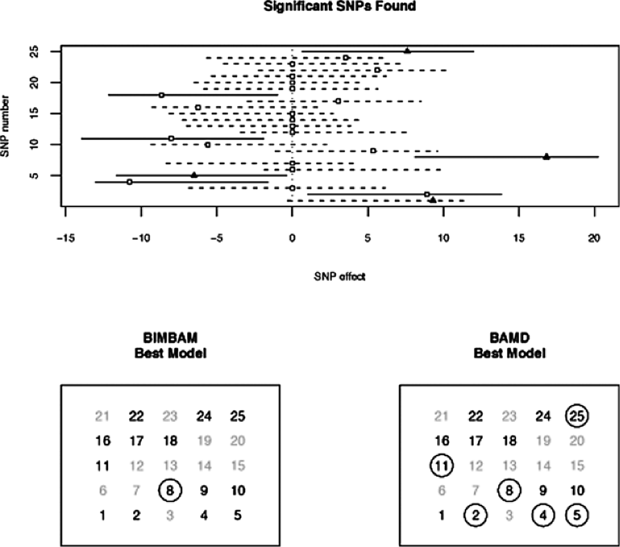
The results for each comparison are summarized through two diagrams. The first (the upper panels in Figures 1 and 2) display the SNPs that BAMD and BIMBAM found to be significant in the first stage. The lower panels in Figures 1 and 2 display the output from the variable selection procedure.
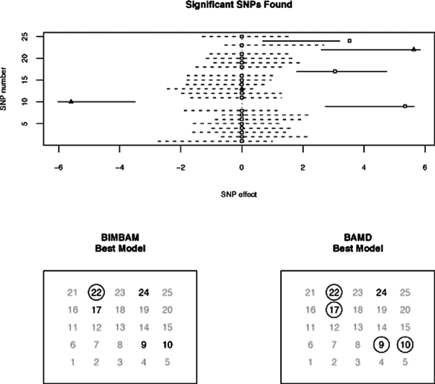
Each figure shows that BAMD significantly outperforms BIMBAM. In the first example, BIMBAM found only one of the significant SNPs, while BAMD found six. In the second example, there were five significant SNPs, and BIMBAM only found one again, while BAMD found four of them.
5 Analysis of the loblolly pine data
Carbon isotope discrimination (CID) is a time-integrated trait measure of water use efficiency. González-Martínez et al. (2008) used the family-based approach of the Quantitative Transmission Disequilibrium Test QTDT to detect SNPs associated with CID. We utilized the family structure of this population [also described in Kayihan et al. (2005)] in the design matrix in our model. Of the 61 control-pollinated families measured for CID, each had approximately 15 offspring that were clonally propagated by rooted cuttings to generate the ramets (genetically identical replicates). Each genotype has two ramets, sampled from each of two testing sites at Cuthbert, GA and Palatka, FL. Our approach enables us to utilize the family pedigree and parental information to recover missing SNP genotypes. With informative priors, we infer the progeny SNP genotype through Mendelian randomization [Falconer and Macay (1996)]. With uninformative priors, we assume SNPs are missing at random and assign equal probability for each genotype class for missing SNPs.
All SNPs are simultaneously tested under our association model. The Gibbs sampler ran for 50,000 iterations. The first 10,000 iterations were burn-in, after which we thinned the chain every 4 iterations; the autocorrelation reduced significantly after thinning (data not shown). Thus, we have a total of 10,000 samples for each chain for our statistics, and we then applied the variable selector on the four SNPs that were found when using the informative prior.
| SNP | |||
| Informative prior | Uninformative prior | ||
| 95% C.I. | 95% C.I. | Type | |
| (3) caf1_s1∗ | (0.008, 0.110) | (0.013, 0.129) | Syn |
| (5) ccoaomt_s10∗† | (0.103, 0.012) | (0.097, 0.005) | NC(intron) |
| (6) cpk3_s5 | (0.052, 0.004) | (0.048, 0.001) | Syn |
| (29) dhn1_s2∗† | (0.065, 0.113) | (0.044, 0.092) | NC(UTR) |
| (31) ein2_s1∗† | (0.077, 0.142) | (0.067, 0.126) | NC(UTR) |
[]∗ Indicates significant in González-Martínez et al. (2008). Bold type indicates significant at the 5% level from our association testing, the rest being nonsignificant. † indicates presence in best model found by variable selector. As indicated in González-Martínez et al. (2008), there are additional SNPs that are marginally significant at , which we also detected. ‡: Syn, synonymous SNP; NC, noncoding; UTR, untranslated region.
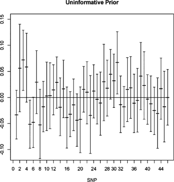
We detected significant effects of several SNPs on CID at a 95% Bayesian confidence interval (Table 4). Using the uninformative prior, we found 3 significant SNPs [(3) ccoaomt_s10, (5) ein2_s1, (31) Caf1_s1]. Using the informative prior, we detected 4 SNPs [(5) ein2_s1, (6) cpk3_s5, (29) dhn1_s2, (31) Caf1_s1] as significant. Note that (6) and (29) are close to significant using the uninformative prior, and (3) was close to significant using the informative prior. This suggests that for these data, the effect of the prior information is important. The QTDT test resulted in 4 significant SNPs, (3), (5), (29), (31), all of which were detected by BAMD which, in addition, found SNP (6). Moreover, it is important to note that BAMD detected these SNPs simultaneously, an indication that their collective effect on the phenotype is being detected.
The use of tag SNPs in a pedigree does not allow for “fine mapping” to SNP effects [Neale and Ingvarsson (2008), Flint-Garcia, Thornsberry and Buckler (2003)]. Thus, the effects of these SNPs on carbon isotope discrimination may reflect the involvement of many linked genes on the phenotype.
We also provide Figures 3 and 4, showing the results for all of the SNPs in the data set. Figure 3 is based on using uninformative SNP priors, while Figure 4 uses informative priors. Although there are few differences in the graphs (showing the strength of the data with respect to the model), we see that the prior can matter. For example, SNP (3) is significant when the noninformative prior is used, but not so when we use the informative prior. The opposite finding holds for SNP (6). Looking at the figures, we see that the significant intervals only barely cross zero; thus, the inclusion of relevant prior information can be quite important.
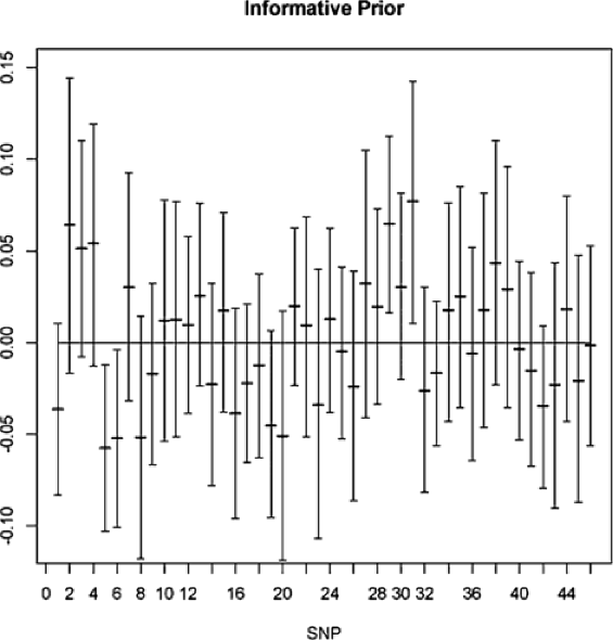
The four SNPs picked out when using the informative prior were (5), (6), (29), and (31). Due to the small number of variables under consideration, the variable selector procedure was able to run through all 16 possible models. The one with the highest Bayes factor was found to contain SNPs (5), (29), and (31).
6 Discussion
Association testing is being applied to discover relationships among SNPs and complex traits in plants and animals [Flint-Garcia, Thornsberry and Buckler (2003), Hirschhorn and Daly (2005), Balding (2006), Zhu et al. (2008)]. Our model was developed specifically for detecting associations in loblolly pine data, but can be applied to other species as well. Here we discuss some features and limitations of the method.
Multiple imputation
Multiple imputation of missing SNP data is the best way to ensure unbiased parameter estimates, which is an important consideration given that SNP effects tend to be small for complex traits of greatest biological interest, and given that results of association studies typically motivate more detailed and labor-intensive investigations of how and why associations were detected.
We used simulation to compare BAMD and BIMBAM for their detection of “correct” vs. “incorrect” SNPs, and found that BAMD performed better than BIMBAM. In practice, this advantage of BAMD over BIMBAM would likely be greatest when missing SNPs are not in LD with nearby SNPs (or adjacency cannot be determined). This is the case in many species, including loblolly pine, in which LD is low and genomic resources such as high-resolution genomic maps and high-density SNP chips for genome scanning are not as well developed as they are for the human genome. The higher computational intensity required for formal multiple imputation in BAMD is a trade-off, however, this has not restricted its practical use in most data sets. For very large data sets, parallel processing seems a logical next step in further increasing the computational efficiency of BAMD.
Family structure
Our method can be applied to family-based association populations, populations of unrelated genotypes, or combination populations. It can incorporate prior information if known. [The application of BAMD in Quesada et al. (2010) was to a population of unrelated genotypes, where significant SNPs related to disease resistance were found.]
Probit models
Although here we assume a continuous response variable, the method can be adapted to discrete phenotypes using a probit link. For example, in a case control study, the response would be either case or control status, and with a probit model we add a latent variable in the Gibbs sampler.
SNP detection
Although BAMD successfully detected the same significant SNPs as were previously detected using the family-based method QTDT [González-Martínez et al. (2008)], as well as an additional significant SNP, the BAMD variable selector indicated that a subset of the significant SNPs was sufficient to explain variation in the phenotype carbon isotope discrimination. This is a useful tool for biologists because a simultaneous solution for SNP effects enables detection of numerous SNPs that collectively explain phenotypes, which in turn enables further biological experiments to investigate their underlying basis.
However, the candidate SNPs found by BAMD and QTDT cannot necessarily be deemed “correct” or “incorrect” without additional biological experiments. As such, little more can be stated about the correctness of SNPs 3, 5, 29, and 31 without validation experiments. In the broader context of association testing, it is relevant to note that the use of QTDT is limited to families, whereas BAMD and BIMBAM can be used to detect associations in families as well as populations of unrelated individuals. The ability to use BAMD and BIMBAM in many different types of populations is appealing.
Simultaneous vs. genome-wide
Genome-wide association studies are, typically, marginal processors of the data. That is, each SNP is assessed individually for its association, so simultaneous assessment, or epistasis, cannot be detected. A model such as (1) is assessing the SNPs simultaneously—that is its strength. But how many SNPs should we expect to be able to handle in one model? Computational issues aside, if the number of SNPs is greatly increased, we are then susceptible to the usual regression pitfalls—multicollinearity being the most prevalent. Thus, we recommend using BAMD on smaller sets of SNPs that have had some preprocessing. Thus far, BAMD has been used successfully on a model with SNPs [Quesada et al. (2010)], and we have tested it on as many as SNPs.
Missing data
The missing data problem is common across all genomics data sets, so there is broad potential utility of this method. The assumption of MAR (missing at random), which is reasonable in these contexts, may bear additional research attention. If there are quality concerns about SNP data, there are some statistical steps forward, as noted by Wilson et al. (2010), such as using indicator variables of missingness as predictors. This approach can even be extended to test if missingness is a heritable trait and, if so, the MAR assumption is invalid. Next generation sequencing platforms may generate sufficient data to enable this assumption to be tested and, if borne out, may motivate placement of priors on SNP calls in certain sequence contexts.
Last, software to run the Gibbs sampler and variable selector is available in the R package BAMD.
Appendix A Calculating the numerator relationship matrix
The algorithm is due to Henderson (1976) and Quaas (1976). The individuals within families and the parents for the families are ordered together such that the first subjects are unrelated and are used as a “base” population. Let the total number of subjects within families and parents of the families be , and we will get a numerator relationship matrix with dimension . As the first subjects (being part of the parents of the families ) are unrelated, the upper left submatrix with dimension of the numerator relationship matrix is identity matrix . This identity submatrix will be expanded iteratively until it reaches to dimension .
As we know the sub-numerator relationship matrix for the first unrelated subjects is the identity, next we will give the details how to calculate the remaining cells of the numerator relationship matrix for the related subjects. Consider the th and the th subject from the above ordered subjects: {longlist}[(2)]
If both parents of the th individual are known, say, and , then
where is the cell of the numerator relationship matrix in the th row and th column.
If only one parent is known for the th subject, say, it is , then
If neither parent is known for the th subject,
For the loblolly pine data, we have pines acting as grandparents and they produce pine families. The families contains individual pine trees all together, also called clones. The phenotypic responses are taken from the individual clones. So our interest is in calculating the relationship matrix for the clones and it would have a dimension . According to Henderson’s method, we ordered the grandparent pines and individual pines together such that the first pines are not related. Starting from the th pine, we applied the above iteration calculation algorithm, and in the end had a relationship matrix with dimension for all the grandparent pines and all individual clones. We took a submatrix from the right bottom of the previous numerator relationship matrix with dimension and it is the numerator relationship matrix we used in the loblolly pine data analysis.
Appendix B Estimation with the EM algorithm
B.1 Missing data
The EM algorithm begins by building the complete data likelihood, which is the likelihood function that would be used if the missing data were observed. When we fill in the missing data we write , and the complete data are with likelihood function
where indexes those individuals with complete SNP data, and indexes those individuals with missing SNP information.
The observed data likelihood, which is the function that we eventually use to estimate the parameters, must be summed over all possible values of the missing data. So we have
The distribution of the missing data is given by the ratio of :
| (12) |
where the sum in the denominator is over all possible realizations of . This is a discrete distribution on the missing SNP data for each individual. To understand it, look at one individual.
Suppose that there are possible genotypes (typically or ) and individual has missing data on SNPs. So the data for individual is , where has elements, each of which could be one of classes. For example, if and , then can take values in the following:
| SNP | |||||||
|---|---|---|---|---|---|---|---|
| Genotype | |||||||
where the show one possible value of the . For the example, there are possible values for . In a real data set this could grow out of hand. For example, if there were missing SNPs, then there are 531,441 possible values for ; with 20 missing SNPs the number grows to 3,486,784,401 (3.5 billion).
B.2 An EM algorithm
To the expected value of the log of the complete data likelihood (B.1), we only deal with the second term (with the missing data). This expected value does not change the piece with no missing data, but does change the second piece. Standard calculations give
where
| (13) |
If we define
the expected complete data log likelihood is
| (14) |
where is the variance–covariance matrix of the vector with elements given by
and . Standard calculus will show that the MLEs from (14) are given by
| (15) | |||||
The algorithm now iterates between (12), (13), and (B.2) until convergence.
B.3 Implementation
To implement the EM algorithm, we must be able to either: {longlist}[(1)]
calculate the expectation and variance in (13), or
generate a random sample from (12) and calculate the terms in (13) by simulation. The first option is impossible and the second is computationally intensive, but the only way.
Going back to (12), note that this is the distribution of the vector of missing values for individual . If the data are , we are only concerned with , and for ,
where the sum in the denominator can easily have over billion terms.
A possible alternative is to use a Gibbs sampler to simulate the distribution of by calculating the distribution of each element conditional on the rest of the vector. For a particular element , the conditional distribution given the rest of the vector is given in (2.2). So to produce a sample of , we loop through a Gibbs sampler.
Unfortunately, there may be problems with this algorithm in that it may still be too computationally intensive. The Gibbs samplers (2.2) and (2.2) need to be run for every iteration of the EM algorithm. For each iteration of EM we may need 20–50 thousand Gibbs iterations. If there is a lot of missing data, this could result in a very slow algorithm.
Appendix C Matrix inverse updates
We are interested in matrices of the form , where , , are vectors. For this form we have the following lemma, which follows from Woodbury’s formula.
Lemma 1
Let be invertible, and , , be vectors. Define
Then for ,
| (16) |
Then, to calculate , we can start with , and use the recursion to get to . Note that each step of the recursion requires only multiplication of matrices by vectors. Moreover, in many applications the vectors are sparse, so the multiplication amounts to extracting elements.
[id=suppA] \stitleTheory and additional simulations \slink[doi]10.1214/11-AOAS516SUPP \slink[url]http://lib.stat.cmu.edu/aoas/516/supplement.pdf \sdatatype.pdf \sdescriptionThe Supplemental Information contains details on the variable selector, and the proof of convergence of the two Markov chains (the Gibbs sampler and the model search). In addition, there are further comparisons between BAMD and BIMBAM.
References
- Balding (2006) {barticle}[pbm] \bauthor\bsnmBalding, \bfnmDavid J.\binitsD. J. (\byear2006). \btitleA tutorial on statistical methods for population association studies. \bjournalNat. Rev. Genet. \bvolume7 \bpages781–791. \biddoi=10.1038/nrg1916, issn=1471-0056, pii=nrg1916, pmid=16983374 \bptokimsref \endbibitem
- Casella et al. (2009) {barticle}[mr] \bauthor\bsnmCasella, \bfnmGeorge\binitsG., \bauthor\bsnmGirón, \bfnmF. Javier\binitsF. J., \bauthor\bsnmMartínez, \bfnmM. Lina\binitsM. L. and \bauthor\bsnmMoreno, \bfnmElías\binitsE. (\byear2009). \btitleConsistency of Bayesian procedures for variable selection. \bjournalAnn. Statist. \bvolume37 \bpages1207–1228. \biddoi=10.1214/08-AOS606, issn=0090-5364, mr=2509072 \bptokimsref \endbibitem
- Chen and Abecasis (2007) {barticle}[auto:STB—2012/01/05—16:28:07] \bauthor\bsnmChen, \bfnmW. M.\binitsW. M. and \bauthor\bsnmAbecasis, \bfnmG. R.\binitsG. R. (\byear2007). \btitleFamily-based association tests for genomewide association scan. \bjournalThe American Journal of Human Genetics \bvolume81 \bpages913–926. \bptokimsref \endbibitem
- Chen and Shao (1997) {barticle}[mr] \bauthor\bsnmChen, \bfnmMing-Hui\binitsM.-H. and \bauthor\bsnmShao, \bfnmQi-Man\binitsQ.-M. (\byear1997). \btitleEstimating ratios of normalizing constants for densities with different dimensions. \bjournalStatist. Sinica \bvolume7 \bpages607–630. \bidissn=1017-0405, mr=1467451 \bptokimsref \endbibitem
- Dai et al. (2006) {barticle}[pbm] \bauthor\bsnmDai, \bfnmJames Y.\binitsJ. Y., \bauthor\bsnmRuczinski, \bfnmIngo\binitsI., \bauthor\bsnmLeBlanc, \bfnmMichael\binitsM. and \bauthor\bsnmKooperberg, \bfnmCharles\binitsC. (\byear2006). \btitleImputation methods to improve inference in SNP association studies. \bjournalGenet. Epidemiol. \bvolume30 \bpages690–702. \biddoi=10.1002/gepi.20180, issn=0741-0395, pmid=16986162 \bptokimsref \endbibitem
- Falconer and Macay (1996) {bbook}[auto:STB—2012/01/05—16:28:07] \bauthor\bsnmFalconer, \bfnmD. S.\binitsD. S. and \bauthor\bsnmMacay, \bfnmT. F. C.\binitsT. F. C. (\byear1996). \btitleIntroduction to Quantitative Genetics, \bedition4th ed. \bpublisherLongman, \baddressHarlow. \bptokimsref \endbibitem
- Flint-Garcia, Thornsberry and Buckler (2003) {barticle}[auto:STB—2012/01/05—16:28:07] \bauthor\bsnmFlint-Garcia, \bfnmS. A.\binitsS. A., \bauthor\bsnmThornsberry, \bfnmJ. M.\binitsJ. M. and \bauthor\bsnmBuckler, \bfnmE. S.\binitsE. S. (\byear2003). \btitleStructure of linkage disequilibrium in plants. \bjournalAnnu. Rev. Plant Bio. \bvolume54 \bpages357–374. \bptokimsref \endbibitem
- González-Martínez et al. (2006) {barticle}[auto:STB—2012/01/05—16:28:07] \bauthor\bsnmGonzález-Martínez, \bfnmS. C.\binitsS. C., \bauthor\bsnmErsoz, \bfnmE.\binitsE., \bauthor\bsnmBrown, \bfnmG. R.\binitsG. R., \bauthor\bsnmWheeler, \bfnmN. C.\binitsN. C. and \bauthor\bsnmNeale, \bfnmD. B.\binitsD. B. (\byear2006). \btitleDNA sequence variation and selection of tag single-nucleotide polymorphisms at candidate genes for drought-stress response in Pinus taeda L. \bjournalGenetics \bvolume172 \bpages1915–1926. \bptokimsref \endbibitem
- González-Martínez et al. (2008) {barticle}[auto:STB—2012/01/05—16:28:07] \bauthor\bsnmGonzález-Martínez, \bfnmS. C.\binitsS. C., \bauthor\bsnmHuber, \bfnmD. A.\binitsD. A., \bauthor\bsnmErsoz, \bfnmE.\binitsE., \bauthor\bsnmDavis, \bfnmJ. M.\binitsJ. M. and \bauthor\bsnmNeale, \bfnmD. B.\binitsD. B. (\byear2008). \btitleAssociation genetics in Pinus taeda L. II. Carbon isotope discrimination. \bjournalHeredity \bvolume101 \bpages19–26. \bptokimsref \endbibitem
- Greenland and Finkle (1995) {barticle}[auto:STB—2012/01/05—16:28:07] \bauthor\bsnmGreenland, \bfnmS.\binitsS. and \bauthor\bsnmFinkle, \bfnmW. D.\binitsW. D. (\byear1995). \btitleA critical look at methods for handling missing covariates in epidemiologic regression analyses. \bjournalAm. J. Epidemiol. \bvolume142 \bpages1255–1264. \bptokimsref \endbibitem
- Hager (1989) {barticle}[mr] \bauthor\bsnmHager, \bfnmWilliam W.\binitsW. W. (\byear1989). \btitleUpdating the inverse of a matrix. \bjournalSIAM Rev. \bvolume31 \bpages221–239. \biddoi=10.1137/1031049, issn=0036-1445, mr=0997457 \bptokimsref \endbibitem
- Henderson (1976) {barticle}[auto:STB—2012/01/05—16:28:07] \bauthor\bsnmHenderson, \bfnmC. R.\binitsC. R. (\byear1976). \btitleA simple method for computing the inverse of a numerator relationship matrix used in prediction of breeding values. \bjournalBiometrics \bvolume32 \bpages69–83. \bptokimsref \endbibitem
- Hirschhorn and Daly (2005) {barticle}[auto:STB—2012/01/05—16:28:07] \bauthor\bsnmHirschhorn, \bfnmJ. N.\binitsJ. N. and \bauthor\bsnmDaly, \bfnmM. J.\binitsM. J. (\byear2005). \btitleGenome-wide association studies for common diseases and complex traits. \bjournalNature Genetics \bvolume6 \bpages95–108. \bptokimsref \endbibitem
- Hobert and Casella (1996) {barticle}[mr] \bauthor\bsnmHobert, \bfnmJames P.\binitsJ. P. and \bauthor\bsnmCasella, \bfnmGeorge\binitsG. (\byear1996). \btitleThe effect of improper priors on Gibbs sampling in hierarchical linear mixed models. \bjournalJ. Amer. Statist. Assoc. \bvolume91 \bpages1461–1473. \bidissn=0162-1459, mr=1439086 \bptokimsref \endbibitem
- Huisman (2000) {barticle}[auto:STB—2012/01/05—16:28:07] \bauthor\bsnmHuisman, \bfnmM.\binitsM. (\byear2000). \btitleImputation of missing item responses: Some simple techniques. \bjournalQuality and Quantity \bvolume34 \bpages331–351. \bptokimsref \endbibitem
- Kayihan et al. (2005) {barticle}[auto:STB—2012/01/05—16:28:07] \bauthor\bsnmKayihan, \bfnmG. C.\binitsG. C., \bauthor\bsnmHuber, \bfnmD. A.\binitsD. A., \bauthor\bsnmMorse, \bfnmA. M.\binitsA. M., \bauthor\bsnmWhite, \bfnmT. T.\binitsT. T. and \bauthor\bsnmDavis, \bfnmJ. M.\binitsJ. M. (\byear2005). \btitleGenetic dissection of fusiform rust and pitch canker disease traits in loblolly pine. \bjournalTheory of Applied Genetics \bvolume110 \bpages948–958. \bptokimsref \endbibitem
- Li et al. (2011) {bmisc}[auto:STB—2012/01/09—08:49:38] \bauthor\bsnmLi, \bfnmZhen\binitsZ., \bauthor\bsnmGopal, \bfnmVikneswaran\binitsV., \bauthor\bsnmLi, \bfnmXiaobo\binitsX., \bauthor\bsnmDavis, \bfnmJohn M.\binitsJ. M. and \bauthor\bsnmCasella, \bfnmGeorge\binitsG. (\byear2011). \bhowpublishedSupplement to “Simultaneous SNP identification in association studies with missing data.” DOI:\doiurl10.1214/11-AOAS516SUPP. \bptokimsref \endbibitem
- Little and Rubin (2002) {bbook}[mr] \bauthor\bsnmLittle, \bfnmRoderick J. A.\binitsR. J. A. and \bauthor\bsnmRubin, \bfnmDonald B.\binitsD. B. (\byear2002). \btitleStatistical Analysis with Missing Data. \bpublisherWiley, \baddressNew York. \bptokimsref \endbibitem
- Marchini et al. (2007) {barticle}[pbm] \bauthor\bsnmMarchini, \bfnmJonathan\binitsJ., \bauthor\bsnmHowie, \bfnmBryan\binitsB., \bauthor\bsnmMyers, \bfnmSimon\binitsS., \bauthor\bsnmMcVean, \bfnmGil\binitsG. and \bauthor\bsnmDonnelly, \bfnmPeter\binitsP. (\byear2007). \btitleA new multipoint method for genome-wide association studies by imputation of genotypes. \bjournalNat. Genet. \bvolume39 \bpages906–913. \biddoi=10.1038/ng2088, issn=1061-4036, pii=ng2088, pmid=17572673 \bptokimsref \endbibitem
- McKeever and Howard (1996) {barticle}[auto:STB—2012/01/05—16:28:07] \bauthor\bsnmMcKeever, \bfnmD. B.\binitsD. B. and \bauthor\bsnmHoward, \bfnmJ. L.\binitsJ. L. (\byear1996). \btitleValue of timber and agricultural products in the United States 1991. \bjournalForest Products Journal \bvolume46 \bpages45–50. \bptokimsref \endbibitem
- Meng and Wong (1996) {barticle}[mr] \bauthor\bsnmMeng, \bfnmXiao-Li\binitsX.-L. and \bauthor\bsnmWong, \bfnmWing Hung\binitsW. H. (\byear1996). \btitleSimulating ratios of normalizing constants via a simple identity: A theoretical exploration. \bjournalStatist. Sinica \bvolume6 \bpages831–860. \bidissn=1017-0405, mr=1422406 \bptokimsref \endbibitem
- Neale and Ingvarsson (2008) {barticle}[pbm] \bauthor\bsnmNeale, \bfnmDavid B.\binitsD. B. and \bauthor\bsnmIngvarsson, \bfnmPär K.\binitsP. K. (\byear2008). \btitlePopulation, quantitative and comparative genomics of adaptation in forest trees. \bjournalCurr. Opin. Plant Biol. \bvolume11 \bpages149–155. \biddoi=10.1016/j.pbi.2007.12.004, issn=1369-5266, pii=S1369-5266(07)00177-X, pmid=18262830 \bptokimsref \endbibitem
- O’Hagan and Forster (2004) {bbook}[auto:STB—2012/01/05—16:28:07] \bauthor\bsnmO’Hagan, \bfnmA.\binitsA. and \bauthor\bsnmForster, \bfnmJ.\binitsJ. (\byear2004). \btitleKendall’s Advanced Theory of Statistics: Vol. 2B: Bayesian Inference. \bpublisherArnold, \baddressLondon. \bptokimsref \endbibitem
- Pritchard, Stephens and Donnelly (2000) {barticle}[pbm] \bauthor\bsnmPritchard, \bfnmJ. K.\binitsJ. K., \bauthor\bsnmStephens, \bfnmM.\binitsM. and \bauthor\bsnmDonnelly, \bfnmP.\binitsP. (\byear2000). \btitleInference of population structure using multilocus genotype data. \bjournalGenetics \bvolume155 \bpages945–959. \bidissn=0016-6731, pmcid=1461096, pmid=10835412 \bptokimsref \endbibitem
- Quaas (1976) {barticle}[auto:STB—2012/01/05—16:28:07] \bauthor\bsnmQuaas, \bfnmR. L.\binitsR. L. (\byear1976). \btitleComputing the diagonal elements and inverse of a large numerator relationship matrix. \bjournalBiometrics \bvolume46 \bpages949–953. \bptokimsref \endbibitem
- Quesada et al. (2010) {barticle}[auto:STB—2012/01/05—16:28:07] \bauthor\bsnmQuesada, \bfnmT.\binitsT., \bauthor\bsnmGopal, \bfnmV.\binitsV., \bauthor\bsnmCumbie, \bfnmW. P.\binitsW. P., \bauthor\bsnmEckert, \bfnmA. J.\binitsA. J., \bauthor\bsnmWegrzyn, \bfnmJ. L.\binitsJ. L., \bauthor\bsnmNeale, \bfnmD. B.\binitsD. B., \bauthor\bsnmGoldfarb, \bfnmB.\binitsB., \bauthor\bsnmHuber, \bfnmD. A.\binitsD. A., \bauthor\bsnmCasella, \bfnmG.\binitsG. and \bauthor\bsnmDavis, \bfnmJ. M.\binitsJ. M. (\byear2010). \btitleAssociation mapping of quantitative disease resistance in a natural population of Loblolly pine (Pinus taeda L.). \bjournalGenetics \bvolume186 \bpages677–686. \bptokimsref \endbibitem
- Scheet and Stephens (2006) {barticle}[auto:STB—2012/01/05—16:28:07] \bauthor\bsnmScheet, \bfnmP.\binitsP. and \bauthor\bsnmStephens, \bfnmM. A.\binitsM. A. (\byear2006). \btitleA fast and flexible statistical model for large-scale population genotype data: Applications to inferring missing genotypes and haplotypic phase. \bjournalAm. Journ. Hum. Genetics \bvolume78 \bpages629–644. \bptokimsref \endbibitem
- Servin and Stephens (2007) {barticle}[auto:STB—2012/01/05—16:28:07] \bauthor\bsnmServin, \bfnmB.\binitsB. and \bauthor\bsnmStephens, \bfnmM.\binitsM. (\byear2007). \btitleImputation-based analysis of association studies: Candidate regions and quantitative traits. \bjournalPLoS Genet. \bvolume3 \bpagese114. \biddoi=10.1371/journal.pgen.0030114 \bptokimsref \endbibitem
- Stephens, Smith and Donnelly (2001) {barticle}[pbm] \bauthor\bsnmStephens, \bfnmM.\binitsM., \bauthor\bsnmSmith, \bfnmN. J.\binitsN. J. and \bauthor\bsnmDonnelly, \bfnmP.\binitsP. (\byear2001). \btitleA new statistical method for haplotype reconstruction from population data. \bjournalAm. J. Hum. Genet. \bvolume68 \bpages978–989. \biddoi=10.1086/319501, issn=0002-9297, pii=S0002-9297(07)61424-4, pmcid=1275651, pmid=11254454 \bptokimsref \endbibitem
- Su et al. (2008) {barticle}[auto:STB—2012/01/05—16:28:07] \bauthor\bsnmSu, \bfnmS. Y.\binitsS. Y., \bauthor\bsnmWhite, \bfnmJ.\binitsJ., \bauthor\bsnmBalding, \bfnmD. J.\binitsD. J. and \bauthor\bsnmCoin, \bfnmL. J. M.\binitsL. J. M. (\byear2008). \btitleInference of haplotypic phase and missing genotypes in polyploid organisms and variable copy number genomic regions. \bjournalBMC Bioinformatics \bvolume9 \bpagesArt. 513. \bptokimsref \endbibitem
- Sun and Kardia (2008) {barticle}[auto:STB—2012/01/05—16:28:07] \bauthor\bsnmSun, \bfnmY. V.\binitsY. V. and \bauthor\bsnmKardia, \bfnmS. L. R.\binitsS. L. R. (\byear2008). \btitleImputing missing genotypic data of single-nucleotide polymorphisms using neural networks. \bjournalEuropean Journal of Human Genetics \bvolume16 \bpages487–495. \bptokimsref \endbibitem
- Szatkiewicz et al. (2008) {barticle}[auto:STB—2012/01/05—16:28:07] \bauthor\bsnmSzatkiewicz, \bfnmJ. P.\binitsJ. P., \bauthor\bsnmBeane, \bfnmG. L.\binitsG. L., \bauthor\bsnmDing, \bfnmY.\binitsY., \bauthor\bsnmHutchins, \bfnmL.\binitsL., \bauthor\bparticlede \bsnmVillena, \bfnmF. P.\binitsF. P. and \bauthor\bsnmChurchill, \bfnmG. A.\binitsG. A. (\byear2008). \btitleAn imputed genotype resource for the laboratory mouse. \bjournalMammalian Genome \bvolume19 \bpages199–208. \bptokimsref \endbibitem
- van der Heijden et al. (2006) {barticle}[pbm] \bauthor\bparticlevan der \bsnmHeijden, \bfnmGeert J.\binitsG. J., \bauthor\bsnmDonders, \bfnmA. Rogier\binitsA. R., \bauthor\bsnmStijnen, \bfnmTheo\binitsT. and \bauthor\bsnmMoons, \bfnmKarel G.\binitsK. G. (\byear2006). \btitleImputation of missing values is superior to complete case analysis and the missing-indicator method in multivariable diagnostic research: A clinical example. \bjournalJ. Clin. Epidemiol. \bvolume59 \bpages1102–1109. \biddoi=10.1016/j.jclinepi.2006.01.015, issn=0895-4356, pii=S0895-4356(06)00198-3, pmid=16980151 \bptokimsref \endbibitem
- Wear and Greis (2002) {barticle}[auto:STB—2012/01/05—16:28:07] \bauthor\bsnmWear, \bfnmD. N.\binitsD. N. and \bauthor\bsnmGreis, \bfnmJ. G.\binitsJ. G. (\byear2002). \btitleSouthern forest resource assessment: Summary of findings. \bjournalJournal of Forestry \bvolume100 \bpages6–14. \bptokimsref \endbibitem
- Wilson et al. (2010) {barticle}[mr] \bauthor\bsnmWilson, \bfnmMelanie A.\binitsM. A., \bauthor\bsnmIversen, \bfnmEdwin S.\binitsE. S., \bauthor\bsnmClyde, \bfnmMerlise A.\binitsM. A., \bauthor\bsnmSchmidler, \bfnmScott C.\binitsS. C. and \bauthor\bsnmSchildkraut, \bfnmJoellen M.\binitsJ. M. (\byear2010). \btitleBayesian model search and multilevel inference for SNP association studies. \bjournalAnn. Appl. Stat. \bvolume4 \bpages1342–1364. \biddoi=10.1214/09-AOAS322, issn=1932-6157, mr=2758331 \bptokimsref \endbibitem
- Yu et al. (2006) {barticle}[auto:STB—2012/01/05—16:28:07] \bauthor\bsnmYu, \bfnmJ. M.\binitsJ. M., \bauthor\bsnmPressoir, \bfnmG.\binitsG., \bauthor\bsnmBriggs, \bfnmW. H.\binitsW. H., \bauthor\bsnmBi, \bfnmI. V.\binitsI. V., \bauthor\bsnmYamasaki, \bfnmM.\binitsM., \bauthor\bsnmDoebley, \bfnmJ.\binitsJ., \bauthor\bsnmMcMullen, \bfnmM. D.\binitsM. D., \bauthor\bsnmGaut, \bfnmB. S.\binitsB. S., \bauthor\bsnmNielsen, \bfnmD. M.\binitsD. M., \bauthor\bsnmHolland, \bfnmJ. B.\binitsJ. B., \bauthor\bsnmKresovich, \bfnmS.\binitsS. and \bauthor\bsnmBuckler, \bfnmE. S.\binitsE. S. (\byear2006). \btitleA unified mixed model method for association mapping that accounts for multiple levels of relatedness. \bjournalNature Genetics \bvolume38 \bpages203–208. \bptokimsref \endbibitem
- Zhu et al. (2008) {barticle}[auto:STB—2012/01/05—16:28:07] \bauthor\bsnmZhu, \bfnmC.\binitsC., \bauthor\bsnmGore, \bfnmM.\binitsM., \bauthor\bsnmBuckler, \bfnmE. S.\binitsE. S. and \bauthor\bsnmYu, \bfnmJ.\binitsJ. (\byear2008). \btitleStatus and prospects of association mapping in plants. \bjournalThe Plant Genome \bvolume1 \bpages5–20. \bptokimsref \endbibitem