Single Image Deraining with Continuous Rain Density Estimation
Abstract
Single image deraining (SIDR) often suffers from over/under deraining due to the nonuniformity of rain densities and the variety of raindrop scales. In this paper, we propose a continuous density guided network (CODE-Net) for SIDR. Particularly, it is composed of a rain streak extractor and a denoiser, where the convolutional sparse coding (CSC) is exploited to filter out noises from the extracted rain streaks. Inspired by the reweighted iterative soft-threshold for CSC, we address the problem of continuous rain density estimation by learning the weights with channel attention blocks from sparse codes. We further develop a multiscale strategy to depict rain streaks appearing at different scales. Experiments on synthetic and real-world data demonstrate the superiority of our methods over recent state of the arts, in terms of both quantitative and qualitative results. Additionally, instead of quantizing rain density with several levels, our CODE-Net can provide continuous-valued estimations of rain densities, which is more desirable in real applications.
Index Terms:
Image deraining, rain density estimation, convolutional sparse coding.I Introduction
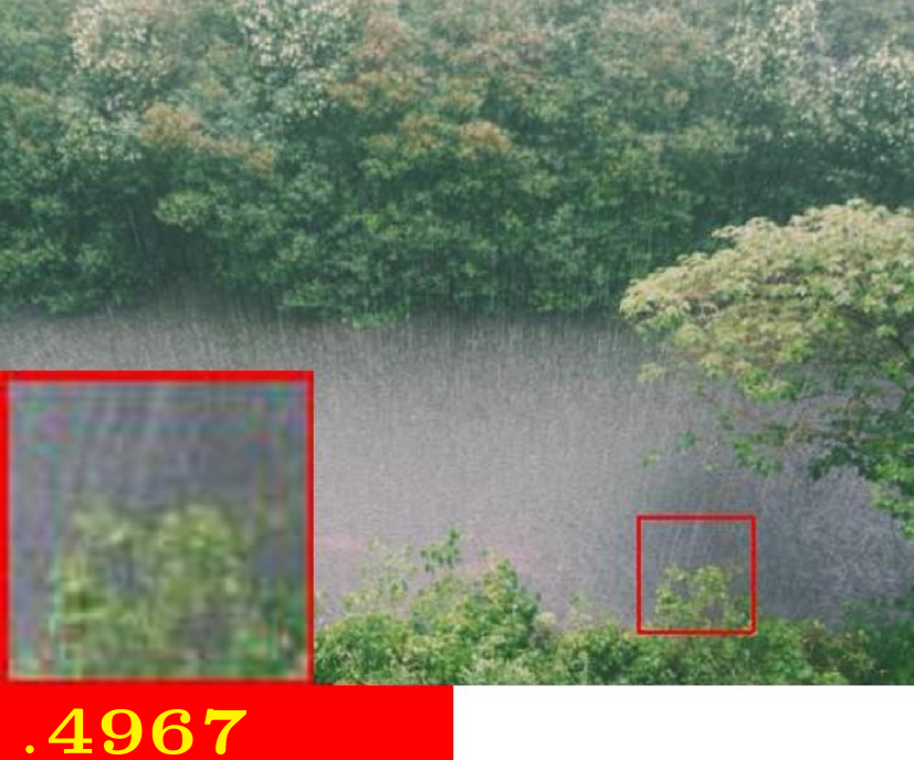
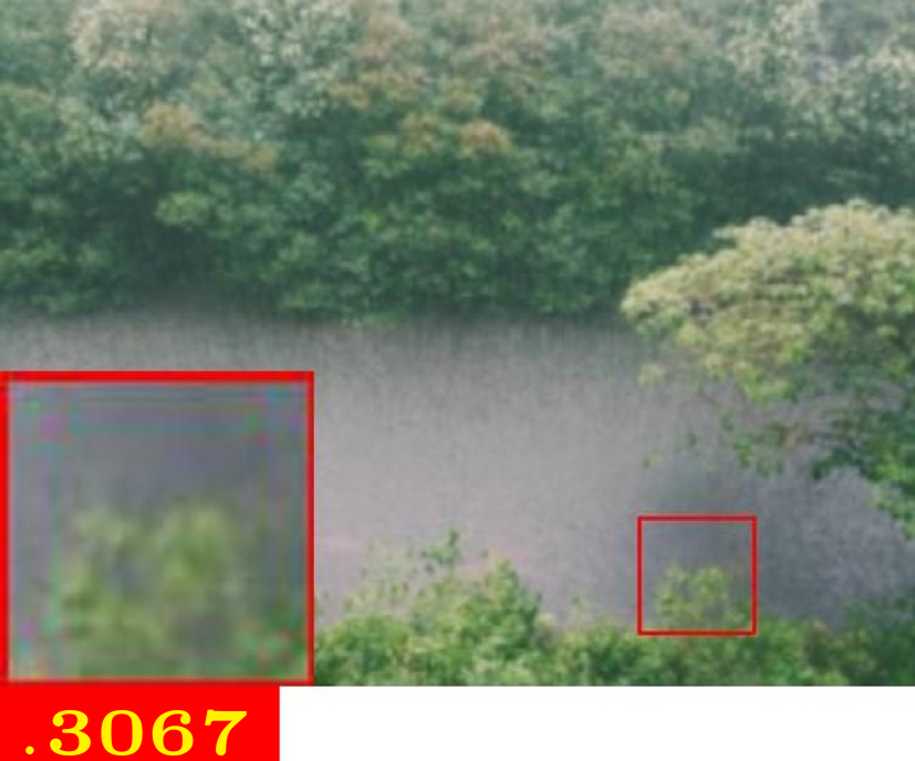
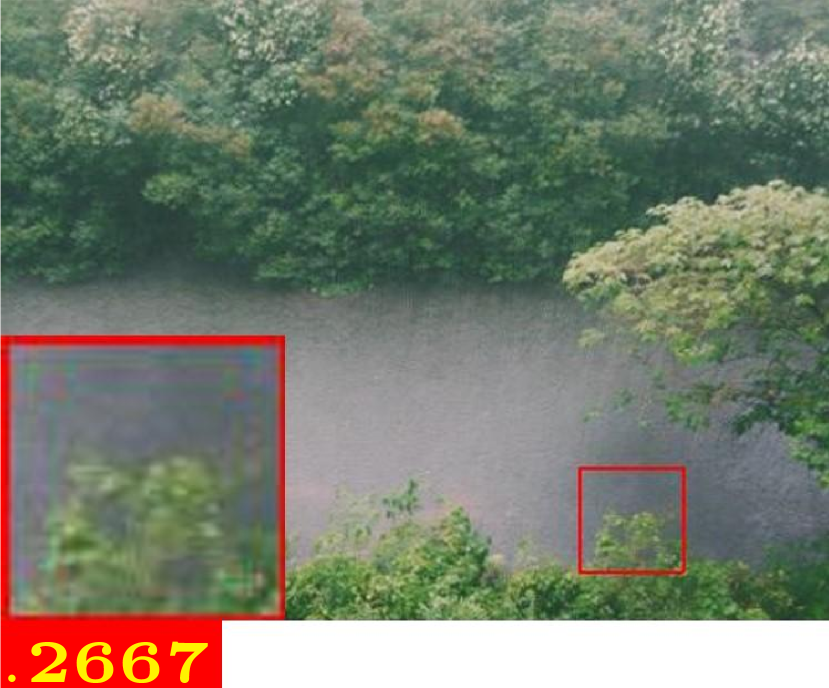
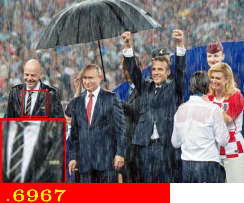
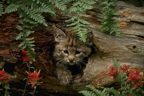
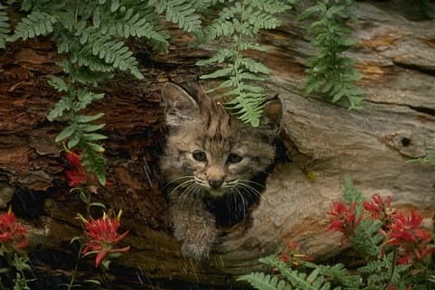
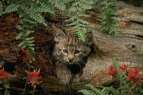
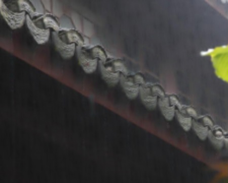
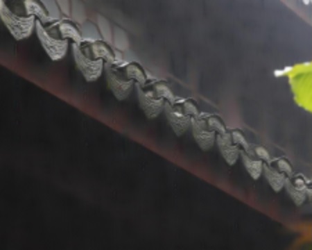
Images captured in rainy weather are often severely contaminated by rain streaks, which may largely degrade the performance of the outdoor vision systems. Image deraining is to remove rain streaks from rainy images and many approaches have been proposed either by adopting priors [1, 2, 3] or by learning the inverse mapping from rainy to clean images [4, 5, 6]. However, the nonuniformity of rain densities and the variety of raindrop scales are still challenging problems and have rarely been considered even for the state-of-the-arts. As shown in Fig. 1, for real images with light, medium and heavy rain densities and different raindrop scales, most of the state-of-the-art methods often suffer from over deraining (Fig. 1(a) and 1(b)) or under deraining (Fig. 1(c)) results.
One strategy to avoid the above problems is to build a large dataset with various rain densities, such as [5] and [8]. Correspondingly, a complex network with sufficient learning capacity needs to be meticulously designed. And the realistic rainy images are of a wide variety and difficult to collect. Another strategy is to train multiple models for different rain densities. However, this strategy lacks flexibility in practice as additional approach to determine which model is required, and when the rain intensity varies widely, models would occupy lots of storage space. To avoid these issues, Zhang et al. [8] utilized a CNN classifier to determine the density level (light, medium or heavy) and used it to guide a multi-stream dense network. However, it is not appropriate since the real-world rain density is continuous, and the discrete-continuous gap may also lead to under or over deraining results. Hence, the adaptive method to estimate continuous densities is scarce.
In this paper, we propose a continuous density guided network (CODE-Net) for single image deraining (SIDR), which is capable to estimate the continuous rain densities, as shown in Fig. 1. Particularly, we consider the deraining task as a blind separation of clean image and rain streaks. To achieve this end, we propose to extract rain streaks with a simple CNN extractor followed by a denoiser to remove artifacts, and then subtract the denoised rain streaks from the rainy image. For the denoiser, the convolutional sparse coding (CSC) [9] is exploited to depict rain steaks. Intrinsically, the sparse coefficients are related to the rain density where the rain streaks with light density exhibits a simpler structure and thus results in sparser coefficients than with heavy density. Based on above inspirations, we propose to take into account the rain density in two aspects:
- •
-
•
By adaptively weighting the sparse coefficients, the rain density can be implicitly considered. To achieve this end, the weighted -minimization [12] is exploited with the weights learned according to rain densities, i.e. sparse coefficients.
By imposing weighted sparsity, the denoiser can adaptively leverage the penalty for different rain densities. For the rain with light density, CSC produces sparser coefficients and thus leads to larger weights than with heavy density. Then with larger weights, the weighted -minimization penalizes more on the coefficients and thus thresholds more disturbances. As a result, the denoiser is able to achieve better performance than without considering rain densities and thus give better deraining result, as shown in Fig. 1.
It is completely different from [8] where a CNN classifier is exploited to determine light, medium or heavy rain, we investigate the relation between the rain density and the sparsity of rain streaks under the learned dictionaries. The CODE-Net can estimate the continuous rain densities. As shown in Fig. 1, the rain densities of different rain images are given with continuous value. Additionally, it even has potentials to measure the rain density of a given image to evaluate the deraining algorithms, as shown in Fig. 1.
On the other hand, considering the variety of raindrop scales, we further exploit a multiscale strategy to depict rain steaks appearing at different scales and propose a multiscale CODE-Net (mCODE-Net).
In summary, our contributions are as follows:
-
•
We propose a density guided network (CODE-Net) and its multi-scale version mCODE-Net for single image deraining, where the rain density and raindrop scales are both considered. To the best of the authors’ knowledge, it is the first work that can simultaneously tackle both problems for SIDR in one network.
-
•
We propose an adaptive estimator for the continuous valued rain density evaluation and various experiments are implemented to validate its effectiveness. Thus the proposed CODE-Net can be exploited to quantitatively evaluate the performance of deraining for real rainy images.
-
•
Experiments on synthetic and real-world data demonstrate the superiority of the proposed methods over recent state-of-the-arts, in terms of both quantitative and qualitative results. And meanwhile, some possible extensions with CODE-Net to deraining with perceptual loss and to other image enhancing tasks, i.e. desnowing are given.
The remainder of this paper is organized as follows. We first introduce the related work in Section II. Then, a detailed description of our methodology is presented in Section III. In Section V, various experimental results demonstrate the effectiveness of our method. Finally, we conclude the paper and discuss the future work in Section VI.
II Related Work
In this section, we present a brief review on recent single image de-raining (SIDR) methods, including prior-based ones and deep CNN models.
Prior-based methods. In the past decades, to make the inverse problem SIDR well-posed, various priors on natural clean background or rain streaks are employed. Thanks to the boosting of Compressed Sensing [13], Kang et al. [14] and Luo et al. [1] proposed to separate the rain streaks via sparse prior. Observing that rain streaks typically span a narrow range of directions, Zhu et al. [15] introduced a rain removal method based on the local gradient statistics, in addition to sparse prior. In [16], Chen et al. presented a low-rank representation-based framework for rain streak removal. Besides, there are several methods based on patch-based GMM priors [2] and nonlocal self-similarity priors [17]. However, the above methods tend to produce over-smoothed results [14, 15, 2]. What’s more, the performance of them depends heavily on the hand-crafted priors, which means they would struggle to cope with real images with complicated scenes.
Deep CNN models. More recently, the progress was attributed to deep CNN models, which directly learned the nonlinear mapping between rainy and clean images in a data-driven manner. Fu et al. [4] firstly decomposed a rainy image into a low-pass base layer and a high-pass detail layer, and then performed a CNN-based deraining operation on the detail layer. Built on [4], Fu et al. extended the network to its residual version in [5]. In [6], Yang et al. introduced a multi-task network for joint rain detection and removal. Zhang et al. [8] created a density-aware multi-stream densely connected convolutional neural network for SIDR. To generalize to real scenes, Wei et al. [18] presented a semi-supervised learning paradigm that combined synthetic and real images in training stage. Wang et al. [7] proposed a spatial attentive model based on direction-aware attention mechanism. Besides, the recurrent learning was also employed to consider the dependencies of deep features across stages in [19] and [20].
Most existing algorithms ignored the nonuniformity of rain densities and the variety of raindrop scales, except [8] which classifies rain into light, medium or heavy levels and leverages a multi-stream dense network to guide the rain removal. However, such simple classification may be problematic in reality since the real-world rain state is continuous, which is verified in Section V-C. Different from these methods, we propose to learn the rain density from the sparse coefficients under the framework of convolutional sparse coding (CSC) [9]. Besides, our network can be easily extended to a multiscale version to consider rain densities and scales simultaneously.
III Image Deraining via CODE-Net
Mathematically, the rainy image can be modeled as a linear superimposition of the clean background and the rain streaks component :
| (1) |
and the goal of SIDR is to reconstruct from . According to the rainy imaging model Eq. (1), one can find that an accurate reconstruction of rain streaks plays an important role for image deraining. Moreover, rain streaks are often with regular structures and thus exploiting the classical convolutional sparse coding (CSC).
III-A Weighted CSC Model for Rain Streaks
Under the framework of CSC, one can express the mathematical model for rain streaks:
| (2) |
where are sparse coefficients of noisy rain streak map w.r.t. corresponding rain kernels , denotes the noise and denotes the convolution operation.
To yield , a common solution is to solve the following -minimization problem:
| (3) |
where is -norm and is a regularization parameter balancing sparsity and fidelity.
Intrinsically, the sparse coefficients could reflect the rain density since the light rain exhibits a simpler structure and thus results in coefficients sparser than heavy rain. To take into account the rain density implicitly, we introduce a weight parameter for [12]:
| (4) |
Due to the fact that convolution operation can be replaced with matrix multiplication, Eq. (4) can be reformulated as:
| (5) |
where is the concatenation of convolution matrices corresponding to filters , , and . Note that and are ordered lexicographically as column vectors. From this view, CSC can be regarded as a special case of conventional sparse coding. Thus the solution to Eq. (5) can be obtained by following iterations [12]:
| (6) |
where , denotes the element-wise soft thresholding function, defined by , is the identity matrix, and is the Lipschitz constant. Note that, since and are sparse convolution matrices, there must be and satisfying and .
Since is an element-wise operation and , has an important attribute:
| (7) |
where , and denotes the element-wise product. Based on such observation, we rewrite Eq. (6) as:
| (8) |
In Eq. (8), is mainly used to adjust sparsity of while for scaling. Large favors less sparse solution, and vice versa. Namely, is conducive to more accurate representations of rain with various densities, resulting in better deraining results. On the other hand, implies the rain density and thus could be utilized to estimate rain density.
III-B Continuous Density Guided Deraining by Weights
Recall the CSC model for rain streaks Eq. (2), the basic idea behind Eq. (2) is to sparsely represent the rain streaks with learned kernels . Intrinsically, the light rain is supposed to have more concise representation than the heavy rain due to the fact of simpler appearance. To this end, we choose the channel attention (CA) as our learning weight block (LWB), defined by:
| (9) |
where and are full connection layers without biases, ReLU denotes the Rectified Linear Unit activation function, denotes the global average pooling function, and denotes the sigmoid function.
Benefitting from Eq. (9), for light rain, small valued weights in Eq. (8) would be generated, which means Eq. (9) will penalize the sparse coefficients much more to reduce sparsity. On the contrary, for the heavy rain with less sparse representation under the learned kernels , the corresponding weights will be large to enhance sparsity. As a consequence, by adaptively weighting the sparse coefficients in Eq. (8) using LWB Eq. (9), the rain density can be implicitly considered, which proved in Section V contributes to better rain removal results.
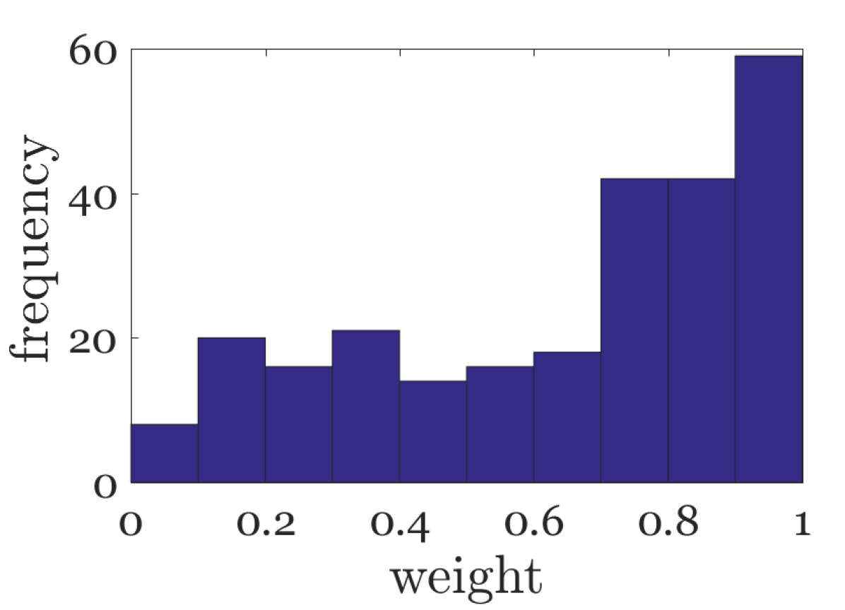
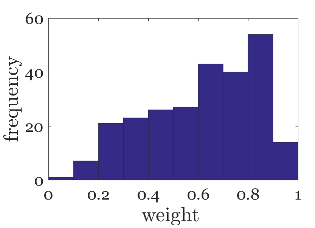
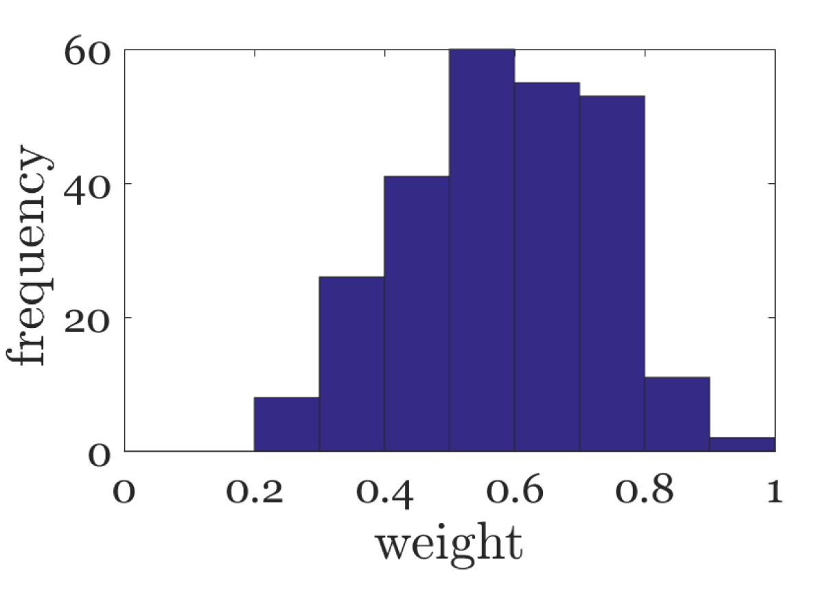
On the other hand, since the rain density is closely related to the weights , we could estimate the rain density from . As shown in Fig. 4(d), we illustrate the distribution of learned weights in Eq. (8), one can see that the weight cluster gradually approaches 1 with the increase of rain intensity. Therefore, we define the average of different channels as rain density estimation (RDE):
| (10) |
the more it rains, the greater RDE should be, as shown in Fig. 4(e). And RDEs of real raining images could be found in Section V-B. Note that all RDEs are normalized between zero and one.
Note that the weight is updated adaptively according to Eq. (9). It implies that the rain density is estimated without any labels in our model, instead of training an extra network in a supervised way to classify the rain density into three categories in DID-MDN [8]. Besides, thanks to the weights, our model is capable of estimating the rain density with continuous states, which is more suitable for real raining scenes than algorithms only classifying rain density into limited discrete states, for instance, DID-MDN [8].


(25.34, 0.8402)
(30.51, 0.9147)
(32.37, 0.9206)

(29.31, 0.8537)
(28.49, 0.8663)
(30.15, 0.8902)
(32.25, 0.9216)
(32.51, 0.9317)

(27.55, 0.7977)

(32.10, 0.9199)
(36.83, 0.9556)

(28.43, 0.8876)

(29.96, 0.8748)

(28.90, 0.8454)
(37.28, 0.9678)

( 37.67, 0.9670)
(20.59, 0.6078)

(29.89, 0.8860)

(23.31, 0.7231)

(29.12, 0.9144)
(21.95, 0.6959)

(33.11, 0.9289)

(33.21, 0.9328)

( 34.29, 0.9443)
(22.12, 0.6319)
(31.21, 0.8465)
(24.95, 0.7653)
(18.25, 0.7647)
(23.31, 0.7298)
(30.89, 0.8532)
(33.19, 0.8813)
(33.59, 0.8918)
0.4833

0.2433

0.3267

0.2467
0.1417
0.1333
0.1217
0.0667
0.5367
0.1967
0.1867
0.1733
0.3933
0.1883

0.1050

0.0900

0.0183

0.0067

0.0250

0.0083

0.0066

0.0133

0.0150

0.0100
0.3216
0.1350
0.1600
0.3017
0.0800
0.1017
0.0717
0.0683
III-C Network Architecture
In this section, we will introduce the network structure of CODE-Net, mainly consisting of rain streaks extractor and rain streaks denoiser.
Rain Streaks Extractor. We use two convolutional layers , to extract noisy rain streaks from the rainy input :
| (11) |
as shown in Fig. 2, can be seen as consisting of rain streaks and noise.
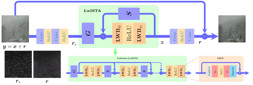
Rain Streaks Denoiser. is then fed into Eq. (8) to seek for the convolutional sparse code . To avoid long inference time, we build Eq. (8) by CNN techniques.
Specifically, for , under the assumption of nonnegative sparse coding, the soft nonnegative thresholding operator is equivalent to ReLU [21]. Thus, in Eq. (8), we replace with , where the threshold is learnable as well. Even though Eq. (12) is for one channel, the extension to multichannel case is mathematically straightforward. That is, for an input with channels, Eq. (12) still holds true with , , which means and correspond to two convolution layers. Above all, the resulting learning weighted ISTA (LwISTA) can be expressed as:
| (12) |
Based on Eq. (12), initializing to , the optimal convolutional sparse code could be produced efficiently after iterations. Note that shares the parameters over layers, as well as .
After obtaining the convolutional sparse code , to recover the noiseless rain streak , another dictionary corresponding to and a convolutional layer are needed:
| (13) |
Finally, the clean background image would be produced by subtracting rain streaks from the rainy image :
| (14) |
The whole architecture is illustrated in Fig. 2.
IV Multiscale CODE-Net: mCODE-Net
In deraining task, it is well studied in [22] that multiscale CSC performs better than traditional CSC since the rain streaks, captured from different distances, always appear to be multiscale. Inspired by this, we further extend CODE-Net to its multiscale version (mCODE-Net) to mine the potential, by expanding Eq. (2) to the following (three scales):
| (15) |
where and are rain filters of and representations corresponding to the -th dictionary.
Analogy to the solution procedure in Section III-A, one can obtain the convolutional sparse codes for the -th dictionary by:
| (16) |
and recover the noiseless rain streak by:
| (17) |
where can be implemented by several convolutional layers of . / and are learning weight blocks and threshold w.r.t. the -th dictionary.
V Experimental Results
V-A Settings
Datasets and Metrics. We use 12000 and 1800 pairs of images from [8, 6] and a high quality real rain dataset [7] as the training set. For testing, three commonly synthetic datasets, Rain1200 [8], Rain12 [2] and Test1000 [7], and some real-world images are utilized. The Rain1200 testing set, consisting of heavy, medium and light rain (Fig. 4(d)), is more challenging. Deraining results on synthetic datasets are evaluated with Peak Signal-to-Noise Ratio (PSNR) and Structural Similarity (SSIM) [23] on the Y channel of transformed YCbCr space, while the performance of real-world images is evaluated visually since the ground truth images are not available.
Model. In CODE-Net, each convolutional layer has filters () of size () except , and respectively having , () and filters. By contrast, we set , , and , , (namely, the rain filters are of size , and ) in mCODE-Net111Note that, even though mCODE-Net is multiscale, it has fewer parameters ( vs. ) than CODE-Net since fewer filters are exploited.. We desert the biases and use zero-padding to keep the size of feature maps fixed. Another important point is, differ from [5, 8], there is no BatchNormalization [24] in our models according to Eq. (12) and Eq. (16).
Training. To make full use of the limited images, we augment the training set with random horizontal flips and degree rotations. The training process is divided into two stages: (1) we train two plain models (CODE-Net/mCODE-Net without weighting), initialized by the method of He et al. [25], using loss in RGB channels. For optimization, we use Adam [26] with , . In each training batch, 8 patches of size are extracted as inputs. The learning rate is set to and halved at , , , iterations; (2) we then initialize CODE-Net and mCODE-Net using the plain models and fine-tune them with the learning rate set to and halved at , , , iterations. We use PyTorch to implement our models with an NVIDIA RTX 2080 GPU222Codes and more results are available at https://github.com/Achhhe/CODE-Net.
V-B Density Estimation of Synthetic and Real Rain
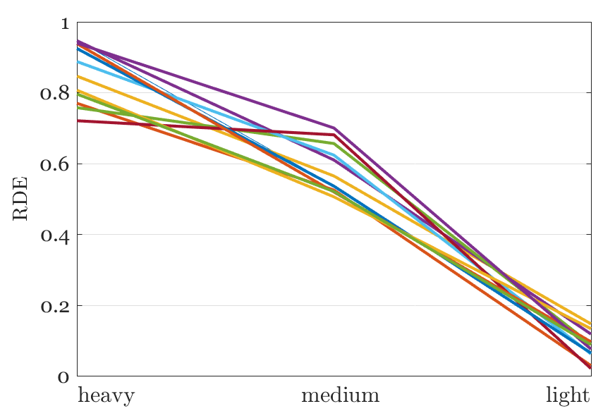
In this subsection, we focus on the rain density estimation of rainy images with synthetic and real rain. For synthetic rainy images, we show a sample of different rain levels in Fig. 4(d). And in Fig. 4(e), RDEs of several samples are depicted. One can see that, the RDEs mainly range from to and become larger as the rain density increases, consistent with the analysis in Section III-B.
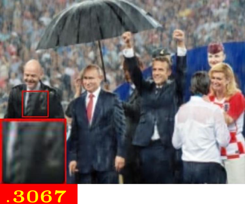
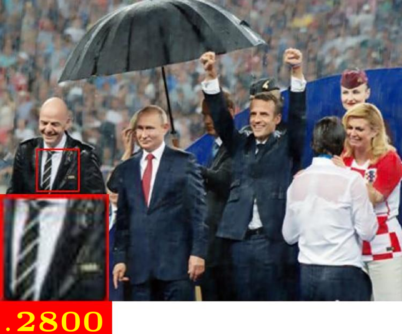
Besides, a clear image and some real-world rainy images with continuous rainy states and their RDEs are shown in Fig. 5. The clear image has the smallest RDE while the rainy images have gradual increased RDEs from to , which verifies the validity of continuous rain density estimation of our model.
| Methods | Rain12 | Rain1200 | Test1000 |
| PSNR/SSIM | PSNR/SSIM | PSNR/SSIM | |
| DSC*[1] | 29.98/0.8654 | 21.44/0.7896 | 32.33/0.9305 |
| GMM*[2] | 32.15/0.9145 | 22.75/0.8352 | 32.99/0.9475 |
| CNN [4] | 33.33/0.9199 | 23.55/0.8352 | 31.31/0.9304 |
| JORDER [6] | 36.15/0.9548 | 25.71/0.8074 | 35.72/0.9776 |
| DDN [5] | 29.84/0.9049 | 30.08/0.8791 | 34.88/0.9727 |
| DID-MDN [8] | 29.49 /0.9031 | 29.65/0.9016 | 28.96/0.9457 |
| PreNet [19] | 36.66 /0.9610 | 30.56/0.8750 | 30.31/0.9538 |
| SPANet [7] | 32.71 /0.9285 | 30.05/0.9342 | 38.53/ 0.9875 |
| CODE-Net (ours) | 36.21/ 0.9618 | 33.31 /0.9174 | 38.88/0.9867 |
| mCODE-Net (ours) | 36.79/ 0.9639 | 34.03/ 0.9281 | 39.85/0.9879 |
V-C Deraining Result Comparison
In this subsection, we compare our proposed CODE-Net and mCODE-Net to 9 state-of-the-art deraining methods, including DSC [1], GMM [2], CNN [4], DDN [5], JORDER [6], DID-MDN [8], SEMI [18], SPANet [7] and PreNet [19]. All results are reproduced by the authors’ codes except the quantitative ones of DSC and GMM on Rain1200 are cited from [8] directly since their codes run slowly.
Synthetic Images. Quantitative results are tabulated in Tab. I. Clearly, both CODE-Net and mCODE-Net achieve superior performance. Especially on Rain1200, the more complex dataset consisting of light, medium and heavy levels, our models outperform others by large margins, which indicates our models are more robust for different densities of rain. One important reason is that the rain density is implicitly considered in Eq. (8) and thus leads to better rain removal results. Fig. 6 and Fig. 7 show the visual comparisons. Our models consistently achieve the best visual performance in terms of effectively removing rain streaks while preserving background details. Besides, thanks to the multiscale prior, mCODE-Net could achieve comparable or even better results than CODE-Net with fewer parameters.
Note that, JORDER and DID-MDN use additional rain mask or density information in training stage. Nonetheless, our models still greatly outperform their results without any additional data.
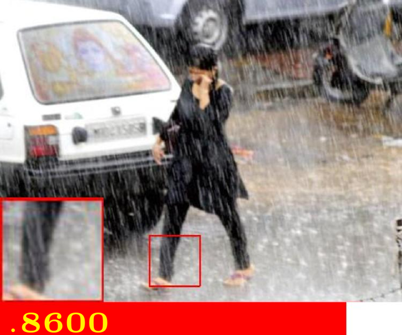
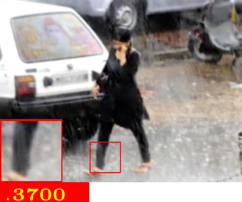
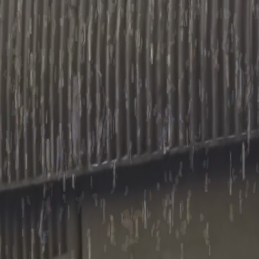
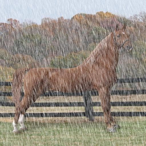
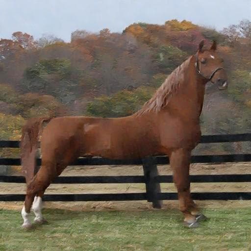
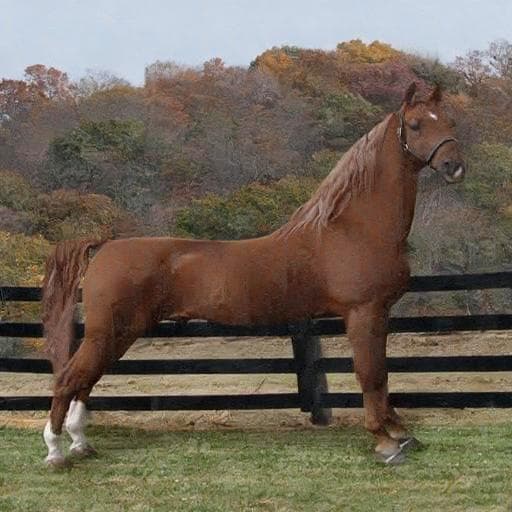
Real Images. To demonstrate the generalization of the proposed architectures, we evaluate our models and other methods on four real-world images, shown in Fig. 8 and Fig. 9. Once again, our models show the best visual performance. In contrast, previous methods especially DID-MDN tend to produce under/over deraining results. Our models get rid of these faults and produce more pleasant results, which verifies the effectiveness of continuous rain density estimation over classifying it into three levels.
Comparing CODE-Net and mCODE-Net, raindrops with large or small size can be efficiently removed by mCODE-Net with further consideration of the multi-scale property, while CODE-Net gives a result by leveraging different raindrop scales, as shown in Fig. 8.
We further apply the CODE-Net on the deraining results obtained by each method and use RDE Eq. (10) to estimate their rain densities. As shown in Fig. 8 and Fig. 9, the RDEs of the deraining images decrease comparing to the original rainy inputs, which reflects the deraining effects of each method. One can find that the proposed CODE-Net and mCODE-Net can achieve much lower RDEs than other methods for rainy images with heavy rains shown in Fig. 8. It coincides with the results on the synthetic rainy images as shown in Tab. I, where CODE-Net and mCODE-Net can outperform the state-of-the-arts by large margins.
On the other hand, the RDEs obtained from CODE-Net have potentials to quantitatively evaluate the deraining performance for rainy images from real scenes.
V-D Running Time Comparison
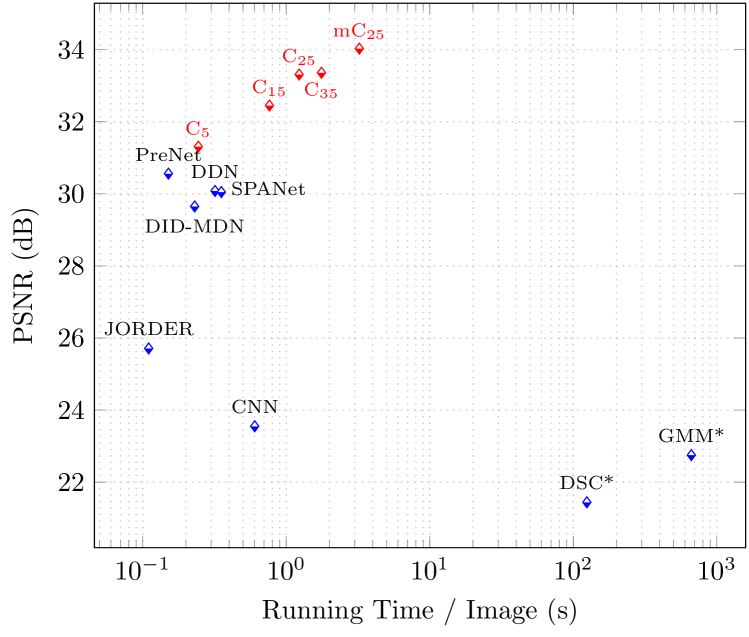
We visualize the running time per image () versus performance (PSNR) on Rain1200 dataset in Fig. 10. According to the provided source code, all methods are tested on GPU except DSC and GMM on CPU. One key factor affecting running time of our method is the number of iterations when solving convolutional sparse codes in Eq. (12). For simplicity, we denote CODE-Net/mCODE-Net iterating times as CT/mCT. It is observed that C5 achieves comparable performance and computational complexity as other state-of-the-art methods. However, too few iterations are not capable to generate good convolutional sparse codes. Hence, we additionally test three models with and unsurprisingly the results of them outperform those of other methods largely.
As shown in Fig. 10, with the increase of the number of iterations, the performance of our method can be further improved and obtain the optimal result when . In this paper, we focus on the best rain removal performance and thus choose in our final models (C25/mC25). For practical applications, we could adjust the number of iterations to balance performance and running time.
V-E Ablation Study
Our network (Fig. 2) is derived from traditional CSC problem, but by coincidence, it includes two common strategies in deep learning, i.e., local residual learning (LRL) [27] and pre-activation (PA) [28]. LRL is actually the local skip connection and PA means activation layer (LWB-ReLU-LWB) comes before weight layer () in unfolded LwISTA. Besides, to improve the deraining performance, we introduce reweighting (RW) into CSC optimization. Last but not the least, since their specific characteristics, we focus on extracting rain streaks and recover the deraining image by subtracting them from the input. Interestingly, this corresponds to the global residual learning (GRL).
(PSNR, SSIM)
(16.67, 0.5138)
(29.85, 0.8112)
(29.10, 0.8083)
To demonstrate the effectiveness of aforementioned components, we conduct an ablation study of GRL, LRL, PA and RW on CODE-Net. images are selected from Rain1200 for testing, with each level images. Tab. II shows the average PSNR. When both LRL and PA are used, the PSNR is relatively high, no matter RW is used or not (\nth2/\nth3 vs. \nth8/\nth9). Comparing \nth2/\nth4/\nth6/\nth8 with \nth3/\nth5/\nth7/\nth9, one can see that the performance could be improved by adding RW. However, it is interesting that, using PA only would degrade the performance (\nth2/\nth3 vs. \nth4/\nth5). Not surprisingly, CODE-Net using four components simultaneously performs the best. These comparisons indicate the superiority of reweighted CSC inspired network combining GRL, LRL, PA and RW in a particular way.
| GRL | LRL | PA | RW | PSNR | ||||
| \nth1 | ✘ | ✔ | ✔ | ✔ | 30.56 | |||
| \nth2 | ✔ | ✘ | ✘ | ✘ | 29.40 | |||
| \nth3 | ✔ | ✘ | ✘ | ✔ | 30.00 | |||
| \nth4 | ✔ | ✘ | ✔ | ✘ | 29.34 | |||
| \nth5 | ✔ | ✘ | ✔ | ✔ | 29.92 | |||
| \nth6 | ✔ | ✔ | ✘ | ✘ | 29.85 | |||
| \nth7 | ✔ | ✔ | ✘ | ✔ | 30.88 | |||
| \nth8 | ✔ | ✔ | ✔ | ✘ | 29.58 | |||
| \nth9 | ✔ | ✔ | ✔ | ✔ | 31.05 |
V-F Failure Cases
Though the proposed network could achieve superior performance on most of testing images while producing corresponding RDEs, some situations occurred in which our method would produce overestimation of RDE and over deraining result, as exhibited in Fig. 11. This is primarily caused by the confusing of rain-like structures and the crude global average pooling operation in LWB Eq. (9) that only considers the overall information of each channle. We believe that the predicament could be tackled if we capture sufficient local details additionally.
V-G Extensions
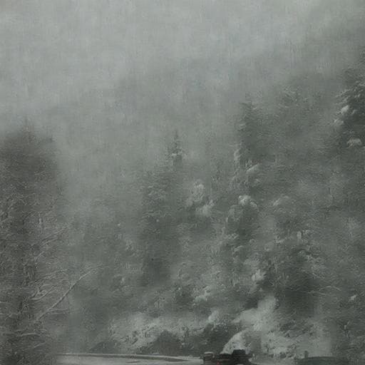
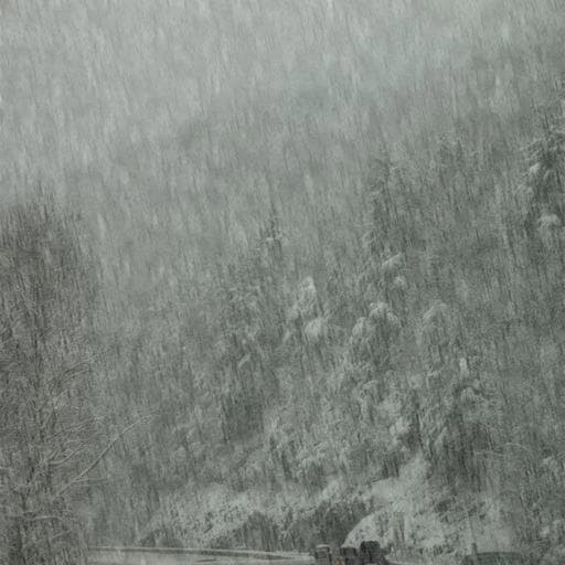
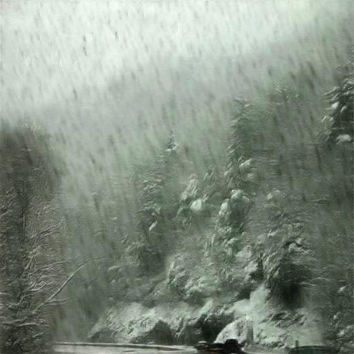
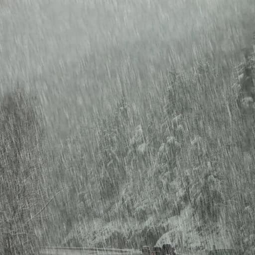
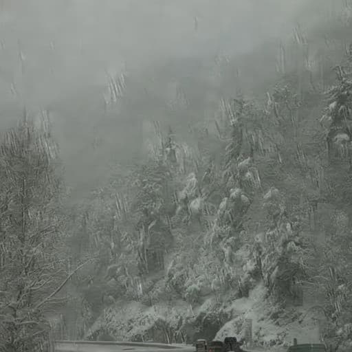
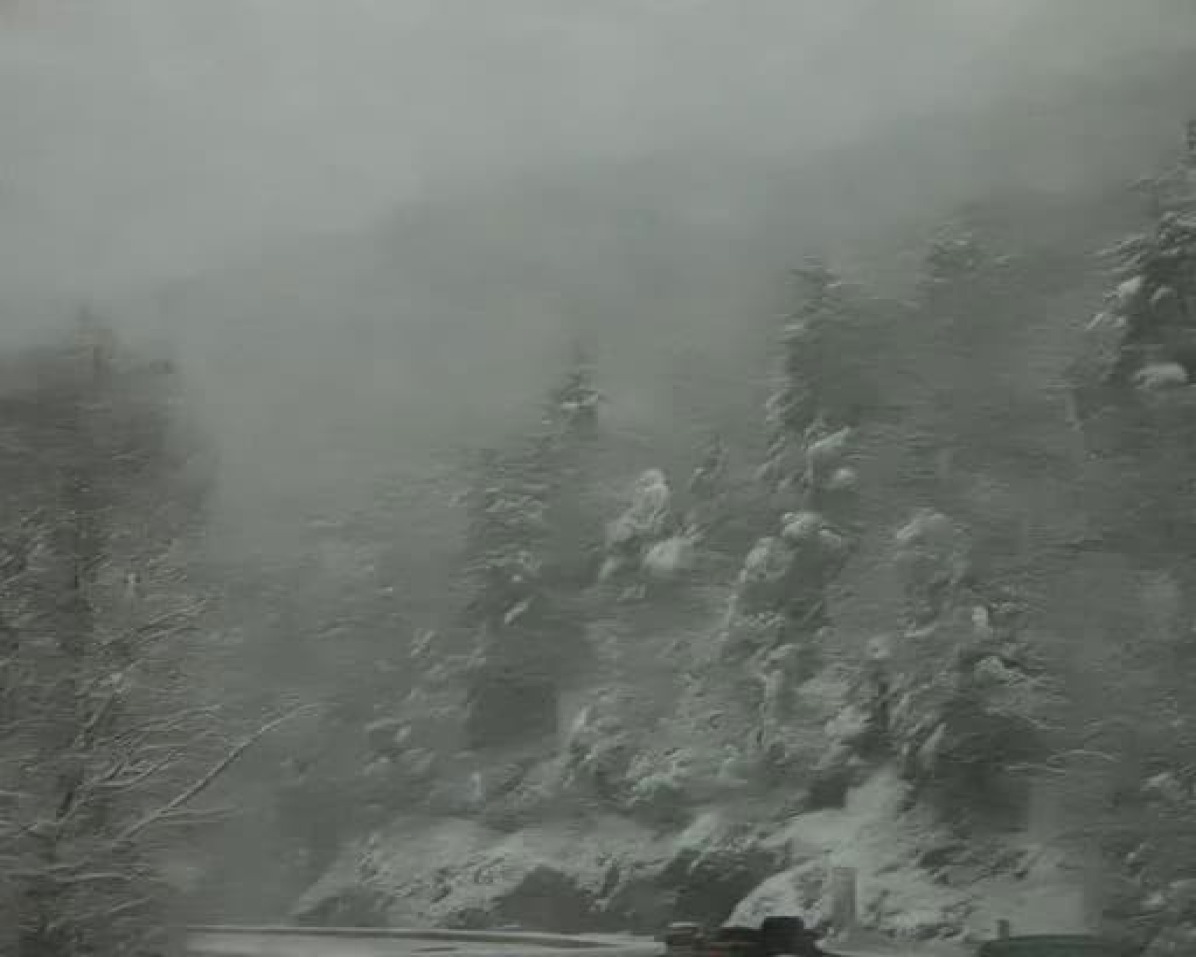
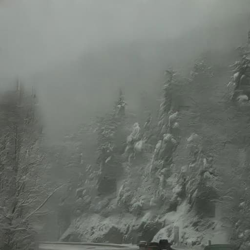
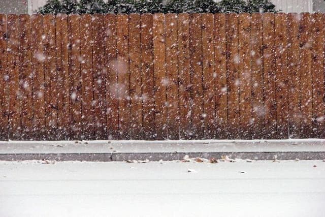
In this section, we explore the potentials of our network for other visual tasks. In the pursuit of better deraining effect, we first train a generative adversarial CODE-Net (GaCODE-Net) using perceptual loss [29, 30]. As shown in Fig. 13(e), although inferior to CODE-Net on quantitative metrics (PSNR and SSIM), GaCODE-Net is capable of generating more realistic textures and high-frequency details. Moreover, since snowy image could be modeled as Eq. (1) [31] and snow streaks share much similarity with rain streaks, we then evaluate our CODE-Net on image desnowing task. Fig. 13(h) shows the results on two real snowy images, which verifies the promising generalization of our method on other tasks with similar degeneration model.
VI Conclusion
Single image deraining with unknown rain densities and multi-scale raindrops are very challenging and rarely considered in literatures. In this paper, a density guided network (CODE-Net) and its multi-scale version mCODE-Net are proposed, where both rain density and raindrop scale are considered. Representing rain streaks with the CSC model, we find that the sparse coefficients of rain streaks and the rain density are closely related. Consequently, the rain density is implicitly considered by learning weights from sparse coefficients through the channel attention blocks. And extending CODE-Net to multi-scale dictionaries, the challenge of multi-scale raindrops for SIDR can be straightforwardly addressed. Both qualitative and quantitative evaluations demonstrate the superiority to recent state-of-the-art methods. Extensions to applications of other low-level vision tasks are also explored and show the generality of our proposed CODE-Net.
Moreover, with the learned weights, we proposed a simple approach, namely RDE, to estimate the continuously valued rain density. The effectiveness of RDE is validated in various clean, rainy and derained images, while the potential for evaluating deraining algorithms is reserved for future works. Besides, to obtain more precise weights, we plan to improve the learning weight block , such as leveraging more local details, e.g., spatial structure and nonlocal self-similarity.
References
- [1] Y. Luo, Y. Xu, and H. Ji, “Removing rain from a single image via discriminative sparse coding,” in ICCV, 2015, pp. 3397–3405.
- [2] Y. Li, R. T. Tan, X. Guo, J. Lu, and M. S. Brown, “Rain streak removal using layer priors,” in CVPR, 2016, pp. 2736–2744.
- [3] X. Lin, L. Ma, B. Sheng, Z. Wang, and W. Chen, “Utilizing two-phase processing with fbls for single image deraining,” IEEE Transactions on Multimedia, pp. 1–1, 2020.
- [4] X. Fu, J. Huang, X. Ding, Y. Liao, and J. Paisley, “Clearing the skies: A deep network architecture for single-image rain removal,” IEEE TIP, vol. 26, no. 6, pp. 2944–2956, 2017.
- [5] X. Fu, J. Huang, D. Zeng, Y. Huang, X. Ding, and J. Paisley, “Removing rain from single images via a deep detail network,” in CVPR, 2017, pp. 3855–3863.
- [6] W. Yang, R. T. Tan, J. Feng, J. Liu, Z. Guo, and S. Yan, “Deep joint rain detection and removal from a single image,” in CVPR, 2017, pp. 1357–1366.
- [7] T. Wang, X. Yang, K. Xu, S. Chen, Q. Zhang, and R. W. Lau, “Spatial attentive single-image deraining with a high quality real rain dataset,” in CVPR, 2019, pp. 12 270–12 279.
- [8] H. Zhang and V. M. Patel, “Density-aware single image de-raining using a multi-stream dense network,” in CVPR, 2018, pp. 695–704.
- [9] M. D. Zeiler, D. Krishnan, G. W. Taylor, and R. Fergus, “Deconvolutional networks,” in CVPR, 2010, pp. 2528–2535.
- [10] Y. Zhang, K. Li, K. Li, L. Wang, B. Zhong, and Y. Fu, “Image super-resolution using very deep residual channel attention networks,” in ECCV, 2018.
- [11] J. Hu, L. Shen, and G. Sun, “Squeeze-and-excitation networks,” in CVPR, 2018, pp. 7132–7141.
- [12] E. J. Candes, M. B. Wakin, and S. P. Boyd, “Enhancing sparsity by reweighted minimization,” Journal of Fourier analysis and applications, vol. 14, no. 5-6, pp. 877–905, 2008.
- [13] D. L. Donoho, “Compressed sensing,” IEEE Transactions on Information Theory, vol. 52, no. 4, pp. 1289–1306, 2006.
- [14] L.-W. Kang, C.-W. Lin, and Y.-H. Fu, “Automatic single-image-based rain streaks removal via image decomposition,” IEEE TIP, vol. 21, no. 4, pp. 1742–1755, 2011.
- [15] L. Zhu, C.-W. Fu, D. Lischinski, and P.-A. Heng, “Joint bi-layer optimization for single-image rain streak removal,” in ICCV, 2017, pp. 2526–2534.
- [16] Y.-L. Chen and C.-T. Hsu, “A generalized low-rank appearance model for spatio-temporally correlated rain streaks,” in ICCV, 2013, pp. 1968–1975.
- [17] J.-H. Kim, C. Lee, J.-Y. Sim, and C.-S. Kim, “Single-image deraining using an adaptive nonlocal means filter,” in ICIP. IEEE, 2013, pp. 914–917.
- [18] W. Wei, D. Meng, Q. Zhao, Z. Xu, and Y. Wu, “Semi-supervised transfer learning for image rain removal,” in CVPR, 2019.
- [19] D. Ren, W. Zuo, Q. Hu, P. Zhu, and D. Meng, “Progressive image deraining networks: A better and simpler baseline,” in CVPR, 2019.
- [20] X. Li, J. Wu, Z. Lin, H. Liu, and H. Zha, “Recurrent squeeze-and-excitation context aggregation net for single image deraining,” in ECCV, 2018, pp. 262–277.
- [21] V. Papyan, Y. Romano, and M. Elad, “Convolutional neural networks analyzed via convolutional sparse coding,” Journal of Machine Learning Research, vol. 18, no. 1, pp. 2887–2938, 2017.
- [22] M. Li, Q. Xie, Q. Zhao, W. Wei, S. Gu, J. Tao, and D. Meng, “Video rain streak removal by multiscale convolutional sparse coding,” in CVPR, 2018, pp. 6644–6653.
- [23] Z. Wang, A. C. Bovik, H. R. Sheikh, E. P. Simoncelli et al., “Image quality assessment: from error visibility to structural similarity,” IEEE TIP, vol. 13, no. 4, pp. 600–612, 2004.
- [24] S. Ioffe and C. Szegedy, “Batch normalization: Accelerating deep network training by reducing internal covariate shift,” in ICML, 2015, pp. 448–456.
- [25] K. He, X. Zhang, S. Ren, and J. Sun, “Delving deep into rectifiers: Surpassing human-level performance on imagenet classification,” ICCV, pp. 1026–1034, 2015.
- [26] D. P. Kingma and J. Ba, “Adam: A method for stochastic optimization,” arXiv preprint arXiv:1412.6980, 2014.
- [27] Y. Tai, J. Yang, and X. Liu, “Image super-resolution via deep recursive residual network,” in CVPR, 2017, pp. 3147–3155.
- [28] K. He, X. Zhang, S. Ren, and J. Sun, “Identity mappings in deep residual networks,” in ECCV. Springer, 2016, pp. 630–645.
- [29] C. Ledig, L. Theis, F. Huszár, J. Caballero, A. Cunningham, A. Acosta, A. Aitken, A. Tejani, J. Totz, Z. Wang et al., “Photo-realistic single image super-resolution using a generative adversarial network,” in CVPR, 2017, pp. 4681–4690.
- [30] J. Johnson, A. Alahi, and L. Fei-Fei, “Perceptual losses for real-time style transfer and super-resolution,” in ECCV. Springer, 2016, pp. 694–711.
- [31] J. Tian, Z. Han, W. Ren, X. Chen, and Y. Tang, “Snowflake removal for videos via global and local low-rank decomposition,” IEEE Transactions on Multimedia, vol. 20, no. 10, pp. 2659–2669, 2018.