¹¹institutetext: Department of Information Engineering, Hiroshima University, 1-4-1 Kagamiyama, Higashi-Hiroshima, 739-8527 Japan ²²institutetext: Graduate School of Advanced Science and Engineering, Hiroshima University, 1-4-1 Kagamiyama, Higashi-Hiroshima-shi, Hiroshima739-8527, Japan ²²email: {m191504,lukman-hakim,tkurita, miyao}@hiroshima-u.ac.jp

Single-Image Super-Resolution Reconstruction based on the Differences of Neighboring Pixels^†^†thanks: Supported by organization x.

Huipeng Zheng 11 Lukman Hakim 11 Takio Kurita 22 Junichi Miyao 22

Abstract

The deep learning technique was used to increase the performance of single image super-resolution (SISR). However, most existing CNN-based SISR approaches primarily focus on establishing deeper or larger networks to extract more significant high-level features. Usually, the pixel-level loss between the target high-resolution image and the estimated image is used, but the neighbor relations between pixels in the image are seldom used. On the other hand, according to observations, a pixel’s neighbor relationship contains rich information about the spatial structure, local context, and structural knowledge. Based on this fact, in this paper, we utilize pixel’s neighbor relationships in a different perspective, and we propose the differences of neighboring pixels to regularize the CNN by constructing a graph from the estimated image and the ground-truth image. The proposed method outperforms the state-of-the-art methods in terms of quantitative and qualitative evaluation of the benchmark datasets.

Keywords:

Super-resolution Convolutional Neural Networks Deep Learning.

1 Introduction

Single-Image Super-Resolution (SISR) is a technique to reconstruct a high-resolution (HR) image from a low-resolution (LR) image. The challenges problem in the super-resolution task is the ill-pose problem. Many SISR techniques have been developed to address this challenge, including interpolation-based[1, 2], reconstruction-based[3], and deep learning-based methods[4].

Even though CNN-based SISR has significantly improved learning-based approaches bringing good performances, existing SR models based on CNN still have several drawbacks. Most SISR techniques based on CNN are primarily concerned with constructing deeper or larger networks to acquire more meaningful high-level features. Usually, we use the pixel-level loss between the target high-resolution image and the estimated image and neglect the neighbor relations between pixels.

Basically, natural images have a strong pixel neighbor relationship. It means that a pixel has a strong correlation with its neighbors, but a low correlation with or is largely independent of pixels further away[11]. In addition, the neighboring relationship of a pixel also contains rich information about the spatial structure, local context, and structural knowledge[7]. Based on this fact, the authors proposed to introduce the pixel neighbor relationships as a regularizer in the loss function of CNN and applied for Anime-like Images Super-Resolution and Fundus Image Segmentation[5]. The regularizer is named Graph Laplacian Regularization based on the Differences of Neighboring Pixels (GLRDN). The GLRDN is essentially deriving from the graph theory approach. The graph is constructed from the estimated image and the ground-truth image. The graphs use the pixel as a node and the edge represented by the ”differences” of a neighboring pixel. The basic idea is that the differences between the neighboring pixels in the estimated images should be close to the differences in the ground-truth image.

This study propose the GLRDN for general single image super-resolution and show the effectiveness of the proposed approach by introducing the GLRDN to the state-of-the-art SISR methods (EDSR[6] and RCAN[12]). The proposed GLRDN can combine with the existing CNN-based SISR methods as a regularizer by simply adding the GLRDN term into their loss functions. We can easily improve the quality of the estimated super-resolution image of the existing SISR methods.

The contribution of this paper can summarize as follow : (1) Proposed GLRDN to capture the relationship between neighboring pixels for general single image super-resolution; (2) Analyzed the baseline architecture with and without our regularizer; (3) Explored our proposed methods with state-of-the-art methods in single image super-resolution.

The structure of this paper is as follows. In Section 2, we presented some related methods with our work. In section 3, we explain the proposed method. The results and experiments are detailed in Section 4. Finally, section 5 is presented the conclusion of this study.

2 Related Work

2.1 Graph Laplacian Regularization based on the Differences of Neighboring Pixels

The GLRDN was proposed by Hakim et al.[5]. This regularizer uses the graph theory approach to capture the relationship of the difference between pixels. Assume that we have two images, estimated image $y$ and target image $t$ . Then $G=(V,E)$ constructed be a graph where $V=\{i|i=1,\ldots,N\}$ is the set of the pixel indices with $N$ pixels and the $E=\{(i,j)|i,j\in V\}$ is the neighboring relations between the pixels. Furthermore, the differences of neighboring pixels of two images $s_{G}$ are given as

$\displaystyle S_{G}(\bm{t},\bm{y})$	$\displaystyle=\sum_{(i,j)\in E}\{(t_{i}-t_{j})-(y_{i}-y_{j})\}^{2}$
	$\displaystyle=\sum_{(i,j)\in E}(\Delta t_{ij}-\Delta y_{ij})^{2}$
	$\displaystyle=(\Delta\bm{t}-\Delta\bm{y})^{T}(\Delta\bm{t}-\Delta\bm{y})$
	$\displaystyle=(B\bm{t}-B\bm{y})^{T}(B\bm{t}-B\bm{y})$
	$\displaystyle=(\bm{t}-\bm{y})^{T}B^{T}B(\bm{t}-\bm{y})$
	$\displaystyle=(\bm{t}-\bm{y})^{T}L(\bm{t}-\bm{y})$	(1)

where $B$ is incident matrix and $L$ is the Laplacian matrix that is defined from the identity matrix.

3 Method

This study aims to capture neighboring pixel’s relationships from the reconstructed image estimated from the LR image and the HR images and minimize the differences of the adjacent pixels differences. As a result, the loss is defined as the squared errors of the differencess between the predicted image and HR images. In the following sections, we will go through the specifics of the proposed approach.

3.1 Estimation of the Differences Neighboring Pixels

Let us consider the set of training samples $X=\{(\bm{x}_{m},\bm{t}_{m})|m=1,...,M\}$ where $\bm{x}_{m}$ is a $m^{th}$ input image and $\bm{t}_{m}$ is the $m^{th}$ target image. $M$ is define as the total of images in training samples. The network is trained to predict the output HR image $\bm{y}_{m}$ from the $m^{th}$ input LR image $\bm{x}_{m}$ .

The GLRDN is defined as the graph, which is pixels as nodes and sum of the squared differences of the differences of neighboring pixels between the target image $\bm{t}_{m}$ and the estimated images $\bm{y}_{m}$ as edges. Then the GLRDN is given as

\displaystyle S_{G}

\displaystyle=\sum_{m=1}^{M}S_{G}(\bm{t}_{m},\bm{y}_{m})=\sum^{M}_{m=1}(\bm{t}_{m}-\bm{y}_{m})^{T}L(\bm{t}_{m}-\bm{y}_{m})

(2)

This measure $S_{G}$ becomes small if the neighboring relations of the pixels in the estimated output images are similar to those of the target images.

3.2 CNN-based Super-Resolution with GLRDN

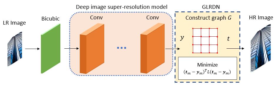
We can apply the proposed GLRDN to any existing CNN-based Super-Resolution algorithms by simply adding the GLRDN term in the loss function for the training. The proposed method is illustrated in Fig. 1. The CNN-based Super-Resolution is trained to estimate the HR image as $y$ for a given LR input image $x$ . The first convolutional layer retrieves a series of feature maps. The second layer non-linearly transfers these feature maps to high-resolution patch representations. To construct the final high-resolution image, the last layer integrates the estimates within a spatial neighborhood.

Refer to caption — Figure 1: Illustration of the proposed method on CNN-based Super-Resolution

In the Super-resolution task, using the Sum Squared Error (SSE) as the objective function is common. The Sum Squared Error is given by

E_{sse}=\sum^{M}_{m=1}(\bm{t}_{m}-\bm{y}_{m})^{2}

(3)

For the training of the parameters of the network, we combine the SSE loss with the regularization term as

Q_{sr}=E_{sse}+\lambda S_{G}

(4)

where $\lambda$ is a parameter to adjust the regularization. The network learning process is more robust by adding the term regularization because it considers the relationship between pixels rather than just comparing pixels with pixels.

4 Experiments

4.1 Experimental Setting

We adopt the EDSR and RCAN as our baseline models due to their great performance on image super-resolution tasks. In all these settings, we compare the performance with and without our regularizer. We set 300 epochs and batch size to 16. We set the learning rate to $10^{-4}$ and divided at every $2\times 10^{5}$ minibatch.

Our experiments are performed under the $\times 2$ , $\times 3$ , $\times 4$ scale factor. During training, we use the RGB input patches with the size of $48\times 48$ in each batch. Augmentation technique also used on the training images by rotating $90^{\circ}$ , $180^{\circ}$ , $270^{\circ}$ , and flipped randomly. This experiments implemented on DIV2K[13], Set5[14], Set14[15], B100[10], Urban100[9], and Manga109[8] datasets. We asses the improvement of our method using PSNR and SSIM measurements.

Table 1: Ablation study on Set5, Set14, and B100 datasets.

Method	$\lambda$	Set5		Set14		B100
Method	$\lambda$	PSNR	SSIM	PSNR	SSIM	PSNR	SSIM
Bicubic	-	28.42	0.8104	26.00	0.7027	25.96	0.6675
EDSR	0	30.89	0.8683	27.66	0.7515	27.12	0.7159
EDSR+ours	0.1	31.69	0.8851	28.15	0.7655	27.49	0.7279
EDSR+ours	1	31.75	0.8863	28.19	0.7663	27.52	0.7643
EDSR+ours	5	31.74	0.8857	28.18	0.7653	27.52	0.7262
EDSR+ours	10	31.75	0.8855	28.18	0.7641	27.52	0.7252
EDSR+ours	100	31.65	0.8840	28.12	0.7620	27.49	0.7230

Table 2: Ablation study on Urban100 and Manga109 datasets.

Method	$\lambda$	Urban100		Manga109
Method	$\lambda$	PSNR	SSIM	PSNR	SSIM
Bicubic	-	23.14	0.6577	24.89	0.7866
EDSR	0	25.12	0.7445	29.68	0.8999
EDSR+ours	0.1	25.83	0.7749	30.84	0.9061
EDSR+ours	1	25.92	0.7749	30.95	0.9084
EDSR+ours	5	25.95	0.7767	30.91	0.9072
EDSR+ours	10	25.95	0.7762	30.86	0.9062
EDSR+ours	100	25.92	0.7736	30.84	0.9042

5 Result and Discussion

Table 3: Performance of our proposed method compared with the state of the art method.

Method	scale	Set5		Set14		B100		Urban100		Manga109
Method	scale	PSNR	SSIM	PSNR	SSIM	PSNR	SSIM	PSNR	SSIM	PSNR	SSIM

Bicubic	x2	33.66	0.9299	30.24	0.8688	29.56	0.8431	26.88	0.8403	30.80	0.9339
SRCNN	x2	36.66	0.9542	32.45	0.9067	31.36	0.8879	29.50	0.8946	35.60	0.9663
FSRCNN	x2	37.05	0.9560	32.66	0.9090	31.53	0.8920	29.88	0.9020	36.67	0.9710
VDSR	x2	37.53	0.9590	33.05	0.9130	31.90	0.8960	30.77	0.9140	37.22	0.9750
LapSRN	x2	37.52	0.9591	33.08	0.9130	31.08	0.8950	30.41	0.9101	37.27	0.9740
MemNet	x2	37.78	0.9597	33.28	0.9142	32.08	0.8978	31.31	0.9195	37.72	0.9740
EDSR	x2	38.07	0.9606	33.65	0.9167	32.20	0.9004	31.88	0.9214	38.22	0.9763
SRMDNF	x2	37.79	0.9601	33.32	0.9159	32.05	0.8985	31.33	0.9204	38.07	0.9761
D-DBPN	x2	38.09	0.9600	33.85	0.9190	32.27	0.9006	32.55	0.9324	38.89	0.9775
RDN	x2	38.24	0.9614	34.01	0.9212	32.34	0.9017	32.89	0.9353	39.18	0.9780
RCAN	x2	38.25	0.9608	34.08	0.9213	32.38	0.9020	33.29	0.9363	39.22	0.9778
EDSR+(ours)	x2	38.17	0.9610	33.74	0.9182	32.25	0.9000	31.96	0.9248	38.57	0.9764
RCAN+(ours)	x2	38.31	0.9612	34.20	0.9222	32.39	0.9022	33.30	0.9369	39.27	0.9781

Bicubic	x3	30.39	0.8682	27.55	0.7742	27.21	0.7385	24.46	0.7349	26.95	0.8556
SRCNN	x3	32.75	0.9090	29.30	0.8215	28.41	0.7863	26.24	0.7989	30.48	0.9117
FSRCNN	x3	33.18	0.9140	29.37	0.8240	28.53	0.7910	26.43	0.8080	31.10	0.9210
VDSR	x3	33.67	0.9210	29.78	0.8320	28.83	0.7990	27.14	0.8290	32.01	0.9340
LapSRN	x3	33.82	0.9227	29.87	0.8320	28.82	0.7980	27.07	0.8280	32.21	0.9350
MemNet	x3	34.09	0.9248	30.00	0.8350	28.96	0.8001	27.56	0.8376	32.51	0.9369
EDSR	x3	34.26	0.9252	30.08	0.8418	29.20	0.8106	28.48	0.8638	33.20	0.9415
SRMDNF	x3	34.12	0.9254	30.04	0.8382	28.97	0.8025	27.57	0.8398	33.00	0.9403
RDN	x3	34.71	0.9296	30.57	0.8468	29.26	0.8093	28.80	0.8653	34.13	0.9484
RCAN	x3	34.79	0.9255	30.39	0.8374	29.40	0.8158	29.24	0.8804	33.99	0.9469
EDSR+(ours)	x3	34.41	0.9253	30.18	0.8443	29.27	0.8141	28.49	0.8672	33.76	0.9416
RCAN+(ours)	x3	34.85	0.9259	30.50	0.8392	29.41	0.8186	29.25	0.8838	34.15	0.9484

Bicubic	x4	28.42	0.8104	26.00	0.7027	25.96	0.6675	23.14	0.6577	24.89	0.7866
SRCNN	x4	30.48	0.8628	27.50	0.7513	26.90	0.7101	24.52	0.7221	27.58	0.8555
FSRCNN	x4	30.72	0.8660	27.61	0.7550	26.98	0.7150	24.62	0.7280	27.90	0.8610
VDSR	x4	31.35	0.8830	28.02	0.7680	27.29	0.7260	25.18	0.7540	28.83	0.8870
LapSRN	x4	31.54	0.8850	28.19	0.7720	27.32	0.7270	25.21	0.7560	29.09	0.8900
MemNet	x4	31.74	0.8893	28.26	0.7723	27.40	0.7281	25.50	0.7630	29.42	0.8942
EDSR	x4	32.04	0.8926	28.43	0.7755	27.70	0.7351	26.45	0.7908	30.25	0.9028
SRMDNF	x4	31.96	0.8925	28.35	0.7787	27.49	0.7337	25.68	0.7731	30.09	0.9024
D-DBPN	x4	32.47	0.8980	28.82	0.7860	27.72	0.7400	26.38	0.7946	30.91	0.9137
RDN	x4	32.47	0.8990	28.81	0.7871	27.72	0.7419	26.61	0.8028	31.00	0.9151
RCAN	x4	32.78	0.8988	28.68	0.7832	27.85	0.7418	27.07	0.8121	31.02	0.9157
EDSR+(ours)	x4	32.21	0.8934	28.51	0.7768	27.75	0.7369	26.52	0.7937	30.53	0.9057
RCAN+(ours)	x4	32.90	0.8992	28.79	0.7849	27.86	0.7423	27.13	0.8139	31.10	0.9163

Ablation Study. In this part, the ablation study presented the effect of the proposed regularizer. We combined EDSR with our regularizer by setting different $\lambda$ . We started with a simple EDSR model by setting the number of layers $B$ = 12 and the number of feature channels $F$ = 64 with a scaling factor of 1. We compared the PSNR/SSIM result on the different testing datasets by setting the scale factor as 4. Table 1 showing the ablation study on Set5, Set14, and B100 datasets, and Table 2 showing the ablation study on Urban100 and Manga109 datasets. The best results are highlighted in bold. As shown in Table 1 and Table 2, the best parameter $\lambda$ in Eq. 4 is 1 which highest PSNR and SSIM on Set5, Set14, B100, and Manga109 datasets. Meanwhile, we found that $\lambda$ =5 is the best on Urban100 datasets. We obtained these values by performing parameter experiments in the ranges 0 to 100, $\lambda$ =0 means we use only EDSR as a baseline without a regularizer. Along with increasing lambda, the stronger the influence of the relationship between pixels in the learning process. Compared to baseline, our approach achieved an improvement of PSNR and SSIM scores over all datasets.

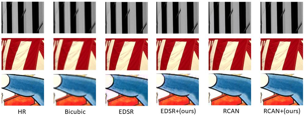
Comparation with state-of-the-art. To know the advantages of our proposed regularizer, we combine our regularizer with EDSR and RCAN and then compare the result with state-of-the-art CNN-based SR methods. Table 3 summarizes all of the quantitative data for the various scaling factors. The best results are highlighted in bold. Compared to competing approaches, joining RCAN and our methods achieve the best results across all datasets and scaling factors. The qualitative result of our approach is shown in Fig. 2. To know the differences in detail, we zoomed in on a portion of the image area. Fig. 2 showing our approach demonstrated more realistic visual results compared to other methods on Urban100, B100, and Manga109 datasets. It means the proposed regularizer succeeds in reconstructing the details of the HR image generate from the LR image compared over baseline methods.

6 Conclusion

This paper shows that the differences in pixels neighbor relationships can establish the network more robust on super-resolution tasks. Our method employs the adjacent pixels differences as a regularizer with existing CNN-based SISR methods to ensure that the differences between pixels in the estimated image are close to different pixels in the ground truth images. The experimental findings on five datasets demonstrate that our method outperforms the baseline CNN without regularization. Our proposed method generates more detailed visual results and improved PSNR/SSIM scores compared to other state-of-the-art methods. Future work will implement the differences in pixel neighbor relationships as a regularizer on different computer vision tasks.

Acknowledgments

This work was partly supported by JSPS KAKENHI Grant Number 21K12049.

References

[1] Zhou, F., Yang, W., and Liao, Q. (2012). Interpolation-based image super-resolution using multisurface fitting. IEEE Transactions on Image Processing, 21(7), 3312-3318.
[2] Anbarjafari, G., and Demirel, H. (2010). Image super resolution based on interpolation of wavelet domain high frequency subbands and the spatial domain input image. ETRI journal, 32(3), 390-394.
[3] K. Zhang, X. Gao, D. Tao, and X. Li. Single image superresolution with non-local means and steering kernel regression. TIP, 2012.
[4] Dong, C., Loy, C. C., He, K., and Tang, X. (2014, September). Learning a deep convolutional network for image super-resolution. In European conference on computer vision (pp. 184-199). Springer, Cham.
[5] Hakim, L., Zheng, H., Kurita, T. (2021). Improvement for Single Image Super-resolution and Image Segmentation by Graph Laplacian Regularizer based on Differences of Neighboring Pixels. Manuscript submitted for publication.
[6] Lim, B., Son, S., Kim, H., Nah, S., and Mu Lee, K. (2017). Enhanced deep residual networks for single image super-resolution. In Proceedings of the IEEE conference on computer vision and pattern recognition workshops (pp. 136-144).
[7] Zhou, W., Wang, Y., Chu, J., Yang, J., Bai, X., and Xu, Y. (2020). Affinity Space Adaptation for Semantic Segmentation Across Domains. IEEE Transactions on Image Processing.
[8] Matsui, Y., Ito, K., Aramaki, Y., Fujimoto, A., Ogawa, T., Yamasaki, T., and Aizawa, K. (2017). Sketch-based manga retrieval using manga109 dataset. Multimedia Tools and Applications, 76(20), 21811-21838.
[9] Huang, J. B., Singh, A., and Ahuja, N. (2015). Single image super-resolution from transformed self-exemplars. In Proceedings of the IEEE conference on computer vision and pattern recognition (pp. 5197-5206).
[10] Martin, D., Fowlkes, C., Tal, D., and Malik, J. (2001, July). A database of human segmented natural images and its application to evaluating segmentation algorithms and measuring ecological statistics. In Proceedings Eighth IEEE International Conference on Computer Vision. ICCV 2001 (Vol. 2, pp. 416-423). IEEE.
[11] Zhang, Z., Wang, X., and Jung, C. (2018). DCSR: Dilated convolutions for single image super-resolution. IEEE Transactions on Image Processing, 28(4), 1625-1635.
[12] Zhang, Y., Li, K., Li, K., Wang, L., Zhong, B., and Fu, Y. (2018). Image super-resolution using very deep residual channel attention networks. In Proceedings of the European conference on computer vision (ECCV) (pp. 286-301).
[13] Agustsson, E., and Timofte, R. (2017). Ntire 2017 challenge on single image super-resolution: Dataset and study. In Proceedings of the IEEE Conference on Computer Vision and Pattern Recognition Workshops (pp. 126-135).
[14] Bevilacqua, M., Roumy, A., Guillemot, C., and Alberi-Morel, M. L. (2012). Low-complexity single-image super-resolution based on nonnegative neighbor embedding.
[15] Zeyde, R., Elad, M., and Protter, M. (2010, June). On single image scale-up using sparse-representations. In International conference on curves and surfaces (pp. 711-730). Springer, Berlin, Heidelberg.

Single-Image Super-Resolution Reconstruction based on the Differences of Neighboring Pixels††thanks: Supported by organization x.