Single Pulse Manipulations in Synthetic Time-frequency Space
Abstract
Synthetic dimensions in photonic structures provide unique opportunities for actively manipulating light in multiple degrees of freedom. Here, we theoretically explore a dispersive waveguide under the dynamic phase modulation that supports single pulse manipulations in the synthetic (2+1) dimensions. Compared with the counterpart of the conventional (2+1) space-time, we explore temporal diffraction and frequency conversion in a synthetic time-frequency space while the pulse evolves along the spatial dimension. By introducing the effective gauge potential well for photons in the synthetic time-frequency space with the control of the modulation phase, we show that a rich set of pulse propagation behaviors can be achieved, including confined pulse propagation, fast/slow light, and pulse compression. With the additional nonlinear oscillation subject to the effective force along the frequency axis of light, we provide an exotic approach for actively manipulating the single pulse in both temporal and spectral domains, which shows the great promise for applications of the pulse processing and optical communications in integrated photonics.
Synthetic dimension in photonics is an emergent field for exploring physics in higher-dimensional space within lower-geometrical structure, which also points towards manipulating light by utilizing physical phenomena in the synthetic space Yuan et al. (2018a); Ozawa and Price (2019). Different degrees of freedom of photons can be used to construct synthetic dimensions, such as frequencies Yuan et al. (2016); Ozawa et al. (2016); Bell et al. (2017); Qin et al. (2018), orbital angular momenta Luo et al. (2015), pulse arrival times Regensburger et al. (2011, 2012), and others Lustig et al. (2019); Maczewsky et al. (2020); Wang et al. (2020). With synthetic dimensions, many potential applications have been proposed, including unidirectional frequency translation Yuan and Fan (2016), orbital angular momentum switch Luo et al. (2018), pulse narrowing Yuan et al. (2018b), and mode-locked topological laser Yang et al. (2020). Furthermore, it has also been shown that one can simultaneously build up two synthetic dimensions with different degrees of freedom of light and explore topological edge states Yuan et al. (2019); Dutt et al. (2020). This synthetic (2+1) dimensions require only one single cavity, which dramatically simplify the experimental requirements.
Group velocity dispersion (GVD) is a fundamental optical characteristic in a medium, and is of great importance in ultrashort pulse manipulations Reeves et al. (2003); Huang et al. (2015); Divitt et al. (2019), such as generation of optical solitons Stratmann et al. (2005); Lee et al. (2017), pulse compression Broderick et al. (1997); Colman et al. (2010); Tan et al. (2010), and group velocity control Gehring et al. (2006); Li et al. (2015); Qin et al. (2020), where the interplay between dispersive and nonlinear effects on optical pulses take place Agrawal (2010). Moreover, it has been found that, when a pulse propagates along a dispersive waveguide, one can consider the problem in a synthetic (1+1) dimensions, i.e., the optical field diffracts along a time dimension when it evolves along the spatial dimension Peschel et al. (2008); Plansinis et al. (2015, 2016).
In this work, we move a step further and show the possibility of multiple single pulse manipulations in a synthetic (2+1) dimensions including the temporal diffraction and frequency conversion in a synthetic time-frequency space while a pulse propagates along the spatial dimension. A dispersive waveguide incorporating segmented electrodes under travelling wave electro-optic modulation is considered [see Fig. 1(a)]. We show that one construct a two-dimensional synthetic space including the time and frequency dimensions, and pulse dynamics is studied when the spatial propagating dimension is treated as the synthetic time evolution. An effective gauge potential well is constructed in synthetic two dimensions with non-uniform distribution of modulation phases to confine light Lin and Fan (2014); Lumer et al. (2019); Cohen et al. (2020). By manipulating the effective well in multiple ways, we show rich physics of pulse manipulations, including confined pulse propagation, fast/slow light, and pulse compression. Fundamentally different from previous works Peschel et al. (2008); Plansinis et al. (2015, 2016), our results link to physics in a (2+1) dimensions, which points out exotic route towards manipulating pulse profile and frequency conversion process. Our work can find important applications of optical pulse engineering in various platforms, ranging from second/third-order dispersive waveguide-based systems to on-chip dispersive microresonator-based systems.
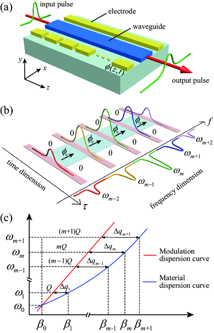
We begin with briefly illustrating synthetic (2+1) dimensions constructed in a waveguide shown in Fig. 1(a), modulated by a traveling wave with a sinusoidal radio frequency (RF) signal. The refractive index is governed by Gan and Yip (1997)
| (1) |
where is static refractive index and is the modulation amplitude. , , and are the frequency, wavevector, and modulation phase of the RF signal. For a pulse centered at the frequency propagating along the spatial dimension , the applied modulation connects field components at discrete frequencies , and forms the synthetic frequency dimension [see Fig. 1(b)] Qin et al. (2018). On the other hand, for a dispersive waveguide, the pulse experiences temporal diffraction, which brings up the concept of the synthetic dimension along the continuous retarded time frame (, with being the group velocity at ) Peschel et al. (2008); Agrawal (2010). Hence, a synthetic continuous-discrete time-frequency space is constructed for the pulse travelling along -direction inside the waveguide.
We then consider a time-dependent and spatially non-uniform modulation phase , which can be achieved by controlling RF signals at each segmented electrode. Such phase distribution supports the effective gauge potential for light in the synthetic space Fang et al. (2012). In particular, we take the form of as
| (2) |
i.e., at any , the hopping phase along the frequency dimension is in a region with the center and width , and equals to 0 at the remaining regions. Such phase distribution brings an effective gauge potential well in the synthetic space with the size dependent on [see Fig. 1(b)] Lin and Fan (2014); Lumer et al. (2019); Cohen et al. (2020), and can be used to manipulate light in different ways.
We now build detailed theoretical framework to study the system. For pulse propagating through the modulated waveguide, the electric field of the pulse can be expanded as , where is the slowly-varying envelope for the frequency component at Agrawal (2010); Boyd (2020). The propagation constant is not equally spaced due to GVD [see Fig. 1(c)], which can be defined as . Here, is the wavevector associated with , and donates the wavevector mismatching. The pulse field follows the wave equation Boyd (2020)
| (3) |
where and are vacuum and relative permittivity, respectively. With the expansion of the field, we obtain the propagating equations for component in the retarded frame sup
| (4) |
Here, is linear mismatching between light and RF signal, and is nonlinear mismatching caused by GVD, where and are Taylor expansion coefficiencies of wavevector around , representing the reciprocal of the group velocity and GVD, respectively. donates the coupling strength.
Equation (4) describes the dynamics of a pulse with multiple frequency components at propagating along -axis in a reference frame moving at . The first term on right-band side of Eq. (4) dominates the pulse dispersion behavior, which is a counterpart of wave diffusion in the spatial dimension, while the second term refers frequency conversions. Equation (4) is therefore the nonlinear Schrödinger equation within dimensions Agrawal (2010); Yuan et al. (2017), where the pulse experiences continuous temporal diffraction and discrete frequency conversion in two synthetic dimensions while it evolves at -axis [see Fig. 1(b)]. Moreover, the hopping phase in Eq. (4) gives an effective nonlinear force pointing along the frequency dimension Yuan and Fan (2016). Different from previous studies, which have explored consequences of an effective linear force in the synthetic frequency dimension Yuan and Fan (2016); Qin et al. (2018); Li et al. (2021), here the effective force is nonlinear due to GVD. Yet, as we show in the following, a synthetic time-frequency space together with the nonlinear force give us alternative opportunity for manipulating the pulse propagation in the waveguide.
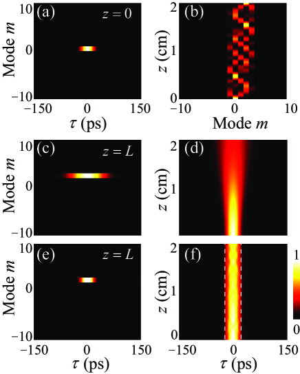
We simulate pulse propagations by Eq. (4) with excitations at one end of the waveguide at . The input pulse has a profile as , where ps is the temporal full width at half maximum (FWHM). We assume that the input field contains only one frequency component at Hz (or 1550 nm). Note that Eq. (4) is valid when the condition is satisfied, i.e., field profiles at different frequency components in the spectral domain do not overlap, where is the spectral FWHM for each frequency component at any . For the input pulse, GHz. The simulation performed with 21 modes (). Figure 2(a) shows the profile of the input pulse in the synthetic time-frequency space.
First, we consider the normal case that pulse propagates in the waveguide under the modulation with . We choose modulation with and GHz, which gives m-1. For the waveguide with a length cm, we have m-1s2, which lead to m-1. can be approximated to be zero by tuning . All parameters are chosen with the experimental feasibility in the literature Luennemann et al. (2003); Kaushalram et al. (2019); Wang et al. (2018).
When the pulse evolves along the axis, it experiences frequency conversion and nonlinear oscillation near the mode in the frequency dimension under the effective nonlinear force [see Fig. 2(b)]. At cm, frequency components of pulse oscillate back to the single mode, which shifts to the mode [see Fig. 2(c)]. Moreover, the pulse gets broadened due to GVD and has the temporal width ps, as shown in Figs. 2(c)-(d). It agrees well with the theoretical calculated evolution of the pulse width for a Gaussian pulse [see Fig. S1(a)] sup .
We next consider modulations with non-uniform distributions of phases and explore the dynamics from Eq. (4) under effective gauge potential well. We choose parameters , and ps which indicates a fixed well in the synthetic space. The simulation shows the confinement of light in middle region of the effective well (labelled by the dashed line) in the synthetic time dimension as shown in Figs. 2(e)-(f), while the frequency component is shifted to the mode as previous case. The pulse width remains 30 ps while maintaining an approximate Gaussian waveform during the propagation [see Fig. S1(b)] sup . The result here shows an interesting combination between nonlinear oscillation along the frequency dimension and the light confinement due to the effective gauge potential well in the time dimension. As a comparison, we calculate the evolution of pulse with , with other parameters unchanged, and find temporal confinement of light persists while the frequency conversion covers a broad range of modes sup . Not only the confined pulse propagation demonstrated here, the idea of utilizing effective gauge potentials in synthetic time-frequency dimensions provides more different ways to manipulate the pulse.
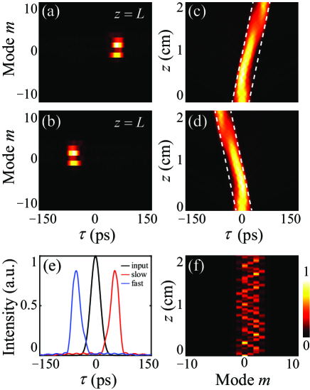
We further shift the center of the effective gauge potential well lineally dependent on with , where is the shift parameter. This choice makes the modulation phase taking the form of for ps and zero for other . It provides a way to manipulate the group velocity of pulse controlled by . In simulations, we use GHz, , and m-1s2, which give m-1, and m-1. With a positive ps/cm, we find slow light with group velocity delay of 57 ps and unchanged pulse width of 30 ps as shown in Figs. 3(a) and 3(c). On the other hand, one can see the generation of fast light in Figs. 3(b) and 3(d) with negative ps/cm. Here large dispersion and strong modulation are chosen to efficiently manipulate the group velocity of the pulse. Figure 3(e) exhibits the output pulse profiles of slow and fast light at , where the peak intensity decreases due to the dispersion loss. The corresponding nonlinear oscillation for the slow light is plotted in Fig. 3(f), while the nonlinear oscillation for the fast light is similar. At , the output pulse has two major frequency components at and modes [see Figs. 3(a)-(b)]. The single frequency conversion can be established by choosing a different propagation length. For example, one sees that oscillations shifts to a single mode at at cm. Further larger group velocity manipulation can be obtained by using larger and GVD at the cost of the intensity loss.
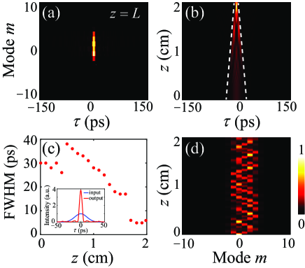
The width of effective gauge potential well can also be used to control the pulse width. We consider a varying well along with and , where is the width-varying parameter. Thus the configuration of modulation phase becomes for ps and zero for other . We take parameters ps/cm, m-1s2, and GHz, which lead to m-1 and m-1 in the simulation and show results in Fig. 4. Figure 4(a) show the pulse profile in the synthetic time-frequency space at . Although the pulse converts to multiple modes, the temporal width of the pulse is largely compressed. As shown in Fig. 4(b), the narrowing of the effective gauge potential well forces pulse compression gradually while it propagates along the axis. Figure 4(c) plots the pulse width versus , showing a trend of overall decrease. The output pulse profile has width of 5 ps, with the enhanced peak intensity. Simultaneously, the frequency conversion follows nonlinear oscillation as shown in Fig. 4(d). The output with multiple frequency components can be tuned by changing the length of the waveguide. For example, at cm, the field exhibits one major frequency component at the mode. Moreover, one can control the distribution of frequency components in the output pulse by using an input pulse with a Gaussian distribution of multiple modes. Unidirectional and bidirectional frequency transports together with temporal pulse manipulations can be achieved sup . As the last note, the pulse compression can not lead to an output field with an infinitely small temporal width (broad frequency bandwidth). The condition at any shall be satisfied.
We propose a modulated waveguide system with parameters based on lithium-niobate waveguide system. The numbers used in simulations require waveguide with large dispersion and fast electro-optic modulation, which are experimentally achievable in the second-order nonlinear waveguide with the state-of-art technology. Dispersion near m-1s2 has been reported Kaushalram et al. (2019), which can be further enlarged by structure engineering or operating at higher dispersion wavelength. corresponds to V/m voltage amplitude of an applied external electric field. If larger modulation is needed, high voltage up to 65 V/m has been demonstrated Luennemann et al. (2003). Shorter pulse manipulation is possible with smaller dispersion but larger modulation frequency, such as 100 GHz, which is commercially available Wang et al. (2018). Moreover, recent advances of integrated waveguide platform brings opportunity to achieve synthetic time-frequency dimensions in integrated photonics, on which modulators with frequency 200 GHz have been demonstrated Liu et al. (2020). The construction of a synthetic time-frequency space can be further extended beyond by adding other degrees of freedom such as orbital angular momentum Luo et al. (2015) or pseudospin Dutt et al. (2020). Besides, our analysis shall be valid for other systems if one scales parameters consistently. Our model shows promise for studying pulse propagating in dispersive resonators with synthetic dimensions Shan et al. (2020), and in third-order dispersive waveguide or microresonator based systems Hsieh et al. (2006); Mia et al. (2019); Xue et al. (2015); Yang et al. (2016).
In summary, we propose a synthetic (2+1) dimensions for manipulating pulse propagation in a dispersive waveguide under dynamic modulations. With the effective gauge potential well for photons and nonlinear oscillation in the synthetic space, multiple pulse propagation behaviors including confined pulse propagation, fast/slow light, and pulse compression have been shown. Our work provides an alternative platform for actively manipulating single pulse in different ways, which is highly re-configurable, and hence shows promising potentials for pulse engineering in integrated photonics and optical communications.
Acknowledgements.
The research is supported by National Natural Science Foundation of China (12104297, 11974245 and 12122407), National Key RD Program of China (2017YFA0303701), Shanghai Municipal Science and Technology Major Project (2019SHZDZX01), Natural Science Foundation of Shanghai (19ZR1475700), and China Postdoctoral Science Foundation (2020M671090). L. Y. acknowledges support from the Program for Professor of Special Appointment (Eastern Scholar) at Shanghai Institutions of Higher Learning. X. C. also acknowledges the support from Shandong Quancheng Scholarship (00242019024).References
- Yuan et al. (2018a) Luqi Yuan, Qian Lin, Meng Xiao, and Shanhui Fan, “Synthetic dimension in photonics,” Optica 5, 1396–1405 (2018a).
- Ozawa and Price (2019) Tomoki Ozawa and Hannah M. Price, “Topological quantum matter in synthetic dimensions,” Nat. Rev. Phys. 1, 349–357 (2019).
- Yuan et al. (2016) Luqi Yuan, Yu Shi, and Shanhui Fan, “Photonic gauge potential in a system with a synthetic frequency dimension,” Opt. Lett. 41, 741–744 (2016).
- Ozawa et al. (2016) Tomoki Ozawa, Hannah M. Price, Nathan Goldman, Oded Zilberberg, and Iacopo Carusotto, “Synthetic dimensions in integrated photonics: From optical isolation to four-dimensional quantum hall physics,” Phys. Rev. A 93, 043827 (2016).
- Bell et al. (2017) Bryn A. Bell, Kai Wang, Alexander S. Solntsev, Dragomir N. Neshev, Andrey A. Sukhorukov, and Benjamin J. Eggleton, “Spectral photonic lattices with complex long-range coupling,” Optica 4, 1433–1436 (2017).
- Qin et al. (2018) Chengzhi Qin, Feng Zhou, Yugui Peng, Dimitrios Sounas, Xuefeng Zhu, Bing Wang, Jianji Dong, Xinliang Zhang, Andrea Al, and Peixiang Lu, “Spectrum control through discrete frequency diffraction in the presence of photonic gauge potentials,” Phys. Rev. Lett. 120, 133901 (2018).
- Luo et al. (2015) Xiwang Luo, Xingxiang Zhou, Chuanfeng Li, Jinshi Xu, Guangcan Guo, and Zhengwei Zhou, “Quantum simulation of 2d topological physics in a 1d array of optical cavities,” Nat. Commun. 6, 1–8 (2015).
- Regensburger et al. (2011) Alois Regensburger, Christoph Bersch, Benjamin Hinrichs, Georgy Onishchukov, Andreas Schreiber, Christine Silberhorn, and Ulf Peschel, “Photon propagation in a discrete fiber network: An interplay of coherence and losses,” Phys. Rev. Lett. 107, 233902 (2011).
- Regensburger et al. (2012) Alois Regensburger, Christoph Bersch, Mohammad-Ali Miri, Georgy Onishchukov, Demetrios N Christodoulides, and Ulf Peschel, “Parity–time synthetic photonic lattices,” Nature 488, 167–171 (2012).
- Lustig et al. (2019) Eran Lustig, Steffen Weimann, Yonatan Plotnik, Yaakov Lumer, Miguel A. Bandres, Alexander Szameit, and Mordechai Segev, “Photonic topological insulator in synthetic dimensions,” Nature 567, 356–360 (2019).
- Maczewsky et al. (2020) Lukas J. Maczewsky, Kai Wang, Alexander A. Dovgiy, Andrey E. Miroshnichenko, Alexander Moroz, Max Ehrhardt, Matthias Heinrich, Demetrios N. Christodoulides, Alexander Szameit, and Andrey A. Sukhorukov, “Synthesizing multi-dimensional excitation dynamics and localization transition in one-dimensional lattices,” Nat. Photonics 14, 76–81 (2020).
- Wang et al. (2020) Kai Wang, Bryn A. Bell, Alexander S. Solntsev, Dragomir N. Neshev, Benjamin J. Eggleton, and Andrey A. Sukhorukov, “Multidimensional synthetic chiral-tube lattices via nonlinear frequency conversion,” Light Sci. Appl. 9, 132 (2020).
- Yuan and Fan (2016) Luqi Yuan and Shanhui Fan, “Bloch oscillation and unidirectional translation of frequency in a dynamically modulated ring resonator,” Optica 3, 1014–1018 (2016).
- Luo et al. (2018) Xi Wang Luo, Chuanwei Zhang, Guang Can Guo, and Zheng Wei Zhou, “Topological photonic orbital-angular-momentum switch,” Phys. Rev. A 97, 043841 (2018).
- Yuan et al. (2018b) Luqi Yuan, Qian Lin, Meng Xiao, Avik Dutt, and Shanhui Fan, “Pulse shortening in an actively mode-locked laser with parity-time symmetry,” APL Photonics 3, 086103 (2018b).
- Yang et al. (2020) Zhaoju Yang, Eran Lustig, Gal Harari, Yonatan Plotnik, Yaakov Lumer, Miguel A. Bandres, and Mordechai Segev, “Mode-locked topological insulator laser utilizing synthetic dimensions,” Phys. Rev. X 10, 011059 (2020).
- Yuan et al. (2019) Luqi Yuan, Qian Lin, Anwei Zhang, Meng Xiao, Xianfeng Chen, and Shanhui Fan, “Photonic gauge potential in one cavity with synthetic frequency and orbital angular momentum dimensions,” Phys. Rev. Lett. 122, 083903 (2019).
- Dutt et al. (2020) Avik Dutt, Qian Lin, Luqi Yuan, Momchil Minkov, Meng Xiao, and Shanhui Fan, “A single photonic cavity with two independent physical synthetic dimensions,” Science 367, 59–64 (2020).
- Reeves et al. (2003) W. H. Reeves, Dmitry V Skryabin, Fabio Biancalana, Jonathan C. Knight, P. St. J. Russell, F. G. Omenetto, Anatoly Efimov, and A. J. Taylor, “Transformation and control of ultra-short pulses in dispersion-engineered photonic crystal fibres,” Nature 424, 511–515 (2003).
- Huang et al. (2015) S. W. Huang, H. Zhou, J. Yang, J. F. McMillan, A. Matsko, M. Yu, D. L. Kwong, L. Maleki, and C. W. Wong, “Mode-locked ultrashort pulse generation from on-chip normal dispersion microresonators,” Phys. Rev. Lett. 114, 053901 (2015).
- Divitt et al. (2019) Shawn Divitt, Wenqi Zhu, Cheng Zhang, Henri J. Lezec, and Amit Agrawal, “Ultrafast optical pulse shaping using dielectric metasurfaces,” Science 364, 890–894 (2019).
- Stratmann et al. (2005) M. Stratmann, T. Pagel, and F. Mitschke, “Experimental observation of temporal soliton molecules,” Phys. Rev. Lett. 95, 143902 (2005).
- Lee et al. (2017) Seung Hoon Lee, Dong Yoon Oh, Qi Fan Yang, Boqiang Shen, Heming Wang, Ki Youl Yang, Yu Hung Lai, Xu Yi, Xinbai Li, and Kerry Vahala, “Towards visible soliton microcomb generation,” Nat. Commun. 8, 1–8 (2017).
- Broderick et al. (1997) N. G. R. Broderick, D. Taverner, D. J. Richardson, M. Ibsen, and R. I. Laming, “Optical pulse compression in fiber bragg gratings,” Phys. Rev. Lett. 79, 4566–4569 (1997).
- Colman et al. (2010) Pierre Colman, Chad Husko, Sylvain Combrié, Isabelle Sagnes, Chee Wei Wong, and Alfredo De Rossi, “Temporal solitons and pulse compression in photonic crystal waveguides,” Nat. Photonics 4, 862 (2010).
- Tan et al. (2010) Dawn T. H. Tan, Pang C. Sun, and Yeshaiahu Fainman, “Monolithic nonlinear pulse compressor on a silicon chip,” Nat. Commun. 1, 1–6 (2010).
- Gehring et al. (2006) George M. Gehring, Aaron Schweinsberg, Christopher Barsi, Natalie Kostinski, and Robert W. Boyd, “Observation of backward pulse propagation through a medium with a negative group velocity,” Science 312, 895–897 (2006).
- Li et al. (2015) Guangzhen Li, Yuping Chen, Haowei Jiang, Yi’an Liu, Xiao Liu, and Xianfeng Chen, “Tunable temporal gap based on simultaneous fast and slow light in electro-optic photonic crystals,” Opt. Express 23, 18345–18350 (2015).
- Qin et al. (2020) Tian Qin, Jianfan Yang, Fangxing Zhang, Yao Chen, Dongyi Shen, Wei Liu, Lei Chen, Xiaoshun Jiang, Xianfeng Chen, and Wenjie Wan, “Fast-and slow-light-enhanced light drag in a moving microcavity,” Commun. Phys. 3, 1–8 (2020).
- Agrawal (2010) G. P. Agrawal, Nonlinear Fiber Optics, Optics and Photonics (Elsevier Science, 2010).
- Peschel et al. (2008) Ulf Peschel, Christoph Bersch, and Georgy Onishchukov, “Discreteness in time,” Centr. Eur. J. Phys. 6, 619–627 (2008).
- Plansinis et al. (2015) B. W. Plansinis, W. R. Donaldson, and G. P. Agrawal, “What is the temporal analog of reflection and refraction of optical beams?” Phys. Rev. Lett. 115, 183901 (2015).
- Plansinis et al. (2016) Brent W. Plansinis, William R. Donaldson, and Govind P. Agrawal, “Temporal waveguides for optical pulses,” J. Opt. Soc. Am. B 33, 1112–1119 (2016).
- Lin and Fan (2014) Qian Lin and Shanhui Fan, “Light guiding by effective gauge field for photons,” Phys. Rev. X 4, 031031 (2014).
- Lumer et al. (2019) Yaakov Lumer, Miguel A. Bandres, Matthias Heinrich, Lukas J. Maczewsky, Hanan Herzig-Sheinfux, Alexander Szameit, and Mordechai Segev, “Light guiding by artificial gauge fields,” Nat. Photonics 13, 339–345 (2019).
- Cohen et al. (2020) Moshe Ishay Cohen, Christina Jörg, Yaakov Lumer, Yonatan Plotnik, Erik H. Waller, Julian Schulz, Georg von Freymann, and Mordechai Segev, “Generalized laws of refraction and reflection at interfaces between different photonic artificial gauge fields,” Light Sci. Appl. 9, 200 (2020).
- Gan and Yip (1997) F. Y. Gan and G. L. Yip, “Traveling wave electrode design for high speed mach-zehnder linbo3 intensity modulators,” in Applications of Photonic Technology 2 (Springer, 1997) pp. 469–475.
- Fang et al. (2012) Kejie Fang, Zongfu Yu, and Shanhui Fan, “Realizing effective magnetic field for photons by controlling the phase of dynamic modulation,” Nat. Photonics 6, 782–787 (2012).
- Boyd (2020) Robert W. Boyd, Nonlinear optics (Academic press, 2020).
- (40) See Supplemental Material at http://link.aps.org/ for more details on the derivation of the pulse-propagation equations and additional simulation results.
- Yuan et al. (2017) Luqi Yuan, Da Wei Wang, and Shanhui Fan, “Synthetic gauge potential and effective magnetic field in a raman medium undergoing molecular modulation,” Phys. Rev. A 95, 033801 (2017).
- Li et al. (2021) Guangzhen Li, Yuanlin Zheng, Avik Dutt, Danying Yu, Qingrou Shan, Shijie Liu, Luqi Yuan, Shanhui Fan, and Xianfeng Chen, “Dynamic band structure measurement in the synthetic space,” Sci. Adv. 7, eabe4335 (2021).
- Luennemann et al. (2003) M. Luennemann, U. Hartwig, G. Panotopoulos, and K. Buse, “Electrooptic properties of lithium niobate crystals for extremely high external electric fields,” Appl. Phys. B 76, 403–406 (2003).
- Kaushalram et al. (2019) A. Kaushalram, S. A. Samad, G. Hegde, and S. Talabattula, “Tunable large dispersion in hybrid modes of lithium niobate-on-insulator multimode waveguides,” IEEE Photon. J. 11, 1–8 (2019).
- Wang et al. (2018) Cheng Wang, Mian Zhang, Xi Chen, Maxime Bertrand, Amirhassan Shams-Ansari, Sethumadhavan Chandrasekhar, Peter Winzer, and Marko Lončar, “Integrated lithium niobate electro-optic modulators operating at cmos-compatible voltages,” Nature 562, 101–104 (2018).
- Liu et al. (2020) Xuecheng Liu, Bing Xiong, Changzheng Sun, Zhibiao Hao, Lai Wang, Jian Wang, Yanjun Han, Hongtao Li, Jiadong Yu, and Yi Luo, “Thin film lithium niobate electro-optic modulator based on a slow wave structure,” in Conference on Lasers and Electro-Optics/Pacific Rim (Optical Society of America, 2020) p. C4C_3.
- Shan et al. (2020) Qingrou Shan, Danying Yu, Guangzhen Li, Luqi Yuan, and Xianfeng Chen, “One-way topological states along vague boundaries in synthetic frequency dimensions including group velocity dispersion.” Prog. Electromagn. Res. 169 (2020).
- Hsieh et al. (2006) I-Wei Hsieh, Xiaogang Chen, Jerry I. Dadap, Nicolae C. Panoiu, Richard M. Osgood, Sharee J. McNab, and Yurii A. Vlasov, “Ultrafast-pulse self-phase modulation and third-order dispersion in si photonic wire-waveguides,” Opt. Express 14, 12380–12387 (2006).
- Mia et al. (2019) Md Borhan Mia, Nafiz Jaidye, and Sangsik Kim, “Extremely high dispersions in heterogeneously coupled waveguides,” Opt. Express 27, 10426–10437 (2019).
- Xue et al. (2015) Xiaoxiao Xue, Yi Xuan, Yang Liu, Pei-Hsun Wang, Steven Chen, Jian Wang, Dan E Leaird, Minghao Qi, and Andrew M Weiner, “Mode-locked dark pulse kerr combs in normal-dispersion microresonators,” Nat. Photonics 9, 594–600 (2015).
- Yang et al. (2016) Ki Youl Yang, Katja Beha, Daniel C. Cole, Xu Yi, Pascal Del’Haye, Hansuek Lee, Jiang Li, Dong Yoon Oh, Scott A. Diddams, Scott B. Papp, and Kerry J. Vahala, “Broadband dispersion-engineered microresonator on a chip,” Nat. Photonics 10, 316–320 (2016).