SIR Coverage Analysis in Cellular Networks with Temporal Traffic: A Stochastic Geometry Approach
Abstract
The bloom in mobile applications not just bring in enjoyment to daily life, but also imposes more complicated traffic situation on wireless network. A complete understanding of the impact from traffic profile is thus essential for network operators to respond adequately to the surge in data traffic. In this paper, based on stochastic geometry and queuing theory, we develop a mathematical framework that captures the interplay between the spatial location of base stations (BSs), which determines the magnitude of mutual interference, and their temporal traffic dynamic. We derive a tractable expression for the SIR distribution, and verify its accuracy via simulations. Based on our analysis, we find that ) under the same configuration, when traffic condition changes from light to heavy, the corresponding SIR requirement can differ by more than 10 dB for the network to maintain coverage, ) the SIR coverage probability varies largely with traffic fluctuation in the sub-medium load regime, whereas in scenario with very light traffic load, the SIR outage probability increases linearly with the packet arrival rate, ) the mean delay, as well as coverage probability of cell edge user equipments (UEs) are vulnerable to the traffic fluctuation, thus confirms its appeal for traffic-aware communication technology.
Index Terms:
Poisson point process, cellular networks, random packet arrival, interacting queues, stochastic geometry, mean delay.I Introduction
The rapid evolution of mobile applications imposes more complicated traffic condition on wireless networks, where not only the data demand grows exponentially [LopDinCla:15], but more importantly, the the content is largely changing from mobile voice to multimedia [niu2011tango]. To give an adequate response to the surge in mobile data traffic, network operators need a complete understanding on the impact of temporal traffic. In this article, we aim to evaluate how the traffic statistic affects the wireless networks, and to find those aspects that are most vulnerable.
I-A Background and Related Work
Due to the broadcast nature of wireless channel, transmitters in space sharing a common spectrum will interact with each other through the interference they cause. To characterize the performance of such networks, stochastic geometry has been recently introduced as a way to assess performance of wireless links in large-scale networks [HaeAndBac:09, Hae:12, BacBla:09, ElSHosHae:13, ElSSulAlo:17, DiLuGua:16]. The intrinsic elegance in modeling and analysis has popularized its application in evaluating performance among various wireless systems, including ad-hoc networks [HaeAndBac:09], cellular networks [AndBacGan:11], or more advanced heterogeneous networks [DhiGanBac:12], even with device-to-device (D2D) communication [YanLeeQue:16] and multiple-input multiple-output (MIMO) technology [YanGerQue:16, YanGerQue:17]. However, the main drawback of these models is that they heavily rely on the full buffer assumption, i.e., every link always has a packet to transmit, and do not allow one to represent random traffic. While the additional dimension of randomness in temporal domain increases the complexity in analysis, it is nevertheless a crucial factor in understanding network performance, especially for the next generation wireless system that faces more voliated traffic conditions [ZhoHaeZhe:16, AndBuzCho:14].
The main difficulty with queuing in wireless network comes from the interdependency among the evolution of different queues, which is usually referred to as interacting queues [rao1988stability]. Because of interference, the queue status of one transmitter can affect, and also be affected by, the queue status of its neighbors, hence making the analysis very difficult. Conventionally, the queuing interaction through wireless medium is studied using simple collision models [BerGalHum:92, rao1988stability, LuoEph:99, BorMcDPro]. In such models, discrete time ALOHA protocol is usually employed, where each of the terminals initiates a transmission attempt at every slot: If more than two terminals transmit simultaneously, a collision occurs and all the terminals retransmit their packets in next slot with the same probability [BerGalHum:92]. Analytical results about system stability can be obtained via exact form in scenarios with few (two or three) transmitters [rao1988stability], or through approximations in asymptotic regime with infinitely many transmitters [BorMcDPro:12]. However, these models over simplify the wireless channel and lack the ability to tract the interference, which differs according to distance as well as channel gains, thus do not capture the information-theoretic interactions precisely. Recent attempts to address this issue are made in [ZhoQueGe:16, GhaElsBad:17, yang2017packet, ZhoHaeQue:16, GeoSpyKal:17], where queuing theory is combined with stochastic geometry to model the dynamic from both temporal and spatial domains. The results provide the necessary and sufficient conditions for network to be stable [ZhoHaeQue:16], and different performance metrics, including success transmission probability [GhaElsBad:17], delay [ZhoQueGe:16], and packet throughput [yang2017packet] have been subsequently derived. While giving more refined analysis, these results either provide only bounds that are not necessary tight [ZhoQueGe:16, ZhoHaeQue:16], or are only appliable to networks with light traffic [yang2017packet]. The most related work is from [GhaElsBad:17], where the authors applied Geo/PH/1 queuing model to account for the interference-based queues among UEs and analyzed the SIR performance under three different transmission schemes. However, the requirement for full channel inversion limits its generalization, and the restricted stable region constrains its application to relatively low traffic condition with small SIR detection threshold, and thus prevents one to take a complete treatment on traffic statistic. To this end, a mathematical framework that captures the spatial–temporal dynamic of the network, and adapts to scenarios with different traffic conditions is of necessity to be explored.
I-B Approach and Summary of Contributions
In this paper, we model the BS deployment and UE locations as independent Poisson point processes (PPPs), where each BS maintains an infinite capacity buffer to store the incoming packets. The queuing dynamic is modelled via a descrete time system, where we consider the arrival of packets at each BS to be independent Bernoulli process. By combining stochastic geometry with queuing theory, we obtain a tractable expression for the SIR coverage probability. With the developed framework, we can explicitly characterize the SIR variation due to change of traffic condition, and its consequential impact on system stability, as well as delay distribution. Our main contributions are summarized below.
-
•
We develope a mathematical framework that captures the interplay between the spatial geometry of wireless links and their temporal traffic dynamic. Our analysis is tractable, and takes into account all the key features of a cellular network, including traffic profile, small-scale fading and path loss, random network topology, and queuing interaction.
-
•
Unlike [GhaElsBad:17], our result not only provides the standard SIR coverage probability, but also gives a more precise description about the fraction of UEs achieving SIR at different levels. For instance, the SIR coverage probability of cell-edge UEs can be easily derived via our result.
-
•
We discuss the sufficient and necessary conditions for the network to be stable, and provide an approximation for the stable region. We also derive the mean delay distribution, by accounting for both queuing and transmission delay.
-
•
Using the developed analysis, we find that under the same network configuration, there is more than 10 dB SIR difference between light and heavy traffic conditions. Moreover, in the very light traffic regime, the network SIR outage probability is shown to increase linearly with packet arrival rate. The result also reveals that the mean delay, as well as cell-edge UE rate, are vulnerable to the variation of traffic condition, hence urging advanced solution to adapt with traffic profile.
The remainder of the paper is organized as follows. We introduce the system model in Section II. In Section III, we detail the analysis of SIR distribution in cellular networks with temporal traffic. We show the simulation and numerical results in Section LABEL:sec:NumAnal, that confirm the accuracy of our analysis, and provide insights about the impact of traffic profile on network performance. We conclude the paper in Section LABEL:sec:conclusions.
II System Model
In this section, we provide a general introduction to the network topology, the traffic profile, as well as the propagation and failure retransmission model. The main notations used throughout the paper are summarized in Table I.
| Notation | Definition |
|---|---|
| ; | PPP modeling the location of base stations; BS deployment density |
| ; | PPP modeling the location of UEs; UE deployment density |
| ; | BS transmit power; path loss exponent |
| -stable region of wireless network, under which the fraction of unstable queues is less than | |
| ; | Packet arrival rate; critical arrival rate for -stability |
| ; | Received SIR of typical UE at time slot ; SIR decoding threshold |
| Conditional SIR coverage probability at time slot |
II-A Network Topology and Traffic Model
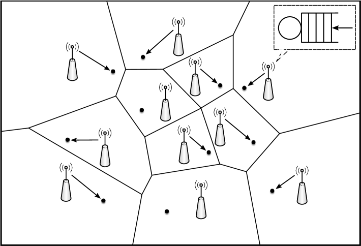
We consider the downlink of a cellular network, as depicted in Fig. 1, that consists of randomly deployed BSs whose spatial locations follow independent Poisson point process (PPP) with spatial densities .111PPPs serve as a good model for the planned deployment of macro cell BSs, as verified by both empirical evidence [TayDhiNov:12, DiLuGua:16] and theoretical analysis [BlaKarKee:13]. The location of UEs is modelled as another independent PPP with spatial density , where each UE associates with its closest BS for transmission. We assume the UE density is high enough that every BS has at least one UE associates with it.222The one UE per cell set up is mainly for the sake of notational simplicity. By adopting a similar approach as [yang2017packet], the analysis in this paper can be easily extended to consider more realistic scenario where multiple UEs in each cell share the same wireless channel. In this network, all BSs and UEs are assumed to be equipped with single antenna, and each BS transmits with constant power . In light of its spectral efficiency, we employ universal frequency reuse throughout the network, i.e., every BS transmits in the same spectrum.
We use a discrete time queuing system to model the random traffic profile. In particular, the time axis is segmented into a sequence of equal time intervals, referred to as time slots. We further assume all queuing activities, i.e., arrivals and departures, take place around the slot boundaries. Specifically, at the time slot, a potential packet departure may occur in the interval , and a potential packet arrival can happen in the interval . In other words, departures occur at the moment immediately before the slot boundaries while arrivals occur at the moment immediately after the slot boundaries. For a generic UE located in the cell of , we model its packet arrival as a Bernoulli process with rate , which represents the probability of a new arrival occurs in a slot. We further assume that each BS accumulates all the incoming packets in an infinite-size buffer for further transmission purpose.
In order to investigate the evolution of queuing dynamic, we limit the mobility of transceivers by considering a static network, i.e., the locations of the BSs and UEs are generated once at , and remained unchanged in all the following time slots.333Note that most of the pratical networks can be approximately regarded as static, since the locations of any end device cannot change drastically in a relatively short period [ZhoHaeQue:16].
II-B Propagation Channel and Failure Retransmission
In this network, we adopt a block-fading propagation model, where the channels between any pair of antennas are assumed independent and identically distributed (i.i.d.) and quasi-static, i.e., the channel is constant during one transmission slot, and varies independently from slot to slot. We consider all propagation channels are narrowband and affected by two attenuation components, namely small-scale Rayleigh fading with unit mean power, and large-scale path loss that follows power law.444The analysis in this paper is not necessary constrained to simple propagation model, it can be further extended to incorporate more realistic setups that include multi-slope path loss [DinWanLop:16, AndZhaDur:16] and complicated fading environment [ChuCotDhi:17, TriAffLia:17].
Affected by the random channel fading and aggregated interference, the process of packet departure does not possess a constant rate and can lead to failure packet deliverty. Retransmission is thus necessary to guarantee the packet can be correctly received. By enabling retransmission, the transmission model at each BS becomes: During each time slot, every node with a non-empty buffer sends out a packet from the head of its queue. If the received SIR exceeds a predefined threshold, the transmission is successful and the packet can be removed from the queue; otherwise, the transmission fails and the packet remains in the buffer. We assume the feedback of each transmission, either success or fail, can be instantaneously awared by the BSs such that they are able to schedule transmission at next time slot. Moreover, for the BSs with empty buffer, they mute the transmissions to reduce power consumption and inter-cell interference.
II-C Signal-to-interference ratio (SIR)
By applying Slivnyak’s theorem [BacBla:09] to the stationary PPP of BS, it is sufficient to focus on the SIR of a typical UE at the origin, with its tagged BS located at . Given the UE is receiving data at time slot , the received SIR can be written as
| (1) |
where denotes the small scale Rayleigh fading from BS to the origin, is the Euclidean distance, stands for the path loss exponent, and is an indicator showing whether a node located at is transmitting at time slot () or not ().
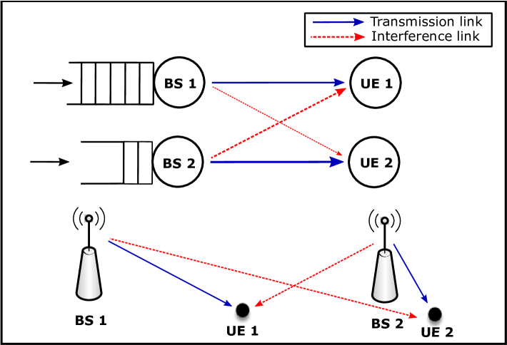
It is important to note that since the spectrum is shared among BSs, the queuing status of each BS is coupled with other transmitters and hence results in interacting queue. As such, the BS active state, , is both spatial and temperal dependent, since the location affects the pathloss and further the aggregated interference, and the time changes the queue length at each node. To better illustrate this concept, Fig. 2 gives a simple example of queuing interaction between two BSs. Note that compared to UE 1, UE 2 has an advantage location and hence enjoys better path loss and fewer interference. Consequently, BS 2 can quickly empty its queue, and the disparity between their communication conditions results in BS 2 activates less frequently than BS 1. Moreover, depending on whether packets appear at both BSs or not, the corresponding active durations are also different: If both transmitters have packets to send, the mutual interference will reduce the service rate and prolong the active duration of each BS individually. On the other hand, when one transmitter becomes silent, the other one can benefit from the reduced cross-talk and speed up its queue flushing process, hence also decreases the active period. Extending this concept to a large-scale network, we find that as the realization of PPP is irregular, there are always some BSs experience poor transmission environment, e.g., their UEs are located at the cell edge, and some others having good communication condition, e.g., their UEs are around the cell centers. In this regard, even the packet arrival rate is the same for all transmitters, the queuing status and active state can varies largely from BS to BS, and the characterization of SIR in such network is very challenging.
III Analysis
| (4) |
We now present the main technical results of the paper. In particular, we first detail the definition of conditional SIR coverage probability, and the analysis on its distribution. Then we discuss the conditions for the queuing network to be stable. After that, we give moments as well as a computationally efficient approximation for the conditional SIR coverage probability. Finally, we derive the distribution of mean delay, which involves both queuing and transmission delay.
III-A Conditional SIR Coverage Probability
Since both the received signal strength and the interference at a given UE are governed by a number of stochastic processes, e.g., random spatial distribution of transmitting/receiving nodes, random packet arrivals, and queuing dynamics, the SIR in (1) is a random variable and can only be characterized via distribution. In this regard, conditioning on the realization of the point process , we define the conditional SIR coverage probability as follows [haenggi2016meta, ZhoHaeQue:16].
Definition 1
Given the typical UE is receiving data at time slot ,, its conditional SIR coverage probability is defined as
| (2) |
Note that the conditional SIR coverage probability is still a random variable (as we condition on the realization of ), which contains all the information about the UE SIR (and therefore achievable rate) distribution across the network. Moreover, the interaction of queues is also captured by (1) via the accumulated interference.
In order to analyze the distribution of , we need to address two issues: ) due to random packet arrival and retransmission of failed deliveries, the active state, i.e., , at each transmitter varies over time, and ) there may exist common interferencing BSs seen by the same UE from one time slot to another, which introduces temporal correlation for the SIR coverage probability [SchBetBra:12, ZhoZhaHae:14, GanHae:09]. The dynamically changing active state of BSs, together with the temperal correlation, involve memory to the queues and highly complicates the analysis. Fortunately, when the number of transmitters asymptotically approaches infinity, a mean field property starts to emerge in the evolution of queues, i.e., the interaction between queues become “weak” and “global”, and the impact from aforementioned temperal and spatial correlation tends to be negligible on the employed system model [BorMcDPro].555The mean field effect appears because of the cellular infrastruture, where interference is bounded away from the tagged transmitter. In Poisson bipolar networks, where the interaction is “strong” and “local”, such approximation may not hold. Motivated by this fact, we make the following assumption.
Assumption 1
The temporal interference correlation has a negligible effect on the transmission SIR coverage probability. Hence, we assume the typical UE sees almost independent interference at each time slot.
It is now safe to assume that all UEs experience i.i.d. steady state queue distributions, and each BS activates independently, whereas the active probability depends on the specific service rate, or equivalently, the SIR coverage probability. To faciliate analysis in the following, we introduce a simple result from queuing theory as a preliminary, which describes the active probability of a transmitter under fixed arrival and departure rates.
Lemma 1
Given the arrival rate being , the service rate , the active probability at a generic BS is
| (5) |
Proof:
The result is a standard conclusion from Geo/Geo/1 queue, which can be found in [AteMor:04]. ∎
After all the above preparason, we are now ready to derive our main result of this paper, i.e., distribution of the conditional SIR coverage probability.
Theorem 1
The cumulative distribution function of the conditional SIR coverage probability is given by the fixed-point equation (4) on top of this page, which can be iterative solved as follows
| (5) |
where is given by
| (6) |
whereas , denotes the imaginary part of a complex number, and has the form as
| (7) |
with being the hypergeometry function [AndAsk:00], and is given as
| (8) |
In particular, when , we have .
Proof:
See Appendix LABEL:appnd:_Prf_Dist_ConProb_ExaC. ∎
The expression in (4) not only quantifies how all the key features of a cellular network, i.e., deployment strategy, interference, and traffic profile, affect the distribution of SIR, but also illustrates how the interacting queues are affecting the SIR coverage via a fixed-point functional equation. The function can be interpreted from two aspects: If we regard a typical cell as a queuing system, equation (4) describes the distribution of the random service rate; if we look at (4) in the view of network performance, then the CCDF, i.e., , gives the level of certainty that at least fraction of UEs in the network can attain SIR threshold . Several numerical results based on (4) will be shown in Section IV to provide more practical insights. In the following, we discuss the stable region, moments of the conditional SIR coverage probability, and approximation for the CDF.
Remark 1
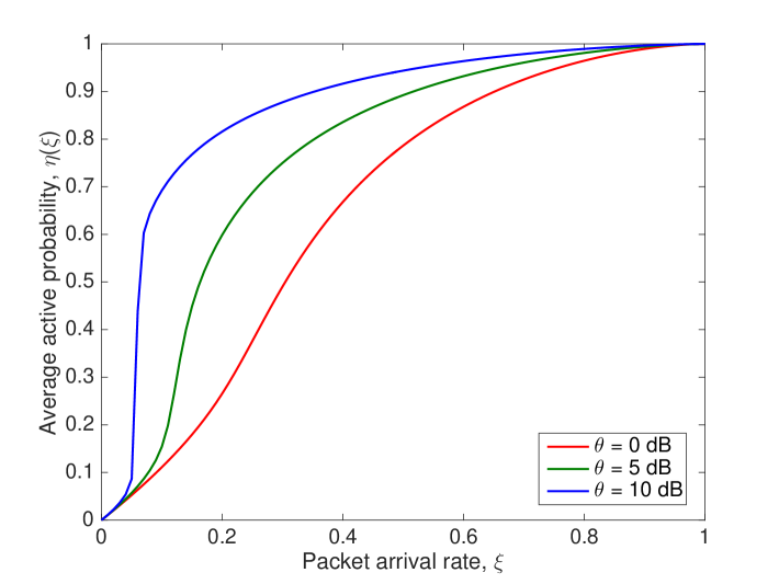
We introduce an auxiliary function as
| (9) |
which can be regarded as “average” active probability. Note that as grows from 0 to 1, while the value of also variates accordingly, the trend is very different. As depicted in Fig. 3, we can see that, with failed packet retransmissions, the average active probability goes up on a fast-and-then-slow basis with respect to the packet arrival rate , and this effect is especially significant in networks with high SIR detection threshold.
III-B Stable Region
The primal consideration in queuing systems is about stability, i.e., the critical conditions under which all the queues can remain finite length and do not explode. For an isolated system, even with random arrival and departure process, the stable region can be explicitly determined to be when average service rate is larger than the average arrival rate (Loynes theorem [Loy:62]). However, such condition cannot be directly generalized to large-scale queuing networks, as the strict stability, i.e., all queues are finite-length, is not achievable (except for the trivial case of ). Recall our discussion in Section II, the random locations of both BS and UE always result in some UEs located at poor coverage area, e.g., the cell edge, and having unbounded queue length. In this regard, instead of requiring all the queues to be stable, a more meaningful alternative will be to maintain the fraction of unstable queues to be below certain level. To this end, we introduce the -stable region [ZhoHaeQue:16], which gives the conditions for a network to be operated with less than portion of saturated queues. Following [ZhoHaeQue:16], a formal definition is in the sequel.
Definition 2
For any , the - stable region and the critical arrival rate are defined respectively as
| (10) |
and
| (11) |
The network is -stable if and only if .
The critical arrival rate gives an explicit stable boundary, beyond which there are more queues transfering from finite size to infinite length and the requirement of less than portion of unstable queues cannot be guaranteed. While an exact expression for the critical arrival rate is not available, we can nevertheless obtain explicit conditions for the network to be -stable.
Theorem 2
The sufficient condition for the network to be -stable is
| (12) |
and the necessary condition for the network to be -stable is
| (13) |
Proof:
For the sufficient condition, we consider a dominant system, where all the nodes keep transmitting irrespect of their buffer status (for a node with empty buffer, it transmits “dummy” packets). As such, the interference in dominant system is larger than the actual ones, and the result can be attained via having in (4).
For the necessary condition, we consider a favorable system, where each node transmits without retransmission, i.e., even there is transmission failure, the transmitter simplily ignores the failure and withdraw the failed packets. In this scenario, the interference is smaller than that of the actual one, whereas we can obtain the result as making . ∎
From the above results, we note that the actual value of the critical arrival rate falls in the interval of . Using the ergodic property of PPP, an approximation for the -stable region is given in the sequel.
Corollary 1
The -stable region of the network is approximated as follows
| (14) |
Proof:
Note that due to stationary and ergodicity, the ensemble average obtained by averaging over the point process equals the spatial averages obtained by averaging an arbitrary realization of PPP over a large region, i.e.,
| (15) |
and the result follows according to the definition. ∎