Site-Specific Deployment Optimization of Intelligent Reflecting Surface for Coverage Enhancement

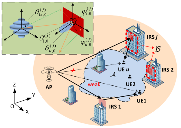
As shown in Fig. 1, the AP is located on the Z-axis of the cartesian coordinate system, with a height of $H_{\textrm{AP}}$. Distributed IRSs are installed on building surfaces to assist the AP in communicating with ground UEs, which are located in a target area $\mathcal{A}$ with site-specific blockages. For simplicity and the purpose of illustration, buildings are modeled as cuboids with random heights. Each IRS is assumed to be a uniform planar array (UPA) with $N\triangleq N_{\textrm{h}}\times N_{\textrm{v}}$ elements. The spacing of the elements along the horizontal and vertical direction are $d_{\textrm{h}}$ and $d_{\textrm{v}}$, respectively, whose values are usually between $\frac{\lambda}{10}$ and $\frac{\lambda}{2}$ [14], where $\lambda$ is the signal wavelength. The entire candidate area on the building surfaces for IRS deployment is denoted as $\mathcal{B}$. The actual deployment location of the IRS $j$ is denoted as $w_{j}\in\mathcal{B},j\in\mathcal{J}\triangleq\{1,\cdots,J\}$.

The coordinate of typical UE $u\in\mathcal{U}\triangleq\{1,\cdots,U\}$, in ground area $\mathcal{A}$ is expressed as $\mathbf{g}_{u}\triangleq\left[u_{\textrm{x}},u_{\textrm{y}},H_{\textrm{u}}\right]^{T}$. Taking the position of the central element as the IRS reference point, then the coordinate of the IRS $j$ reference coordinate is denoted by ${\mathbf{q}}_{j}\triangleq[x_{j},y_{j},z_{j}]^{T}$.

When considering the isotropic radiation patterns on the AP and IRS sides, the channel amplitude from AP to the element $n$ of IRS $j$ can be expressed as[9]

where $g_{\textrm{i}}^{(j)}$ denotes the average channel power gain, $\xi_{\textrm{i},n}^{(j)}$ accounts for channel fading and can be modeled as a random variable (RV) that characterizes the multi-path fading effect. For simplicity, we assume half-wavelength spacing between elements. Then the fading terms $\xi_{\textrm{i},n}^{(j)}$ can be considered as independent and identically distributed (i.i.d.), which follow the Rician distribution with a mean power of ${\mathbb{E}\{|{\xi}_{\textrm{i},n}^{(j)}|^{2}\}}=1$ and the Rician K-factor ${K_{\textrm{i}}^{(j)}}$.

When the non-isotropic radiation patterns of AP and IRS are considered, the expression for channel amplitude becomes

The Rician factor of new channel fading becomes $\tilde{K}_{\textrm{i}}^{(j)}$, and the mean power becomes $\mathbb{E}\{|\tilde{\xi}_{\textrm{i},n}^{(j)}|^{2}\}$. To describe the variation of small-scale fading, we respectively define the gain of the Rician factor $G_{K_{\textrm{i}}^{\textrm{(j)}}}$ and the mean fading power gain $\rho_{\textrm{i}}^{\textrm{(j)}}$ as

Drawing upon reference[9] and [16], we further derive the following expressions. The Rician factor gain and mean fading power gain can be respectively expressed as

and

In the formulas, $E_{\textrm{i,NLoS}}^{(j)}$ is the mean power of the NLoS component when non-isotropic antennas are considered, ${F^{\textrm{tx}}}({\theta_{{\rm{tx,0}}}^{(j)}})$ and ${F^{\textrm{i}}}({\Omega_{{\rm{i,0}}}^{(j)}})$ represent the values of TX and RX along the LoS direction, respectively. Here, ${\theta_{{\rm{tx,0}}}^{(j)}}$ denotes the elevation angle of the LoS direction of departure (DoD) for the AP, while ${\Omega_{{\rm{i,0}}}^{(j)}}\triangleq(\theta_{{\rm{i,0}}}^{(j)},\varphi_{{\rm{i,0}}}^{(j)})$ specifies the LoS direction of arrival (DoA) at the IRS.

Ground UEs are equipped with an isotropic antenna with unit antenna gain. Similarly, when considering the isotropic radiation patterns at both IRS and UE sides, the channel amplitude from the element $n$ of IRS $j$ to UE $u$ is given by

where, $g_{\textrm{r,u}}^{(j)}$ denotes the average channel power gains, $\xi_{\textrm{r},n,u}^{(j)}$ account for channel fading. When the non-isotropic radiation pattern of IRS is considered, the expression for channel amplitude becomes

corresponding Rician factor gain $G_{K_{\textrm{r},u}^{\textrm{(j)}}}$ and average fading power gain $\rho_{\textrm{r},u}^{\textrm{(j)}}$ can be respectively expressed as

and

where, ${\Omega_{{{u,0}}}^{(j)}}\triangleq(\theta_{{{u,0}}}^{(j)},\varphi_{{{u,0}}}^{(j)})$ denotes the LoS DoD at the IRS.

Based on the above model and analysis, by considering non-isotropic radiation patterns at the AP and IRS, the cascaded AP-IRS $j$-UE $u$ channel can be written as

where ${\tilde{h}}_{\textrm{ir},n,u}^{(j)}\triangleq{\tilde{h}}_{\textrm{i},n}^{(j)}{\tilde{h}}_{\textrm{r},n,u}^{(j)}p_{n}^{(j)}e^{\mathbf{i}\phi_{n}^{(j)}}$ denotes the AP-element $n$ of IRS $j$-UE $u$ channel.

Similarly, when considering the isotropic radiation pattern, the channel amplitude from AP to UE $u$ is given by

where $g_{\textrm{d},u}$ is the average channel power gain, $\xi_{\textrm{d},u}$ accounts for channel small-scale fading. When the non-isotropic radiation pattern is considered, the above formula becomes

The corresponding Rician factor gain $G_{K_{\textrm{d},u}}$ and average fading power gain $\rho_{\textrm{d},u}$ can be respectively expressed as

and

where ${\theta_{{{u,0}}}^{\rm{tx}}}$ represents the elevation angle of LoS DoD from the AP towards the UE.

All the aforementioned average channel power gains adopt the formulas for urban macro(UMa) scenario in 3GPP [17]. Due to site-specific blockages, the channels could be either LoS or NLoS. If the direct link between A and B is obstructed (A, B could refer to AP, IRS or UE), the average channel power gain is calculated by the NLoS path-loss model. Otherwise, it is calculated using the LoS path-loss model.

For the aforementioned Rician factors when considering the isotropic radiation patterns at both TX and RX sides, based on [18], we have the following formula for ground UEs,

which decreases with the TX-RX distance $d_{\textrm{TR}}$ (m).

The signal received by UE $u$ can be expressed as [7]

where $p_{u}$ represents the power sent by AP to UE $u$, $s_{u}$ represents the signal sent to UE $u$ by AP, and satisfy $\mathbb{E}\{|s_{u}|^{2}\}=1$, $\mathbf{v}\in\mathbb{C}^{N\times 1}$ represents the dynamic noise inside the active IRS, which is set to 0 for passive IRS. $n_{u}$ represents the thermal noise of the UE receiver.

The received SNR of UE $u$ aided by IRS $j$ can be expressed as

where ${\sigma^{2}}\triangleq N_{0}B_{\rm{w}}$ represents the noise power of additive white Gaussian noise (AWGN) at UE $u$. Here, $N_{0}$ and $B_{\rm{w}}$ represent the power spectral density (PSD) of the noise and bandwidth, respectively. Similarly, $\sigma_{v}^{2}\triangleq{N}_{v}B_{\rm{w}}$ represents the active noise power of each element. Here, $N_{v}$ represents PSD of the active noise at each element. Assume that each active IRS element has the same amplification factor (i.e., $p_{n}^{(j)}:=p^{(j)}$ for all $n\in\mathcal{N}$). Define that $P_{\textrm{A}}^{(j),\textrm{max}}$ represents the maximum power consumed on active IRS $j$, and $P_{u}^{\textrm{max}}$ represents the maximum power transmitted by AP to UE $u$. Assume that each active IRS has the same maximum reflect power (i.e., $P_{\textrm{A}}^{(j),\textrm{max}}:=P_{\textrm{A}}^{\textrm{max}}$ for all $j\in\mathcal{J}$). Assume that perfect channel state information (CSI) can be obtained through channel estimation methods, then the optimal SNR for UE $u$ is achieved when the following conditions are satisfied[7]:

By substituting (20) into (19), the optimal SNR can be obtained as

where, $T={P_{u}^{\textrm{max}}}{\mathop{\sum}\nolimits_{n=1}^{N}{{|{{\tilde{h}_{\textrm{i},n}^{(j)}}}|}^{2}+N\sigma_{v}^{2}}}$.

The corresponding instantaneous rate of UE $u$ aided by IRS $j$ is expressed in bps/Hz as

and the ergodic throughput can be expressed as

In addition, the average SNR in dB can be expressed as

Denote $\overline{\rm{SNR}}$ (dB) as the required average SNR level. Then the coverage indicator for UE $u$ aided by IRS $j$ can be defined as

Finally, note that due to the complexity of the SNR expression in (21), closed-form expressions for the ergodic rate and coverage indicator can not be found. Therefore, we resort to Monte Carlo (MC) simulations to evaluate them by averaging over a large corpus of channel fading samples. Fortunately, the per-link ergodic throughput or coverage indicator needs to be calculated only once for a given UE served by a given IRS, and the computational time is negligible compared with the time it takes to make practical deployment decisions.

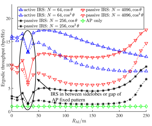
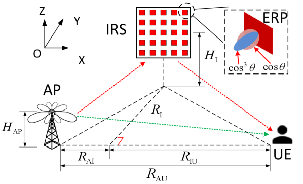
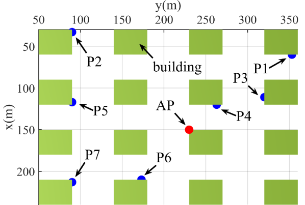
In order to analyze the link performance, we consider the scenario depicted in Fig. 2, with additional parameters given by $R_{\rm{AU}}=250$ m, $R_{\rm{I}}=10$ m and $H_{\rm{I}}=10$ m. The signals received by the UE have two types: direct signals from the AP and reflected signals from the IRS. We assum LoS links for AP-IRS and IRS-UE, and the NLoS link for AP-UE. Different ergodic throughput for the UE can be achieved when the IRS’s horizontal distance $R_{\rm{AI}}$ is changed. To draw a comparison, experiments were conducted with different number of IRS elements. Moreover, two ERPs for the IRS are considered, with $G_{\rm{i}}=$ 6 dBi (i.e. $\cos{\theta}$) and $G_{\rm{i}}=$ 9 dBi (i.e. $\cos^{3}{\theta}$), respectively. We also consider a baseline case without IRS. The simulation results are shown in Fig. 3.

It can be seen that deploying IRS (passive or active) brings significant performance improvement. Notice that when the $R_{\rm{AI}}=50$ m, the active IRS ($N=64$) outperforms the passive IRS ($N=256$) significantly, with the gap up to about 12bps/Hz. However, on the UE side, the performance of the active IRS ($N=64$) and the passive IRS ($N=256$) are close to each other. This is primarily due to the increased effect of active noise when the active IRS is close to the UE. Additionally, it has been observed that when the total number of passive IRS elements is increased, such as $N=4096$, its link performance improves significantly and can surpass the active IRS at some locations. Nonetheless, it should be noted that in practical implementations, a passive IRS with a large number of elements may lead to increased cost as well as challenges in channel estimation and beamforming. Moreover, the overall performance corresponding to the ERP of $\cos{\theta}$ is better than that of the ERP of $\cos^{3}{\theta}$. This is because the more focused antenna gain leads to diminished gain when the incident and departure angles deviate from the center of the beam. Furthermore, the fixed pattern of the AP impacts the link performance. When the signal falls into the sidelobes or gap of the AP’s fixed pattern, a noticeable degradation in performance can occur.

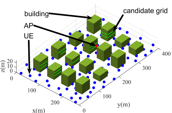
As shown in Fig. 4, we consider a scenario with $4\times 4=16$ buildings within an area of 270 m by 400 m. Each building has a length of 30 m and a width of 40 m. The building heights are randomly generated within a range of 12 to 22 meters. Additionally, 100 UEs or PoIs are randomly distributed on the streets, and there are 149 grid points available for IRS deployment.

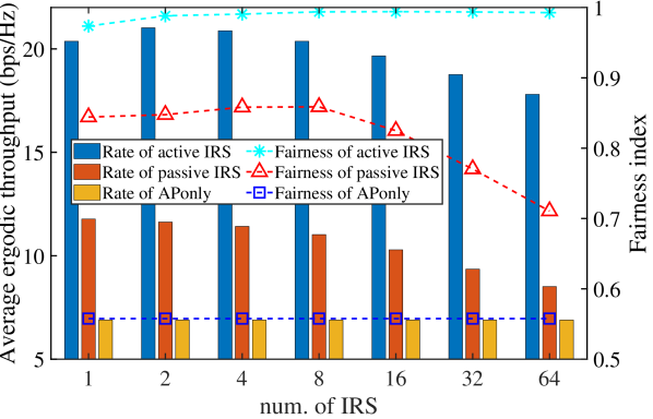
This section discusses the performance variation when a total number of elements are equally divided into different number of distributed IRSs. The experimental setup is similar to the previous section, with the same total number of elements $N=1024$ for both active and passive IRS. The results are shown in Fig. 5. It is found that to maximize average ergodic throughput, there exists a more suitable division for the active IRS. For example, in the considered setup here, it’s best to divide into 2 active IRSs. On the other hand, for the passive IRS, dividing it into more IRSs does not bring the expected benefits. This is because the more divisions there are, the smaller each IRS becomes, and the benefits that each UE receives from a single IRS become much smaller as well. Notice that, in terms of the fairness index²²2This index is defined as $J\triangleq\frac{(\sum_{u\in\mathcal{U}}R_{u})^{2}}{|\mathcal{U}|\sum_{u\in\mathcal{U}}R_{u}^{2}}$, where $J\in(0,1]$ and a higher $J$ represents better fairness., the fairness of active IRS is improved with more divisions, but the fairness of passive IRS is decreased with more divisions. This is because passive IRS is more suitable for deploying at the AP side or the UE side. When passive IRS is deployed at the UE side, it only serves the UEs in its vicinity, which results in a wider gap in the performance among the UEs.

To visualize the optimal deployment results, the dividing schemes with 1, 2, and 4 IRSs are plotted as shown in Fig. 6. The result indicates that when the total elements are divided into only one IRS, the optimal deployment location is relatively close to the APs for both the active and passive IRS. this is because it allows all the UEs to benefit from the IRS beamforming as much as possible, and maximizes the average ergodic throughput of all UEs. When divided into multiple IRSs, such as 4 IRSs, the optimal deployment locations for active and passive are different. For active IRSs, the IRSs can be placed farther away from the APs because the active IRSs have power amplification. However, for the passive IRSs, the optimal deployment location of the IRSs will not be very far away from the APs so as to increase the power reaching the IRSs.

In contrast to the preceding two subsections, the purpose of optimization here is to maximize the coverage ratio of the UEs. We substitute the objective function with the sum of coverage indicators in optimization problem (P1) and solve it using Gurobi. The main parameter settings are the same as the previous ones, while a larger area of 1080 m$\times$1600 m is considered. Moreover, the number of UEs is also expanded to 200, the length and width of each grid are 20 m and 7 m, and the number of selected candidate grid points is 176. Note that at longer distances, the coverage capability of the AP is weakened, and it is more meaningful to introduce the IRS for coverage enhancement.

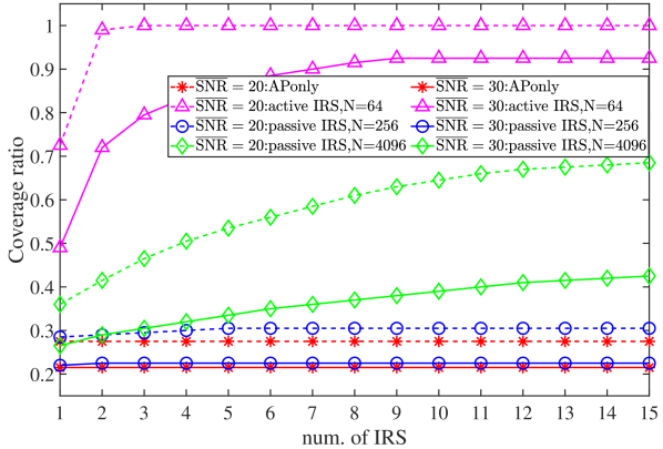
In this experiments, we set the SNR thresholds as $\overline{\rm{SNR}}=20\,\rm{dB},30\,\rm{dB}$, respectively. The experimental results are shown in Fig. 7. It is evident that the deployment of IRSs can enhance network coverage, irrespective of whether thresholds are set at 20 dB or 30 dB. However, active IRSs exhibit superior efficacy, achieving substantial coverage improvements with a smaller number of IRSs. In contrast, passive IRSs require a greater number and larger size to achieve comparable coverage enhancements. Especially at high thresholds (i.e., $\overline{\rm{SNR}}=30\,\rm{dB}$), the coverage performance improvement due to passive IRSs is more constrained. This limitation arises because passive IRSs have an inherently weaker channel enhancement capability, which is insufficient to meet the demand of a higher threshold.

References

- [1] Q. Wu and R. Zhang, “Towards smart and reconfigurable environment: Intelligent reflecting surface aided wireless network,” IEEE Communications Magazine, vol. 58, no. 1, pp. 106–112, 2019.
- [2] L. Dai, B. Wang, M. Wang, X. Yang, J. Tan, S. Bi, S. Xu, F. Yang, Z. Chen, M. Di Renzo et al., “Reconfigurable intelligent surface-based wireless communications: Antenna design, prototyping, and experimental results,” IEEE access, vol. 8, pp. 45 913–45 923, 2020.
- [3] S. Alfattani, W. Jaafar, Y. Hmamouche, H. Yanikomeroglu, and A. Yongaçoglu, “Link budget analysis for reconfigurable smart surfaces in aerial platforms,” IEEE Open Journal of the Communications Society, vol. 2, pp. 1980–1995, 2021.
- [4] Q. Wu and R. Zhang, “Intelligent reflecting surface enhanced wireless network: Joint active and passive beamforming design,” in 2018 IEEE Global Communications Conference (GLOBECOM). IEEE, 2018, pp. 1–6.
- [5] Q. Wu, S. Zhang, B. Zheng, C. You, and R. Zhang, “Intelligent reflecting surface-aided wireless communications: A tutorial,” IEEE Transactions on Communications, vol. 69, no. 5, pp. 3313–3351, 2021.
- [6] C. You and R. Zhang, “Wireless communication aided by intelligent reflecting surface: Active or passive?” IEEE Wireless Communications Letters, vol. 10, no. 12, pp. 2659–2663, 2021.
- [7] Z. Zhang, L. Dai, X. Chen, C. Liu, F. Yang, R. Schober, and H. V. Poor, “Active RIS vs. passive RIS: Which will prevail in 6G?” IEEE Transactions on Communications, vol. 71, no. 3, pp. 1707–1725, 2022.
- [8] W. Tang, X. Chen, M. Z. Chen, J. Y. Dai, Y. Han, M. Di Renzo, S. Jin, Q. Cheng, and T. J. Cui, “Path loss modeling and measurements for reconfigurable intelligent surfaces in the millimeter-wave frequency band,” IEEE Transactions on Communications, vol. 70, no. 9, pp. 6259–6276, 2022.
- [9] X. Chen, J. Lyu, and L. Fu, “IRS-aided sectorized base station design and 3D coverage performance analysis,” in 2023 IEEE/ACM 31st International Symposium on Quality of Service (IWQoS). IEEE, 2023, pp. 01–10.
- [10] S. Zhang and R. Zhang, “Intelligent reflecting surface aided multi-user communication: Capacity region and deployment strategy,” IEEE Transactions on Communications, vol. 69, no. 9, pp. 5790–5806, 2021.
- [11] B. Ling, J. Lyu, and L. Fu, “Placement optimization and power control in intelligent reflecting surface aided multiuser system,” in 2021 IEEE Global Communications Conference (GLOBECOM). IEEE, 2021, pp. 1–6.
- [12] M. Fu and R. Zhang, “Active and passive IRS jointly aided communication: Deployment design and achievable rate,” IEEE Wireless Communications Letters, vol. 12, no. 2, pp. 302–306, 2022.
- [13] Z. Kang, C. You, and R. Zhang, “Double-active-IRS aided wireless communication: Deployment optimization and capacity scaling,” IEEE Wireless Communications Letters, 2023.
- [14] W. Tang, M. Z. Chen, X. Chen, J. Y. Dai, Y. Han, M. Di Renzo, Y. Zeng, S. Jin, Q. Cheng, and T. J. Cui, “Wireless communications with reconfigurable intelligent surface: Path loss modeling and experimental measurement,” IEEE Transactions on Wireless Communications, vol. 20, no. 1, pp. 421–439, 2020.
- [15] J. Lyu and R. Zhang, “Network-connected UAV: 3-D system modeling and coverage performance analysis,” IEEE Internet of Things Journal, vol. 6, no. 4, pp. 7048–7060, 2019.
- [16] H. Yang, M. H. Herben, I. J. Akkermans, and P. F. Smulders, “Impact analysis of directional antennas and multiantenna beamformers on radio transmission,” IEEE transactions on vehicular technology, vol. 57, no. 3, pp. 1695–1707, 2008.
- [17] 3GPP TR36.777, “Study on enhanced LTE support for aerial vehicles,” V1.0.0.
- [18] 3GPP TR25.996, “Spatial channel model for multiple input multiple output (MIMO) simulations,” V16.0.0.
- [19] Gurobi Optimization Inc., “Gurobi Optimizer Reference Manual.” [Online]. Available: http://www.gurobi.com/documentation/