Campus E1.7, Saarland University, 66041 Saarbrücken, Germany.
{gierke,peter}@mia.uni-saarland.de
Skeletonisation Scale-Spaces
Abstract
The medial axis transform is a well-known tool for shape recognition. Instead of the object contour, it equivalently describes a binary object in terms of a skeleton containing all centres of maximal inscribed discs. While this shape descriptor is useful for many applications, it is also sensitive to noise: Small boundary perturbations can result in large unwanted expansions of the skeleton. Pruning offers a remedy by removing unwanted skeleton parts. In our contribution, we generalise this principle to skeleton sparsification: We show that subsequently removing parts of the skeleton simplifies the associated shape in a hierarchical manner that obeys scale-space properties. To this end, we provide both a continuous and discrete theory that incorporates architectural and simplification statements as well as invariances. We illustrate how our skeletonisation scale-spaces can be employed for practical applications with two proof-of-concept implementations for pruning and compression.
Keywords:
skeletonisation medial axis scale-space sparsification.1 Introduction
Classical scale-space theory is closely connected to shape analysis [24]: In particular, morphological scale-spaces [1, 5, 7, 9, 20, 28] consider the evolution of object boundaries under operations derived from dilation and erosion [25]. However, the silhouette is not the only way to describe a shape. Blum [4] has proposed the medial axis transform (MAT) as an equivalent shape descriptor motivated from the grass fire analogy: Propagating fronts originating from the object contour meet in the middle of the object, creating shocks. These locations define the skeleton of the shape, from which the full object can be reconstructed. Multi-scale ideas have also been explored for the MAT and related concepts with a primary focus on stability under noisy shape boundaries [18, 19].
Recently, Cárdenas et al. [6] have used image sparsification to define scale-spaces: They gradually remove image pixels and reconstruct the evolving image from this sparse data. This resembles skeleton pruning [23], which removes unwanted skeleton parts arising for instance from boundary noise. Leveraging this similarity, we establish novel connections between scale-space and MAT theory. Our goal is to generalise the concept of skeleton pruning in a formal scale-space setting by translating the sparsification paradigm from images to the medial axis.
Our Contributions. To this end, we propose a scale-space framework for shape evolutions that arise from sequential sparsification of skeletons. Inspired by the work of Cárdenas et al. [6], we describe the order in which skeleton points are removed in terms of a sparsification path. Based on a small amount of requirements, we establish architectural, simplification, and invariance properties for our scale-spaces. With a compression and a pruning example, we demonstrate how the sparsification path can be adapted to different practical applications. In particular, by imposing task-specific requirements on the sparsification path, we achieve additional theoretical guarantees for each application.
Related Work. Our scale-space theory relies on the axiomatic frameworks that were developed for classical scale-spaces based on partial differential equations (PDEs) [1, 8, 10, 21, 29], in particular on the work of Alvarez et al. [1]. For a comprehensive overview we refer to Weickert [29]. Due to their focus on shape analysis, morphological scale-spaces [1, 5, 7, 9, 20, 28] are conceptually closer to our approach. However, they analyse the evolution of the shape boundary, while we consider the medial axis to characterise shapes.
Deriving a scale-space from a shrinking skeleton is closely related to the sparsification scale-spaces of Cárdenas et al. [6], who remove image pixels successively instead of skeleton points and reconstruct with inpainting. For the medial axis, this can be seen as a form of pruning [3, 11, 13, 23, 22, 26]. Ogniewicz [13] proposed a scale-space-inspired hierarchic pruning similar to our branch pruning in Section 4. It is however practice-oriented, less general, and includes no systematic investigation of scale-space properties.
Besides the concept of hierarchy in pruning, connections between MAT and scale-space theory are rare. The multi-scale medial axis of Pizer et al. [16] consist of curves in scale-space representing middle points. Similarly, image cores [17] generalise the MAT based on scale-space theory to gain invariances. Tsogkas and Kokkinos [27] have used multi-scale concepts in a MAT-inspired learning approach to compute symmetry axes.
2 Review: Skeletonisation
For our skeletonisation scale-spaces, we require definitions of objects, distances, and the medial axis transform (MAT) [4]. We consider a binary image as a function that maps the image domain to the background value and the object value . The object is defined by set and denotes its boundary. We assume that is bounded and closed, such that its boundary belongs to the set. Hence, is a compact set. Furthermore, let denote the Euclidean distance for .
Definition 1 (Distance Map )
The distance map denotes the minimal distance to the boundary according to
| (1) |
The distance map allows us to define as the largest disc around that is fully contained in . With such inscribed discs we can define the medial axis.
Definition 2 (Skeleton )
The skeleton or medial axis (MA) is defined as the set of centres of inscribed discs of maximal radius:
In the definition, we call the disc around maximal, since it is not fully contained in any other larger disc around a skeleton point . Equivalently, is the set of skeleton points with at least two equidistant boundary points.
Definition 3 (Skeleton, Reconstruction, and Object Transform)
The skeleton transform maps the image to its skeleton . The reconstruction transform is defined via the object transform
| (2) |
Since is a continuous mapping of the compact set , all reconstructions are compact as well and . In addition to this continuous case, we also consider discrete images with resolution written as vectors with the discrete image domain . With the Euclidean distance between the pixel centres of and discrete discs, we transfer all other definitions from the continuous to the discrete setting. However, using discrete discs in Definition 3 can lead to and thus . We discuss the consequences of these observations for our scale-spaces in Section 3.1.
3 Skeletonisation Scale-Spaces
Inspired by the work of Cárdenas et al. [6], we define skeletonisation scale-spaces as the family of images emerging from successively removing parts of an initial skeleton. The order of this pruning is defined by sparsification paths.
Definition 4 (Sparsification Path)
Given a skeleton , a sparsification path with is an ordered collection of non-empty sets that form a partition of , i.e. for all : , , and .
In Section 4, we show that the sparsification path is a design tool for task-specific scale-spaces. Given the path, we can define the scale-space itself.
Definition 5 (Skeletonisation Scale-Space)
Consider the binary image with domain , skeleton , reconstruction and sparsification path partitioning , . The skeletonisation scale-space is the family of images and skeletons obeying
-
1.
,
-
2.
for ,
-
3.
and for .
At every scale , we obtain a skeleton-image-pair by successively removing from the skeleton according to the sparsification path and reconstruction from the pruned skeleton. We grant full flexibility regarding the choice of the sets and number of sparsification steps. It implies the discrete scales.
So far, our definition applies to space-continuous skeletons. Analogously, we define fully discrete skeletonisation scale-spaces: We replace the continuous image by its discrete counterpart with pixels and use the discrete definitions of skeletons and the associated transforms from Section 2. Then, all other definitions for sparsification path and scale-space carry over directly. In Section 3.1, we consider scale-space properties primarily for the continuous formulation. In case those properties do not apply to the discrete setting, we discuss these differences explicitly.
3.1 Generalised Scale-Space Properties
We investigate skeletonisation scale-spaces in the sense of Definition 5 from the perspective of scale-space research. Specifically, we show how properties established by Alvarez et al. [1] transfer to this new class of scale-space.
Property 1: (Original Skeleton as Initial State).
By Definition 5, at scale , the skeleton is the skeleton of the original object contained in the image . In the continuous setting, the image is thus the original image due to . For the discrete case, the reconstruction transform is only an approximation, not an inverse of and thus only holds.
Property 2: (Causality).
It does not matter if the sparsification path is traversed from the initial scale to scale or from any intermediate scale: The resulting skeleton-image-pair at scale remains the same. According to Definition 5, for and , we have
| (3) |
Thus, we can reach scale equivalently in steps from scale or in steps from scale . Since the skeleton at scale remains the same, this also holds for the image .
Property 3: (Lyapunov Sequences).
Lyapunov sequences quantify the simplification of the shape. In the following, we specify generic sequences that apply to all skeletonisation scale-spaces. In Section 4, we show that for specific tasks, we can find meaningful specialised Lyapunov sequences by imposing additional requirements.
Proposition 1 (Decreasing Object Area)
The area of the object decreases as the scale parameter increases, i.e. for .
Proof
For the path we have and thus
Therefore, we can derive
Thus, we can conclude . ∎
Similarly, we can also consider the spatial dimensions of the object. In the following, the diameter of a closed set is defined as
where is the continuous or discrete distance function. Then, the diameter of the reconstructed object defines a Lyapunov sequence.
Proposition 2 (Decreasing Object Diameter)
The object diameter decreases with increasing scale , i.e. for , we have
| (4) |
Proof
Assume that . Then, there are with . However, from the proof for Proposition 1, we know and hence also . This is a contradiction to the definition of the diameter and our assumption. Thus, the proposition holds. ∎
Property 4: (Invariance).
At each scale , the skeleton uniquely defines the skeleton-image-pair. Therefore, the scale-space inherits all invariances that apply to skeletons. This includes translations, rotations, scaling, and mirroring. For each such transformation we have .
In the discrete setting this holds only for on-grid transformations that preserve the shape. This includes on-grid translations, rotations, and mirroring along image axis.
4 Task-Specific Skeletonisation Scale-Spaces
So far, our generic scale-space framework only demands very few requirements. With the sparsification path from Definition 4, we can trade stricter requirements for application-specific scale-space properties. Just as sparsification scale-spaces [6], our framework allows uncommitted strategies that prune the skeleton without dependency on the input shape. However, committed approaches are often more interesting: They adapt to the evolving shape according to desirable properties for practical use. To illustrate this principle, we provide two examples of task-specific skeletonisation scale-spaces. We also show results for an implementation that uses the maximal disc thinning algorithm MDT [15] for skeleton computation. Therefore, we directly consider the discrete setting in the following.
4.1 Skeletonisation Scale-Spaces for Compression
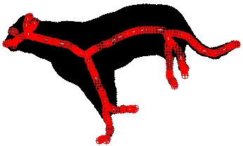
First, inspired by the work of Mühlhaus [12], we propose a MAT-based scale-space for shape compression. It reduces the amount of skeleton points to a very sparse subset while keeping the shape reconstruction as exact as possible. Since we are only interested in the scale-space aspect of such an application, we do not discuss actual coding here and refer to Mühlhaus [12] instead. Our goal is to remove points in ascending order of their influence on the reconstruction. To this end, we define the reconstruction impact of a given set as the part of the object that can only be reconstructed by its skeleton points.
Definition 6 (Reconstruction Impact)
For a set of skeleton points and we define the reconstruction impact by
| (5) |
Removing from the skeleton implies removing from the object, i.e.
| (6) |
Based on the reconstruction influence, Algorithm 1 defines a skeleton compression path that minimises the reconstruction error. For the sake of a convenient notation, we define for a given pixel index .
To demonstrate that this path indeed fulfils our compression goals, we consider the relative reconstruction error . This ratio of missing object points and total object points is a simplified scale-space version of the exactness of reconstruction criterion for skeleton quality [15]:
| (7) |
Note that this captures all possible reconstruction errors since removing skeleton points can only reduce the reconstructed area according to Proposition 1. Since is decreasing for coarser scales, the relative error increases and thus constitutes another Lyapunov sequence as a corollary to Proposition 1. Beyond that, we can also guarantee a minimal increase in error as desired for compression.
Proposition 3 (Minimal Relative Error Increase)
Among all possible sparsification paths, for all , the increase in relative error is minimal for a skeleton compression scale-space.
This holds directly since according to Eq. (6). By definition, Algorithm 1 selects such that is minimised over all possible choices of . Thus, a skeleton compression scale-space guarantees that at each scale we have a sparse skeleton with the smallest possible relative error.
Another quality measure for the discrete medial axis is skeleton minimality [15]. It relates the number of object points to the number of skeleton points needed to represent the object by
| (8) |
For compression purposes, skeleton minimality should be as small as possible, which implies that only a small amount of skeleton points needs to be stored to reconstruct a large object area. For our skeleton compression scale-space, this is reflected by a corresponding Lyapunov sequence.
Proposition 4 (Skeleton Minimality is a Lyapunov Sequence)
Skeleton minimality decreases with increasing scale , i.e. .
Proof
First, we decompose according to the sparsification path from Definition 5 and the reconstruction impact from Eq. (6). This yields
| (9) |
Furthermore, due to the sorting in Algorithm 1, the average unique area of the removed points in is smaller or equal to the average unique area of the remaining skeleton points in , i.e.
| (10) |
Combining both Eq. (9) and Eq. (10), we can show our claim by
| (11) | ||||||
| (12) |
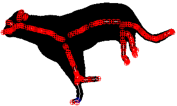
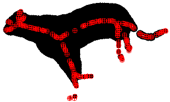
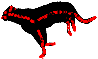
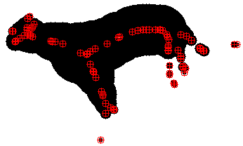
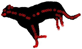
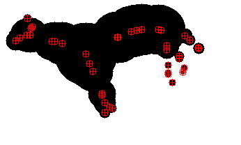
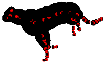
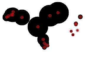
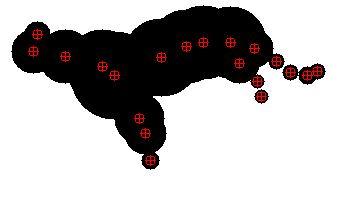
In Fig. 1, we compare our committed compression scale-space to an uncommitted scale-space where the sparsification path is chosen in a uniformly random order. While the evolution behaves similarly at fine scales, the reconstruction error is consistently lower for the compression path. At coarse scales, the compression path even yields error reduction and is thus indeed task-adaptive.
4.2 Skeletonisation Scale-Spaces for Branch Pruning
Pruning [3, 11, 13, 23, 22, 26] has different goals than compression. It is often performed as a preprocessing step for applications such as shape recognition and matching. Here, the connectivity and structure of the skeleton are essential while the amount of skeleton points and thus the coding cost is irrelevant.
Therefore, we design the sparsification path to preserve skeleton structure in two ways. First, our pruning has to be homotopy preserving, i.e. it should not disconnect the medial axis. Furthermore, we take into account semantically important end- and branching points of the skeleton. We can quantify their importance by using skeleton complexity [15] as a third quality measure.
To this end, we require two neighbourhood definitions. Let a 4-neighbourhood contain left, right, upper, and lower neighbours, while an 8-neighbourhood additionally contains the diagonal neighbours.
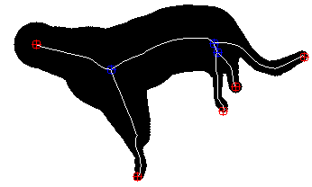
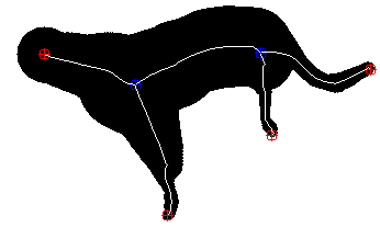
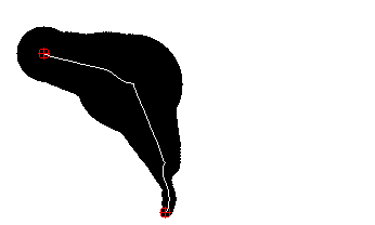
| original | segmentation | skeleton |
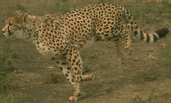 |
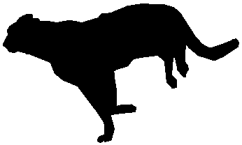 |
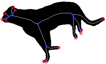 |
| random | compression | branch pruning |
 |
 |
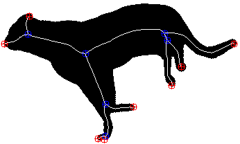 |
| SKEL 320, ERR 1397 | SKEL 320, ERR 1097 | SKEL 647, ERR 1174 |
 |
 |
 |
| SKEL 160, ERR 2051 | SKEL 160, ERR 1225 | SKEL 530, ERR 1931 |
 |
 |
 |
| SKEL 80, ERR 3347 | SKEL 80, ERR 1440 | SKEL 492, ERR 2302 |
 |
 |
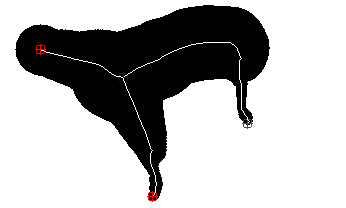 |
| SKEL 40, ERR 4378 | SKEL 40, ERR 2147 | SKEL 392, ERR 3603 |
 |
 |
 |
| SKEL 20, ERR 8918 | SKEL 20, ERR 3803 | SKEL 203, ERR 12156 |
Definition 7 (Endpoints, Branching Points, Simple Points, and Arcs)
-
•
An endpoint of has either: 1.) zero or one skeleton points in their 8-neighbourhood; 2.) two skeleton points in its 8-neighbourhood which are adjacent to one another; 3.) three skeleton points in its 8-neighbourhood that are either all above, below, left, or right of . We denote the set of endpoints by .
-
•
A branching point of has at least three skeleton points in its 8-neighbourhood which are not horizontally or vertically adjacent. We denote the set of branching points by .
-
•
A simple point is a skeleton point which is neither an endpoint nor a branching point. We write .
-
•
We define as the set of all arcs/branches. Each of its elements fulfils two properties: 1.) The arc is connected, i.e. for each the points and share an 8-neighbourhood. 2.) Exactly and are end- or branching points, the rest of the are simple.
Endpoints and branching points are much more important for shape recognition than simple points. They mark where individual arcs of the skeleton intersect or end. Thereby, they characterise the shape together with the arc lengths. Therefore, skeleton complexity considers the number of important points as
| (13) |
Spurious branches resulting from noise increase this measure significantly due to added end- and branching points. Note that typically, such a change has marginal impact on the relative error, while skeleton minimality rises based on the added arc length. With these definitions and the combined goals of preserving homotopy while not increasing skeleton complexity, we define the branch pruning path in Algorithm 2. The simple rule of only removing full skeleton branches with endpoints achieves our goals. A skeleton can only be disconnected if branching or simple points are removed. We can show that complexity is decreasing for coarser scales and thus constitutes a Lyapunov sequence for the pruning scale-space.
Proposition 5 (Skeleton Complexity is a Lyapunov Sequence)
Skeleton complexity decreases with increasing scale , i.e. .
Proof
For a scale , there are the following possible cases for the next step in the sparsification path:
- Case 1:
-
has exactly two endpoints, which are both removed. The branch is not connected to other skeleton components and thus cannot influence other points. Then .
- Case 2:
-
By Algorithm 2, has exactly one endpoint, which is removed. The arc is connected to a branching point. Its role can change to an end or simple point, but this cannot increase complexity. Thus, .
- Case 3:
-
. The remaining skeleton is removed, thus . ∎
In Fig. 1, branch pruning differs significantly from uncommitted random and compression scale-spaces. Note that visualising a meaningful evolution requires different scales than the other paths. Throughout the evolution, the branch pruning gradually reduces complexity: The joint number of end- and branching points decreases as desired. Homotopy is also preserved while the reconstruction error is kept as low as possible under these constraints. However, preserving the structure also comes at a cost. With an order of magnitude less points, the compression path yields only a quarter of the reconstruction error. On the flips-side, it sacrifices homotopy and creates many new end points.
5 Conclusions and Outlook
With skeletonisation scale-spaces, we provide a new hierarchical perspective on shape analysis. They combine the principles of the medial axis transform [4] with sparsification scale-space paradigms [6, 14]. Our scale-space framework allows adaptions to different applications via committed sparsification paths. In particular, our compression and branch pruning examples demonstrate that suitable requirements result in theoretical guarantees for reconstruction quality or skeleton structure in terms of Lyapunov sequences.
In the future, we plan to investigate connections between the skeleton evolution and the implied boundary evolution. Moreover, extending our theory to the fully continuous setting could yield new insights. Finally, we would like to explore full-fledged compression or shape matching approaches based on scale-spaces.
References
- [1] Alvarez, L., Guichard, F., Lions, P.L., Morel, J.M.: Axioms and fundamental equations in image processing. Archive for Rational Mechanics and Analysis 123, 199–257 (Sep 1993)
- [2] Arbelaez, P., Maire, M., Fowlkes, C., Malik, J.: Contour detection and hierarchical image segmentation. IEEE Transactions on Pattern Analysis and Machine Intelligence 33(5), 898–916 (Aug 2011)
- [3] Bai, X., Latecki, L.J., Liu, W.Y.: Skeleton pruning by contour partitioning with discrete curve evolution. IEEE Transactions on Pattern Analysis and Machine Intelligence 29(3), 449–462 (Jan 2007)
- [4] Blum, H.: A transformation for extracting new descriptors of shape. In: Wathen-Dunn, W. (ed.) Models for the Perception of Speech and Visual Form, pp. 362–380. MIT press, Cambridge, MA (1967)
- [5] Brockett, R.W., Maragos, P.: Evolution equations for continuous-scale morphology. In: Proc. 1992 IEEE International Conference on Acoustics, Speech and Signal Processing. vol. 3, pp. 125–128. San Francisco, CA (Mar 1992)
- [6] Cárdenas, M., Peter, P., Weickert, J.: Sparsification scale-spaces. In: Lellmann, J., Burger, M., Modersitzki, J. (eds.) Scale Space and Variational Methods in Computer Vision, Lecture Notes in Computer Science, vol. 11603, pp. 303–314. Springer, Cham (2019)
- [7] Caselles, V., Sbert, C.: What is the best causal scale space for three-dimensional images? SIAM Journal on Applied Mathematics 56(4), 1199–1246 (1996)
- [8] Iijima, T.: Basic theory on normalization of pattern (in case of typical one-dimensional pattern). Bulletin of the Electrotechnical Laboratory 26, 368–388 (Jan 1962), in Japanese
- [9] Kimia, B.B., Siddiqi, K.: Geometric heat equation and non-linear diffusion of shapes and images. Computer Vision and Image Understanding 64, 305–322 (1996)
- [10] Lindeberg, T.: Generalized Gaussian scale-space axiomatics comprising linear scale-space, affine scale-space and spatio-temporal scale-space. Journal of Mathematical Imaging and Vision 40, 36–81 (2011)
- [11] Montero, A.S., Lang, J.: Skeleton pruning by contour approximation and the integer medial axis transform. Computers & Graphics 36(5), 477–487 (Mar 2012)
- [12] Mühlhaus, M.: Compressing Binary Images with the Medial Axis Transform. Bachelor’s thesis, Faculty of Mathematics and Computer Science, Saarland University (2020)
- [13] Ogniewicz, R.L.: Automatic medial axis pruning based on characteristics of the skeleton-space. In: Shape, Structure and Pattern Recognition – Proc. 1994 IAPR International Workshop. pp. 23–32. Nahariya, Israel (Oct 1994)
- [14] Peter, P.: Quantisation scale-spaces. In: Elmoataz, A., Fadili, J., Quéau, Y., Rabin, J., Simon, L. (eds.) Scale Space and Variational Methods in Computer Vision, Lecture Notes in Computer Science, vol. 12679, pp. 15–26. Springer, Cham (2021)
- [15] Peter, P., Breuß, M.: Refined homotopic thinning algorithms and quality measures for skeletonisation methods. In: Breuß, M., Bruckstein, A., Maragos, P. (eds.) Innovations for Shape Analysis: Models and Algorithms, pp. 77–92. Mathematics and Visualization, Springer, Berlin (2013)
- [16] Pizer, S.M., Burbeck, C.A., Coggins, J.M., Fritsch, D.S., Morse, B.S.: Object shape before boundary shape: Scale-space medial axes. Journal of Mathematical Imaging and Vision 4(3), 303–313 (Jul 1994)
- [17] Pizer, S.M., Eberly, D., Fritsch, D.S., Morse, B.S.: Zoom-invariant vision of figural shape: The mathematics of cores. Computer Vision and Image Understanding 69(1), 55–71 (Jan 1998)
- [18] Pizer, S.M., Siddiqi, K., Székely, G., Damon, J.N., Zucker, S.W.: Multiscale medial loci and their properties. International Journal of Computer Vision 55, 155–179 (Nov 2003)
- [19] Saha, P.K., Borgefors, G., Sanniti di Baja, G.: A survey on skeletonization algorithms and their applications. Pattern Recognition Letters 76(C), 3––12 (Jun 2016)
- [20] Sapiro, G., Tannenbaum, A.: Affine invariant scale-space. International Journal of Computer Vision 11, 25–44 (1993)
- [21] Scherzer, O., Weickert, J.: Relations between regularization and diffusion filtering. Journal of Mathematical Imaging and Vision 12(1), 43–63 (Feb 2000)
- [22] Serino, L., Sanniti di Baja, G.: A new strategy for skeleton pruning. Pattern Recognition Letters 76, 41–48 (Jun 2016)
- [23] Shaked, D., Bruckstein, A.: Pruning medial axes. Computer Vision and Image Understanding 69(2), 156–169 (Feb 1998)
- [24] Siddiqi, K., Pizer, S.: Medial representations: mathematics, algorithms and applications, Computational Imaging and Vision, vol. 37. Springer, Dordrecht (2008)
- [25] Soille, P.: Morphological Image Analysis. Springer, Berlin, second edn. (2003)
- [26] Tam, R., Heidrich, W.: Feature-preserving medial axis noise removal. In: Proc. 7th European Conference on Computer Vision (ECCV), Part II. pp. 672–686. Copenhagen, Denmark (May 2002)
- [27] Tsogkas, S., Kokkinos, I.: Learning-based symmetry detection in natural images. In: Fitzgibbon, A., Lazebnik, S., Perona, P., Saito, Y., Schmid, C. (eds.) Computer Vision – ECCV 2012, Lecture Notes in Computer Science, vol. 7574, pp. 41–54. Spinger, Berlin (2012)
- [28] van den Boomgaard, R., Smeulders, A.: The morphological structure of images: The differential equations of morphological scale-space. IEEE Transactions on Pattern Analysis and Machine Intelligence 16, 1101–1113 (1994)
- [29] Weickert, J.: Anisotropic Diffusion in Image Processing. Teubner, Stuttgart (1998)