Skewed Bernstein–von Mises theorem
and skew–modal approximations

Daniele Durantelabel=e1 [ mark]daniele.durante@unibocconi.it Francesco Pozzalabel=e2 [ mark]francesco.pozza2@unibocconi.it Botond Szabolabel=e3 [ mark]botond.szabo@unibocconi.it Department of Decision Sciences and Institute for Data Science and Analytics, Bocconi University,
Institute for Data Science and Analytics, Bocconi University,

Abstract

Gaussian deterministic approximations are routinely employed in Bayesian statistics to ease inference when the target posterior of direct interest is intractable. Although these approximations are justified, in asymptotic regimes, by Bernstein–von Mises type results, in practice the expected Gaussian behavior may poorly represent the actual shape of the target posterior, thereby affecting approximation accuracy. Motivated by these considerations, we derive an improved class of closed–form and valid deterministic approximations of posterior distributions which arise from a novel treatment of a third–order version of the Laplace method yielding approximations within a tractable family of skew–symmetric distributions. Under general assumptions which also account for misspecified models and non–i.i.d. settings, this novel family of approximations is shown to have a total variation distance from the target posterior whose rate of convergence improves by at least one order of magnitude the one achieved by the Gaussian from the classical Bernstein–von Mises theorem. Specializing such a general result to the case of regular parametric models shows that the same improvement in approximation accuracy can be also established for polynomially bounded posterior functionals, including moments. Unlike other higher–order approximations based on, e.g., Edgeworth expansions, our results prove that it is possible to derive closed–form and valid densities which are expected to provide, in practice, a more accurate, yet similarly–tractable, alternative to Gaussian approximations of the target posterior of direct interest, while inheriting its limiting frequentist properties. We strengthen these arguments by developing a practical skew–modal approximation for both joint and marginal posteriors which achieves the same theoretical guarantees of its theoretical counterpart by replacing the unknown model parameters with the corresponding maximum a posteriori estimate. Simulation studies and real–data applications confirm that our theoretical results closely match the remarkable empirical performance observed in practice, even in finite, possibly small, sample regimes.

62F15,

62F03,

62E17,

Bernstein–von Mises theorem,

Deterministic approximation,

Skew–symmetric distribution,

keywords:

[class=MSC2020]

keywords:

\changefontsizes

14pt \startlocaldefs \endlocaldefs

, and

t1Co–funded by the European Union (ERC, BigBayesUQ, project number: 101041064). Views and opinions expressed are however those of the author(s) only and do not necessarily reflect those of the European Union or the European Research Council. Neither the European Union nor the granting authority can be held responsible for them.

t2Funded by the European Union (ERC, PrSc-HDBayLe, project number: 101076564). Views and opinions expressed are however those of the author(s) only and do not necessarily reflect those of the European Union or the European Research Council. Neither the European Union nor the granting authority can be held responsible for them.

1 Introduction

Modern Bayesian statistics relies extensively on deterministic approximations to facilitate inference in those challenging, yet routine, situations when the target posterior of direct interest is intractable (e.g., Tierney and Kadane, 1986; Minka, 2001; Rue, Martino and Chopin, 2009; Blei, Kucukelbir and McAuliffe, 2017). A natural option to enforce the desired tractability is to constrain the approximating distribution within a suitable family which facilitates the evaluation of functionals of interest for inference. To this end, both classical solutions, such as the approximation of posterior distributions induced by the Laplace method (e.g., Bishop, 2006, Ch. 4.4), and state–of–the–art strategies, including, for example, Gaussian variational Bayes (Opper and Archambeau, 2009) and standard implementations of expectation–propagation (Minka, 2001), employ Gaussian approximations. These further appear, either as the final solution or as a recurring building–block, also within several routinely–implemented alternatives, such as mean–field variational Bayes (Blei, Kucukelbir and McAuliffe, 2017) and integrated nested Laplace approximation (inla) (Rue, Martino and Chopin, 2009). See also Wang and Blei (2013), Chopin and Ridgway (2017), Durante and Rigon (2019), Ray and Szabó (2022) and Vehtari et al. (2020), among others, for further examples illustrating the relevance of Gaussian approximations.

From a theoretical perspective, the choice of the Gaussian family to approximate the posterior distribution is justified, in asymptotic regimes, by Bernstein–von Mises type results. In its classical formulation (Laplace, 1810; Bernstein, 1917; Von Mises, 1931; Le Cam, 1953; Le Cam and Yang, 1990; Van der Vaart, 2000), the Bernstein–von Mises theorem states that, in sufficiently regular parametric models, the posterior distribution converges in total variation (tv) distance, with probability tending to one under the law of the data, to a Gaussian distribution. The mean of such a limiting Gaussian is a known function of the true data–generative parameter, or any efficient estimator of this quantity, such as the maximum likelihood estimator, while the variance is the inverse of the Fisher information. Extensions of the Bernstein–von Mises theorem to more complex settings have also been made in recent years. Relevant contributions along these directions include, among others, generalizations to high-dimensional regimes (Boucheron and Gassiat, 2009; Spokoiny and Panov, 2021), along with in–depth treatments of misspecified (Kleijn and van der Vaart, 2012) and irregular (Bochkina and Green, 2014) models. Semiparametric settings have also been addressed (Bickel and Kleijn, 2012; Castillo and Rousseau, 2015). In the nonparametric context, Bernstein–von Mises type results do not hold in general, but the asymptotic Gaussianity can be still proved for weak Sobolev spaces via a multiscale analysis (Castillo and Nickl, 2014).

Besides providing crucial advances in the understanding of the limiting frequentist properties of posterior distributions, the above Bernstein–von Mises type results have also substantial implications in the design and in the theoretical justification of practical Gaussian deterministic approximations for intractable posterior distributions from, e.g., the Laplace method (Kasprzak, Giordano and Broderick, 2022), variational Bayes (vb) (Wang and Blei, 2019) and expectation–propagation (ep) (Dehaene and Barthelmé, 2018). Such a direction has led to important results. Nonetheless, in practical situations the Gaussian approximation may lack the required flexibility to closely match the actual shape of the posterior distribution of direct interest, thereby undermining accuracy when inference is based on such an approximation. In fact, as illustrated via two representative real–data clinical applications in Sections 5.2–5.3, the error in posterior mean estimation of the Gaussian approximation supported by the classical Bernstein–von Mises theorem is non–negligible not only in a study with low sample size $n=27$ and $d=3$ parameters, but also in a higher–dimensional application with $n=333$ and $d\approx n/2.5$ . Both regimes often occur in routine implementations. The results in Sections 5.2–5.3 further clarify that the issues encountered by the Gaussian approximation are mainly due to the inability of capturing the non–negligible skewness often displayed by the actual posterior in these settings. Such an asymmetric shape is inherent to routinely–studied posterior distributions. For example, Durante (2019), Fasano and Durante (2022) and Anceschi et al. (2023) have recently proved that, under a broad class of priors which includes multivariate normals, the posterior distribution induced by probit, multinomial probit and tobit models belongs to a skewed generalization of the Gaussian distribution known as unified skew–normal (sun) (Arellano-Valle and Azzalini, 2006). More generally, available extensions of Gaussian deterministic approximations which account, either explicitly or implicitly, for skewness (see e.g., Rue, Martino and Chopin, 2009; Challis and Barber, 2012; Fasano, Durante and Zanella, 2022) have shown evidence of improved empirical accuracy relative to their Gaussian counterparts. Nonetheless, these approximations are often model–specific and general justifications relying on Bernstein–von Mises type results are not available yet. In fact, in–depth theory and methods for skewed approximations are either lacking or are tailored to specific models and priors (Fasano, Durante and Zanella, 2022).

In this article, we cover the aforementioned gaps by deriving an improved class of closed–form, valid and theoretically–supported skewed approximations of generic posterior distributions. Such a class arises from a novel treatment of a higher–order version of the Laplace method which replaces the third–order term with a suitable univariate cumulative distribution function (cdf) satisfying mild regularity conditions. As clarified in Section 2.1, this new perspective yields tractable approximations that crucially belong to the broad and known skew–symmetric family (see e.g., Ma and Genton, 2004). More specifically, these approximations can be readily obtained by direct perturbation of the density of a multivariate Gaussian via a suitably–defined univariate cdf evaluated at a cubic function of the parameter. This implies that the proposed class of approximations admits straightforward i.i.d. sampling schemes facilitating direct Monte Carlo evaluation of any functional of interest for posterior inference. These are crucial advancements relative to other higher–order studies relying on Edgeworth or other types of representations (see e.g., Johnson, 1970; Weng, 2010; Kolassa and Kuffner, 2020, and references therein), which consider arbitrarily truncated versions of infinite expansions that do not necessarily correspond to closed–form valid densities, even after normalization — e.g., the density approximation is not guaranteed to be non–negative (e.g., Kolassa and Kuffner, 2020, Remark 11). This undermines the methodological and practical impact of current higher–order results which still fail to provide a natural, valid and general alternative to Gaussian deterministic approximations that can be readily employed in practice. In contrast, our novel results prove that a previously–unexplored treatment of specific higher–order expansions can actually yield valid, practical and theoretically–supported approximations, thereby opening the avenues to extend such a perspective to orders even higher than the third one; see also our final discussion in Section 6.

Section 2.2 clarifies that the proposed class of skew–symmetric approximations has also strong theoretical support in terms of accuracy improvements relative to its Gaussian counterpart. More specifically, in Theorem 2.1 we prove that the newly–proposed class of skew–symmetric approximations has a total variation distance from the target posterior distribution whose rate of convergence improves by at least one order of magnitude the one attained by the Gaussian from the classical Bernstein–von Mises theorem. Crucially, this result is derived under general assumptions which account for both misspecified models and non–i.i.d. settings. This yields an important refinement of standard Bernstein–von Mises type results clarifying that it is possible to derive closed–form and valid densities which are expected to provide, in practice, a more accurate, yet similarly–tractable, alternative to Gaussian approximations of the target posterior of direct interest, while inheriting its limiting frequentist properties. In Section 2.3 these general results are further specialized to, possibly non–i.i.d. and misspecified, regular parametric models, where $n\to\infty$ and the dimension $d$ of the parametric space is fixed. Under such a practically–relevant setting, we show that the proposed skew–symmetric approximation can be explicitly derived as a function of the log–prior and log–likelihood derivatives. Moreover, we prove that by replacing the classical Gaussian approximation from the Bernstein–von Mises theorem with such a newly–derived alternative yields a remarkable improvement in the rates of order $\sqrt{n}$ , up to a poly–log term. This gain is shown to hold not only for the tv distance from the target posterior, but also for the error in approximating polynomially bounded posterior functionals (e.g., moments).

The methodological impact of the theory in Section 2 is further strengthened in Section 4 through the development of a readily–applicable plug–in version for the proposed class of skew–symmetric approximations derived in Section 2.1. This is obtained by replacing the unknown true data–generating parameter in the theoretical construction with the corresponding maximum a posteriori estimate, or any other efficient estimator. The resulting solution is named skew–modal approximation and, under mild conditions, is shown to achieve the same improved rates of its theoretical counterpart, both in terms of the tv distance from the target posterior distribution and with respect to the approximation error for polynomially bounded posterior functionals. In such a practically–relevant setting, we further refine the theoretical analysis through the derivation of non–asymptotic bounds for the tv distance among the skew–modal approximation and the target posterior. These bounds are guaranteed to vanish also when the dimension $d$ grows with $n$ , as long as $d\ll n^{1/3}$ up to a poly–log term. Interestingly, this condition is related to those required either for $d$ (see e.g., Panov and Spokoiny, 2015) or for the notion of effective dimension $\tilde{d}$ (see Spokoiny and Panov, 2021; Spokoiny, 2023) in recent high–dimensional studies of the Gaussian Laplace approximation. However, unlike these studies, the bounds we derive vanish with $n$ , up to a poly–log term, rather than $\sqrt{n}$ , for any given dimensions. These advancements enable also the derivation of a novel lower bound for the tv distance among the Gaussian Laplace approximation and the target posterior, which is shown to still vanish with $\sqrt{n}$ . This result strengthens the proposed skew–modal solution whose associated upper bound vanishes with $n$ , up to a poly–log term. When the focus of inference is not on the joint posterior but rather on its marginals, we further derive in Section 4.2 accurate skew–modal approximations for such marginals that inherit the same theory guarantees while scaling up computation.

The superior empirical performance of the newly–proposed class of skew–symmetric approximations and the practical consequences of our theoretical results on the improved rates are illustrated through both simulation studies and two real–data applications in Sections 3 and 5. All these numerical analyses demonstrate that the remarkable theoretical improvements encoded within the rates we derive closely match the empirical behavior observed in practice even in finite, possibly small, sample regimes. This translates into noticeable empirical accuracy gains relative to the classical Gaussian–modal approximation from the Laplace method. Even more, in the real–data application the proposed skew–modal approximation also displays a highly competitive performance with respect to more sophisticated state–of–the–art Gaussian and non–Gaussian approximations from mean–field vb and expectation–propagation (ep) (Minka, 2001; Blei, Kucukelbir and McAuliffe, 2017; Chopin and Ridgway, 2017; Durante and Rigon, 2019; Fasano, Durante and Zanella, 2022).

As discussed in the concluding remarks in Section 6, the above results stimulate future advancements aimed at refining the accuracy of other Gaussian approximations from, e.g., vb and ep, via the inclusion of skewness. To this end, our contribution provides the foundations to achieve this goal, and suggests that a natural and tractable class where to seek these improved approximations would be still the skew–symmetric family. Extensions to higher–order expansions beyond the third term are also discussed as directions of future research. Finally, notice that although the non–asymptotic bounds we derive for the skew–modal approximation in Section 4 yield refined theoretical results that can be readily proved for the general skew–symmetric class in Section 2, the practical consequences of non–asymptotic bounds and the associated constants is an ongoing area of research even for basic Gaussian approximations (see e.g., Kasprzak, Giordano and Broderick, 2022, and references therein). In this sense, it shall be emphasized that, in our case, even the asymptotic theoretical support encoded in the rates we derive finds empirical evidence in the finite–sample studies considered in Sections 3 and 5.

1.1 Notation

We denote with $\{X_{i}\}_{i=1}^{n}$ , $n\in\mathbbm{N}$ , a sequence of random variables with unknown true distribution $P_{0}^{n}$ . Moreover, let $\mathcal{P}_{\Theta}=\left\{P_{\theta}^{n},\theta\in\Theta\right\}$ , with $\Theta\subseteq\mathbb{R}^{d}$ , be a parametric family of distributions. In the following, we assume that there exists a common $\sigma$ –finite measure $\mu^{n}$ which dominates $P_{0}^{n}$ as well as all measures $P_{\theta}^{n}$ , and we denote by $p_{0}^{n}$ and $p_{\theta}^{n}$ the corresponding density functions. The Kullback–Leibler projection $P_{\theta_{*}}^{n}$ of $P_{0}^{n}$ on $\mathcal{P}_{\Theta}$ is defined as $P_{\theta_{*}}^{n}=\mbox{argmin}_{P_{\theta}^{n}\in\mathcal{P}_{\Theta}}\textsc{kl}(P_{0}^{n}\|P_{\theta}^{n})$ where $\textsc{kl}(P_{0}^{n}\|P_{\theta}^{n})$ denotes the Kullback–Leibler divergence between $P_{0}^{n}$ and $P_{\theta}^{n}$ . The log–likelihood of the, possibly misspecified, model is $\ell(\theta)=\ell(\theta,X^{n})=\log p_{\theta}^{n}\left(X^{n}\right)$ . Prior and posterior distributions are denoted by $\Pi(\cdot)$ and $\Pi_{n}(\cdot)$ , whereas the corresponding densities are indicated with $\pi(\cdot)$ and $\pi_{n}(\cdot)$ , respectively.

As mentioned in Section 1, our results rely on higher–order expansions and derivatives. To this end, we characterize operations among vectors, matrices and arrays in a compact manner by adopting the index notation along with the Einstein’s summation convention (see e.g., Pace and Salvan, 1997, p. 335). More specifically, the inner product $Z^{\intercal}a$ between the generic random vector $Z\in\mathbb{R}^{d},$ with components $Z_{s}$ for $s=1,\dots,d$ , and the vector of coefficients $a\in\mathbb{R}^{d}$ having elements $a_{s}$ for $s=1,\dots,d,$ is expressed as $a_{s}Z_{s}$ , with the sum being implicit in the repetition of the indexes. Similarly, if $B$ is a $d\times d$ matrix with entries $b_{st}$ for $s,t=1,\dots,d,$ the quadratic form $Z^{\intercal}BZ$ is expressed as $b_{st}Z_{s}Z_{t}.$ The generalization to operations involving arrays with higher dimensions is obtained under the same reasoning.

Leveraging the above notation, the score vector evaluated at $\theta_{*}$ is defined as

\displaystyle\ell^{(1)}_{\theta_{*}}=[\ell^{(1)}_{s}(\theta)]_{\mid\theta=\theta_{*}}\,=\,\left[(\partial/\partial\theta_{s})\ell(\theta)\right]_{\mid\theta=\theta_{*}}\in\mathbb{R}^{d},

whereas, the second, third and fourth order derivatives of $\ell(\theta)$ , still evaluated at $\theta_{*}$ , are

\displaystyle\begin{split}&\ell^{(2)}_{\theta_{*}}=[\ell^{(2)}_{st}(\theta)]_{\mid\theta=\theta_{*}}\,\,=\,[\partial/(\partial\theta_{s}\partial\theta_{t})\ell(\theta)]_{\mid\theta=\theta_{*}}\in\mathbb{R}^{d\times d},\\ &\ell^{(3)}_{\theta_{*}}=[\ell^{(3)}_{stl}(\theta)]_{\mid\theta=\theta_{*}}\,\,=\,[\partial/(\partial\theta_{s}\partial\theta_{t}\partial\theta_{l})\ell(\theta)]_{\mid\theta=\theta_{*}}\in\mathbb{R}^{d\times d\times d},\\ &\ell^{(4)}_{\theta_{*}}=[\ell^{(4)}_{stlk}(\theta)]_{\mid\theta=\theta_{*}}\,=\,[\partial/(\partial\theta_{s}\partial\theta_{t}\partial\theta_{l}\partial\theta_{k})\ell(\theta)]_{\mid\theta=\theta_{*}}\in\mathbb{R}^{d\times d\times d\times d},\end{split}

where all the indexes in the above definitions and in the subsequent ones go from $1$ to $d$ . The observed and expected Fisher information are denoted by $J_{\theta_{*}}=[j_{st}]=-[\ell^{(2)}_{\theta_{*},st}]\in\mathbb{R}^{d\times d}$ and $I_{\theta_{*}}=[i_{st}]=[\mathbb{E}_{0}^{n}j_{st}]\in\mathbb{R}^{d\times d}$ , respectively, where $\mathbb{E}_{0}^{n}$ is the expectation with respect to $P_{0}^{n}$ . In addition,

\displaystyle\begin{aligned} \log\pi^{(1)}_{\theta_{*}}=&[\log\pi(\theta)_{s}^{(1)}]_{\mid\theta=\theta_{*}}=\,[\partial/(\partial\theta_{s})\log\pi(\theta)]_{\mid\theta=\theta_{*}}\in\mathbb{R}^{d},\\ \log\pi^{(2)}_{\theta_{*}}=&[\log\pi(\theta)_{st}^{(2)}]_{\mid\theta=\theta_{*}}=\,[\partial/(\partial\theta_{s}\partial\theta_{t})\log\pi(\theta)]_{\mid\theta=\theta_{*}}\in\mathbb{R}^{d\times d},\\ \end{aligned}

represent the first two derivatives of the log–prior density, evaluated at $\theta_{*}.$

The Euclidean norm of a vector $a\in\mathbb{R}^{d}$ is denoted by $\|a\|$ , whereas, for a generic $d\times d$ matrix $B$ , the notation $|B|$ indicates its determinant, while $\lambda_{\textsc{min}}(B)$ and $\lambda_{\textsc{max}}(B)$ its minimum and maximum eigenvalue, respectively. Furthermore, $u\wedge v$ and $u\vee v$ correspond to $\min\{u,v\}$ and $\max\{u,v\}$ . For two positive sequences $u_{n},v_{n}$ we employ $u_{n}\lesssim v_{n}$ if there exists a universal positive constant $C$ such that $u_{n}\leq Cv_{n}$ . When $u_{n}\lesssim v_{n}$ and $v_{n}\lesssim u_{n}$ are satisfied simultaneously, we write $u_{n}\asymp v_{n}$ .

2 A skewed Bernstein–von Mises theorem

This section presents our first important contribution. In particular, Section 2.1 shows that, for Bayesian models satisfying a refined version of the local asymptotic normality (lan) condition (see e.g., Van der Vaart, 2000; Kleijn and van der Vaart, 2012), a previously–unexplored treatment of a third–order version of the Laplace method can yield a novel, closed–form and valid approximation of the posterior distribution. Crucially, this approximation is further shown to belong to the tractable skew–symmetric (sks) family (e.g., Ma and Genton, 2004). Focusing on this newly–derived class of sks approximations, we then prove in Section 2.2 that the $n$ –indexed sequence of tv distances between such a class and the target posterior has a rate which improves by at least one order of magnitude the one achieved under the classical Bernstein–von Mises theorem based on Gaussian approximations. Such a skewed Bernstein–von Mises type result is proved under general assumptions which account for misspecified models in non–i.i.d. settings. Section 2.3 then specializes this result to the practically–relevant context of regular parametric models with $n\to\infty$ and fixed $d$ . In this setting we prove that the improvement in rates over the Bernstein–von Mises theorem is by a multiplicative factor of order $\sqrt{n}$ , up to a poly–log term. This result is shown to hold not only for the tv distance from the posterior, but also for the error in approximating polynomially bounded posterior functionals.

Let $\delta_{n}\to 0$ be a generic norming rate governing the posterior contraction toward $\theta_{*}$ . Consistent with standard Bernstein–von Mises type theory (see e.g., Van der Vaart, 2000; Kleijn and van der Vaart, 2012), consider the re–parametrization $h=\delta_{n}^{-1}(\theta-\theta_{*})\in\mathbb{R}^{d}$ . Moreover, let $F(\cdot)\,:\,\mathbb{R}\to[0{,}1]$ denote any univariate cumulative distribution function which satisfies $F(-x)=1-F(x)$ and $F(x)\ {=}1/2+\eta x+O(x^{2}),\,x\to 0$ , for some $\eta\in\mathbb{R}$ . Then, the class of sks approximating densities $p_{\textsc{sks}}^{n}(h)$ we derive and study has the general form

\displaystyle p_{\textsc{sks}}^{n}(h)\,=\,2\phi_{d}\left(h;\xi,\Omega\right)w(h-\xi)=\,2\phi_{d}\left(h;\xi,\Omega\right)F(\alpha_{\eta}(h-\xi)),

(1)

with $P_{\textsc{sks}}^{n}(S)=\int_{S}p_{\textsc{sks}}^{n}(h)dh$ denoting the associated cumulative distribution function. In (1), $\phi_{d}\left(\cdot;\xi,\Omega\right)$ is the density of a $d$ –variate Gaussian with mean vector $\xi$ and covariance matrix $\Omega$ , while the function $w(h-\xi)\in(0,1)$ is responsible for inducing skewness, and takes the form $w(h-\xi)=F\left(\alpha_{\eta}(h-\xi)\right)$ , where $\alpha_{\eta}({\cdot}):\mathbb{R}^{d}\to\mathbb{R}$ denotes a third order odd polynomial depending on the parameter that regulates the expansion of $F(\cdot)$ , i.e., $\eta$ .

Crucially, Equation (1) not only ensures that $p_{\textsc{sks}}^{n}(h)$ is a valid and closed–form density, but also that such a density belongs to the tractable and known skew–symmetric class (Azzalini and Capitanio, 2003; Ma and Genton, 2004). This follows directly by the definition of sks densities, provided that $\alpha_{\eta}(\cdot)$ is an odd function, and $\phi_{d}\left(\cdot;\xi,\Omega\right)$ is symmetric about $\xi$ (see e.g., Azzalini and Capitanio, 2003, Proposition 1). Therefore, in contrast to available higher–order studies of posterior distributions based on Edgeworth or other type of expansions (see e.g., Johnson, 1970; Weng, 2010; Kolassa and Kuffner, 2020), our theoretical and methodological results focus on a family of closed–form and valid approximating densities which are essentially as tractable as multivariate Gaussians, both in terms of evaluation of the corresponding density, and i.i.d. sampling. More specifically, let $z_{0}\in\mathbb{R}^{d}$ and $z_{1}\in[0,1]$ denote samples from a $d$ –variate Gaussian having density $\phi_{d}(z_{0};0,\Omega)$ and from a uniform with support $[0,1]$ , respectively. Then, adapting results in, e.g., Wang, Boyer and Genton (2004), a sample from the sks distribution with density as in (1) can be readily obtained via

\displaystyle\xi+\mbox{sgn}(F(\alpha_{\eta}(z_{0}))-z_{1})z_{0}.

Therefore, sampling from the proposed sks approximation simply reduces to drawing values from a $d$ –variate Gaussian and then changing or not the sign of the sampled value via a straightforward perturbation scheme.

As clarified within Sections 2.3 and 4, the general sks approximation in (1) is not only interesting from a theoretical perspective, but has also relevant methodological consequences and direct applicability. This is because, when specializing the general theory in Section 2.2 to, possibly misspecified and non–i.i.d., regular parametric models where $n\to\infty$ , $d$ is fixed and $\delta_{n}^{-1}=\sqrt{n}$ , we can show that the quantities defining $p_{\textsc{sks}}^{n}(h)$ in (1) can be expressed as closed–form functions of the log–prior and log–likelihood derivatives at $\theta_{*}$ . In particular, let $\smash{u_{t}=(\ell^{(1)}_{\theta_{*}}+\log\pi^{(1)}_{\theta_{*}})_{t}/\sqrt{n}}$ for $t=1,\ldots,d$ , then, as clarified in Section 2.3, we have

(2)

Interestingly, in this case, the first factor on the right hand side of (1) closely resembles the limiting Gaussian density with mean vector $\ell^{(1)}_{\theta_{*}}/\sqrt{n}$ and covariance matrix $(I_{\theta_{*}}/n)^{-1}$ from the classical Bernstein–von Mises theorem which, however, fails to incorporate skewness. To this end, the symmetric component in (1) is perturbed via a skewness–inducing mechanism regulated by $w(h-\xi)$ to obtain a valid asymmetric density with tractable normalizing constant. As shown in Section 4, this solution admits a directly–applicable practical counterpart, which can be obtained by replacing $F(\cdot)$ and $\theta_{*}$ in (1)–(2), with routine–use univariate cdfs such as, e.g., $\Phi(\cdot)$ , and with the maximum a posteriori estimate $\hat{\theta}$ of $\theta$ , respectively. This results in a practical and novel skew–modal approximation that can be shown to have the same theoretical guarantees of improved accuracy of its theoretical counterpart.

2.1 Derivation of the skew–symmetric approximating density

Prior to stating and proving within Section 2.2 the general skewed Bernstein–von Mises theorem which supports the proposed class of sks approximations, let us focus on providing a constructive derivation of such a class via a novel treatment of a third–order extension of the Laplace method. To simplify notation, we consider the simple univariate case with $d=1$ and $\delta_{n}^{-1}=\sqrt{n}$ . The extension of these derivations to $d>1$ and to the general setting we consider in Theorem 2.1 follow as a direct adaptation of the reasoning for the univariate case; see Sections 2.2–2.3.

As a first step towards deriving the approximating density $p_{\textsc{sks}}^{n}(h)$ , notice that the posterior for $h=\sqrt{n}(\theta-\theta_{*})$ can be expressed as

\displaystyle\pi_{n}(h)\propto\frac{p^{n}_{\theta_{*}+h/\sqrt{n}}}{p^{n}_{\theta_{*}}}(X^{n})\frac{\pi(\theta_{*}+h/\sqrt{n})}{\pi(\theta_{*})},

(3)

since $p^{n}_{\theta_{*}}(X^{n})$ and $\pi(\theta_{*})$ do not depend on $h$ , and $\theta=\theta_{*}+h/\sqrt{n}$ .

Under suitable regularity conditions discussed in Sections 2.2–2.3 below, the third–order Taylor’s expansion for the logarithm of the likelihood ratio in Equation (3) is

\displaystyle\log\frac{p^{n}_{\theta_{*}+h/\sqrt{n}}}{p^{n}_{\theta_{*}}}(X^{n})=\frac{\ell^{(1)}_{\theta_{*}}}{\sqrt{n}}h-\frac{1}{2}\frac{j_{\theta_{*}}}{n}h^{2}+\frac{1}{6\sqrt{n}}\frac{\ell^{(3)}_{\theta_{*}}}{n}h^{3}+O_{P^{n}_{0}}\big{(}n^{-1}\big{)},

(4)

whereas the first order Taylor’s expansion of the log–prior ratio is

\displaystyle\log\frac{\pi(\theta_{*}+h/\sqrt{n})}{\pi(\theta_{*})}=\frac{\log\pi^{(1)}_{\theta_{*}}}{\sqrt{n}}h+O\big{(}n^{-1}\big{)}.

(5)

Combining (4) and (5) it is possible to reformulate the right–hand–side of Equation (3) as

\displaystyle\quad\frac{p^{n}_{\theta_{*}+h/\sqrt{n}}}{p^{n}_{\theta_{*}}}(X^{n})\frac{\pi(\theta_{*}+h/\sqrt{n})}{\pi(\theta_{*})}=\exp\Big{(}uh-\frac{1}{2}\frac{j_{\theta_{*}}}{n}h^{2}+\frac{1}{6\sqrt{n}}\frac{\ell^{(3)}_{\theta_{*}}}{n}h^{3}\Big{)}+O_{P^{n}_{0}}(n^{-1}),

(6)

where $u=(\ell^{(1)}_{\theta_{*}}+\log\pi^{(1)}_{\theta_{*}})/\sqrt{n}.$

Notice that, up to a multiplicative constant, the Gaussian density arising from the classical Bernstein–von Mises theorem can be obtained by neglecting all terms in (4)–(5) which converge to zero in probability. These correspond to the contribution of the prior, the difference between the observed and expected Fisher information, and the term associated to the third–order log–likelihood derivative. Maintaining these quantities would surely yield improved accuracy, but it is unclear whether a valid and similarly–tractable density can be still identified. In fact, current solutions (e.g., Johnson, 1970) consider approximations based on the sum among a Gaussian density and additional terms in the Taylor’s expansion. However, as for related alternatives arising from Edgeworth–type expansions (e.g., Weng, 2010; Kolassa and Kuffner, 2020), there is no guarantee that such constructions provide valid densities.

As a first key contribution we prove below that a valid and tractable approximating density can be, in fact, derived from the above expansions and belongs to the sks class. To this end, let $\omega=1/v$ with $v=j_{\theta_{*}}/n-(\xi\ell^{(3)}_{\theta_{*}}/n)/\sqrt{n}$ and $\xi=n(j_{\theta_{*}})^{-1}u$ , and note that, by replacing $h^{3}$ in the right hand side of Equation (6) with $(h-\xi+\xi)^{3}$ , the exponential term in (6) can be rewritten as proportional to

\displaystyle\phi(h;\xi,\omega)\exp(\{1/(6\sqrt{n})\}(\ell^{(3)}_{\theta_{*}}/n)\big{\{}(h-\xi)^{3}+3(h-\xi)\xi^{2}\big{\}}).

(7)

At this point, recall that, for $x\to 0$ , we can write $\exp(x)=1+x+O(x^{2})$ and $2F(x)=~{}1+2\eta x+O(x^{2})$ , for some $\eta\in\mathbb{R}$ , where $F(\cdot)$ is the univariate cumulative distribution function introduced in Equation (1). Therefore, leveraging the similarity among these two expansions and the fact that the exponent in Equation (7) is an odd function of $(h-\xi)$ about $0$ , of order $O_{P_{0}^{n}}(n^{-1/2})$ , it follows that (7) is equal to

\displaystyle 2\phi(h;\xi,\omega)F(\alpha_{\eta}(h-\xi))+O_{P_{0}^{n}}(n^{-1}),

with $\alpha_{\eta}(h-\xi)$ defined as in Equation (2), for a univariate setting. The above expression coincides with the univariate case of the skew–symmetric density in Equation (1), up to an additive $O_{P^{n}_{0}}(n^{-1})$ term. The direct extension of the above derivations to the multivariate case provides the general form of $p_{\textsc{sks}}^{n}(h)$ in Equation (1) with parameters as in (2). Section 2.2 further extends, and supports theoretically, such a construction in more general settings.

2.2 The general theorem

The core message of Section 2.1 is that a suitable treatment of the cubic terms in the Taylor expansion of the log–posterior can yield a higher–order, yet valid, sks approximating density. This solution is expected to improve the accuracy of the classical second–order Gaussian approximation, while avoiding known issues of polynomial approximations, such as regions with negative mass (e.g., McCullagh, 2018, p. 154).

In this section, we provide theoretical support to the above arguments. More specifically, we clarify that the derivations in Section 2.1 can be applied generally to obtain sks approximations in a variety of different settings, provided that the posterior contraction is governed by a generic norming rate $\delta_{n}\to 0$ , and that some general, yet reasonable, regularity conditions are met. In particular, Theorem 2.1 requires Assumptions 1–4 below. For convenience, let us introduce the notation $M_{n}=\sqrt{c_{0}\log\delta_{n}^{-1}}$ , with $c_{0}>0$ a constant to be specified later.

Assumption 1.

The Kullback–Leibler projection $\theta_{*}\in\Theta$ is unique.

Assumption 2.

There exists a sequence of $d$ -dimensional random vectors $\Delta^{n}_{\theta_{*}}{=}\ O_{P_{0}^{n}}({1})$ , a sequence of $d\times d$ random matrices $V_{\theta_{*}}^{n}=[v_{st}^{n}]$ with $v_{st}^{n}=O_{P_{0}^{n}}(1)$ , and also a sequence of $d\times d\times d$ random arrays $a^{(3),n}_{\theta_{*}}=[a^{(3),n}_{\theta_{*},stl}]$ with $a^{(3),n}_{\theta_{*},stl}=O_{P_{0}^{n}}(1)$ , so that

\displaystyle\log\frac{p_{\theta_{*}+\delta_{n}h}^{n}}{p_{\theta_{*}}^{n}}(X^{n})-h_{s}v_{st}^{n}\Delta_{\theta_{*},t}^{n}+\frac{1}{2}v_{st}^{n}h_{s}h_{t}-\frac{\delta_{n}}{6}a^{(3),n}_{\theta_{*},stl}h_{s}h_{t}h_{l}=r_{n,1}(h),\vspace{-5pt}

with $r_{n,1}:=\sup_{h\in K_{n}}\left|r_{n,1}(h)\right|=O_{P_{0}^{n}}(\delta_{n}^{2}M_{n}^{c_{1}})$ , for some positive constant $c_{1}>0$ , where $K_{n}=\{\|\theta-\theta_{*}\|\leq M_{n}\delta_{n}\}$ . In addition, there are two positive constants $\eta^{*}_{1}$ and $\eta^{*}_{2}$ such that the event $A_{n,0}=\{\lambda_{\textsc{min}}(V_{\theta_{*}}^{n})>\eta^{*}_{1}\}\cap\{\lambda_{\textsc{max}}(V_{\theta_{*}}^{n})<\eta^{*}_{2}\},$ holds with $P_{0}^{n}A_{n,0}=1-o(1)$ .

Assumption 3.

There exists a $d$ –dimensional vector $\log\pi^{(1)}=[\log\pi^{(1)}_{s}]$ such that

\displaystyle\log\pi(\theta_{*}+\delta_{n}h)/\pi(\theta_{*})-\delta_{n}h_{s}\log\pi^{(1)}_{s}=r_{n,2}(h),\vspace{-9pt}

with $\log\pi^{(1)}_{s}=O(1)$ and $r_{n,2}:=\sup_{h\in K_{n}}\left|r_{n,2}(h)\right|=O(\delta_{n}^{2}M_{n}^{c_{2}})$ for some constant $c_{2}>0$ .

Assumption 4.

It holds $\lim_{\delta_{n}\to 0}P_{0}^{n}\{\Pi_{n}(\|\theta-\theta_{*}\|>M_{n}\delta_{n})<\delta_{n}^{2}\}=1.$

Albeit general, Assumptions 1–4 provide reasonable conditions that extend those commonly considered to derive classical Bernstein–von Mises type results. Moreover, as clarified in Section 2.3, these assumptions directly translate, under regular parametric models, into natural and explicit conditions on the behavior of the log–likelihood and log–prior. In particular, Assumption 1 is mild and can be found, for example, in Kleijn and van der Vaart (2012). Together with Assumption 4, it guarantees that asymptotically the posterior distribution concentrates in the region where the two expansions in Assumptions 2–3 hold with negligible remainders. Notice that, Assumptions 2 and 4 naturally extend those found in general theoretical studies of Bernstein–von Mises type results (e.g., Kleijn and van der Vaart, 2012) to a third–order construction, which further requires quantification of rates. Assumption 3 provides, instead, an additional condition relative to those found in the classical theory. This is because, unlike for second–order Gaussian approximations, the log–prior enters the sks construction through its first derivative; see Section 2.1. To this end, Assumption 3 imposes suitable and natural smoothness conditions on the prior. Interestingly, such a need to include a careful study for the behavior of the prior density is also useful in forming the bases to naturally extend our proofs and theory to the general high–dimensional settings considered in Spokoiny and Panov (2021) and Spokoiny (2023) for the classical Gaussian Laplace approximation, where the prior effect has a critical role in controlling the behavior of the third and fourth–order components of the log–posterior. Motivated by these results, Section 4 further derives non–asymptotic bounds for the practical skew–modal approximation, which are guaranteed to vanish also when $d$ grows with $n$ , as long as this growth in the dimension is such that $d\ll n^{1/3}$ up to a poly–log term. See Remark 4.2 for a detailed discussion and Section 6 for future research directions in high dimensions motivated by such a result.

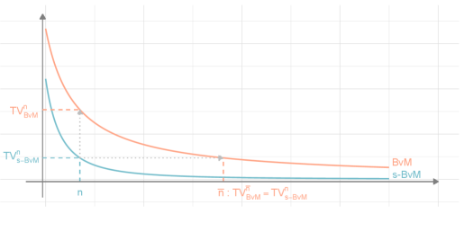
Under the above assumptions, Theorem 2.1 below provides theoretical support to the proposed sks approximation by stating a novel skewed Bernstein–von Mises type result. More specifically, this result establishes that in general contexts, covering also misspecified models and non–i.i.d. settings, it is possible to derive a sks approximation, with density as in (1), whose tv distance from the target posterior has a rate which improves by at least one order of magnitude the one achieved by the classical Gaussian counterpart from the Bernstein–von Mises theorem. By approaching the target posterior at a provably–faster rate, the proposed solution is therefore expected to provide, in practice, a more accurate alternative to Gaussian approximations of the target posterior, while inheriting the corresponding limiting frequentist properties. To this end, Theorem 2.1 shall not be interpreted as a theoretical result aimed at providing novel or alternative frequentist support to Bayesian inference. Rather, it represents an important refinement of the classical Bernstein–von Mises theorem which guides and supports the derivation of improved deterministic approximations to be used in practice as tractable, yet accurate, alternatives to the intractable posterior of direct interest. Figure 1 provides a graphical intuition for such an argument. The practical impact of these results is illustrated in the empirical studies within Sections 3 and 5. Such studies clarify that the theoretical improvements encoded in the rates we derive directly translate into the remarkable accuracy gains of the proposed class of sks approximations observed in finite–sample studies.

Theorem 2.1.

Let $h=\delta_{n}^{-1}(\theta-\theta_{*}),$ and define $M_{n}=\sqrt{c_{0}\log\delta_{n}^{-1}}$ , with $c_{0}>0$ . Then, under Assumptions 1–4, if $\theta_{*}$ is an inner point of $\Theta$ , it holds

\displaystyle\|\Pi_{n}(\cdot)-P_{\textsc{sks}}^{n}(\cdot)\|_{\textsc{tv}}=O_{P_{0}^{n}}(M_{n}^{c_{3}}\delta_{n}^{2}),

(8)

where $c_{3}>0$ , and $P_{\textsc{sks}}^{n}(\cdot)$ is the cdf of the sks density $p_{\textsc{sks}}^{n}(h)$ in (1) with parameters

\displaystyle\begin{split}&\xi=\Delta_{\theta_{*}}^{n}+\delta_{n}(V^{n}_{\theta_{*}})^{-1}\log\pi^{(1)},\qquad\Omega^{-1}=[v_{st}^{n}-\delta_{n}\smash{a^{(3),n}_{\theta_{*},stl}}\xi_{l}],\\ &\alpha_{\eta}(h-\xi)=(\delta_{n}/12\eta)\smash{a^{(3),n}_{\theta_{*},stl}}\{(h-\xi)_{s}(h-\xi)_{t}(h-\xi)_{l}+3(h-\xi)_{s}\xi_{t}\xi_{l}\}.\end{split}

The function $F(\cdot)$ entering the definition of $p_{\textsc{sks}}^{n}(h)$ in (1) is any univariate cdf which satisfies $F(-x)=1-F(x)$ and $F(x)=1/2+\eta x+O(x^{2})$ , for some $\eta\in\mathbb{R}$ , when $x\to 0$ .

Remark 2.2.

Under related conditions and a simpler proof, it is possible to show that the order of convergence for the Bernstein–von Mises theorem based on limiting Gaussians is $O_{P_{0}^{n}}(M_{n}^{c_{4}}\delta_{n})$ , for some $c_{4}>0$ . Thus, Theorem 2.1 guarantees that by relying on suitably–derived sks approximations with density as in (1), it is possible to improve the rates of the classical Bernstein–von Mises result by a multiplicative factor of $\delta_{n}$ . This follows directly from the fact that the sks approximation is able to include terms of order $\delta_{n}$ that are present in the Taylor expansion of the log–posterior but are neglected in the Gaussian limit. This allows an improved redistribution of the mass in the high posterior probability region, thereby yielding increased accuracy in characterizing the shape of the target posterior. As illustrated in Sections 3 and 5, this correction yields remarkable accuracy improvements in practice.

Remark 2.3.

Theorem 2.1 holds for a broad class of sks approximating distributions as long as the univariate cdf $F(\cdot)$ which enters the skewing factor in (1) satisfies $F(-x)=1-F(x)$ and $F(x)=1/2+\eta x+O(x^{2})$ for some $\eta\in\mathbb{R}$ when $x\to 0$ . These conditions are mild and add flexibility in the selection of $F(\cdot)$ . Relevant and practical examples of possibile choices for $F(\cdot)$ are the cdf of the standard Gaussian distribution, $\Phi(\cdot)$ , and the inverse logit function, $g(\cdot)=\exp(\cdot)/\{1+\exp(\cdot)\}$ . Both satisfy $F(-x)=1-F(x)$ , and the associated Taylor expansions are $\Phi(x)=1/2+x/\sqrt{2\pi}+O(x^{3})$ and $g(x)=1/2+x/4+O(x^{3})$ , respectively, for $x\to 0$ . Interestingly, when $F(\cdot)=\Phi(\cdot)$ , the resulting skew–symmetric approximation belongs to the well–studied sub–class of generalized skew–normal (gsn) distributions (Ma and Genton, 2004), which provide the most natural extension of multivariate skew–normals (Azzalini and Capitanio, 2003) to more flexible skew–symmetric representations. Due to this, Sections 3 and 5 focus on assessing the empirical performance of such a noticeable example.

Before entering the details of the proof of Theorem 2.1, let us highlight an interesting aspect regarding the interplay between skew–symmetric and Gaussian approximations that can be deduced from our theoretical studies. In particular, notice that Theorem 2.1 states results in terms of approximation of the whole posterior distribution under the tv distance. This implies, as a direct consequence of the definition of such a distance, that the same rates hold also for the absolute error in approximating the posterior expectation of any bounded function. As shown later in Corollary 2.5, such an improvement can also be proved, under mild additional conditions, for the approximation of the posterior expectation of any function bounded by a polynomial (e.g., posterior moments). According to Remark 2.2 these rates cannot be achieved in general under a Gaussian approximation. Nonetheless, as stated in Lemma 2.4, for some specific functionals the classical Gaussian approximation can actually attain the same rates of its skewed version. This result follows from the skew–symmetric distributional invariance with respect to even functions (Wang, Boyer and Genton, 2004). Such a property implies that the sks approximation $2\phi_{d}\left(h;\xi,\Omega\right)F(\alpha_{\eta}(h-\xi))$ and its Gaussian component $\phi_{d}\left(h;\xi,\Omega\right)$ yield the same level of accuracy in estimating the posterior expected value of functions that are symmetric with respect to the location parameter $\xi$ . Thus, our results provide also a novel explanation of the phenomenon observed in Spokoiny and Panov (2021) and Spokoiny (2023), where the quality of the Gaussian approximation, within high–dimensional models, increases by an order of magnitude when evaluated on Borel sets which are centrally symmetric with respect to the location $\xi$ (e.g., Spokoiny, 2023, Theorem 3.4). Nonetheless, as clarified in Theorem 2.1 and Remark 2.2, Gaussian approximations remain still unable to attain the same rates of the sks counterparts in the estimation of generic functionals. Relevant examples are highest posterior density intervals which are often studied in practice and will be non–symmetric by definition whenever the posterior is skewed.

Lemma 2.4.

Let $2\phi_{d}(h;\xi,\Omega)F(\alpha_{\eta}(h-\xi))$ with $\xi\in\mathbb{R}^{d}$ and $\Omega\in\mathbb{R}^{d}\times\mathbb{R}^{d}$ , be a skew-symmetric approximation of $\pi_{n}(h)$ and let $G\,:\,\mathbb{R}^{d}\to\mathbb{R}$ be an even function. If both $\int G(h-\xi)\pi_{n}(h)dh$ and $\int G(h-\xi)2\phi_{d}(h;\xi,\Omega)F(\alpha_{\eta}(h-\xi))dh$ are finite, it holds

\displaystyle{\int}G(h-\xi)\{\pi_{n}(h)-2\phi_{d}(h;\xi,\Omega)F(\alpha_{\eta}(h-\xi))\}dh\ {=}{\int}G(h-\xi)\{\pi_{n}(h)-\phi_{d}(h;\xi,\Omega)\}dh.

As clarified in the Supplementary Materials, Lemma 2.4 follows as a direct consequence of Proposition 6 in Wang, Boyer and Genton (2004).

The proof of Theorem 2.1 is reported below and extends to sks approximating distributions the reasoning behind the derivation of general Bernstein–von Mises type results (Kleijn and van der Vaart, 2012). Nonetheless, as mentioned before, the need to derive sharper rates which establish a higher approximation accuracy, relative to Gaussian limiting distributions, requires a number of additional technical lemmas and refined arguments ensuring a tighter control of the error terms in the expansions behind Theorem 2.1. Note also that, in addressing these aspects, it is not sufficient to rely on standard theory for higher–order approximations. In fact, unlike for current results, Theorem 2.1 establishes improved rates for a valid class of approximating densities. This means that, beside replacing the second–order expansion of the log–posterior with a third–order one, it is also necessary to carefully control the difference between such an expansion and the class of sks distributions.

Proof.

Let $p_{\textsc{sks}}^{n}(h)$ denote the sks density in (1) with parameters derived in Lemma B.1 under Assumptions 2 and 3 (see the Supplementary Materials). In addition, let $\pi_{n}^{K_{n}}(h)$ and $p_{\textsc{sks}}^{n,K_{n}}(h)$ be the constrained versions of $\pi_{n}(h)$ and $p_{\textsc{sks}}^{n}(h)$ to the set $K_{n}=\{h{:}\ ||h||<~{}M_{n}\}$ , i.e, $\smash{\pi_{n}^{K_{n}}(h)}=\pi_{n}(h)\mathbbm{1}_{h\in K_{n}}/\Pi_{n}(K_{n})$ and $p_{\textsc{sks}}^{n,K_{n}}(h)=p_{\textsc{sks}}^{n}(h)\mathbbm{1}_{h\in K_{n}}/P_{\textsc{sks}}^{n}(K_{n})$ . Using triangle inequality

\displaystyle\begin{aligned} \quad&\|\Pi_{n}(\cdot)-P_{\textsc{sks}}^{n}(\cdot)\|_{\textsc{tv}}=\frac{1}{2}\int|\pi_{n}(h)-p_{\textsc{sks}}^{n}(h)|dh\leq\\ &\quad\ \ {\int}|\pi_{n}(h)-\pi_{n}^{K_{n}}(h)|dh\ {+}{\int}|\pi_{n}^{K_{n}}(h)-p_{\textsc{sks}}^{n,K_{n}}(h)|dh\ {+}{\int}|p_{\textsc{sks}}^{n}(h)-p_{\textsc{sks}}^{n,K_{n}}(h)|dh,\end{aligned}

(9)

the proof of Theorem 2.1 reduces to study the behavior of the three above summands.

As for the first term, Assumption 4 and a standard inequality of the tv norm yield

\displaystyle\int|\pi_{n}(h)-\pi_{n}^{K_{n}}(h)|dh\leq 2\int_{h\,:\,\|h\|>M_{n}}\pi_{n}(h)dh=O_{P_{0}^{n}}(\delta_{n}^{2}).

(10)

Let us now deal with the third term via a similar reasoning. More specifically, leveraging the same tv inequality as above and the fact that $F(\alpha_{\eta}(h-\xi))$ within the expression for $p_{\textsc{sks}}^{n}(h)$ in (1) is a univariate cdf meeting the condition $|F(\alpha_{\eta}(h-\xi))|\leq 1$ , we have

\displaystyle{\int}|p_{\textsc{sks}}^{n}(h)-p_{\textsc{sks}}^{n,K_{n}}(h)|dh\leq 4\int_{h\,:\,\|h\|>M_{n}}\phi_{d}(h;\xi,\Omega)dh.

Define $P_{\xi,\Omega}(\|h\|>M_{n}):=$ $\smash{\int_{h\in K_{n}^{c}}\phi_{d}(h;\xi,\Omega)dh}$ and let $A_{n,1}=\{\lambda_{\textsc{min}}(\Omega)>\eta_{1}\}\cap\{\lambda_{\textsc{max}}(\Omega)$ $<\eta_{2}\}\cap\{\|\xi\|<\tilde{M}_{n}\}$ for some sequence $\tilde{M}_{n}=o(M_{n})$ going to infinity arbitrary slowly and some $\eta_{1},\eta_{2}>0$ . Moreover, notice that $V_{\theta_{*}}^{n}-\Omega^{-1}$ has entries of order $O_{P_{0}^{n}}(\delta_{n})$ . As a consequence, in view of Assumptions 2–3 and Lemma B.2 in the Supplementary Materials, it follows that $P_{0}^{n}A_{n,1}=1-o(1)$ . Conditioned on $A_{n,1}$ , the eigenvalues of $\Omega$ lay on a positive bounded range. This, together with $\tilde{M}_{n}/M_{n}\to 0$ , imply

\displaystyle\begin{aligned} \quad P_{0}^{n}(P_{\xi,\Omega}(\|h\|>M_{n})/\delta_{n}^{2}>\epsilon)\,=&\,P_{0}^{n}(\{P_{\xi,\Omega}(\|h\|>M_{n})/\delta_{n}^{2}>\epsilon\}\cap A_{n,1})+o(1)\\ &\leq P_{0}^{n}(e^{-\tilde{c}_{1}M_{n}^{2}}/\delta_{n}^{2}>\epsilon\mid A_{n,1})+o(1)=o(1),\end{aligned}

(11)

for every $\epsilon>0$ , where $\tilde{c}_{1}$ is a sufficiently small positive constant and the last inequality follows from the tail behavior of the multivariate Gaussian for a sufficiently large choice of $c_{0}$ in $M_{n}=\sqrt{c_{0}\log\delta_{n}^{-1}}$ . This gives

\displaystyle{\int}|p_{\textsc{sks}}^{n}(h)-p_{\textsc{sks}}^{n,K_{n}}(h)|dh\leq 4\int_{h\,:\,\|h\|>M_{n}}\phi_{d}(h;\xi,\Omega)dh=o_{P_{0}^{n}}(\delta_{n}^{2}).

(12)

We are left to study the last summand ${\int}|\pi_{n}^{K_{n}}(h)-p_{\textsc{sks}}^{n,K_{n}}(h)|dh$ . To this end, let us consider the event $A_{n,2}=A_{n,1}\cap\{\Pi_{n}(K_{h})>0\}\cap\{P_{\textsc{sks}}^{n}(K_{n})>0\}.$ Notice that

P_{0}^{n}(\Pi_{n}(K_{h})>0)=1-o(1)

by Assumption 4. Moreover, in view of (11), it follows that $P_{0}^{n}(P_{\textsc{sks}}^{n}(K_{n})>0)=P_{0}^{n}(1-P_{\textsc{sks}}^{n}(K^{c}_{n})>0)\geq P_{0}^{n}(1-2P_{\xi,\Omega}(\|h\|>M_{n})>0)=1-o(1),$ implying, in turn, $P_{0}^{n}A_{n,2}=1-o(1)$ . As a consequence, we can restrict our attention to

\displaystyle\begin{aligned} \qquad&\int|\pi_{n}^{K_{n}}(h)-p_{\textsc{sks}}^{n,K_{n}}(h)|dh\mathbbm{1}_{A_{n,2}}\\ &=\int\Big{|}1-\int_{K_{n}}\frac{p_{\textsc{sks}}^{n,K_{n}}(h)}{p_{\textsc{sks}}^{n,K_{n}}(h^{\prime})}\frac{p_{\theta_{*}+\delta_{n}h^{\prime}}(X^{n})\pi(\theta_{*}+\delta_{n}h^{\prime})}{p_{\theta_{*}+\delta_{n}h}(X^{n})\pi(\theta_{*}+\delta_{n}h)}p_{\textsc{sks}}^{n,K_{n}}(h^{\prime})dh^{\prime}\Big{|}\pi_{n}^{K_{n}}(h)dh\mathbbm{1}_{A_{n,2}}.\end{aligned}

(13)

Now, note that, by the definition of $p_{\textsc{sks}}^{n,K_{n}}(h)$ , we have $p_{\textsc{sks}}^{n,K_{n}}(h)/p_{\textsc{sks}}^{n,K_{n}}(h^{\prime})=p_{\textsc{sks}}^{n}(h)/p_{\textsc{sks}}^{n}(h^{\prime})$ . This fact, together with an application of Jensen’s inequality, implies that the quantity on the right hand side of Equation (13) can be upper bounded by

\displaystyle\begin{aligned} &\int_{K_{n}\times K_{n}}\Big{|}1-\frac{p_{\textsc{sks}}^{n}(h)}{p_{\textsc{sks}}^{n}(h^{\prime})}\frac{p_{\theta_{*}+\delta_{n}h^{\prime}}(X^{n})\pi(\theta_{*}+\delta_{n}h^{\prime})}{p_{\theta_{*}+\delta_{n}h}(X^{n})\pi(\theta_{*}+\delta_{n}h)}\Big{|}\pi_{n}^{K_{n}}(h)p_{\textsc{sks}}^{n,K_{n}}(h^{\prime})dhdh^{\prime}\mathbbm{1}_{A_{n,2}}.\\ \end{aligned}

At this point, it is sufficient to recall Lemma B.1 within the Supplementary Materials and the fact that $e^{x}=1+x+e^{\beta x}x^{2}/2$ , for some $\beta\in(0,1)$ , to obtain

	$\displaystyle{\int}\|\pi_{n}^{K_{n}}(h)-p_{\textsc{sks}}^{n,K_{n}}(h)\|dh\mathbbm{1}_{A_{n,2}}$	$\displaystyle\leq$	$\displaystyle{\int_{K_{n}\times K_{n}}}\|1-e^{r_{n,4}(h^{\prime})-r_{n,4}(h)}\|\pi_{n}^{K_{n}}(h)p_{\textsc{sks}}^{n,K_{n}}(h^{\prime})dhdh^{\prime}\mathbbm{1}_{A_{n,2}}$		(14)
		$\displaystyle\leq$	$\displaystyle 2\|r_{n,4}\|+2\exp(2\beta\|r_{n,4}\|)r_{n,4}^{2}=O_{P_{0}^{n}}(\delta_{n}^{2}M_{n}^{c_{3}}),$		(14)

where $r_{n,4}=\sup_{h\in K_{n}}r_{n,4}(h)$ , and $c_{3}$ is some constant defined in Lemma B.1. We conclude the proof by noticing that the combination of (9), (10), (12) and (14), yields Equation (8) in Theorem 2.1. ∎

2.3 Skew–symmetric approximations in regular parametric models

Theorem 2.1 states a general result under broad assumptions. In this section, we strengthen the methodological and practical impact of such a result by specializing the analysis to the context of, possibly misspecified and non–i.i.d., regular parametric models with $d$ fixed and $\delta_{n}=n^{-1/2}$ . The focus on this practically–relevant setting crucially clarifies that Assumptions 1–4 can be readily verified under standard explicit conditions on the log–likelihood and log–prior derivatives, which in turn enter the definition of the sks parameters $\xi$ , $\Omega$ and $\alpha_{\eta}(h-\xi)$ . This allows direct and closed–form derivation of $p_{\textsc{sks}}^{n}(h)$ in routine implementations of deterministic approximations for intractable posteriors induced by broad classes of parametric models. As stated in Corollary 2.5, in this setting the resulting sks approximating density achieves a remarkable improvement in the rates by a $\sqrt{n}$ factor, up to a poly–log term, relative to the classical Gaussian approximation. This accuracy gain can be proved both for the tv distance from the target posterior and also for the absolute error in the approximation for the posterior expectation of general polynomially bounded functions, with finite prior expectation.

Prior to stating Corollary 2.5, let us introduce a number of explicit assumptions which allow to specialize the general theory in Section 2.2 to the setting with $d$ fixed and $\delta_{n}=n^{-1/2}$ . As discussed in the following, Assumptions 5–6 provide natural and verifiable conditions which ensure that the general Assumptions 2–4 are met, thereby allowing Theorem 2.1 to be applied, and specialized, to the regular parametric models setting.

Assumption 5.

Define $\ell^{(4)}_{\theta_{*},stlk}(h):=\ell_{stlk}^{(4)}(\theta_{*}+h/\sqrt{n})$ . Then, the log–likelihood of the, possibly misspecified, model is four times differentiable at $\theta_{*}$ with

\displaystyle\ell^{(1)}_{\theta_{*},s}=O_{P_{0}^{n}}(n^{1/2}),\quad\ell^{(2)}_{\theta_{*},st}=O_{P_{0}^{n}}(n),\quad\ell^{(3)}_{\theta_{*},stl}=O_{P_{0}^{n}}(n),\quad\mbox{for }\ s,t,l=1,\ldots,d,

and $\sup_{h\in K_{n}}|\ell^{(4)}_{\theta_{*},stlk}(h)|=O_{P_{0}^{n}}(n)$ , for $s,t,l,k=1,\ldots,d$ .

Assumption 6.

The entries of the expected Fisher information matrix satisfy $i_{st}=~{}O(n)$ while $j_{st}/n-i_{st}/n=\smash{O_{P_{0}^{n}}(n^{-1/2})}$ , for $s,t=1,\dots,d.$ Moreover, there exist two positive constants $\eta_{1}$ and $\eta_{2}$ such that $\lambda_{\textsc{min}}(I_{\theta_{*}}/n)>\eta_{1}$ and $\lambda_{\textsc{max}}(I_{\theta_{*}}/n)<\eta_{2}$ .

Assumption 7.

The log–prior density $\log\pi(\theta)$ is two times continuously differentiable in a neighborhood of $\theta_{*}$ , and $0<\pi(\theta_{*})<\infty$ .

Assumption 8.

For every sequence $M_{n}\to\infty$ there exists a constant $c_{5}>0$ such that $\lim_{n\to\infty}P_{0}^{n}\{\sup_{\|\theta-\theta_{*}\|>M_{n}/\sqrt{n}}\{(\ell(\theta)-\ell(\theta_{*}))/n\}<-c_{5}M_{n}^{2}/n\}=1.$

Assumptions 5–6 are mild and considered standard in classical frequentist theory (see e.g., Pace and Salvan, 1997, p. 347). In Lemma 2.8 we show that these conditions allow to control with precision the error in the Taylor approximation of the log–likelihood. Assumption 7 is also mild and is satisfied by several priors that are commonly used in practice. Such a condition allows to consider a first order Taylor expansion for the log–prior of the form

\displaystyle\log\pi(\theta)=\log\pi(\theta_{*})+\log\pi^{(1)}_{\theta_{*},s}h_{s}/\sqrt{n}+r_{n,2}(h),

(15)

with $r_{n,2}:=\sup_{h\in K_{n}}r_{n,2}(h)=O(M_{n}^{2}/n)$ . Finally, Assumption 8 is required to control the the rate of contraction of the, possibly misspecified, posterior distribution into $K_{n}$ . In other modern versions of Berstein–Von Mises type results, such an assumption is usually replaced by conditions on the existence of a suitable sequence of tests. Sufficient conditions for the correctly–specified case can be found, for example, in Van der Vaart (2000). In the misspecified setting, assumptions ensuring the existence of these tests have been derived by Kleijn and van der Vaart (2012). Another possible option is to assume, for every $\delta>0$ , the presence of a positive constant $c_{\delta}$ such that

\displaystyle\lim_{n\to\infty}P_{0}^{n}\{{\textstyle\sup_{\|\theta-\theta_{*}\|>\delta}}\{(\ell(\theta)-\ell(\theta_{*}))/n\}<-c_{\delta}\}=1.

(16)

In the misspecified setting, condition (16) is considered by, e.g., Koers, Szabo and van der Vaart (2023). Assumption 8 is a slightly more restrictive version of (16). In fact, Lemma 2.10 below shows that it is implied by mild and readily–verifiable sufficient conditions.

Under Assumption 1 and 5–8, Corollary 2.5 below clarifies that Theorem 2.1 holds for a general class of sks distributions yielding tv rates in approximating the exact posterior of order $O_{P_{0}^{n}}(M_{n}^{c_{6}}/n)$ , with $c_{6}>0$ and $M_{n}=\sqrt{c_{0}\log n}$ . Furthermore, the sks parameters are defined as explicit functions of the log–prior and log–likelihood derivatives. As stated in Equation (18) of Corollary 2.5, the same rates can be derived also for the absolute error in approximating the posterior expectation of general polynomially bounded functions.

Corollary 2.5.

Let $h=\sqrt{n}(\theta-\theta_{*}),$ and define $M_{n}=\sqrt{c_{0}\log n}$ , with $c_{0}>0$ . Then, under Assumptions 1 and 5–8 it holds

\displaystyle\|\Pi_{n}(\cdot)-P_{\textsc{sks}}^{n}(\cdot)\|_{\textsc{tv}}=O_{P_{0}^{n}}(M_{n}^{c_{6}}/n).

(17)

where $c_{6}>0$ , and $P_{\textsc{sks}}^{n}(\cdot)$ is the cdf of the sks density $p_{\textsc{sks}}^{n}(h)$ in (1) with parameters

\displaystyle\begin{split}&\xi=\smash{[n(J^{-1}_{\theta_{*}})_{st}u_{t}]},\qquad\Omega^{-1}=[j_{st}/n-(\xi_{l}\ell^{(3)}_{\theta_{*},stl}/n)/\sqrt{n}],\\ &\alpha_{\eta}(h-\xi)={\{}1/(12\eta\sqrt{n})\}(\ell^{(3)}_{\theta_{*},stl}/n)\{(h-\xi)_{s}(h-\xi)_{t}(h-\xi)_{l}+3(h-\xi)_{s}\xi_{t}\xi_{l}\}.\end{split}

where $\smash{u_{t}=(\ell^{(1)}_{\theta_{*}}+\log\pi^{(1)}_{\theta_{*}})_{t}/\sqrt{n}}$ for $t=1,\ldots,d$ . The function $F(\cdot)$ entering the definition of $p_{\textsc{sks}}^{n}(h)$ in (1) denotes any univariate cdf which satisfies $F(-x)=1-F(x)$ and $F(x)=1/2+\eta x+O(x^{2})$ , for some $\eta\in\mathbb{R}$ , when $x\to 0$ . In addition, let $G\,:\,\mathbbm{R}^{d}\to R$ be a function satisfying $|G|\lesssim\|h\|^{r}$ . If the prior is such that $\int\|h\|^{r}\pi(\theta+h/\sqrt{n})dh<\infty$ then

\displaystyle\int G(h)|\pi_{n}(h)-p_{\textsc{sks}}^{n}(h)|dh=O_{P_{0}^{n}}(M_{n}^{c_{6}+r}/n).

(18)

with $p_{\textsc{sks}}^{n}(h)$ denoting the skew–symmetric approximating density defined above.

Remark 2.6.

As for Theorem 2.1, under conditions similar to those required by Corollary 2.5, it is possible to show that the tv distance between the posterior and the Gaussian approximation dictated by the classical Bernstein–von Mises theorem is $O_{P_{0}^{n}}(M_{n}^{c_{7}}/\sqrt{n})$ for some fixed $c_{7}>0$ . Therefore, the improvement in rates achieved by the proposed sks approximation is by a remarkable $\sqrt{n}$ factor, up to a poly–log term. As illustrated in Figure 1, this implies that the sks solution is expected to substantially improve, in practice, the accuracy of the classical Gaussian in approximating the target posterior, while inheriting its limiting frequentist properties. Intuitively, the rates we derive suggest that the proposed sks approximation can possibly attain with a $n\approx\sqrt{\bar{n}}$ sample size the same accuracy obtained by its Gaussian counterpart with a sample size of $\bar{n}$ . The empirical studies in Sections 3 and 5 confirm this intuition, which is further strengthened in Section 4 through the derivation of non–asymptotic upper bounds for the practical skew–modal approximation, along with novel lower bounds for the classical Gaussian from the Laplace method.

Remark 2.7.

Equation (18) confirms that the improved rates hold also when the focus is on the error in approximating the posterior expectation of generic polynomially bounded functions. More specifically, notice that, by direct application of standard properties of integrals, the proof of Equation (18) in the Supplementary Materials, implies

\displaystyle\textstyle\big{|}\int G(h)\pi_{n}(h)dh-\int G(h)p_{\textsc{sks}}^{n}(h)dh|=O_{P_{0}^{n}}(M_{n}^{c_{6}+r}/n).

(19)

This clarifies that the skewed Bernstein–von Mises type result in (17) has important methodological and practical consequences that point toward remarkable improvements in the approximation of posterior functionals of direct interest for inference (e.g., moments).

Refer to caption — Figure 1: Illustrative graphical comparison among the tv–rates achieved by the proposed skew–symmetric approximation (s–BvM) and those derived under the classical Bernstein–von Mises theorem based on Gaussians (BvM). For a given $n$ , we show the tv distances $\textsc{tv}_{\textsc{s--BvM}}^{n}$ and $\textsc{tv}_{\textsc{BvM}}^{n}$ expected under the s–BvM and BvM rates, respectively. We further highlight the expected sample size $\bar{n}\gg n$ required by BvM to attain the same tv distance as the one achieved by s–BvM with the original $n$ , under the derived rates. The empirical studies in Sections 3 and 5 support this graphical intuition.

The proof of Equation (18) can be found in the Supplementary Materials. As for the main result in Equation (17), it is sufficient to apply Theorem 2.1, after ensuring that its Assumptions 1–4 are implied by 1 and 5–8. Section 2.3.1 presents two key results (see Lemma 2.8 and Lemma 2.9) which address this point. Section 2.3.2 introduces instead simple and verifiable conditions which ensure the validity of Assumption 8.

2.3.1 Log–posterior asymptotics and posterior contraction

In order to move from the general theory within Theorem 2.1 to the specialized setting considered in Corollary 2.5, two key points are the rate at which the target posterior concentrates in $K_{n}=\{h\,:\,\|h\|<M_{n}\}$ and the behavior of the Taylor expansion of the log–likelihood within $K_{n}$ . Here we show that Assumptions 1 and 5–8 are indeed sufficient to obtain the required guarantees. Lemma 2.8 below establishes that, under Assumptions 5–6, the error introduced by replacing the log–likelihood with its third–order Taylor approximation is uniformly of order $M_{n}^{4}/n$ on $K_{n}$ .

Lemma 2.8.

Under Assumptions 5–6, it holds in $K_{n}=\{h\,:\,\|h\|\leq M_{n}\}$ that

\displaystyle\log\frac{p_{\theta_{*}+h/\sqrt{n}}^{n}}{p_{\theta_{*}}^{n}}(X^{n})-h_{s}v_{st}^{n}\Delta_{\theta_{*},t}^{n}+\frac{1}{2}v_{st}^{n}h_{s}h_{t}-\frac{1}{6\sqrt{n}}a^{(3),n}_{\theta_{*},stl}h_{s}h_{t}h_{l}=r_{n,1}(h),

(20)

with $\Delta_{\theta_{*},t}^{n}=j^{-1}_{st}\sqrt{n}\ell^{(1)}_{\theta_{*},s}=O_{P_{0}^{n}}(1),$ $v_{st}^{n}=j_{st}/n=O_{P_{0}^{n}}(1)$ and $a^{(3),n}_{\theta_{*},stl}=\ell^{(3)}_{\theta_{*},stl}/n=O_{P_{0}^{n}}(1)$ . Moreover, $r_{n,1}:=\sup_{h\in K_{n}}\left|r_{n,1}(h)\right|=O_{P_{0}^{n}}(M_{n}^{4}/n)$ .

Lemma 2.9 shows that under the above conditions it is then possible to select $c_{0}$ in $M_{n}=\sqrt{c_{0}\log n}$ , and hence $K_{n}$ , such that the posterior distribution concentrates its mass in $K_{n}$ , at any polynomial rate, with $P_{0}^{n}$ probability tending to 1 as $n\to\infty$ . This in turn implies that Assumption 4 in Section 2.2 is satisfied.

Lemma 2.9 (Posterior contraction).

Under Assumptions 5–8, there exists a sufficiently–large $c_{0}>0$ in $M_{n}=\sqrt{c_{0}\log n}$ , such that for every $D>0$ it holds

\displaystyle\lim_{n\to\infty}P_{0}^{n}\{\Pi_{n}(K_{n}^{c})<n^{-D}\}=1,

where $K_{n}^{c}$ is the complement of $K_{n}$ .

To complete the connection between Theorem 2.1 and Corollary 2.5, note that Assumption 7 implies that Assumption 3 in Section 2.2 is verified with $\log\pi^{(1)}=(\partial/\partial\theta)\log\pi(\theta)_{|\theta=\theta_{*}}$ . Refer to the Supplementary Materials for the proofs of Lemma 2.8 and Lemma 2.9.

2.3.2 Sufficient conditions for Assumption 8

Lemma 2.9 requires the fulfillment of Assumption 8 which allows precise control on the behavior of the log–likelihood ratio outside the set $K_{n}$ . In addition, Assumption 8 further plays a crucial role in the development of the practical skew–modal approximation presented in Section 4. Given the relevance of such an assumption, Lemma 2.10 provides a set of natural and verifiable sufficient conditions that guarantee its validity; see the Supplementary Materials for the proof of Lemma 2.10.

Lemma 2.10.

Suppose that Assumptions 1 and 6 hold, and that for every $\delta>0$ there exists a positive constant $c_{\delta}$ such that

\displaystyle\textstyle\lim_{n\to\infty}P_{0}^{n}\{\sup_{\|\theta-\theta_{*}\|>\delta}\{(\ell(\theta)-\ell(\theta_{*}))/n\}<-c_{\delta}\}=1.

(21)

If there exist $\bar{n}\in\mathbbm{N}$ and $\delta_{1}>0$ such that, for all $n>\bar{n}$ , it holds

•

R1) $\mathbb{E}_{0}^{n}\{\ell(\theta)-\ell(\theta_{*})\}/n$ is concave in $\{\theta\,:\,\|\theta-\theta_{*}\|<\delta_{1}\}$ , two times differentiable at $\theta_{*}$ with negative Hessian equal to the expected Fisher information matrix $I_{\theta_{*}}/n,$
•

R2) and $\sup_{0<\|\theta-\theta_{*}\|<\delta_{1}}[\{\ell(\theta)-\ell(\theta_{*})\}-\mathbb{E}_{0}^{n}\{\ell(\theta)-\ell(\theta_{*})\}]/(n\|\theta-\theta_{*}\|)=O_{P_{0}^{n}}(n^{-1/2}),$

then there is a constant $c_{5}>0$ such that $\lim_{n\to\infty}P_{0}^{n}\{\sup_{\|\theta-\theta_{*}\|>M_{n}/\sqrt{n}}\{(\ell(\theta)-\ell(\theta_{*}))/n\}<-c_{5}M_{n}^{2}/n\}=1$ , for any $M_{n}\to\infty$ .

As highlighted at the beginning of Section 2.3, condition (21) is mild and can be found both in classical (e.g., Lehmann and Casella, 2006) and modern (Koers, Szabo and van der Vaart, 2023) Bernstein–von Mises type results. Condition R1 requires the expected log–likelihood to be sufficiently regular within a neighborhood of $\theta_{*}$ and is closely related to standard assumptions on M–estimators (e.g., Van der Vaart, 2000, Ch. 5). Finally, among the assumptions of Lemma 2.10, R2 is arguably the most specific. It requires that, for all $\theta$ such that $0<\|\theta-\theta_{*}\|<\delta_{1}$ , the quantity $[\{\ell(\theta)-\ell(\theta_{*})\}-\mathbb{E}_{0}^{n}\{\ell(\theta)-\ell(\theta_{*})\}]/(n\|\theta-\theta_{*}\|)$ converges uniformly to zero in probability with rate $n^{-1/2}$ . This type of behavior is common in several routinely–implemented statistical models, such as generalized linear models.

3 Empirical results

Sections 3.1–3.2 provide empirical evidence of the improved accuracy achieved by the sks approximation in Corollary 2.5 (s–BvM), relative to its Gaussian counterpart (BvM) arising from the classical Bernstein–von Mises theorem in regular parametric models. We study both correctly–specified and misspecified settings, and focus not only on assessing the superior performance of the sks approximation, with $F(\cdot)=\Phi(\cdot)$ , but also on quantifying whether the remarkable improvements encoded in the rates we derived under asymptotic arguments find empirical evidence also in finite–sample studies. To this end, s–BvM and BvM are compared both in terms of tv distance from the target posterior and also with respect to the absolute error in approximating the posterior mean. These two measures illustrate the practical implications of the rates derived in Equation (17) and (18), respectively. Since for the illustrative studies in Sections 3.1 and 3.2 the target posterior can be derived in closed form, the tv distances $\textsc{tv}^{n}_{\textsc{BvM}}=(1/2)\int_{\mathbbm{R}}|\pi_{n}(h)-p^{n}_{\textsc{gauss}}(h)|dh$ and $\textsc{tv}^{n}_{\textsc{s--BvM}}=(1/2)\int_{\mathbbm{R}}|\pi_{n}(h)-p^{n}_{\textsc{sks}}(h)|dh$ can be evaluated numerically, for every $n$ , via standard routines in R. The same holds for the errors in posterior mean approximation $\textsc{fmae}^{n}_{\textsc{BvM}}=|\int_{\mathbbm{R}}h\{\pi_{n}(h)-p^{n}_{\textsc{gauss}}(h)\}dh|$ and $\textsc{fmae}^{n}_{\textsc{s--BvM}}=|\int_{\mathbbm{R}}h\{\pi_{n}(h)-p^{n}_{\textsc{sks}}(h)\}dh|$ .

Note that, as for other versions of the classical Bernstein–von Mises theorem, also our theoretical results in Sections 2.2 and 2.3 require knowledge of the Kullback–Leibler minimizer between the true data–generating process and the parametric family $\mathcal{P}_{\Theta}$ . Since $\theta_{*}$ is clearly unknown in practice, in Section 4 we address this aspect via a practical plug–in version of the sks approximation in Corollary 2.5, which replaces $\theta_{*}$ with its maximum a posteriori estimate. This yields a readily–applicable skew–modal approximation with similar theoretical and empirical support; see the additional simulations and real–data applications in Section 5.

3.1 Exponential model

Let $X_{i}\stackrel{{\scriptstyle iid}}{{\sim}}\textsc{exp}(\theta_{0})$ , for $i=1,\ldots,n$ , where $\textsc{exp}(\theta_{0})$ denotes the exponential distribution with rate parameter $\theta_{0}=2.$ In the following, we consider a correctly specified model having exponential likelihood and a $\textsc{exp}(1)$ prior for $\theta$ . To obtain the skew–symmetric approximation for the posterior distribution induced by such a Bayesian model, let us first verify that all conditions of Corollary 2.5 hold.

To address this goal first note that, as the model is correctly specified, Assumption 1 holds with $\theta_{*}=\theta_{0}$ . The first four derivates of the log–likelihood at $\theta$ are $n/\theta-\sum_{i=1}^{n}x_{i},$ $-n/\theta^{2}$ , $2n/\theta^{3}$ and $-6n/\theta^{4}$ , respectively. Hence, Assumptions 5–6 are both satisfied, even around a small neighborhood of $\theta_{0}$ . Assumption 7 is met by a broad class of routinely–implemented priors. For example, $\textsc{exp}(1)$ can be considered in such a case. Finally, we need to check Assumption 8. To this end, note that $\{\ell(\theta)-\ell(\theta_{0})\}/n=\log\theta/\theta_{0}+(\theta_{0}-\theta)\sum_{i=1}^{n}x_{i}/n$ which, by the law of large number, converges in probability to a negative constant for every fixed $\theta$ implying (21). Additionally, $\mathbb{E}_{0}^{n}\{\ell(\theta)-\ell(\theta_{0})\}/n=\log\theta/\theta_{0}+(1-\theta/\theta_{0})$ is concave in $\theta$ and, therefore, it fulfills condition R1 of Lemma 2.10. Since $[\{\ell(\theta)-\ell(\theta_{0})\}-\mathbb{E}_{0}^{n}\{\ell(\theta)-\ell(\theta_{0})\}]/n=(\theta_{0}-\theta)(\sum_{i=1}^{n}x_{i}/n-1/\theta_{0})$ also condition R2 in Lemma 2.10 is satisfied and, as a consequence, also Assumption 8.

Table 1: Empirical comparison, averaged over

50

replicated studies, between the classical (BvM) and skewed (s–BvM) Bernstein–von Mises theorem in the correctly–specified exponential example. The first table shows, for different sample sizes from

n=10

n=1500

, the log–tv distances (tv) and log–approximation errors for the posterior mean (fmae) under BvM and s–BvM. The bold values indicate the best performance for each

n

. The second table shows, for

n

from

n=10

n=100

, the sample size

\bar{n}

required by the classical Gaussian BvM to achieve the same tv and fmae attained by the proposed sks approximation with that

n

$n=10$ $n=50$ $n=100$ $n=500$ $n=1000$ $n=1500$ $\log\textsc{tv}^{n}_{\textsc{BvM}}$ $-1.67$ $-2.50$ $-2.82$ $-3.59$ $-3.98$ $-4.18$ $\log\textsc{tv}^{n}_{\textsc{s--BvM}}$ $\bf-2.53$ $\bf-3.86$ $\bf-4.41$ $\bf-5.76$ $\bf-5.58$ $\bf-6.58$ $\log\textsc{fmae}^{n}_{\textsc{BvM}}$ $-0.90$ $-1.77$ $-1.97$ $-2.85$ $-3.21$ $-3.33$ $\log\textsc{fmae}^{n}_{\textsc{s--BvM}}$ $\bf-1.07$ $\bf-2.81$ $\bf-3.74$ $\bf-6.14$ $\bf-7.09$ $\bf-7.42$

	$n=10$	$n=15$	$n=20$	$n=25$	$n=50$	$n=75$	$n=100$
$\bar{n}:\ \textsc{tv}^{\bar{n}}_{\textsc{BvM}}=\textsc{tv}^{n}_{\textsc{s--BvM}}$	55	120	250	350	820	1690	2470
$\bar{n}:\ \textsc{fmae}^{\bar{n}}_{\textsc{BvM}}=\textsc{fmae}^{n}_{\textsc{s--BvM}}$	15	25	70	110	380	1050	2280

The above results ensure that Corollary 2.5 holds and can be leveraged to derive the parameters of the sks approximation in (1) under this exponential example. To this end, first notice that, since the prior distribution is an $\textsc{exp}(1)$ , then $\log\pi^{(1)}_{\theta_{0}}=-1$ . As a consequence, $\xi=\theta^{2}_{0}(n/\theta_{0}-\sum_{i=1}^{n}x_{i}-1)/\sqrt{n}$ and $\Omega=1/(\theta_{0}^{-2}-2{\theta_{0}^{-1}}\{1/\theta_{0}-(\sum_{i=1}^{n}x_{i})/n-1/n\})$ . For what concerns the skewing factor, we choose $F(\cdot)=\Phi(\cdot)$ which implies a cubic function equal to $\alpha_{\eta}(h-\xi)=\smash{\{\sqrt{2\pi}/(6\sqrt{n}\theta_{0}^{3})\}\{(h-\xi)^{3}+3(h-\xi)\xi^{2}\}}$ .

Table 1 compares the accuracy of the skew–symmetric (s–BvM) and the Gaussian (BvM) approximations corresponding to the newly–derived and classical Bernstein–von Mises theorems, respectively, under growing sample size and replicated experiments. More specifically, we consider 50 different simulated datasets with $\theta_{0}=2$ and sample size $n_{\textsc{tot}}=1500$ . Then, within each of these 50 experiments, we derive the target posterior under several subsets of data $x_{1},\ldots,x_{n}$ with a growing sample size $n$ , and then compare the accuracy of the two approximations under the tv and fmae measures discussed at the beginning of Section 3. The first part of Table 1 displays, for each $n$ , these two measures averaged across the 50 replicated experiments under both s–BvM and BvM. The empirical results confirm that the sks approximation yields remarkable accuracy improvements over the Gaussian counterpart for any $n$ . Such an empirical finding clarifies that the $\sqrt{n}$ improvement encoded in the rates we derive, is visible also in finite, even small, sample size settings. This suggests that the theory in Sections 2.2–2.3 is informative also in practice, while motivating the adoption of the sks approximation in place of the Gaussian one. Such a result is further strengthened in the second part of Table 1, which shows that to attain the same accuracy achieved by the proposed sks approximation with a given $n$ , the classical Gaussian counterpart requires a sample size $\bar{n}$ higher by approximately one order of magnitude.

3.2 Misspecified exponential model

Section 3.2 deals with a correctly–specified model where $P_{0}^{n}\in\mathcal{P}_{\Theta}$ . Since Corollary 2.5 holds even when the model $\mathcal{P}_{\Theta}$ is misspecified, it is of interest to compare the accuracy of the proposed sks approximation and the Gaussian one also within this context. To this end, let us consider the case $X_{i}\stackrel{{\scriptstyle iid}}{{\sim}}\textsc{L--Norm}(-1.5,1)$ , for $i=1,\ldots,n$ , where $\textsc{L--Norm}(-1.5,1)$ denotes the log–normal distribution with parameters $\mu=-1.5$ and $\sigma=1$ . As in Section 3.1, an exponential likelihood is assumed, parameterized by the rate parameter $\theta$ , and the prior is $\textsc{exp}(1)$ . In this misspecified context, the minimizer of the Kullback–Leibler divergence between the log–normal distribution and the family of exponential distributions is unique and equal to $\theta_{*}\approx 2.71$ . Similarly to Section 3.1 one can show that the conditions of Corollary 2.5 are still satisfied, thus allowing the derivation of the same sks approximating density with parameters evaluated at $\theta_{*}$ instead of $\theta_{0}$ .

The quality of the s–BvM and BvM approximations is studied under the same measures and settings considered in Section 3.2. The results reported in Table D.1 of the Supplementary Materials are in line with those for the correctly–specified case in Table 1.

4 Skew–modal approximation

As for standard theoretical derivations of Bernstein–von Mises type results, also our theory in Section 2 studies approximating densities whose parameters depend on the minimizer $\theta_{*}$ of $\textsc{kl}(P_{0}^{n}||P_{\theta}^{n})$ for $\theta\in\Theta$ , which coincides with $\theta_{0}$ when the model is correctly–specified. Such a quantity is unknown in practice. Hence, to provide an effective alternative to the classical Gaussian–modal approximation, which can be implemented in practical contexts, it is necessary to replace $\theta_{*}$ with a suitable estimate. To this end, in Section 4.1 we consider a simple, yet effective, plug–in version of the sks density in Corollary 2.5 which replaces $\theta_{*}$ with its maximum a posteriori (map) estimator, without losing the theoretical accuracy guarantees. Note that, in general, $\theta_{*}$ can be replaced by any efficient estimator. However, by relying on the map several quantities simplify, giving raise to a highly tractable and accurate solution, which is named skew–modal approximation. When the focus is on approximating posterior marginals, Section 4.2 further derives a theoretically supported, yet more scalable, skew–modal approximation for such quantities.

4.1 Skew–modal approximation and theoretical guarantees

Consistent with the above discussion, we consider the plug–in version $\hat{p}^{n}_{\textsc{sks}}(\hat{h})$ of $p^{n}_{\textsc{sks}}(h)$ in Equation (1), where the unknown $\theta_{*}$ is replaced by the map $\hat{\theta}=\mbox{argmax}_{\theta\in\Theta}\{\ell(\theta)+\log\pi(\theta)\}$ . This yields the skew–symmetric density, for the rescaled parameter $\hat{h}=\sqrt{n}(\theta-\hat{\theta})\in\mathbb{R}^{d}$ , defined as

\displaystyle\hat{p}_{\textsc{sks}}^{n}(\hat{h})\,=\,2\phi_{d}(\hat{h};0,\hat{\Omega})\hat{w}(\hat{h})=2\phi_{d}(\hat{h};0,\hat{\Omega})F(\hat{\alpha}_{\eta}(\hat{h})),

(22)

where $\hat{\Omega}=(\hat{V}^{n})^{-1}$ with $\hat{V}^{n}=[\hat{v}_{st}^{n}]=[{j}_{\hat{\theta},st}/n]\in\mathbb{R}^{d\times d},$ while the skewing function entering the univariate cdf $F(\cdot)$ is defined as $\hat{\alpha}_{\eta}(\hat{h})\,=\{1/(12\eta\sqrt{n})\}(\ell^{(3)}_{\hat{\theta},stl}/n)\hat{h}_{s}\hat{h}_{t}\hat{h}_{l}\in\mathbb{R}$ .

Relative to the expression for $p^{n}_{\textsc{sks}}(h)$ in Equation (1), the location parameter $\hat{\xi}$ is zero in (22), since $\hat{\xi}$ is a function of the quantity $(\ell^{(1)}_{\hat{\theta}}+\log\pi^{(1)}_{\hat{\theta}})/\sqrt{n}$ which is zero by definition when $\hat{\theta}$ is the map. For the same reason, unlike its population version defined below (17), in the expression for the precision matrix of the Gaussian density factor in (22) the additional term including the third order derivative disappears. Therefore, approximation (22) does not introduce additional complications in terms of positive–definiteness and non–negativity of the precision matrix relative to those of the classical Gaussian–modal approximation.

Equation (22) provides a practical skewed approximation of the exact posterior centered at the mode. For this reason, such a solution is referred to as skew–modal approximation. In order to provide theoretical guarantees for this practical version, similar to those in Corollary 2.5, while further refining these guarantees through novel non–asymptotic bounds, let us introduce two mild assumptions in addition to those outlined in Section 2.3.

Assumption 9.

For every $M_{n}\to\infty$ , the event $\hat{A}_{n,0}=\{\|\hat{\theta}-\theta_{*}\|\leq M_{n}\sqrt{d}/\sqrt{n}\}$ satisfies $P_{0}^{n}\big{(}\hat{A}_{n,0}\big{)}>1-\hat{\epsilon}_{n,0}$ for some sequence $\{\hat{\epsilon}_{n,0}\}_{n=1}^{\infty}$ converging to zero.

Assumption 10.

There exist two positive constants $\bar{\eta}_{1},\bar{\eta}_{2}$ such that the event $\hat{A}_{n,1}=\smash{\{\lambda_{\textsc{min}}(\hat{\Omega}^{-1})>\bar{\eta}_{1}\}\cap\{\lambda_{\textsc{max}}(\hat{\Omega}^{-1})<\bar{\eta}_{2}\}}$ holds with a probability $P_{0}^{n}\big{(}\hat{A}_{n,1}\big{)}>1-\hat{\epsilon}_{n,1}$ for a suitable sequence $\{\hat{\epsilon}_{n,1}\}_{n=1}^{\infty}$ converging to zero as $n\to\infty$ . Moreover, there exist positive constants $\delta>0$ and $L_{3}>0$ , $L_{4}>0$ , $L_{\pi,2}>0$ such that, for $B_{\delta}(\hat{\theta}):=\{\theta\in\Theta\,:\,\|\hat{\theta}-\theta\|<\delta\}$ , the joint event $\hat{A}_{n,2}=\smash{\{\sup_{\theta\in B_{\delta}(\hat{\theta})}\|\log\pi^{(2)}(\theta)\|<L_{\pi,2}\}\cap\{\sup_{\theta\in B_{\delta}(\hat{\theta})}\|\ell^{(3)}(\theta)/n\|}<L_{3}\}\cap\smash{\{\sup_{\theta\in B_{\delta}(\hat{\theta})}\|\ell^{(4)}(\theta)/n\|<L_{4}\}},$ holds with a probability $P_{0}^{n}\big{(}\hat{A}_{n,2}\big{)}>1-\hat{\epsilon}_{n,2}$ , for some suitable sequence $\{\hat{\epsilon}_{n,2}\}_{n=1}^{\infty}$ converging to zero, where $\|\cdot\|$ represents the spectral norm.

Assumption 9 is mild and holds generally in regular parametric problems. This assumption ensures us that the map is in a suitably–small neighborhood of $\theta_{*}$ , where the centering took place in Corollary 2.5. Condition 10 is a similar and arguably not stronger version of the analytical assumptions for the Laplace method described in Kass, Tierney and Kadane (1990). Notice also that under Assumption 9, condition 10 replaces Assumptions 5–6, and requires the upper bound to hold in a neighborhood of $\theta_{*}.$ These conditions ensure uniform control on the difference between the log–likelihood ratio and its third order Taylor’s expansion. Based on these additional conditions we provide an asymptotic result for the skew–modal approximation in (22), similar to Corollary 2.5. The proof can be found in the Supplementary Materials and follows as a direct consequence of a more refined non–asymptotic bound we derive for $\|\Pi_{n}(\cdot)-\hat{P}^{n}_{\textsc{sks}}(\cdot)\|_{\textsc{tv}}$ ; see Remark 4.2.

Theorem 4.1.

Let $\hat{h}=\sqrt{n}(\theta-\hat{\theta})$ , and define $M_{n}=\sqrt{c_{0}\log n}$ , with $c_{0}>0$ . If Assumptions 1, 7–8, and 9–10 are met, then the posterior for $\hat{h}$ satisfies

\displaystyle\|\Pi_{n}(\cdot)-\hat{P}^{n}_{\textsc{sks}}(\cdot)\|_{\textsc{tv}}=O_{P_{0}^{n}}\big{(}M_{n}^{c_{8}}/n\big{)},

(23)

for some $c_{8}>0$ , where $\hat{P}_{\textsc{sks}}^{n}(S)\,=\,\int_{S}\hat{p}_{\textsc{sks}}^{n}(\hat{h})d\hat{h}$ for $S\subset\mathbbm{R}^{d}$ with $\hat{p}_{\textsc{sks}}^{n}(\hat{h})$ defined as in (22). In addition, let $G\,:\,\mathbbm{R}^{d}\to\mathbbm{R}$ be a function satisfying $|G(\hat{h})|\lesssim\|\hat{h}\|^{r}$ . If the prior is such that $\int\|\hat{h}\|^{r}\pi(\hat{\theta}+\hat{h}/\sqrt{n})d\hat{h}<\infty$ then

\displaystyle\int G(\hat{h})|\pi_{n}(\hat{h})-\hat{p}_{\textsc{sks}}^{n}(\hat{h})|d\hat{h}=O_{P_{0}^{n}}(M_{n}^{c_{8}+r}/n).

(24)

Remark 4.2.

As discussed above, Theorem 4.1 follows directly from a more refined non–asymptotic upper bound that we derive for $\|\Pi_{n}(\cdot)-\hat{P}^{n}_{\textsc{sks}}(\cdot)\|_{\textsc{tv}}$ in Section C of the Supplementary Materials. In particular, as in recently–derived non–asymptotic results for the Gaussian Laplace approximation (e.g., Spokoiny and Panov, 2021; Spokoiny, 2023), it is possible to keep track of the constants and the dimension dependence also within our derivations, to show that on an event with high probability (approaching $1$ ), it holds

\displaystyle\|\Pi_{n}(\cdot)-\hat{P}^{n}_{\textsc{sks}}(\cdot)\|_{\textsc{tv}}\leq CM_{n}^{c_{8}}d^{3}/n,

(25)

for some constant $C>0$ not depending on $d$ and $n$ , see Theorem C.1. As a consequence, the rates in (23) follow directly from (25), when keeping $d$ fixed and letting $n\to\infty$ . More importantly, the above bound vanishes also when the dimension $d$ grows with $n$ , as long as $d\ll n^{1/3}$ up to a poly–log term. Although our original focus is not specific to these high–dimensional regimes, it shall be emphasized that such a growth for $d$ is interestingly in line with those required either for $d$ (e.g., Panov and Spokoiny, 2015) or for the notion of effective dimension $\tilde{d}$ (Spokoiny and Panov, 2021; Spokoiny, 2023) in recent high–dimensional studies of the Gaussian Bernstein–von Mises theorem and the Laplace approximation. However, unlike the bounds derived in these studies, the one in (25) decays to zero with $n$ , up to a poly–log term, rather than $\sqrt{n}$ , for any given dimensions.

Remark 4.3.

Similarly to Remark 2.6 our proofs can be easily modified to show that the tv distance between the posterior and the classical Gaussian Laplace approximation is, up to a poly–log term, of order $1/\sqrt{n}$ . This is a substantially worse upper bound than those derived for the skew–modal approximation. Theorem C.6 in the Supplementary Materials further refines such a result by proving that, up to a poly–log term, this upper bound is sharp, whenever the posterior displays local asymmetries; see condition (C.30). More specifically, under (C.30), we prove that, on an event with high probability (approaching $1$ ), the tv distance between the posterior and the classical Laplace approximation (gm) is bounded from below by $C_{d}/\sqrt{n}+O(M_{n}^{c_{8}}d^{3}/n)$ , for some constant $C_{d}>0$ , possibly depending on $d$ . Crucially, the proof of this lower bound implies that $\|\Pi_{n}(\cdot)-\hat{P}^{n}_{\textsc{gm}}(\cdot)\|_{\textsc{tv}}-\|\Pi_{n}(\cdot)-\hat{P}^{n}_{\textsc{sks}}(\cdot)\|_{\textsc{tv}}$ is also bounded from below by $C_{d}/\sqrt{n}+O(M_{n}^{c_{8}}d^{3}/n)$ . This result strengthens (23)–(25).

Remark 4.4.

Since the tv distance is invariant with respect to scale and location transformations, the above results can be stated also for the original parametrization $\theta$ of interest. Focusing, in particular, on the choice $F(\cdot)=\Phi(\cdot)$ , this yields the density

\displaystyle\hat{p}^{n}_{\textsc{sks}}(\theta)=2\phi_{d}(\theta;\hat{\theta},J_{\hat{\theta}}^{-1})\Phi((\sqrt{2\pi}/12)\ell^{(3)}_{\hat{\theta},stl}(\theta-\hat{\theta})_{s}(\theta-\hat{\theta})_{t}(\theta-\hat{\theta})_{l}),

(26)

which coincides with that of the well–studied sub–class of generalized skew–normal (gsn) distributions (Ma and Genton, 2004) and is guaranteed to approximate the posterior density for $\theta$ with the rate derived in Theorem 4.1.

Our novel skew–modal approximation provides, therefore, a similarly tractable, yet substantially more accurate, alternative to the classical Gaussian from the Laplace method. This is because, as discussed in Section 2, the closed–form skew–modal density can be evaluated at a similar computational cost as the Gaussian one, when $d$ is not too large. Furthermore, it admits a straightforward i.i.d. sampling scheme that facilitates Monte Carlo estimation of any functional of interest. Recalling Section 2, such a scheme simply relies on sign perturbations of samples from a $d$ –variate Gaussian and, hence, can be implemented via standard R packages for simulating from these variables. Note that, although the non–asymptotic bound in (25) can be also derived for the theoretical skew–symmetric approximations in Section 2, the focus on the skew–modal is motivated by the fact that such an approximation provides the solution implemented in practice. Section 4.2 derives and studies an even more scalable, yet similarly–accurate, approximation when the focus is on posterior marginals.

4.2 Marginal skew–modal approximation and theoretical guarantees

The skew–modal approximation in Section 4.1 targets the joint posterior. In practice, the marginals of such a posterior are often the main object of interest (Rue, Martino and Chopin, 2009). For studying these quantities, it is possible to simulate i.i.d. values from the joint skew–modal approximation in (22), leveraging the sampling strategy discussed in Section 2, and then retain only samples from the marginals of direct interest. This requires, however, multiple evaluations of the cubic function in the skewness–inducing factor. In the following, we derive a closed–form skew–modal approximation for posterior marginals that mitigates this scalability issue.

To address the above goal, denote with $\mathcal{C}\subseteq\{1,\dots,d\}$ the set containing the indexes for the elements of $\theta$ on which we are interested in. Let $d_{\mathcal{C}}$ be the cardinality of $\mathcal{C}$ , and $\bar{\mathcal{C}}=\mathcal{C}^{c}$ the complement of $\mathcal{C}$ . Finally, write $\hat{h}=(\hat{h}_{\mathcal{C}},\hat{h}_{\bar{\mathcal{C}}})$ . Accordingly, the corresponding matrix $\smash{\hat{\Omega}}=(J_{\hat{\theta}}/n)^{-1}$ can be partitioned in two diagonal blocks $\hat{\Omega}_{\mathcal{C}\mathcal{C}}$ , $\hat{\Omega}_{\bar{\mathcal{C}}\bar{\mathcal{C}}}$ , and an off–diagonal one $\hat{\Omega}_{\bar{\mathcal{C}}\mathcal{C}}$ .

Under the regularity conditions stated in Section 4.1, it is possible to write, for $n\to\infty$ ,

\displaystyle\pi_{n}(\hat{\theta}+\hat{h}/\sqrt{n})\propto\exp(-j_{\hat{\theta},st}\hat{h}_{s}\hat{h}_{t}/(2n)+(\ell_{\hat{\theta},stl}^{(3)}/n)\hat{h}_{s}\hat{h}_{t}\hat{h}_{l}/(6\sqrt{n}))+O_{P_{0}^{n}}(n^{-1}).

The second order term in the above expression is proportional to the kernel of a Gaussian and, therefore, can be decomposed as

\displaystyle\exp(-j_{\hat{\theta},st}\hat{h}_{s}\hat{h}_{t}/(2n))\propto\phi_{d}(\hat{h};0,\hat{\Omega})=\phi_{d_{\mathcal{C}}}(\hat{h}_{\mathcal{C}};0,\hat{\Omega}_{\mathcal{C}\mathcal{C}})\phi_{d-d_{\mathcal{C}}}(\hat{h}_{\bar{\mathcal{C}}};\Lambda_{\mathcal{C}}\hat{h}_{\mathcal{C}},\bar{\Omega}),

where $\Lambda_{\mathcal{C}}=\smash{\hat{\Omega}_{\bar{\mathcal{C}}\mathcal{C}}\hat{\Omega}_{\mathcal{C}\mathcal{C}}^{-1}}$ and $\bar{\Omega}=\hat{\Omega}_{\bar{\mathcal{C}}\bar{\mathcal{C}}}-\hat{\Omega}_{\bar{\mathcal{C}}\mathcal{C}}\hat{\Omega}_{\mathcal{C}\mathcal{C}}^{-1}\hat{\Omega}_{\mathcal{C}\bar{\mathcal{C}}}$ .

To obtain a marginal skew–modal approximation, let us leverage again the fact that the third order term converges to zero in probability, and that $e^{x}=1+x+O(x^{2}),$ for $x\to 0$ . With these results, an approximation for the posterior marginal of $\hat{h}_{\mathcal{C}}$ is, therefore, proportional to

\displaystyle\begin{split}&\int\phi_{d_{\mathcal{C}}}(\hat{h}_{\mathcal{C}};0,\hat{\Omega}_{\mathcal{C}\mathcal{C}})\phi_{d-d_{\mathcal{C}}}(\hat{h}_{\bar{\mathcal{C}}};\Lambda_{\mathcal{C}}\hat{h}_{\mathcal{C}},\bar{\Omega})(1+(\ell_{\hat{\theta},stl}^{(3)}/n)\hat{h}_{s}\hat{h}_{t}\hat{h}_{l}/(6\sqrt{n}))d\hat{h}_{\bar{\mathcal{C}}}\\ &\smash{=\phi_{d_{\mathcal{C}}}(\hat{h}_{\mathcal{C}};0,\hat{\Omega}_{\mathcal{C}\mathcal{C}})[1+\{(1/n)/(6\sqrt{n})\}\mathbb{E}_{\hat{h}_{\bar{\mathcal{C}}}|\hat{h}_{\mathcal{C}}}(\ell_{\hat{\theta},stl}^{(3)}\hat{h}_{s}\hat{h}_{t}\hat{h}_{l})]},\end{split}

(27)

where $\mathbb{E}_{\hat{h}_{\bar{\mathcal{C}}}|\hat{h}_{\mathcal{C}}}$ denotes the expectation with respect to $\phi_{d-d_{\mathcal{C}}}(\hat{h}_{\bar{\mathcal{C}}};\Lambda_{\mathcal{C}}\hat{h}_{\mathcal{C}},\bar{\Omega})$ . Leveraging basic properties of the expected value, the term $\mathbb{E}_{\hat{h}_{\bar{\mathcal{C}}}|\hat{h}_{\mathcal{C}}}(\ell_{\hat{\theta},stl}^{(3)}\hat{h}_{s}\hat{h}_{t}\hat{h}_{l})$ can be further decomposed as

\displaystyle\qquad\ \ell_{\hat{\theta},stl}^{(3)}\hat{h}_{s}\hat{h}_{t}\hat{h}_{l}+3\ell_{\hat{\theta},str}^{(3)}\hat{h}_{s}\hat{h}_{t}\mathbb{E}_{\hat{h}_{\bar{\mathcal{C}}}|\hat{h}_{\mathcal{C}}}(\hat{h}_{r})+3\ell_{\hat{\theta},srv}^{(3)}\hat{h}_{s}\mathbb{E}_{\hat{h}_{\bar{\mathcal{C}}}|\hat{h}_{\mathcal{C}}}(\hat{h}_{r}\hat{h}_{v})+\ell_{\hat{\theta},rvk}^{(3)}\mathbb{E}_{\hat{h}_{\bar{\mathcal{C}}}|\hat{h}_{\mathcal{C}}}(\hat{h}_{r}\hat{h}_{v}\hat{h}_{k}),

(28)

with $s,t,l\in~{}\mathcal{C}$ and $r,v,k\in\bar{\mathcal{C}}$ . Therefore, the above expected values simply require the first three non–central moments of the multivariate Gaussian having density $\phi_{d-d_{\mathcal{C}}}(\hat{h}_{\bar{\mathcal{C}}};\Lambda_{\mathcal{C}}\hat{h}_{\mathcal{C}},\bar{\Omega})$ . These are $\mathbb{E}_{\hat{h}_{\bar{\mathcal{C}}}|\hat{h}_{\mathcal{C}}}(\hat{h}_{r})=\Lambda_{\mathcal{C},rl}\hat{h}_{l}$ , $\mathbb{E}_{\hat{h}_{\bar{\mathcal{C}}}|\hat{h}_{\mathcal{C}}}(\hat{h}_{r}\hat{h}_{v})=\bar{\Omega}_{rv}+\Lambda_{\mathcal{C},rt}\Lambda_{\mathcal{C},vl}\hat{h}_{t}\hat{h}_{l}$ and $\mathbb{E}_{\hat{h}_{\bar{\mathcal{C}}}|\hat{h}_{\mathcal{C}}}(\hat{h}_{r}\hat{h}_{v}\hat{h}_{k})=3\smash{\bar{\Omega}_{rv}\Lambda_{\mathcal{C},ks}\hat{h}_{s}+\Lambda_{\mathcal{C},rs}\Lambda_{\mathcal{C},vt}\Lambda_{\mathcal{C},kl}\hat{h}_{s}\hat{h}_{t}\hat{h}_{l}}$ . Hence, letting

\displaystyle\begin{split}\nu^{n}_{1,s}&=3\ell_{\hat{\theta},srv}^{(3)}\bar{\Omega}_{rv}+3\ell_{\hat{\theta},rvk}^{(3)}\bar{\Omega}_{rv}\Lambda_{\mathcal{C},ks},\\ \nu^{n}_{3,stl}&=\smash{\ell_{\hat{\theta},stl}^{(3)}+3\ell_{\hat{\theta},str}^{(3)}\Lambda_{\mathcal{C},rl}+3\ell_{\hat{\theta},srv}^{(3)}\Lambda_{\mathcal{C},rt}\Lambda_{\mathcal{C},vl}+\ell_{\hat{\theta},rvk}^{(3)}\Lambda_{\mathcal{C},rs}\Lambda_{\mathcal{C},vt}\Lambda_{\mathcal{C},kl}},\end{split}

(29)

the summation in (28) can be written as $\nu^{n}_{1,s}\hat{h}_{s}+\nu^{n}_{3,stl}\hat{h}_{s}\hat{h}_{t}\hat{h}_{l}$ , with $s,t,l\in~{}\mathcal{C}$ . Replacing this quantity in (LABEL:taylor:marginal), yields $2\phi_{d_{\mathcal{C}}}(\hat{h}_{\mathcal{C}};0,\hat{\Omega}_{\mathcal{C}\mathcal{C}})(1/2+\eta\alpha_{\eta,\mathcal{C}}(\hat{h}_{\mathcal{C}}))$ , with

\displaystyle\alpha_{\eta,\mathcal{C}}(\hat{h}_{\mathcal{C}})=\{1/(12\eta\sqrt{n})\}(1/n)(\nu_{1,s}^{n}\hat{h}_{s}+\nu_{3,stl}^{n}\hat{h}_{s}\hat{h}_{t}\hat{h}_{l}).

(30)

Therefore, by leveraging the reasoning as in Section 2.1, we can write $2\phi_{d_{\mathcal{C}}}(\hat{h}_{\mathcal{C}};0,\hat{\Omega}_{\mathcal{C}\mathcal{C}})(1/2+\smash{\eta\alpha_{\eta,\mathcal{C}}(\hat{h}_{\mathcal{C}}))=2\phi_{d_{\mathcal{C}}}(\hat{h}_{\mathcal{C}};0,\hat{\Omega}_{\mathcal{C}\mathcal{C}})F(\alpha_{\eta,\mathcal{C}}(\hat{h}_{\mathcal{C}}))+O_{P_{0}^{n}}(n^{-1})},$ where $\eta\in\mathbbm{R}$ , and $F(\cdot):\mathbbm{R}\to[0,1]$ is a univariate cdf satisfying $F(-x)=1-F(x)$ , $F(0)=1/2$ and $F(x)=F(0)+\eta x+O(x^{2}).$ As a result, the posterior marginal density of $\hat{h}_{\mathcal{C}}$ can be approximated by

\displaystyle\hat{p}_{\textsc{sks},\mathcal{C}}^{n}(\hat{h}_{\mathcal{C}})=2\phi_{d_{\mathcal{C}}}(\hat{h}_{\mathcal{C}};0,\hat{\Omega}_{\mathcal{C}\mathcal{C}})w_{\mathcal{C}}(\hat{h}_{\mathcal{C}})=2\phi_{d_{\mathcal{C}}}(\hat{h}_{\mathcal{C}};0,\hat{\Omega}_{\mathcal{C}\mathcal{C}})F(\alpha_{\eta,\mathcal{C}}(\hat{h}_{\mathcal{C}})).

(31)

Note that $\alpha_{\eta,\mathcal{C}}(\hat{h}_{\mathcal{C}})$ in (30) is an odd polynomial of $\hat{h}_{\mathcal{C}}$ , and that $\alpha_{\eta,\mathcal{C}}(\hat{h}_{\mathcal{C}})=\mathbb{E}_{\hat{h}_{\bar{\mathcal{C}}}|\hat{h}_{\mathcal{C}}}\{\hat{\alpha}_{\eta}(\hat{h})\}$ .

Equation (31) shows that, once the quantities defining $\hat{p}_{\textsc{sks},\mathcal{C}}^{n}(\hat{h}_{\mathcal{C}})$ are pre–computed, then the cost of inference under such an approximating density scales with $d_{\mathcal{C}}$ , and no more with $d$ . As a consequence, when the focus is on the univariate marginals, i.e., $d_{\mathcal{C}}=1$ , the computational gains over the joint approximation in (22) can be substantial, and calculation of functionals can be readily performed via one–dimensional numerical integration methods.

Theorem 4.5 below clarifies that, besides being effective from a computational perspective, the above solution preserves the same theoretical accuracy guarantees in approximating the target marginal posterior density $\pi_{n,\mathcal{C}}(\hat{h}_{\mathcal{C}})=\int\pi_{n}(\hat{h})d\hat{h}_{\bar{\mathcal{C}}}$ .

Theorem 4.5.

Let $\Pi_{n,\mathcal{C}}(S)=\,\int_{S}\pi_{n,\mathcal{C}}(\hat{h}_{\mathcal{C}})d\hat{h}_{\mathcal{C}}$ for $S\subset\mathbbm{R}^{d_{\mathcal{C}}}$ . Then, under the assumptions of Theorem 4.1, we have that

\displaystyle\|\Pi_{n,\mathcal{C}}(\cdot)-\hat{P}^{n}_{\textsc{sks},\mathcal{C}}(\cdot)\|_{\textsc{tv}}=O_{P_{0}^{n}}\big{(}M^{c_{9}}_{n}/n\big{)},

(32)

for $c_{9}>0$ , where $\hat{P}_{\textsc{sks},\mathcal{C}}^{n}(S)\,=\,\int_{S}\hat{p}_{\textsc{sks},\mathcal{C}}^{n}(\hat{h}_{\mathcal{C}})d\hat{h}_{\mathcal{C}}$ with $\hat{p}_{\textsc{sks},\mathcal{C}}^{n}(\hat{h}_{\mathcal{C}})$ defined as in (31).

Remark 4.6.

As for Remark 4.4, Theorem 4.5 holds also in the original parametrization $\theta$ . Considering, in particular, the gsn case with $F(\cdot)=\Phi(\cdot)$ , this implies that

\hat{p}^{n}_{\textsc{sks},\mathcal{C}}(\theta_{\mathcal{C}})=2\phi_{d_{\mathcal{C}}}(\theta_{\mathcal{C}};\hat{\theta}_{\mathcal{C}},J_{\hat{\theta},\mathcal{C}\mathcal{C}}^{-1})\Phi\Big{(}\frac{\sqrt{2\pi}}{12}\Big{\{}\frac{\nu_{1,s}^{n}}{n}(\theta-\hat{\theta})_{s}+\nu_{3,stl}^{n}(\theta-\hat{\theta})_{s}(\theta-\hat{\theta})_{t}(\theta-\hat{\theta})_{l}\Big{\}}\Big{)},

(33)

approximates $\pi_{n,\mathcal{C}}(\hat{h}_{\mathcal{C}})$ with rate as in Theorem 4.5, $s,t,l\in\mathcal{C}$ and $\nu_{1,s}^{n}$ , $\nu_{3,stl}^{n}$ defined in (29).

5 Empirical analysis of skew–modal approximations

Sections 5.1–5.2 demonstrate on both synthetic datasets and real–data applications that the join and marginal skew–modal approximations (skew–m) in Section 4 achieve remarkable accuracy improvements relative to the Gaussian–modal counterpart (gm) from the Laplace method. These improvements are again in line with the rates we derived theoretically. Comparisons against other state–of–the–art approximations from mean–field vb (e.g., Blei, Kucukelbir and McAuliffe, 2017) and ep (e.g., Vehtari et al., 2020) are also discussed. In the following, we focus, in particular, on assessing performance of the generalized skew–normal approximations in Remarks 4.4–4.6.

5.1 Exponential model revisited

Let us first replicate the simulation studies in Sections 3.1–3.2 with focus on the practical skew–modal approximation in Section 4.1, rather than its population version which assumes knowledge of $\theta_{*}$ . Consistent with this focus, the performance of the skew–m approximation in Equation (26) is compared against the gm solution $\mbox{N}(\hat{\theta},J_{\hat{\theta}}^{-1})$ arising from the Laplace method (see e.g., Gelman et al., 2013, p. 318). Note that both the correctly–specified and misspecified models satisfy the additional Assumptions 9–10 required by Theorem 4.1 and Remark 4.4. In fact, $\hat{\theta}$ is asymptotically equivalent to the maximum likelihood estimator which implies that condition 9 is fulfilled. Moreover, in view of the expressions for the first three log–likelihood derivatives in Section 3.1 also 10 holds.

Table 2: For each

n

from

n=10

n=50

, sample size

\bar{n}

required by the classical Gaussian from the Laplace method (gm) to obtain the same tv and fmae achieved by our skew–modal approximation (skew–m) with that

n

	$n=10$	$n=15$	$n=20$	$n=25$	$n=50$
$\bar{n}:\ \textsc{tv}^{\bar{n}}_{\textsc{gm}}=\textsc{tv}^{n}_{\textsc{skew--m}}$	150	260	470	730	$>2500$
$\bar{n}:\ \textsc{fmae}^{\bar{n}}_{\textsc{gm}}=\textsc{fmae}^{n}_{\textsc{skew--m}}$	190	390	650	1030	$>2500$

Table 2 reports the same summaries as in the second part of Table 1, but now with a focus on comparing the skew–m approximation in (26) and the gm $\mbox{N}(\hat{\theta},J_{\hat{\theta}}^{-1})$ . Results are in line with those in Section 3.1, and show, for example, that to achieve the same accuracy attained by the skew–modal with $n=20$ , the Gaussian from the Laplace method requires a sample size of $\bar{n}\approx 500$ . These results are strengthened in Tables D.2–D.3 in the Supplementary Materials which confirm the findings of Sections 3.1–3.2. Also in this context, the asymptotic theory in Theorem 4.1 closely matches the empirical behavior observed in practice.

5.2 Probit and logistic regression model

We consider now a real–data application on the Cushings dataset (Venables and Ripley, 2002), openly–available in the R library Mass. In this case the true data–generative model is not known and, therefore, this analysis is useful to evaluate again performance in possibly misspecified contexts.

The data are obtained from a medical study on $n=27$ individuals, aimed at investigating the relationship between four different sub–types of Cushing’s syndrome and two steroid metabolites, Tetrahydrocortisone and Pregnanetriol respectively. To simplify the analysis, we consider here the binary response variable $X_{i}\in\{0,1\}$ which takes value $1$ if patient $i$ is affected by bilateral hyperplasia, and $0$ otherwise, for $i=1\dots,n.$ The observed covariates are $z_{i1}$ = “urinary excretion rate of Tetrahydrocortisone for patient $i$ ” and $z_{i2}$ = “urinary excretion rate of Pregnanetriol for patient $i$ ”. In the following, we focus on the two most widely–implemented regression models for binary data, namely the probit regression $X_{i}\ \smash{\stackrel{{\scriptstyle ind}}{{\sim}}}\ \mbox{Bern}(\Phi(\theta_{0}+\theta_{1}z_{i1}+\theta_{2}z_{i2}))$ , and the logistic one $X_{i}\ \smash{\stackrel{{\scriptstyle ind}}{{\sim}}}\ \mbox{Bern}(g(\theta_{0}+\theta_{1}z_{i1}+\theta_{2}z_{i2}))$ with $g(\cdot)$ the inverse logit function defined in Remark 2.3.

Under both models, Bayesian inference proceeds via standard weakly informative Gaussian priors $\mbox{N}(0,25)$ for the three regression coefficients within $\theta=(\theta_{0},\theta_{1},\theta_{2})^{\intercal}$ . Such priors, combined with the likelihood of each model, yield a posterior for $\theta$ which we approximate under both the joint and the marginal skew–modal approximations (skew–m). Table 3 compares, via different measures, the accuracy of these solutions relative to the one obtained under the classical Gaussian–modal approximation from the Laplace methods (gm) (Gelman et al., 2013, pp. 318). Notice that, all these approximations can be readily derived from the closed–form derivatives of the log–likelihood and log–prior for both the probit and logistic regression. Moreover, since the prior is Gaussian, the map under both models coincides with the ridge–regression estimator and hence can be computed via basic R functions.

Table 3: For the probit and logistic regression, comparison among the accuracy of the skew–modal approximation (skew–m) and the classical Gaussian one from the Laplace method (gm). Performance is measured in terms of (i) tv distances from the target joint posterior and its marginals, (ii) error (err) in approximating the posterior means and (iii) average error (ave–pr) in the approximation of the posterior probabilities of being affected by bilateral hyperplasia for each patient. Bold values indicate best performance under each measure.

$\textsc{tv}_{\theta}$ $\textsc{tv}_{\theta_{0}}$ $\textsc{tv}_{\theta_{1}}$ $\textsc{tv}_{\theta_{2}}$ $\textsc{err}_{\theta_{0}}$ $\textsc{err}_{\theta_{1}}$ $\textsc{err}_{\theta_{2}}$ ave–pr Probit skew–m $\bf 0.11$ $\bf 0.03$ $\bf 0.04$ $\bf 0.05$ $\bf 0.004$ $\bf 0.002$ $\bf 0.015$ $\bf 0.006$ gm $0.19$ $0.09$ $0.08$ $0.11$ $-0.092$ $0.008$ $0.051$ $0.026$ Logit skew–m $\bf 0.14$ $\bf 0.05$ $\bf 0.06$ $\bf 0.07$ $\bf 0.069$ $\bf-0.001$ $\bf-0.008$ $\bf 0.009$ gm $0.23$ $0.11$ $0.10$ $0.14$ $-0.116$ $0.010$ $0.060$ $0.064$

Table 3 displays Monte Carlo estimates of tv distances from the target posterior distribution and its marginals, along with errors in approximating the posterior means for the three regression parameters and the posterior probabilities of being affected by a bilateral hyperplasia. Under probit, the latter quantity is defined as $\textsc{Ave--pr}=\sum_{i=1}^{n}|\mathrm{pr}_{i}-\mathrm{\hat{pr}}_{\textsc{app},i}|/n$ with $\mathrm{pr}_{i}=\int\Phi(\theta_{0}+\theta_{1}z_{i1}+\theta_{2}z_{i2})\pi_{n}(\theta)d\theta$ and $\mathrm{\hat{pr}}_{\textsc{app},i}=\int\Phi(\theta_{0}+\theta_{1}z_{i1}+\theta_{2}z_{i2})\hat{p}^{n}_{\textsc{app}}(\theta)d\theta$ , for each $i=1,\dots,n$ , where $\hat{p}^{n}_{\textsc{app}}(\theta)$ is any generic approximation for $\pi_{n}(\theta)$ . The logistic case follows by replacing $\Phi(\cdot)$ with $g(\cdot)$ . The Monte Carlo estimate of such a measure and of all those reported within Table 3 rely on $10^{5}$ i.i.d. samples from both skew–m and gm, and on $2$ chains of length $10^{5}$ of Hamiltonian Monte Carlo realizations from the target posterior obtained with the R function stan_glm from the rstanarm package.

As illustrated in Table 3, the proposed skew–m solutions generally yield remarkable accuracy improvements relative to gm, under both models. More specifically, skew–m almost halves, on average, the tv distance associated with gm, while providing a much more accurate approximation for the posterior means and posterior probabilities. This is an important accuracy gain provided that the ratio between the absolute error made by gm in posterior means approximation and the actual value of these posterior means is, on average, $\approx 0.25$ .

As discussed in the Supplementary Materials, skew–m outperforms also state–of–the–art mean–field vb (Consonni and Marin, 2007; Durante and Rigon, 2019; Fasano, Durante and Zanella, 2022), and is competitive with ep (Chopin and Ridgway, 2017). The latter result is particularly remarkable since our proposed approximation only leverages the local behavior of the posterior distribution in a neighborhood of its mode, whereas ep is known to provide an accurate global solution aimed at matching the first two moments of the target posterior.

5.3 High–dimensional logistic regression

We conclude with a final real–data application which is useful to assess more in detail the marginal skew–modal approximation from Section 4.2, while studying the performance of the proposed class of skewed approximations in a high–dimensional context that partially departs from the regimes we have studied from a theoretical perspective. To this end, we consider a clinical study that investigates whether biological measurements from cerebrospinal fluid collected on $n=333$ subjects can be used to diagnose the Alzheimer’s disease (Craig-Schapiro et al., 2011). The dataset is available in the R package AppliedPredictiveModeling and comprises $130$ explanatory variables along with a response $X_{i}\in\{0,1\},\,i=1,\dots,n$ , which takes the value 1 if patient $i$ is affected by the Alzheimer’s disease, and 0 otherwise.

Bayesian inference relies on logistic regression with independent Gaussian priors $\mbox{N}(0,4)$ for the coefficients. Here we consider a lower variance than in the previous application to induce shrinkage in this higher–dimensional context. The inclusion of the intercept and the presence of a categorical variable with 6 levels imply that the number of parameters in the model is $d=135$ . As a consequence, although the sample size is not small in absolute terms, since $n/d\approx 2.5$ and $d>n^{1/3}$ the behavior of the posterior in this example is not necessarily closely described by the asymptotic and non–asymptotic theory developed in Section 4.

Table 4: For the logit model in Section 5.3, mean and median of the approximation error (err) and tv distance from the target posterior under both the marginal skew–m and gm. Bold values indicate best performance.

	err (mean)	err (median)	tv (mean)	tv (median)
skew–m	0.139	0.068	0.104	0.078
gm	0.425	0.347	0.145	0.120

Nonetheless, as clarified in Table 4, skew–m still yields remarkable improvements relative to gm also in this challenging regime. These gains are visible both in the absolute difference between the exact posterior mean and its approximation (err), and also in the tv distances between each marginal posterior density and its approximation (tv). Such quantities are computed via Monte Carlo as in Section 5.2 for each of the $d=135$ coefficients. Table 4 reports the means and medians over these $135$ different values. As for the results in Section 5.2, also these improvements are particularly relevant provided that the absolute error of gm is not negligible when compared with the actual posterior means ( $95\%$ of these means are between $-2.68$ and $2.66$ ). These findings provide further empirical evidence in favor of the proposed skew–m, and clarify that it can yield substantial accuracy improvements whenever the shape of the posterior departs from Gaussianity, either because of low sample size, or also in situations where $n$ is large in absolute terms, but not in relation to $d$ .

6 Discussion

Through a novel treatment of a third order version of the Laplace method, this article shows that it is possible to derive valid, closed–form and tractable skew symmetric approximations of posterior distributions. Under general assumptions which also account for both misspecified models and non–i.i.d. settings, such a novel family of approximations is shown to admit a Bernstein–von Mises type result that establishes remarkable improvements in convergence rates to the target posterior relative to those of the classical Gaussian limiting approximation. The specialization of this general theory to regular parametric models yields skew–symmetric approximations with a direct methodological impact and immediate applicability under a novel skew–modal solution which is obtained by replacing the unknown $\theta_{*}$ entering the theoretical version with its map estimate $\hat{\theta}$ . The empirical studies on both simulated data and real applications confirm that the remarkable accuracy improvements dictated by our asymptotic and non–asymptotic theory are visible also in practice, even for small–sample regimes. This provides further support to the superior theoretical, methodological and practical performance of the proposed class of approximations.

The above advancements open new avenues that stimulate research in the field of Bayesian inference based on skewed deterministic approximations. As shown in a number of contributions appeared after our article and referencing to our theoretical results, interesting directions include the introduction of skewness in other deterministic approximations, such as vb (e.g., Tan, 2023), and further refinements of the high–dimensional results implied by the non–asymptotic bounds we derive for the proposed skew–modal approximation. Katsevich (2023) provides an interesting contribution along such a latter direction, which leverages a novel theoretical approach based on Hermit polynomial expansions to show that $d$ can possibly grow faster than $n^{1/3}$ , under suitable models. However, unlike for our results, the focus is on studying non–valid skewed approximating densities. The notion of effective dimension $\tilde{d}$ introduced by Spokoiny and Panov (2021) and Spokoiny (2023) for the study of the classical Gaussian Laplace approximation in high dimensions is also worth further investigations under our skewed extension provided that $\tilde{d}$ can be possibly $o(d)$ .

Semiparametric settings (e.g., Bickel and Kleijn, 2012; Castillo and Rousseau, 2015) are also of interest. Moreover, although the inclusion of skewness is arguably sufficient to yield an accurate approximation of posterior distributions, accounting for kurtosis might provide additional improvements both in theory and in practice. To this end, a relevant research direction is to seek for an alternative to the Gaussian density in the symmetric part, possibly obtained from an extension to the fourth order of our novel treatment of the Laplace method. Our conjecture is that this generalization would provide an additional order–of–magnitude improvement in the rates, while yielding an approximation still within the sks class.

References

Anceschi et al. (2023) {barticle}[author] \bauthor\bsnmAnceschi, \bfnmNiccolo’\binitsN., \bauthor\bsnmFasano, \bfnmAugusto\binitsA., \bauthor\bsnmDurante, \bfnmDaniele\binitsD. and \bauthor\bsnmZanella, \bfnmGiacomo\binitsG. (\byear2023). \btitleBayesian conjugacy in probit, tobit, multinomial probit and extensions: A review and new results. \bjournalJournal of the American Statistical Association \bvolume118 \bpages1451–1469. \endbibitem
Arellano-Valle and Azzalini (2006) {barticle}[author] \bauthor\bsnmArellano-Valle, \bfnmReinaldo B\binitsR. B. and \bauthor\bsnmAzzalini, \bfnmAdelchi\binitsA. (\byear2006). \btitleOn the unification of families of skew-normal distributions. \bjournalScandinavian Journal of Statistics \bvolume33 \bpages561–574. \endbibitem
Azzalini and Capitanio (2003) {barticle}[author] \bauthor\bsnmAzzalini, \bfnmAdelchi\binitsA. and \bauthor\bsnmCapitanio, \bfnmAntonella\binitsA. (\byear2003). \btitleDistributions generated by perturbation of symmetry with emphasis on a multivariate skew t-distribution. \bjournalJournal of the Royal Statistical Society: Series B (Statistical Methodology) \bvolume65 \bpages367–389. \endbibitem
Bernstein (1917) {bbook}[author] \bauthor\bsnmBernstein, \bfnmS\binitsS. (\byear1917). \btitleTheory of Probability. \bpublisherMoskow. \endbibitem
Bickel and Kleijn (2012) {barticle}[author] \bauthor\bsnmBickel, \bfnmPeter J\binitsP. J. and \bauthor\bsnmKleijn, \bfnmBas JK\binitsB. J. (\byear2012). \btitleThe semiparametric Bernstein–von Mises theorem. \bjournalThe Annals of Statistics \bvolume40 \bpages206–237. \endbibitem
Bishop (2006) {bbook}[author] \bauthor\bsnmBishop, \bfnmC.\binitsC. (\byear2006). \btitlePattern Recognition and Machine Learning. \bpublisherSpringer. \endbibitem
Blei, Kucukelbir and McAuliffe (2017) {barticle}[author] \bauthor\bsnmBlei, \bfnmDavid M\binitsD. M., \bauthor\bsnmKucukelbir, \bfnmAlp\binitsA. and \bauthor\bsnmMcAuliffe, \bfnmJon D\binitsJ. D. (\byear2017). \btitleVariational inference: A review for statisticians. \bjournalJournal of the American Statistical Association \bvolume112 \bpages859–877. \endbibitem
Bochkina and Green (2014) {barticle}[author] \bauthor\bsnmBochkina, \bfnmNatalia A\binitsN. A. and \bauthor\bsnmGreen, \bfnmPeter J\binitsP. J. (\byear2014). \btitleThe Bernstein–von Mises theorem and nonregular models. \bjournalThe Annals of Statistics \bvolume42 \bpages1850–1878. \endbibitem
Boucheron and Gassiat (2009) {barticle}[author] \bauthor\bsnmBoucheron, \bfnmStéphane\binitsS. and \bauthor\bsnmGassiat, \bfnmElisabeth\binitsE. (\byear2009). \btitleA Bernstein-von Mises theorem for discrete probability distributions. \bjournalElectronic Journal of Statistics \bvolume3 \bpages114–148. \endbibitem
Castillo and Nickl (2014) {barticle}[author] \bauthor\bsnmCastillo, \bfnmIsmaël\binitsI. and \bauthor\bsnmNickl, \bfnmRichard\binitsR. (\byear2014). \btitleOn the Bernstein–von Mises phenomenon for nonparametric Bayes procedures. \bjournalThe Annals of Statistics \bvolume42 \bpages1941–1969. \endbibitem
Castillo and Rousseau (2015) {barticle}[author] \bauthor\bsnmCastillo, \bfnmIsmaël\binitsI. and \bauthor\bsnmRousseau, \bfnmJudith\binitsJ. (\byear2015). \btitleA Bernstein–von Mises theorem for smooth functionals in semiparametric models. \bjournalThe Annals of Statistics \bvolume43 \bpages2353–2383. \endbibitem
Challis and Barber (2012) {barticle}[author] \bauthor\bsnmChallis, \bfnmEdward\binitsE. and \bauthor\bsnmBarber, \bfnmDavid\binitsD. (\byear2012). \btitleAffine independent variational inference. \bjournalAdvances in Neural Information Processing Systems \bvolume25 \bpages1–9. \endbibitem
Chopin and Ridgway (2017) {barticle}[author] \bauthor\bsnmChopin, \bfnmNicolas\binitsN. and \bauthor\bsnmRidgway, \bfnmJames\binitsJ. (\byear2017). \btitleLeave Pima Indians alone: Binary regression as a benchmark for Bayesian computation. \bjournalStatistical Science \bvolume32 \bpages64–87. \endbibitem
Consonni and Marin (2007) {barticle}[author] \bauthor\bsnmConsonni, \bfnmGuido\binitsG. and \bauthor\bsnmMarin, \bfnmJean-Michel\binitsJ.-M. (\byear2007). \btitleMean-field variational approximate Bayesian inference for latent variable models. \bjournalComputational Statistics & Data Analysis \bvolume52 \bpages790–798. \endbibitem
Craig-Schapiro et al. (2011) {barticle}[author] \bauthor\bsnmCraig-Schapiro, \bfnmRebecca\binitsR., \bauthor\bsnmKuhn, \bfnmMax\binitsM., \bauthor\bsnmXiong, \bfnmChengjie\binitsC., \bauthor\bsnmPickering, \bfnmEve H\binitsE. H., \bauthor\bsnmLiu, \bfnmJingxia\binitsJ., \bauthor\bsnmMisko, \bfnmThomas P\binitsT. P., \bauthor\bsnmPerrin, \bfnmRichard J\binitsR. J., \bauthor\bsnmBales, \bfnmKelly R\binitsK. R., \bauthor\bsnmSoares, \bfnmHolly\binitsH., \bauthor\bsnmFagan, \bfnmAnne M\binitsA. M. \betalet al. (\byear2011). \btitleMultiplexed immunoassay panel identifies novel CSF biomarkers for Alzheimer’s disease diagnosis and prognosis. \bjournalPloS one \bvolume6 \bpagese18850. \endbibitem
Dehaene and Barthelmé (2018) {barticle}[author] \bauthor\bsnmDehaene, \bfnmGuillaume\binitsG. and \bauthor\bsnmBarthelmé, \bfnmSimon\binitsS. (\byear2018). \btitleExpectation propagation in the large data limit. \bjournalJournal of the Royal Statistical Society: Series B (Statistical Methodology) \bvolume80 \bpages199–217. \endbibitem
Durante (2019) {barticle}[author] \bauthor\bsnmDurante, \bfnmDaniele\binitsD. (\byear2019). \btitleConjugate Bayes for probit regression via unified skew-normal distributions. \bjournalBiometrika \bvolume106 \bpages765–779. \endbibitem
Durante and Rigon (2019) {barticle}[author] \bauthor\bsnmDurante, \bfnmDaniele\binitsD. and \bauthor\bsnmRigon, \bfnmTommaso\binitsT. (\byear2019). \btitleConditionally conjugate mean-field variational Bayes for logistic models. \bjournalStatistical Science \bvolume34 \bpages472–485. \endbibitem
Fasano and Durante (2022) {barticle}[author] \bauthor\bsnmFasano, \bfnmAugusto\binitsA. and \bauthor\bsnmDurante, \bfnmDaniele\binitsD. (\byear2022). \btitleA class of conjugate priors for multinomial probit models which includes the multivariate normal one. \bjournalJournal of Machine Learning Research \bvolume23 \bpages1–26. \endbibitem
Fasano, Durante and Zanella (2022) {barticle}[author] \bauthor\bsnmFasano, \bfnmAugusto\binitsA., \bauthor\bsnmDurante, \bfnmDaniele\binitsD. and \bauthor\bsnmZanella, \bfnmGiacomo\binitsG. (\byear2022). \btitleScalable and accurate variational Bayes for high-dimensional binary regression models. \bjournalBiometrika \bvolume109 \bpages901–919. \endbibitem
Frobenius (1912) {barticle}[author] \bauthor\bsnmFrobenius, \bfnmGeorg\binitsG. (\byear1912). \btitleÜber Matrizen aus nicht negativen Elementen. \bjournalSitzungsberichte der Königlich Preussischen Akademie der Wissenschaften \bvolume26 \bpages456–477. \endbibitem
Gelman et al. (2013) {bbook}[author] \bauthor\bsnmGelman, \bfnmAndrew\binitsA., \bauthor\bsnmCarlin, \bfnmJohn B\binitsJ. B., \bauthor\bsnmStern, \bfnmHal S\binitsH. S., \bauthor\bsnmDunson, \bfnmDavid B\binitsD. B., \bauthor\bsnmVehtari, \bfnmAki\binitsA. and \bauthor\bsnmRubin, \bfnmDonald B\binitsD. B. (\byear2013). \btitleBayesian Data Analysis. \bpublisherChapman and Hall/CRC. \endbibitem
Johnson (1970) {barticle}[author] \bauthor\bsnmJohnson, \bfnmRichard A\binitsR. A. (\byear1970). \btitleAsymptotic expansions associated with posterior distributions. \bjournalThe Annals of Mathematical Statistics \bpages851–864. \endbibitem
Kasprzak, Giordano and Broderick (2022) {barticle}[author] \bauthor\bsnmKasprzak, \bfnmMikołaj J\binitsM. J., \bauthor\bsnmGiordano, \bfnmRyan\binitsR. and \bauthor\bsnmBroderick, \bfnmTamara\binitsT. (\byear2022). \btitleHow good is your Gaussian approximation of the posterior? Finite-sample computable error bounds for a variety of useful divergences. \bjournalarXiv:2209.14992. \endbibitem
Kass, Tierney and Kadane (1990) {barticle}[author] \bauthor\bsnmKass, \bfnmR. E.\binitsR. E., \bauthor\bsnmTierney, \bfnmL.\binitsL. and \bauthor\bsnmKadane, \bfnmJ. B.\binitsJ. B. (\byear1990). \btitleThe validity of posterior expansions based on Laplace’s method. \bjournalBayesian and Likelihood Methods in Statistics and Econometrics: Essays in Honor of George A. Barnard \bpages473–-487. \endbibitem
Katsevich (2023) {barticle}[author] \bauthor\bsnmKatsevich, \bfnmAnya\binitsA. (\byear2023). \btitleTight skew adjustment to the Laplace approximation in high dimensions. \bjournalarXiv:2306.07262. \endbibitem
Kleijn and van der Vaart (2012) {barticle}[author] \bauthor\bsnmKleijn, \bfnmBas JK\binitsB. J. and \bauthor\bparticlevan der \bsnmVaart, \bfnmAad W\binitsA. W. (\byear2012). \btitleThe Bernstein-von-Mises theorem under misspecification. \bjournalElectronic Journal of Statistics \bvolume6 \bpages354–381. \endbibitem
Koers, Szabo and van der Vaart (2023) {barticle}[author] \bauthor\bsnmKoers, \bfnmGeerten\binitsG., \bauthor\bsnmSzabo, \bfnmBotond\binitsB. and \bauthor\bparticlevan der \bsnmVaart, \bfnmAad\binitsA. (\byear2023). \btitleMisspecified Bernstein-Von Mises theorem for hierarchical models. \bjournalarXiv:2308.07803. \endbibitem
Kolassa and Kuffner (2020) {barticle}[author] \bauthor\bsnmKolassa, \bfnmJohn E\binitsJ. E. and \bauthor\bsnmKuffner, \bfnmTodd A\binitsT. A. (\byear2020). \btitleOn the validity of the formal Edgeworth expansion for posterior densities. \bjournalThe Annals of Statistics \bvolume48 \bpages1940–1958. \endbibitem
Laplace (1810) {bbook}[author] \bauthor\bsnmLaplace, \bfnmPierre Simon\binitsP. S. (\byear1810). \btitleThéorie Analytique des Probabilités, \bedition3rd ed. \bpublisherCourcier. \endbibitem
Le Cam (1953) {barticle}[author] \bauthor\bsnmLe Cam, \bfnmLucien\binitsL. (\byear1953). \btitleOn some asymptotic properties of maximum likelihood estimates and related Bayes’ estimates. \bjournalUniversity of California Publications in Statistics \bvolume1 \bpages277–330. \endbibitem
Le Cam and Yang (1990) {bbook}[author] \bauthor\bsnmLe Cam, \bfnmLucien\binitsL. and \bauthor\bsnmYang, \bfnmGrace Lo\binitsG. L. (\byear1990). \btitleAsymptotics in Statistics. \bpublisherSpringer. \endbibitem
Lehmann and Casella (2006) {bbook}[author] \bauthor\bsnmLehmann, \bfnmErich L\binitsE. L. and \bauthor\bsnmCasella, \bfnmGeorge\binitsG. (\byear2006). \btitleTheory of Point Estimation. \bpublisherSpringer Science & Business Media. \endbibitem
Ma and Genton (2004) {barticle}[author] \bauthor\bsnmMa, \bfnmYanyuan\binitsY. and \bauthor\bsnmGenton, \bfnmMarc G\binitsM. G. (\byear2004). \btitleFlexible class of skew-symmetric distributions. \bjournalScandinavian Journal of Statistics \bvolume31 \bpages459–468. \endbibitem
McCullagh (2018) {bbook}[author] \bauthor\bsnmMcCullagh, \bfnmPeter\binitsP. (\byear2018). \btitleTensor Methods in Statistics. \bpublisherCourier Dover Publications. \endbibitem
Minka (2001) {barticle}[author] \bauthor\bsnmMinka, \bfnmT. P.\binitsT. P. (\byear2001). \btitleExpectation propagation for approximate Bayesian inference. \bjournalProceedings of Uncertainty in Artificial Intelligence \bvolume17 \bpages362–369. \endbibitem
Opper and Archambeau (2009) {barticle}[author] \bauthor\bsnmOpper, \bfnmManfred\binitsM. and \bauthor\bsnmArchambeau, \bfnmCédric\binitsC. (\byear2009). \btitleThe variational Gaussian approximation revisited. \bjournalNeural Computation \bvolume21 \bpages786–792. \endbibitem
Pace and Salvan (1997) {bbook}[author] \bauthor\bsnmPace, \bfnmLuigi\binitsL. and \bauthor\bsnmSalvan, \bfnmAlessandra\binitsA. (\byear1997). \btitlePrinciples of Statistical inference: From a Neo-Fisherian Perspective. \bpublisherWorld Scientific. \endbibitem
Panov and Spokoiny (2015) {barticle}[author] \bauthor\bsnmPanov, \bfnmMaxim\binitsM. and \bauthor\bsnmSpokoiny, \bfnmVladimir\binitsV. (\byear2015). \btitleFinite sample Bernstein–von Mises theorem for semiparametric problems. \bjournalBayesian Analysis \bvolume10 \bpages665–710. \endbibitem
Perron (1907) {barticle}[author] \bauthor\bsnmPerron, \bfnmOskar\binitsO. (\byear1907). \btitleZur theorie der matrices. \bjournalMathematische Annalen \bvolume64 \bpages248–263. \endbibitem
Ray and Szabó (2022) {barticle}[author] \bauthor\bsnmRay, \bfnmKolyan\binitsK. and \bauthor\bsnmSzabó, \bfnmBotond\binitsB. (\byear2022). \btitleVariational Bayes for high-dimensional linear regression with sparse priors. \bjournalJournal of the American Statistical Association \bvolume117 \bpages1270–1281. \endbibitem
Rue, Martino and Chopin (2009) {barticle}[author] \bauthor\bsnmRue, \bfnmH.\binitsH., \bauthor\bsnmMartino, \bfnmS.\binitsS. and \bauthor\bsnmChopin, \bfnmN.\binitsN. (\byear2009). \btitleApproximate Bayesian inference for latent Gaussian models by using integrated nested Laplace approximations. \bjournalJournal of the Royal Statistical Society: Series B \bvolume71 \bpages319-392. \endbibitem
Spokoiny (2023) {barticle}[author] \bauthor\bsnmSpokoiny, \bfnmVladimir\binitsV. (\byear2023). \btitleInexact Laplace approximation and the use of posterior mean in Bayesian inference. \bjournalBayesian Analysis \bvolume1 \bpages1–28. \endbibitem
Spokoiny and Panov (2021) {barticle}[author] \bauthor\bsnmSpokoiny, \bfnmVladimir\binitsV. and \bauthor\bsnmPanov, \bfnmMaxim\binitsM. (\byear2021). \btitleAccuracy of Gaussian approximation for high-dimensional posterior distribution. \bjournalBernoulli \bvolume(in print). \endbibitem
Tan (2023) {barticle}[author] \bauthor\bsnmTan, \bfnmLinda SL\binitsL. S. (\byear2023). \btitleVariational inference based on a subclass of closed skew normals. \bjournalarXiv:2306.02813. \endbibitem
Tao (2011) {barticle}[author] \bauthor\bsnmTao, \bfnmTerence\binitsT. (\byear2011). \btitleTopics in random matrix theory. \bjournalGraduate Studies in Mathematics \bvolume132. \endbibitem
Tierney and Kadane (1986) {barticle}[author] \bauthor\bsnmTierney, \bfnmLuke\binitsL. and \bauthor\bsnmKadane, \bfnmJoseph B\binitsJ. B. (\byear1986). \btitleAccurate approximations for posterior moments and marginal densities. \bjournalJournal of the American Statistical Association \bvolume81 \bpages82–86. \endbibitem
Van der Vaart (2000) {bbook}[author] \bauthor\bparticleVan der \bsnmVaart, \bfnmAad W\binitsA. W. (\byear2000). \btitleAsymptotic Statistics \bvolume3. \bpublisherCambridge University Press. \endbibitem
Vehtari et al. (2020) {barticle}[author] \bauthor\bsnmVehtari, \bfnmAki\binitsA., \bauthor\bsnmGelman, \bfnmAndrew\binitsA., \bauthor\bsnmSivula, \bfnmTuomas\binitsT., \bauthor\bsnmJylänki, \bfnmPasi\binitsP., \bauthor\bsnmTran, \bfnmDustin\binitsD., \bauthor\bsnmSahai, \bfnmSwupnil\binitsS., \bauthor\bsnmBlomstedt, \bfnmPaul\binitsP., \bauthor\bsnmCunningham, \bfnmJohn P\binitsJ. P., \bauthor\bsnmSchiminovich, \bfnmDavid\binitsD. and \bauthor\bsnmRobert, \bfnmChristian P\binitsC. P. (\byear2020). \btitleExpectation propagation as a way of life: A framework for Bayesian inference on partitioned data. \bjournalJournal of Machine Learning Research \bvolume21 \bpages1–53. \endbibitem
Venables and Ripley (2002) {bbook}[author] \bauthor\bsnmVenables, \bfnmW. N.\binitsW. N. and \bauthor\bsnmRipley, \bfnmB. D.\binitsB. D. (\byear2002). \btitleModern Applied Statistics with S, \bedition4 ed. \bpublisherSpringer, \baddressNew York. \endbibitem
Von Mises (1931) {bbook}[author] \bauthor\bsnmVon Mises, \bfnmR\binitsR. (\byear1931). \btitleWahrscheinlichkeitsrechnung. \bpublisherSpringer Verlagr. \endbibitem
Wang and Blei (2013) {barticle}[author] \bauthor\bsnmWang, \bfnmChong\binitsC. and \bauthor\bsnmBlei, \bfnmDavid M\binitsD. M. (\byear2013). \btitleVariational inference in nonconjugate models. \bjournalJournal of Machine Learning Research \bvolume14 \bpages1005–1031. \endbibitem
Wang and Blei (2019) {barticle}[author] \bauthor\bsnmWang, \bfnmYixin\binitsY. and \bauthor\bsnmBlei, \bfnmDavid M\binitsD. M. (\byear2019). \btitleFrequentist consistency of variational Bayes. \bjournalJournal of the American Statistical Association \bvolume114 \bpages1147–1161. \endbibitem
Wang, Boyer and Genton (2004) {barticle}[author] \bauthor\bsnmWang, \bfnmJiuzhou\binitsJ., \bauthor\bsnmBoyer, \bfnmJoseph\binitsJ. and \bauthor\bsnmGenton, \bfnmMarc G\binitsM. G. (\byear2004). \btitleA skew-symmetric representation of multivariate distributions. \bjournalStatistica Sinica \bpages1259–1270. \endbibitem
Weng (2010) {barticle}[author] \bauthor\bsnmWeng, \bfnmRuby C\binitsR. C. (\byear2010). \btitleA Bayesian Edgeworth expansion by Stein’s identity. \bjournalBayesian Analysis \bvolume5 \bpages741–763. \endbibitem
Zwillinger and Jeffrey (2007) {bbook}[author] \bauthor\bsnmZwillinger, \bfnmDaniel\binitsD. and \bauthor\bsnmJeffrey, \bfnmAlan\binitsA. (\byear2007). \btitleTable of Integrals, Series, and Products. \bpublisherElsevier. \endbibitem

Supplementary Materials

Appendix A Proofs of Lemmas, Theorems and Corollaries

Section A contains the proofs of the Lemmas, Theorems and Corollaries stated in the main article. The proof of Theorem 4.1 is discussed in Section C, and follows as a direct consequence of the non–asymptotic bound we derive for the tv distance among the skew–modal approximation and the target posterior.

proof of Lemma 2.4.

The proof of Lemma 2.4 follows directly from Proposition 6 in Wang, Boyer and Genton (2004) which states the distributional invariance of sks densities with respect to even functions. ∎

proof of Corollary 2.5.

To prove (17) notice that the general Assumptions 1–2 and 4, introduced in Section 2.2, are implied by Assumptions 1 and 5–8 together with Lemma 2.8 and Lemma 2.9 in Section 2.3.1. In addition, Assumption 7 implies that Assumption 3 is verified with $\log\pi_{\theta_{*}}^{(1)}=(\partial/\partial\theta)\log\pi(\theta)_{|\theta=\theta_{*}}$ . Hence, all the conditions of Theorem 2.1 are satisfied with $\delta_{n}=1/\sqrt{n}$ , proving the validity of the statement in Equation (17).

To prove (18), recall that $K_{n}=\{h\,:\,\|h\|<M_{n}\}=\{\theta\,:\,\|\theta-\theta_{*}\|<M_{n}/\sqrt{n}\}$ . In addition, since $|G|\lesssim\|h\|^{r}$ , it is sufficient to prove the statement for $\|h\|^{r}$ . Leveraging the triangle inequality we have

		$\displaystyle\int\\|h\\|^{r}\|\pi_{n}(h)-p_{\textsc{sks}}^{n}(h)\|dh$		(A.1)
		$\displaystyle\qquad\leq\int_{K_{n}^{c}}\\|h\\|^{r}\pi_{n}(h)dh+\int_{K_{n}^{c}}\\|h\\|^{r}p_{\textsc{sks}}^{n}(h)dh+\int_{K_{n}}\\|h\\|^{r}\|\pi_{n}(h)-p_{\textsc{sks}}^{n}(h)\|dh.$		(A.1)

Recall that, $A_{n,0}=\{\lambda_{\textsc{min}}(J_{\theta_{*}}/n)>\eta_{1}^{*}\}\cap\{\lambda_{\textsc{max}}(J_{\theta_{*}}/n)<\eta_{2}^{*}\}$ , for some positive constants $\eta_{1}^{*},\eta_{2}^{*}$ , and $A_{n,1}=A_{n,0}\cap\{\|\xi\|<\tilde{M}_{n}\}$ for some $\tilde{M}_{n}$ going to infinity arbitrary slow. Now, note that from Assumptions 5–6, Lemma 2.8 and Lemma B.2 it follows $P_{0}^{n}A_{n,1}=1-o(1)$ .

To bound the element $\int_{K_{n}^{c}}\|h\|^{r}\pi_{n}(h)dh$ in (A.1) we use the fact that, from Assumptions 7–8 and Equation (A.7) of Lemma 2.9, the event $A_{n,3}=A_{n,1}\cap\{\sup_{\|\theta-\theta_{*}\|>M_{n}/\sqrt{n}}\{\ell(\theta)-\ell(\theta_{*})\}<-c_{5}M_{n}^{2}\}\cap\smash{\{\int_{K_{n}}e^{\ell(\theta_{*}+h/\sqrt{n})-\ell(\theta_{*})}\pi(\theta_{*}+h/\sqrt{n})dh>\tilde{c}_{1}\},}$ with $\tilde{c}_{1}$ denoting an arbitrary small and fixed positive constant, satisfies $P_{0}^{n}A_{n,3}=1-o(1)$ . By combining this result with $\int\|h\|^{r}\pi(\theta_{*}+h/\sqrt{n})dh<\infty$ and Jensen’s inequality we obtain

	$\displaystyle\int_{K_{n}^{c}}\\|h\\|^{r}\pi_{n}(h)dh\mathbbm{1}_{A_{n,3}}$	$\displaystyle\leq\int_{K_{n}^{c}}\\|h\\|^{r}\frac{e^{\ell(\theta_{}+h/\sqrt{n})-\ell(\theta_{})}\pi(\theta_{}+h/\sqrt{n})}{\int_{K_{n}}e^{\ell(\theta_{}+h^{\prime}/\sqrt{n})-\ell(\theta_{})}\pi(\theta_{}+h^{\prime}/\sqrt{n})dh^{\prime}}dh\mathbbm{1}_{A_{n,3}}$
		$\displaystyle\lesssim\frac{1}{n^{c_{0}c_{5}}}\int\\|h\\|^{r}\pi(\theta_{*}+h/\sqrt{n})dh=O(n^{-1}),$

for a sufficiently large choice of $c_{0}$ in $M_{n}$ . Since $P_{0}^{n}A_{n,3}=1-o(1)$ , this implies

\int_{K_{n}^{c}}\|h\|^{r}\pi_{n}(h)dh=O_{P_{0}^{n}}(n^{-1}).

(A.2)

Similarly, the boundedness of $w(\cdot)$ and the tail behavior of the Gaussian distribution ensure

\displaystyle\int_{K_{n}^{c}}\|h\|^{r}p_{\textsc{sks}}^{n}(h)dh\mathbbm{1}_{A_{n,1}}\leq 2\int_{K_{n}^{c}}\|h\|^{r}\phi_{d}(h;\xi,\Omega)dh\mathbbm{1}_{A_{n,1}}=O(n^{-1}),

for a sufficiently large choice of $c_{0}$ . In turn, this implies

\int_{K_{n}^{c}}\|h\|^{r}p_{\textsc{sks}}^{n}(h)dh=O_{P_{0}^{n}}(n^{-1}).

(A.3)

Finally, Equation (17) gives

\int_{K_{n}}\|h\|^{r}\big{|}\pi_{n}(h)-p_{\textsc{sks}}^{n}(h)\big{|}dh\leq M_{n}^{r}\int|\pi_{n}(h)-p_{\textsc{sks}}^{n}(h)|dh=O_{P_{0}^{n}}(M_{n}^{c_{6}+r}/n).

(A.4)

Combining (A.1), (A.2), (A.3) and (A.4) proves Equation (18). ∎

proof of Lemma 2.8.

The proof of the lemma follows directly from Assumptions 5–6. Such assumptions allow to take, in $K_{n}=\{h\,:\,\|h\|\leq M_{n}\}$ , the following Taylor expansion

\log\frac{p_{\theta_{*}+h/\sqrt{n}}^{n}}{p_{\theta_{*}}^{n}}(X^{n})=h_{s}\frac{\ell^{(1)}_{\theta_{*},s}}{\sqrt{n}}-\frac{1}{2}\frac{j_{st}}{n}h_{s}h_{t}+\frac{1}{6\sqrt{n}}\frac{\ell^{(3)}_{\theta_{*},stl}}{n}h_{s}h_{t}h_{l}+r_{n,1}(h),

with $\ell^{(1)}_{\theta_{*},s}/\sqrt{n}=O_{P_{0}^{n}}(1)$ , $j_{st}/n=O_{P_{0}^{n}}(1)$ , $\ell^{(3)}_{\theta_{*},stl}/n=O_{P_{0}^{n}}(1)$ and

\sup_{h\in K_{n}}r_{n,1}(h)=\sup_{h\in K_{n}}\frac{1}{24n}\frac{\ell^{(4)}_{\theta_{*},stlk}(\beta h)}{n}h_{s}h_{t}h_{l}h_{k}=O_{P_{0}^{n}}(M_{n}^{4}/n),

for some $\beta\in(0,1)$ . To conclude, we only need to check that the first term can be written as $h_{s}(j_{st}/n)\Delta_{\theta_{*},t}^{n}$ with $\Delta_{\theta_{*},t}^{n}=j^{-1}_{st}\sqrt{n}\ell^{(1)}_{\theta_{*},s}=O_{P_{0}^{n}}(1)$ . To this end, note that, in view of Assumption 6, Lemma B.2 implies that $\lambda_{\textsc{max}}(J_{\theta_{*}}/n)$ and $\lambda_{\textsc{min}}(J_{\theta_{*}}/n)$ are bounded from above and below, respectively, with probability tending to 1 as $n\to\infty$ . Since, by the eigendecomposition (we assume the eigenvectors are normalized) it follows that the entries of $(J_{\theta_{*}}/n)^{-1}$ are bounded, in absolute value, by $d/\lambda_{\textsc{min}}(J_{\theta_{*}}/n),$ we get $nj^{-1}_{st}=O_{P_{0}^{n}}(1)$ , which implies, in turn, $\Delta_{\theta_{*},t}^{n}=O_{P_{0}^{n}}(1)$ .

∎

proof of Lemma 2.9.

Let us start by writing

\Pi_{n}(K_{n}^{c})\leq\frac{\int_{K_{n}^{c}}p_{\theta_{*}+h/\sqrt{n}}^{n}(X^{n})\pi(\theta_{*}+h/\sqrt{n})dh}{\int_{K_{n}}p_{\theta_{*}+h/\sqrt{n}}^{n}(X^{n})\pi(\theta_{*}+h/\sqrt{n})dh}.

(A.5)

Recall that under Assumption 8 it holds

\textstyle\lim_{n\to\infty}P_{0}^{n}\{\sup_{\|h\|>M_{n}}\{\ell(\theta_{*}+h/\sqrt{n})-\ell(\theta_{*})\}<-c_{5}M_{n}^{2}\}=1.

As a consequence, for every $D>1$ ,

\displaystyle\int_{K_{n}^{c}}(p_{\theta_{*}+h/\sqrt{n}}^{n}/p_{\theta_{*}}^{n})(X^{n})\pi(\theta_{*}+h/\sqrt{n})/\pi(\theta_{*})dh=O_{P_{0}^{n}}(n^{-D}),

(A.6)

given a sufficiently large constant $c_{0}$ in $M_{n}$ and the boundedness condition within Assumption 7. For the denominator of the right–hand–side of (A.5), we use Assumptions 5–6–7 to consider the Taylor expansions reported in (15) and (20). Recall that from Assumption 6 and Lemma B.2 there exist two positive constants $\eta^{*}_{1}$ and $\eta^{*}_{2}$ such that $A_{n,0}=\{\lambda_{\textsc{min}}(V_{\theta_{*}}^{n})>\eta^{*}_{1}\}\cap\{\lambda_{\textsc{max}}(V_{\theta_{*}}^{n})<\eta^{*}_{2}\}$ holds with probability $P_{0}^{n}A_{n,0}=1-o(1)$ . As a consequence, if we collect the third order term in (20) and the prior effect in the remainder, it follows

	$\displaystyle\frac{p_{\theta_{}+h/\sqrt{n}}^{n}}{p_{\theta_{}}^{n}}(X^{n})\frac{\pi(\theta_{}+h/\sqrt{n})}{\pi(\theta_{})}\frac{1}{\mathbbm{1}_{A_{n,0}}}=\exp\{h_{s}v_{st}^{n}\Delta_{\theta_{*},t}^{n}-(1/2)v_{st}^{n}h_{s}h_{t}+r_{n,5}(h)\}\frac{1}{\mathbbm{1}_{A_{n,0}}}$
	$\displaystyle=\exp\{-(1/2)v_{st}^{n}(h-\Delta_{\theta_{}}^{n})_{s}(h-\Delta_{\theta_{}}^{n})_{t}+\gamma_{n}+r_{n,5}(h)\}\frac{1}{\mathbbm{1}_{A_{n,0}}}$	,

with $\gamma_{n}=v_{st}^{n}\Delta_{\theta_{*},s}^{n}\Delta_{\theta_{*},t}^{n}/2>0$ since $V_{\theta_{*}}^{n}$ is positive definite when conditioned on $A_{n,0}$ ,

r_{n,5}(h)=r_{n,1}(h)+r_{n,2}(h)+(1/6\sqrt{n})a^{(3),n}_{\theta_{*},stl}h_{s}h_{t}h_{l}+(1/\sqrt{n})\log\pi^{(1)}_{\theta_{*},s}h_{s},

and $r_{n,5}=\sup_{h\in K_{n}}r_{n,5}(h)=O_{P_{0}^{n}}(M_{n}^{3}/\sqrt{n})$ . Notice that we consider $1/\mathbbm{1}_{A_{n,0}}$ instead of $\mathbbm{1}_{A_{n,0}}$ since we are currently studying the quantity at the denominator of (A.5).

Define now the event $A_{n,4}=A_{n,0}\cap\{\|\Delta_{\theta_{*}}^{n}\|<\tilde{M}_{n}\}\cap\{|r_{n,5}|<\gamma_{1}\}$ for some $\tilde{M}_{n}$ going to infinity arbitrary slow and $\gamma_{1}>0$ a fixed positive constant. Since $P_{0}^{n}(A_{n,4})=1-o(1)$ and $\gamma_{n}>0$ , we can equivalently study the asymptotic behavior of the following lower bound

		$\displaystyle\int_{K_{n}}(p_{\theta_{}+h/\sqrt{n}}^{n}/p_{\theta_{}}^{n})(X^{n})\pi(\theta_{}+h/\sqrt{n})/\pi(\theta_{})dh\frac{1}{\mathbbm{1}_{A_{n,4}}}$		(A.7)
		$\displaystyle\quad\geq e^{-\gamma_{1}}\int_{K_{n}}\exp\{-v_{st}^{n}(h-\Delta_{\theta_{}}^{n})_{s}(h-\Delta_{\theta_{}}^{n})_{t}/2\}dh\frac{1}{\mathbbm{1}_{A_{n,4}}}$
		$\displaystyle\quad\quad=\frac{e^{-\gamma_{1}}(2\pi)^{d/2}}{\|V_{\theta_{}}^{n}\|^{1/2}}\int_{K_{n}}\frac{\|V_{\theta_{}}^{n}\|^{1/2}}{(2\pi)^{d/2}}\exp\{-v_{st}^{n}(h-\Delta_{\theta_{}}^{n})_{s}(h-\Delta_{\theta_{}}^{n})_{t}/2\}dh\frac{1}{\mathbbm{1}_{A_{n,4}}}.$

Due to the fact that, in $K_{n}$ , $M_{n}\to\infty$ , $\Delta_{\theta_{*}}^{n}=O_{P_{0}^{n}}(1)$ and that, in $\mathbbm{1}_{A_{n,4}}$ , the eigenvalues of $V_{\theta_{*}}^{n}$ lay on a bounded and positive range, the quantity in the last display is positive and bounded away from zero. This, together with (A.6), proves Lemma 2.9. ∎

proof of Lemma 2.10.

To prove Lemma 2.10, let us deal with the cases $\|\theta-\theta_{*}\|>\delta_{1}$ and $M_{n}/\sqrt{n}<\|\theta-\theta_{*}\|<\delta_{1}$ separately. For $\|\theta-\theta_{*}\|>\delta_{1}$ the claim trivially follows from (21). We are left to deal with the case $M_{n}/\sqrt{n}<\|\theta-\theta_{*}\|<\delta_{1}$ . To this end, let us write

\displaystyle\{\ell(\theta)-\ell(\theta_{*})\}/n=D_{n}(\theta,\theta_{*})+\bar{D}_{n}(\theta,\theta_{*}).

where $D_{n}(\theta,\theta_{*})=[\{\ell(\theta)-\ell(\theta_{*})\}-\mathbb{E}_{0}^{n}\{\ell(\theta)-\ell(\theta_{*})\}]/n$ and $\bar{D}_{n}(\theta,\theta_{*})=\mathbb{E}_{0}^{n}\{\ell(\theta)-\ell(\theta_{*})\}/n$ . Note that Assumption R1 implies that $\bar{D}_{n}(\theta,\theta_{*})$ is concave in $\|\theta-\theta_{*}\|<\delta_{1}$ with Hessian $-I_{\theta_{*}}/n$ . Since $I_{\theta_{*}}/n$ is positive definite from Assumption 6, for sufficiently small choice of $\rho>0$ it follows

	$\displaystyle\bar{D}_{n}(\theta,\theta_{*})\leq$	$\displaystyle-\rho\cdot i_{st}(\theta-\theta_{})_{s}(\theta-\theta_{})_{t}/n$
	$\displaystyle\leq$	$\displaystyle-\rho\lambda_{\textsc{min}}(I_{\theta_{}}/n)(\theta-\theta_{})_{s}(\theta-\theta_{})_{s}\leq-\rho\eta_{1}\\|\theta-\theta_{}\\|^{2}.$

In addition, define the event $A_{n,5}=\{\sup_{0<\|\theta-\theta_{*}\|<\delta_{1}}D_{n}(\theta,\theta_{*})/\|\theta-\theta_{*}\|<\tilde{c}_{1}\tilde{M}_{n}/\sqrt{n}\}$ for a sufficiently large constant $\tilde{c}_{1}$ , and a sequence $\tilde{M}_{n}$ going to infinity arbitrary slow. Notice that $P_{0}^{n}(A_{n,5})=1-o(1)$ from Assumption R2. As a consequence, conditioned on $A_{n,5}$ , we have for every $\theta$ which meets $0<\|\theta-\theta_{*}\|<\delta_{1}$ , that

\begin{split}D_{n}(\theta,\theta_{*})+\bar{D}_{n}(\theta,\theta_{*})&\leq\tilde{c}_{1}\|\theta-\theta_{*}\|\tilde{M}_{n}/\sqrt{n}-\rho\eta_{1}\|\theta-\theta_{*}\|^{2}\\ &=\{\tilde{c}_{1}\tilde{M}_{n}/(\|\theta-\theta_{*}\|\sqrt{n})-\rho\eta_{1}\}\|\theta-\theta_{*}\|^{2}.\end{split}

Since $\tilde{M}_{n}$ can be chosen such that $\tilde{M}_{n}/M_{n}\to 0$ , the first component in the right–hand–side of the last display becomes always negative for $n$ large enough and the whole expression is asymptotically maximized when $\|\theta-\theta_{*}\|$ is at its minimum. This implies

\textstyle\sup_{M_{n}/\sqrt{n}<\|\theta-\theta_{*}\|<\delta_{1}}D_{n}(\theta,\theta_{*})+\bar{D}_{n}(\theta,\theta_{*})\leq-c_{5}M_{n}^{2}/n,

for some $c_{5}>0$ , with $P_{0}^{n}$ –probability tending to one. This concludes the proof. ∎

Proof of Theorem 4.5.

Define $\hat{K}_{n,\mathcal{C}}=\{\hat{h}_{\mathcal{C}}\,:\,\|\hat{h}_{\mathcal{C}}\|<2M_{n}\}$ . The tv distance among $\pi_{n,\mathcal{C}}$ and $\hat{p}_{\textsc{sks},\mathcal{C}}^{n}$ is $(1/2)\int|\pi_{n,\mathcal{C}}(\hat{h}_{\mathcal{C}})-\hat{p}_{\textsc{sks},\mathcal{C}}^{n}(\hat{h}_{\mathcal{C}})|d\hat{h}_{\mathcal{C}}.$ Adding and subtracting $\int\hat{p}_{\textsc{sks}}^{n}(\hat{h})d\hat{h}_{\bar{\mathcal{C}}}$ , and by exploiting Jensen’s and triangle inequality, we obtain the following upper bound

\displaystyle\int|\pi_{n}(\hat{h})-\hat{p}_{\textsc{sks}}^{n}(\hat{h})|d\hat{h}+\int|\int\hat{p}_{\textsc{sks}}^{n}(\hat{h})d\hat{h}_{\bar{\mathcal{C}}}-\hat{p}_{\textsc{sks},\mathcal{C}}^{n}(\hat{h}_{\mathcal{C}})|d\hat{h}_{\mathcal{C}}.

It follows from Theorem 4.1 that

\int|\pi_{n}(\hat{h})-\hat{p}_{\textsc{sks}}^{n}(\hat{h})|d\hat{h}=O_{P_{0}^{n}}(M_{n}^{c_{8}}/n),

(A.8)

for some $c_{8}>0$ . Therefore, it is sufficient to study $\int|\int\hat{p}_{\textsc{sks}}^{n}(\hat{h})d\hat{h}_{\bar{\mathcal{C}}}-p_{\textsc{sks},\mathcal{C}}^{n}(\hat{h}_{\mathcal{C}})|d\hat{h}_{\mathcal{C}}.$ Note that, as a direct consequence of Equation (31), we have

\int\hat{p}_{\textsc{sks}}^{n}(\hat{h})d\hat{h}_{\bar{\mathcal{C}}}-\hat{p}_{\textsc{sks},\mathcal{C}}^{n}(\hat{h}_{\mathcal{C}})=2\phi_{d_{\mathcal{C}}}(\hat{h}_{\mathcal{C}};0,\hat{\Omega}_{\mathcal{C}\mathcal{C}})\mathbb{E}_{\hat{h}_{\bar{\mathcal{C}}}|\hat{h}_{\mathcal{C}}}[F(\hat{\alpha}_{\eta}(\hat{h}))-F(\mathbb{E}_{\hat{h}_{\bar{\mathcal{C}}}|\hat{h}_{\mathcal{C}}}\{\hat{\alpha}_{\eta}(\hat{h})\})].

Let $C_{n,0}=\{\lambda_{\textsc{min}}(\hat{\Omega}_{\mathcal{C}\mathcal{C}})>\eta_{1,\mathcal{C}}\}\cap\{\lambda_{\textsc{max}}(\hat{\Omega}_{\mathcal{C}\mathcal{C}})<\eta_{2,\mathcal{C}}\}$ for some fixed $\eta_{1,\mathcal{C}},\eta_{2,\mathcal{C}}>0$ . From Assumption 10 and Lemma B.3 it follows $P_{0}^{n}C_{n,0}=1-o(1)$ . Hence, let us condition on $C_{n,0}$ , and split the integral

\displaystyle\int\Big{|}2\phi_{d_{\mathcal{C}}}(\hat{h}_{\mathcal{C}};0,\hat{\Omega}_{\mathcal{C}\mathcal{C}})\mathbb{E}_{\hat{h}_{\bar{\mathcal{C}}}|\hat{h}_{\mathcal{C}}}[F(\hat{\alpha}_{\eta}(\hat{h}))-F(\mathbb{E}_{\hat{h}_{\bar{\mathcal{C}}}|\hat{h}_{\mathcal{C}}}\{\hat{\alpha}_{\eta}(\hat{h})\})]\Big{|}d\hat{h}_{\mathcal{C}}\mathbbm{1}_{C_{n,0}},

between $\hat{K}_{n,\mathcal{C}}$ and $\hat{K}_{n,\mathcal{C}}^{c}$ . From the tail behavior of the Gaussian distribution and the boundedness of $\mathbb{E}_{\hat{h}_{\bar{\mathcal{C}}}|\hat{h}_{\mathcal{C}}}[F(\hat{\alpha}_{\eta}(\hat{h}))-F(\mathbb{E}_{\hat{h}_{\bar{\mathcal{C}}}|\hat{h}_{\mathcal{C}}}\{\hat{\alpha}_{\eta}(\hat{h})\})]$ if follows that

\int_{\hat{h}_{\mathcal{C}}\in\hat{K}_{n,\mathcal{C}}^{c}}\Big{|}2\phi_{d_{\mathcal{C}}}(\hat{h}_{\mathcal{C}};0,\hat{\Omega}_{\mathcal{C}\mathcal{C}})\mathbb{E}_{\hat{h}_{\bar{\mathcal{C}}}|\hat{h}_{\mathcal{C}}}[F(\hat{\alpha}_{\eta}(\hat{h}))-F(\mathbb{E}_{\hat{h}_{\bar{\mathcal{C}}}|\hat{h}_{\mathcal{C}}}\{\hat{\alpha}_{\eta}(\hat{h})\})]\Big{|}d\hat{h}_{\mathcal{C}}\mathbbm{1}_{C_{n,0}}\leq 4e^{-\tilde{c}_{1}M_{n}^{2}},

for some constant $\tilde{c}_{1}>0$ , which in turn implies

$\displaystyle\int_{\hat{h}_{\mathcal{C}}\in\hat{K}_{n,\mathcal{C}}^{c}}\Big{|}2\phi_{d_{\mathcal{C}}}(\hat{h}_{\mathcal{C}};0,\hat{\Omega}_{\mathcal{C}\mathcal{C}})\mathbb{E}_{\hat{h}_{\bar{\mathcal{C}}}|\hat{h}_{\mathcal{C}}}[F(\hat{\alpha}_{\eta}(\hat{h}))-F(\mathbb{E}_{\hat{h}_{\bar{\mathcal{C}}}|\hat{h}_{\mathcal{C}}}\{\hat{\alpha}_{\eta}(\hat{h})\})]\Big{|}d\hat{h}_{\mathcal{C}}=O_{P_{0}^{n}}(n^{-1}),$

(A.9)

for a sufficiently large constant $c_{0}$ in $M_{n}$ . In addition, from Lemma B.4 it follows that

\textstyle\sup_{\hat{h}_{\mathcal{C}}\in\hat{K}_{n,\mathcal{C}}}|\mathbb{E}_{\hat{h}_{\bar{\mathcal{C}}}|\hat{h}_{\mathcal{C}}}[F(\hat{\alpha}_{\eta}(\hat{h}))-F(\mathbb{E}_{\hat{h}_{\bar{\mathcal{C}}}|\hat{h}_{\mathcal{C}}}\{\hat{\alpha}_{\eta}(\hat{h})\})]|=O_{P_{0}^{n}}(M_{n}^{c_{10}}/n),

for some $c_{10}>0$ , which implies

\displaystyle\int_{\hat{h}_{\mathcal{C}}\in\hat{K}_{n,\mathcal{C}}}\Big{|}2\phi_{d_{\mathcal{C}}}(\hat{h}_{\mathcal{C}};0,\hat{\Omega}_{\mathcal{C}\mathcal{C}})\mathbb{E}_{\hat{h}_{\bar{\mathcal{C}}}|\hat{h}_{\mathcal{C}}}[F(\alpha_{\eta}(\hat{h}))-F(\mathbb{E}_{\hat{h}_{\bar{\mathcal{C}}}|\hat{h}_{\mathcal{C}}}\{\alpha_{\eta}(\hat{h})\})]\Big{|}d\hat{h}_{\mathcal{C}}\mathbbm{1}_{C_{n,0}}=O_{P_{0}^{n}}(M_{n}^{c_{10}}/n).

(A.10)

The combination of (A.8), (A.9) and (A.10) concludes the proof with $c_{9}=c_{8}\vee c_{10}$ . ∎

Appendix B Technical lemmas

In the following, we state and prove the technical lemmas required for the proofs of the theoretical results in the article.

Lemma B.1.

Let $F$ be the cdf of a univariate random variable on $\mathbbm{R}$ such that $F(-x)=1-F(x)$ , $F(0)=1/2$ and $F(x)=F(0)+\eta x+O(x^{2})$ for some $\eta\in\mathbbm{R}$ . Under Assumptions 2 and 3 it follows that

$\displaystyle\begin{aligned} &\log\Big{[}\frac{p_{\theta_{*}+\delta_{n}h}^{n}}{p_{\theta_{*}}^{n}}(X^{n})\frac{\pi(\theta_{*}+\delta_{n}h)}{\pi(\theta_{*})}\Big{]}+\frac{\omega^{-1}_{st}}{2}(h-\xi)_{s}(h-\xi)_{t}-\log 2w(h-\xi)+\delta=r_{n,4}(h),\end{aligned}$

(B.1)

with $\delta$ a constant not depending on $h,$ $\xi=\Delta_{\theta_{*}}^{n}+\delta_{n}(V_{\theta_{*}}^{n})^{-1}\log\pi^{(1)},$ $\Omega^{-1}=[\omega^{-1}_{st}]=[v_{st}^{n}-\delta_{n}\smash{a^{(3),n}_{\theta_{*},stl}\xi_{l}}]$ , and $w(h-\xi)=F(\alpha_{\eta}(h-\xi))$ , where $\alpha_{\eta}(h-\xi)=(\delta_{n}/12\eta)\smash{a^{(3),n}_{\theta_{*},stl}}\{(h-\xi)_{s}(h-\xi)_{t}(h-\xi)_{l}+3(h-\xi)_{s}\xi_{t}\xi_{l}\}$ . Moreover,

\textstyle r_{n,4}:=\sup_{h\in K_{n}}r_{n,4}(h)=O_{P_{0}^{n}}(\delta_{n}^{2}M_{n}^{c_{3}}),\vspace{-3pt}

(B.2)

for some constant $c_{3}>0$ .

Proof.

We start by noting that Assumptions 2 and 3 imply

		$\displaystyle\log\Big{[}\frac{p_{\theta_{}+\delta_{n}h}^{n}}{p_{\theta_{}}^{n}}(X^{n})\frac{\pi(\theta_{}+\delta_{n}h)}{\pi(\theta_{})}\Big{]}-h_{s}v_{st}^{n}\Delta_{\theta_{*},t}^{n}-\delta_{n}h_{s}\log\pi^{(1)}_{s}$		(B.3)
		$\displaystyle\qquad\qquad\qquad+\frac{1}{2}v_{st}^{n}h_{s}h_{t}-\frac{\delta_{n}}{6}a^{(3),n}_{\theta_{*},stl}h_{s}h_{t}h_{l}=r_{n,1}(h)+r_{n,2}(h).$		(B.3)

Furthermore, note that

h_{s}v_{st}^{n}\Delta_{\theta_{*},t}^{n}+\delta_{n}h_{s}\log\pi^{(1)}_{s}-(1/2)v_{st}^{n}h_{s}h_{t}=-v_{st}^{n}(h-\xi)_{s}(h-\xi)_{t}/2+\delta_{1},

(B.4)

where $\xi=\Delta_{\theta_{*}}^{n}+\delta_{n}(V_{\theta_{*}}^{n})^{-1}\log\pi^{(1)}$ and $\delta_{1}$ is a quantity not depending on $h$ .

Let us now add and subtract $\xi$ from $h$ in the three dimensional array part, obtaining

	$\displaystyle\frac{\delta_{n}}{6}a^{(3),n}_{\theta_{*},stl}h_{s}h_{t}h_{l}=$	$\displaystyle\ \frac{\delta_{n}}{6}a^{(3),n}_{\theta_{},stl}(h-\xi)_{s}(h-\xi)_{t}(h-\xi)_{l}+\frac{3\delta_{n}}{6}a^{(3),n}_{\theta_{},stl}(h-\xi)_{s}\xi_{t}\xi_{l}$		(B.5)
		$\displaystyle+\frac{3\delta_{n}}{6}a^{(3),n}_{\theta_{*},stl}(h-\xi)_{s}(h-\xi)_{t}\xi_{l}+\delta_{2},$		(B.5)

where $\delta_{2}$ does not depend on $h$ . Combining (B.4) and (B.5) it is possible to rewrite (B.3) as

		$\displaystyle\log\Big{[}\frac{p_{\theta_{}+\delta_{n}h}^{n}}{p_{\theta_{}}^{n}}(X^{n})\frac{\pi(\theta_{}+\delta_{n}h)}{\pi(\theta_{})}\Big{]}+\omega^{-1}_{st}(h-\xi)_{s}(h-\xi)_{t}/2$		(B.6)
		$\displaystyle\quad-\frac{\delta_{n}}{6}\Psi^{(3)}_{stl}(h-\xi)_{s}(h-\xi)_{t}(h-\xi)_{l}-\frac{3\delta_{n}}{6}\Psi^{(1)}_{s}(h-\xi)_{s}+\delta=r_{n,1}(h)+r_{n,2}(h),$		(B.6)

with $\Omega^{-1}=V_{\theta_{*}}^{n}-\delta_{n}\Psi^{(2)},$ $\Psi^{(3)}=[a^{(3),n}_{\theta_{*},stl}]$ , $\Psi^{(2)}=[a^{(3),n}_{\theta_{*},stl}\xi_{l}]$ , $\Psi^{(1)}=[a^{(3),n}_{\theta_{*},stl}\xi_{t}\xi_{l}]$ , $\delta=-\delta_{1}-\delta_{2}$ .

To conclude the proof of the lemma note that, Assumption 2, the fact that the parameter dimension $d$ is fixed, and the Cauchy–Schwarz inequality imply

\frac{\delta_{n}}{6}\Psi^{(3)}_{stl}(h-\xi)_{s}(h-\xi)_{t}(h-\xi)_{l}+\frac{3\delta_{n}}{6}\Psi^{(1)}_{s}(h-\xi)_{s}=O_{P_{0}^{n}}(\delta_{n}\{\|h\|^{3}\vee 1\}).

By exploiting the conditions imposed on $F(\cdot)$ , let us write

		$\displaystyle F[(\delta_{n}/6)\big{\{}\Psi^{(3)}_{stl}(h-\xi)_{s}(h-\xi)_{t}(h-\xi)_{l}+3\Psi^{(1)}_{s}(h-\xi)_{s}\big{\}}]$
		$\displaystyle=\frac{1}{2}\left[1+2\eta\frac{\delta_{n}}{6}\big{\{}\Psi^{(3)}_{stl}(h-\xi)_{s}(h-\xi)_{t}(h-\xi)_{l}+3\Psi^{(1)}_{s}(h-\xi)_{s}\big{\}}+O_{P_{0}^{n}}(\delta_{n}^{2}\{\\|h\\|^{6}\vee 1\})\right]$

since the argument of $F(\cdot)$ converges to zero in probability. An additional Taylor expansion, this time $\log(1+x)=x+O(x^{2})$ for $x\to 0,$ gives

		$\displaystyle\log 2F[(\delta_{n}/12\eta)\big{\{}\Psi^{(3)}_{stl}(h-\xi)_{s}(h-\xi)_{t}(h-\xi)_{l}+3\Psi^{(1)}_{s}(h-\xi)_{s}\big{\}}]$		(B.7)
		$\displaystyle=\log[1+(\delta_{n}/6)\big{\{}\Psi^{(3)}_{stl}(h-\xi)_{s}(h-\xi)_{t}(h-\xi)_{l}+3\Psi^{(1)}_{s}(h-\xi)_{s}\big{\}}+O_{P_{0}^{n}}(\delta_{n}^{2}\{\\|h\\|^{6}\vee 1\})]$
		$\displaystyle=(\delta_{n}/6)\big{\{}\Psi^{(3)}_{stl}(h-\xi)_{s}(h-\xi)_{t}(h-\xi)_{l}+3\Psi^{(1)}_{s}(h-\xi)_{s}\big{\}}+\tilde{r}_{n,1}(h)$

where the remainder term $\tilde{r}_{n,1}(h)$ is $O_{P_{0}^{n}}(\delta_{n}^{2}\{\|h\|^{6}\vee 1\})$ . Note that, when restricted on $K_{n}$ , $\tilde{r}_{n,1}=\sup_{h\in K_{n}}\tilde{r}_{n,1}(h)=O_{P_{0}^{n}}(\delta_{n}^{2}M_{n}^{6})$ . This fact combined with (B.6) and (B.7) gives

		$\displaystyle\log\Big{[}\frac{p_{\theta_{}+\delta_{n}h}}{p_{\theta_{}}}(X^{n})\frac{\pi(\theta_{}+\delta_{n}h)}{\pi(\theta_{})}\Big{]}+\omega^{-1}_{st}(h-\xi)_{s}(h-\xi)_{t}/2$
		$\displaystyle\quad-\log 2F[(\delta_{n}/12\eta)\{\Psi^{(1)}_{s}(h-\xi)_{s}+\Psi^{(3)}_{stl}(h-\xi)_{s}(h-\xi)_{t}(h-\xi)_{l}\}]+\delta=r_{n,4}(h),$

where $r_{n,4}(h)=r_{n,1}(h)+r_{n,2}(h)-\tilde{r}_{n,1}(h).$ Then, Assumptions 2–3 imply that

\textstyle\sup_{h\in K_{n}}r_{n,4}(h)=O_{P_{0}^{n}}(\delta_{n}^{2}M_{n}^{c_{3}}),

(B.8)

for some constant $c_{3}>0$ , concluding the proof. ∎

Lemma B.2.

Let $\hat{A}$ and $A$ denote two $d\times d$ real symmetric matrices. Suppose that $\hat{A}$ is random with entries $\hat{a}_{st}=O_{P_{0}^{n}}(1)$ , whereas $A$ is non–random and has elements $a_{st}=O(1)$ . Moreover, assume

a_{st}-\hat{a}_{st}=O_{P_{0}^{n}}(\delta_{n}),

(B.9)

for some norming rate $\delta_{n}\to 0$ and $s,t\in\{1,\dots,d\}$ . If there exist two positive constants $\eta_{1}$ and $\eta_{2}$ such that $\lambda_{\textsc{min}}(A)>\eta_{1}$ and $\lambda_{\textsc{max}}(A)<\eta_{2}$ then, with $P_{0}^{n}$ –probability tending to $1$ , there exist two positive constants $\eta_{1}^{*}$ and $\eta_{2}^{*}$ such that $\lambda_{\textsc{min}}(\hat{A})>\eta_{1}^{*}$ and $\lambda_{\textsc{max}}(\hat{A})<\eta_{2}^{*}$ .

Proof.

Leveraging (B.9), let us first notice that $\hat{A}=A+R$ with $R$ having entries of order $\mathcal{O}_{P_{0}^{n}}(\delta_{n}).$ As a consequence, there exist constants $\tilde{c}_{1}>0$ and $\tilde{c}_{2}>1$ such that

P_{0}^{n}(|R_{{st}}|>\tilde{c}_{1}\delta_{n}^{\tilde{c}_{2}})=o(1),

for every $s,t=1,\ldots,d$ . Define now the matrix $M$ having entries $M_{st}=|R_{st}|\land\tilde{c}_{1}\delta_{n}^{\tilde{c}_{2}}$ for $s,t=1,\ldots,d$ . From Wielandt’s theorem (Zwillinger and Jeffrey, 2007), with probability $1-o(1),$ the spectral radius of $M$ is an upper bound of the spectral radius of $R.$ Moreover, since $M$ is a non–negative matrix, the Perron–Frobenius theorem (Perron, 1907; Frobenius, 1912) implies that the largest eigenvalue in absolute value is bounded by constant times $\delta_{n}^{\tilde{c}_{2}}.$ Since both $A$ and $R$ are real symmetric matrices, in view of the Weyl’s inequalities (e.g., Tao, 2011, equation (1.54)), the eigenvalues of $\hat{A}$ and $A$ can differ at most by constant times $\delta_{n}^{\tilde{c}_{2}}$ with probability $1-o(1).$ As a consequence, since the lemma assumes the existence of two positive constants $\eta_{1}$ and $\eta_{2}$ such that $\lambda_{\textsc{min}}(A)>\eta_{1}$ and $\lambda_{\textsc{max}}(A)<\eta_{2}$ , it follows that there exist $\eta_{1}^{*},\eta_{2}^{*}>0$ such that, with probability $1-o(1),$ $\lambda_{\textsc{min}}(\hat{A})>\eta_{1}^{*}$ and $\lambda_{\textsc{max}}(\hat{A})<\eta_{2}^{*}$ . ∎

Lemma B.3.

Let $A$ be a $d\times d$ symmetric positive definite matrix satisfying $\lambda_{\textsc{min}}(A)\geq\eta_{1A}$ and $\lambda_{\textsc{max}}(A)\leq\eta_{2A}$ . Let $\mathcal{S}\subseteq\{1,\dots d\}$ be a set of indexes having cardinality $d_{*}$ , and $B$ be the $d_{*}\times d_{*}$ submatrix obtained by keeping only rows and columns of $A$ whose position is in $\mathcal{S}$ . Then it holds that $\lambda_{\textsc{min}}(B)\geq\eta_{1A}$ and $\lambda_{\textsc{max}}(B)\leq\eta_{2A}$ .

Proof.

Without loss of generality assume that the elements of $\mathcal{S}$ are in increasing order. Note, also, that $B=SAS^{T}$ where $S$ is a $d_{*}\times d$ matrix having entries $s_{ij}=1$ if $j=\mathcal{S}_{i}$ , where $\mathcal{S}_{i}$ denotes the $i$ -th element of $\mathcal{S}$ , and $s_{ij}=0$ otherwise. Recall that, from the relation between minimum and maximum eigenvalues and the Rayleigh quotient it follows that

\lambda_{\textsc{min}}(A)=\min_{x\in\mathbb{R}^{d}}\frac{x^{T}Ax}{x^{T}x},\quad\text{and}\quad\lambda_{\textsc{max}}(A)=\max_{x\in\mathbb{R}^{d}}\frac{x^{T}Ax}{x^{T}x}.

Similarly, leveraging $SS^{T}=I_{d_{*}}$ , it holds for $B$ that

\displaystyle\lambda_{\textsc{min}}(B)=\min_{x_{*}\in\mathbb{R}^{d_{*}}}\frac{x_{*}^{T}Bx_{*}}{x_{*}^{T}x_{*}}=\min_{x_{*}\in\mathbb{R}^{d_{*}}}\frac{x_{*}^{T}SAS^{T}x_{*}}{x_{*}^{T}SS^{T}x_{*}}\geq\min_{x\in\mathbb{R}^{d}}\frac{x^{T}Ax}{x^{T}x}=\lambda_{\textsc{min}}(A),

with the inequality that follows from the fact that $\{x\in\mathbbm{R}^{d}\,:\,x=x_{*}^{T}S\,\text{for}\,x_{*}\in\mathbb{R}^{d_{*}}\}\subseteq\mathbb{R}^{d}.$ Following the same line of reasoning it is possible to prove $\lambda_{\textsc{max}}(A)\geq\lambda_{\textsc{max}}(B)$ . This concludes the proof. ∎

Lemma B.4.

Under the assumptions stated in Theorem 4.5, for every univariate cdf $F(\cdot)$ satisfying $F(-x)=1-F(x)$ , $F(0)=1/2$ and $F(x)=F(0)+\eta x+O(x^{2})$ , it holds

\sup_{\hat{h}_{\mathcal{C}}\in\hat{K}_{n,\mathcal{C}}}\big{|}\mathbb{E}_{\hat{h}_{\bar{\mathcal{C}}}|\hat{h}_{\mathcal{C}}}F(\hat{\alpha}_{\eta}(\hat{h}))-F(\mathbb{E}_{\hat{h}_{\bar{\mathcal{C}}}|\hat{h}_{\mathcal{C}}}\{\hat{\alpha}_{\eta}(\hat{h})\})\big{|}=O_{P_{0}^{n}}(M_{n}^{c_{10}}/n),

where $\hat{K}_{n,\mathcal{C}}=\{\hat{h}_{\mathcal{C}}\,:\,\|\hat{h}_{\mathcal{C}}\|<2M_{n}\}$ , $c_{10}$ denotes a positive constant and $\hat{\alpha}_{\eta}(\hat{h})$ is defined as in Section 4.1.

Proof.

Recall that the covariance matrix $\bar{\Omega}$ , associated to the Gaussian measure $P_{\hat{h}_{\bar{\mathcal{C}}}|\hat{h}_{\mathcal{C}}}$ , is the Schur complement of the block $\hat{\Omega}_{\mathcal{C}\mathcal{C}}$ of the matrix $\hat{\Omega}$ . This implies that, in view of Assumption 10, Lemma B.3 and the properties of the Schur complement, there exist constants $0<\tilde{c}_{1}<\tilde{c}_{2}<\infty$ such that the eigenvalues of $\bar{\Omega}$ are bounded from below by $\tilde{c}_{1}$ and above by $\tilde{c}_{2}$ with probability tending to one.

As a consequence, there exists a large enough constant $c_{0,\bar{\mathcal{C}}}>0$ such that the complement of the set $\hat{K}_{n,\bar{\mathcal{C}}}=\{\hat{h}_{\bar{\mathcal{C}}}\,:\,\|\hat{h}_{\bar{\mathcal{C}}}-\mathbb{E}_{\hat{h}_{\bar{\mathcal{C}}}|\hat{h}_{\mathcal{C}}}(\hat{h}_{\bar{\mathcal{C}}})\|<2\sqrt{c_{0,\bar{\mathcal{C}}}\log n}\},$ has negligible mass, i.e., the event $L_{n,0}=\big{\{}P_{\hat{h}_{\bar{\mathcal{C}}}|\hat{h}_{\mathcal{C}}}(\hat{h}_{\bar{\mathcal{C}}}\in\hat{K}_{n,\bar{\mathcal{C}}}^{c})<\tilde{c}_{3}/n,\,\text{for}\,\hat{h}_{\mathcal{C}}\in\hat{K}_{n,\mathcal{C}}\big{\}}$ has probability $P_{0}^{n}(L_{n,0})=1-o(1)$ . This fact and the boundedness of $F(\cdot)$ imply

		$\displaystyle\textstyle\sup_{\hat{h}_{\mathcal{C}}\in\hat{K}_{n,\mathcal{C}}}\big{\|}\mathbb{E}_{\hat{h}_{\bar{\mathcal{C}}}\|\hat{h}_{\mathcal{C}}}[F(\hat{\alpha}_{\eta}(\hat{h}))-F(\mathbb{E}_{\hat{h}_{\bar{\mathcal{C}}}\|\hat{h}_{\mathcal{C}}}\{\hat{\alpha}_{\eta}(\hat{h})\})\big{\|}\mathbbm{1}_{L_{n,0}}$		(B.10)
		$\displaystyle\textstyle\leq\sup_{\hat{h}_{\mathcal{C}}\in\hat{K}_{n,\mathcal{C}}}\big{\|}\mathbb{E}_{\hat{h}_{\bar{\mathcal{C}}}\|\hat{h}_{\mathcal{C}}}\big{\{}F(\hat{\alpha}_{\eta}(\hat{h}))-F(\mathbb{E}_{\hat{h}_{\bar{\mathcal{C}}}\|\hat{h}_{\mathcal{C}}}\hat{\alpha}_{\eta}(\hat{h}))\big{\}}\mathbbm{1}_{\hat{h}_{\bar{\mathcal{C}}}\in\hat{K}_{n,\bar{\mathcal{C}}}}\big{\|}\mathbbm{1}_{L_{n,0}}+O(n^{-1}).$		(B.10)

We further decompose the first term on the right–hand–side of the last display by adding and subtracting the first order Taylor expansion of $F(\hat{\alpha}_{\eta}(\hat{h}))$ . Moreover, recall that under the assumptions of Theorem 4.5, there exists $\tilde{c}_{3}>0$ such that $L_{n,1}=L_{n,0}\cap\{\max_{s,t,l}|a^{(3),n}_{\hat{\theta},stl}|<\tilde{c}_{3}\}$ holds with probability $P_{0}^{n}L_{n,1}=1-o(1)$ . Since $\|\hat{h}\|\leq\|\hat{h}_{\mathcal{C}}\|+\|\hat{h}_{\bar{\mathcal{C}}}\|$ it follows also that, conditioned on $L_{n,1}$ , both $\sup_{\hat{h}\in\hat{K}_{n,\mathcal{C}}\cap\hat{K}_{n,\bar{\mathcal{C}}}}|\hat{\alpha}_{\eta}(\hat{h})|$ and $\sup_{\hat{h}_{\mathcal{C}}\in\hat{K}_{n,\mathcal{C}}}|\mathbb{E}_{\hat{h}_{\bar{\mathcal{C}}}|\hat{h}_{\mathcal{C}}}\{\hat{\alpha}_{\eta}(\hat{h})\}|$ are of order $O(M_{n}^{\tilde{c}_{4}}/\sqrt{n})$ , while $\sup_{\hat{h}_{\mathcal{C}}\in\hat{K}_{n,\mathcal{C}}}\mathbb{E}_{\hat{h}_{\bar{\mathcal{C}}}|\hat{h}_{\mathcal{C}}}\{\hat{\alpha}_{\eta}(\hat{h})^{2}\}=O(M_{n}^{\tilde{c}_{5}}/n)$ for some $\tilde{c}_{4},\tilde{c}_{5}>0$ . This, together with $F(x)=1/2+\eta x+O(x^{2}),\,x\to 0$ , implies for $n$ sufficiently large

		$\displaystyle\textstyle\sup_{\hat{h}_{\mathcal{C}}\in\hat{K}_{n,\mathcal{C}}}\big{\|}\mathbb{E}_{\hat{h}_{\bar{\mathcal{C}}}\|\hat{h}_{\mathcal{C}}}\big{\{}F(\hat{\alpha}_{\eta}(\hat{h}))-1/2-\eta\hat{\alpha}_{\eta}(\hat{h})\big{\}}\mathbbm{1}_{\ \hat{h}_{\bar{\mathcal{C}}}\in\hat{K}_{n,\bar{\mathcal{C}}}}\big{\|}\mathbbm{1}_{L_{n,1}}$
		$\displaystyle\textstyle\lesssim\,\sup_{\hat{h}_{\mathcal{C}}\in\hat{K}_{n,\mathcal{C}}}\mathbb{E}_{\hat{h}_{\bar{\mathcal{C}}}\|\hat{h}_{\mathcal{C}}}\{\hat{\alpha}_{\eta}(\hat{h})^{2}\}\mathbbm{1}_{L_{n,1}}=O(M_{n}^{\tilde{c}_{5}}/n).$

As a consequence,

\textstyle\sup_{\hat{h}_{\mathcal{C}}\in\hat{K}_{n,\mathcal{C}}}\big{|}\mathbb{E}_{\hat{h}_{\bar{\mathcal{C}}}|\hat{h}_{\mathcal{C}}}\big{\{}F(\hat{\alpha}_{\eta}(\hat{h}))-1/2-\eta\hat{\alpha}_{\eta}(\hat{h})\big{\}}\mathbbm{1}_{\hat{h}_{\bar{\mathcal{C}}}\in\hat{K}_{n,\bar{\mathcal{C}}}}\big{|}=O_{P_{0}^{n}}(M_{n}^{\tilde{c}_{5}}/n).

(B.11)

To conclude, note that for $n$ sufficiently large,

$\displaystyle\begin{aligned} &\textstyle\sup_{\hat{h}_{\mathcal{C}}\in\hat{K}_{n,\mathcal{C}}}|\mathbb{E}_{\hat{h}_{\bar{\mathcal{C}}}|\hat{h}_{\mathcal{C}}}\big{\{}F(\mathbb{E}_{\hat{h}_{\bar{\mathcal{C}}}|\hat{h}_{\mathcal{C}}}\hat{\alpha}_{\eta}(\hat{h}))-1/2-\eta\hat{\alpha}_{\eta}(\hat{h})\big{\}}\mathbbm{1}_{\hat{h}_{\bar{\mathcal{C}}}\in\hat{K}_{n,\bar{\mathcal{C}}}}\mathbbm{1}_{L_{n,1}}|\\ &\leq\textstyle\sup_{\hat{h}_{\mathcal{C}}\in\hat{K}_{n,\mathcal{C}}}|\mathbb{E}_{\hat{h}_{\bar{\mathcal{C}}}|\hat{h}_{\mathcal{C}}}[\eta\big{\{}\mathbb{E}_{\hat{h}_{\bar{\mathcal{C}}}|\hat{h}_{\mathcal{C}}}(\hat{\alpha}_{\eta}(\hat{h}))-\hat{\alpha}_{\eta}(\hat{h})\big{\}}\mathbbm{1}_{\hat{h}_{\bar{\mathcal{C}}}\in\hat{K}_{n,\bar{\mathcal{C}}}}]\mathbbm{1}_{L_{n,1}}|\\ &\qquad\qquad\qquad\qquad\qquad\qquad\qquad\qquad\qquad\qquad\qquad+O(\{\mathbb{E}_{\hat{h}_{\bar{\mathcal{C}}}|\hat{h}_{\mathcal{C}}}\hat{\alpha}_{\eta}(\hat{h})\}^{2}\mathbbm{1}_{L_{n,1}})\\ &\textstyle=\sup_{\hat{h}_{\mathcal{C}}\in\hat{K}_{n,\mathcal{C}}}|\mathbb{E}_{\hat{h}_{\bar{\mathcal{C}}}|\hat{h}_{\mathcal{C}}}[\eta\big{\{}\mathbb{E}_{\hat{h}_{\bar{\mathcal{C}}}|\hat{h}_{\mathcal{C}}}(\hat{\alpha}_{\eta}(\hat{h}))-\hat{\alpha}_{\eta}(\hat{h})\big{\}}\mathbbm{1}_{\hat{h}_{\bar{\mathcal{C}}}\in\hat{K}_{n,\bar{\mathcal{C}}}^{c}}]\mathbbm{1}_{L_{n,1}}|+O(M_{n}^{2\tilde{c}_{4}}/n)\\ &\textstyle\leq\sup_{\hat{h}_{\mathcal{C}}\in\hat{K}_{n,\mathcal{C}}}\eta[\mathbb{E}_{\hat{h}_{\bar{\mathcal{C}}}|\hat{h}_{\mathcal{C}}}\big{\{}\mathbb{E}_{\hat{h}_{\bar{\mathcal{C}}}|\hat{h}_{\mathcal{C}}}(\hat{\alpha}_{\eta}(\hat{h}))-\hat{\alpha}_{\eta}(\hat{h})\big{\}}^{2}]^{\frac{1}{2}}[\mathbb{E}_{\hat{h}_{\bar{\mathcal{C}}}|\hat{h}_{\mathcal{C}}}\mathbbm{1}_{\hat{h}_{\bar{\mathcal{C}}}\in\hat{K}_{n,\bar{\mathcal{C}}}^{c}}]^{\frac{1}{2}}\mathbbm{1}_{L_{n,1}}+O(M_{n}^{2\tilde{c}_{4}}/n),\\ \end{aligned}$

with the first inequality that follows from the Taylor expansion of $F(\cdot)$ at 0, the equality from $\mathbbm{1}_{\hat{h}_{\bar{\mathcal{C}}}\in\hat{K}_{n,\bar{\mathcal{C}}}}=1-\mathbbm{1}_{\hat{h}_{\bar{\mathcal{C}}}\in\hat{K}_{n,\bar{\mathcal{C}}}^{c}}$ and the last line from the Cauchy–Schwarz inequality. Finally, note that $[\mathbb{E}_{\hat{h}_{\bar{\mathcal{C}}}|\hat{h}_{\mathcal{C}}}\mathbbm{1}_{\hat{h}_{\bar{\mathcal{C}}}\in\hat{K}_{n,\bar{\mathcal{C}}}^{c}}]^{1/2}\mathbbm{1}_{L_{n,1}}=O(n^{-1/2})$ while

\textstyle\sup_{\hat{h}_{\mathcal{C}}\in\hat{K}_{n,\mathcal{C}}}[\mathbb{E}_{\hat{h}_{\bar{\mathcal{C}}}|\hat{h}_{\mathcal{C}}}\big{\{}\mathbb{E}_{\hat{h}_{\bar{\mathcal{C}}}|\hat{h}_{\mathcal{C}}}(\hat{\alpha}_{\eta}(\hat{h}))-\hat{\alpha}_{\eta}(\hat{h})\big{\}}^{2}]^{\frac{1}{2}}\mathbbm{1}_{L_{n,1}}=O(M_{n}^{\tilde{c}_{6}}/\sqrt{n}),

for some $\tilde{c}_{6}>0$ large enough. From the previous display it follows

\displaystyle\textstyle\sup_{\hat{h}_{\mathcal{C}}\in\hat{K}_{n,\mathcal{C}}}\big{|}\mathbb{E}_{\hat{h}_{\bar{\mathcal{C}}}|\hat{h}_{\mathcal{C}}}[\big{\{}F(\mathbb{E}_{\hat{h}_{\bar{\mathcal{C}}}|\hat{h}_{\mathcal{C}}}\hat{\alpha}_{\eta}(\hat{h}))-1/2-\eta\hat{\alpha}_{\eta}(\hat{h})\big{\}}\mathbbm{1}_{\hat{h}_{\bar{\mathcal{C}}}\in\hat{K}_{n,\bar{\mathcal{C}}}}\big{|}=O_{P_{0}^{n}}(M_{n}^{\tilde{c}_{7}}/n).

(B.12)

for a $\tilde{c}_{7}$ large enough. Combining (B.10), (B.11) and (B.12) concludes the proof. ∎

Appendix C Non–Asymptotic bounds and proof of Theorem 4.1

The proof of Theorem 4.1 follows as a direct consequence of a non–asymptotic version of this result, which we derive in Theorem C.1 below. More precisely, we show that, for a large enough $n$ , the tv distance between the skew–modal approximation and the target posterior is upper bounded by a constant times $M_{n}^{6}d^{3}/n$ , on an event $\hat{A}_{n,4}$ with $P_{0}^{n}(\hat{A}_{n,4})=1-o(1)$ . When $d$ is fixed and $n\to\infty$ , this result implies the $O_{P^{n}_{0}}(M_{n}^{c_{8}}/n)$ rate stated in Theorem 4.1, with $c_{8}=6$ . Similarly, we provide also a non–asymptotic upper bound for the approximation error of functionals of the posterior that implies the asymptotic rate stated in (24).

To prove the above result, let us introduce some additional notations. For $\delta>0$ , define

(C.1)

along with the event

\hat{A}_{n,3}=\{\sup\nolimits_{\|\theta-\hat{\theta}\|>2M_{n}\sqrt{d}/\sqrt{n}}\{(\ell(\theta)-\ell(\hat{\theta}))/n\}<-c_{5}M_{n}^{2}d/n+L_{\pi,\delta}/n\},

(C.2)

providing bound on the logarithm of the likelihood–ratio outside of the $2M_{n}\sqrt{d}/\sqrt{n}$ –radius ball centered around the map. Then, for convenience, let us denote the intersection of the events in Assumptions 9–10 and the one above by

\hat{A}_{n,4}=\hat{A}_{n,0}\cap\hat{A}_{n,1}\cap\hat{A}_{n,2}\cap\hat{A}_{n,3}.

(C.3)

Finally, recall that in the definition of the skew–symmetric approximation in (1), we consider a univariate cdf $F(\cdot)$ satisfying $F(-x)=1-F(x)$ and $F(0)=1/2$ , while admitting a suitable expansion. By making more explicit such an expansion, let us assume that for some $\eta\in\mathbbm{R}$ and a sufficiently small $\delta>0$ it holds

\displaystyle F(x)-1/2-\eta x=r_{F,\delta}(x),\qquad\text{with $|r_{F,\delta}(x)|<L_{F,\delta}x^{2}$.}

(C.4)

for $\{x\,:\,|x|<\delta\}$ .

Theorem C.1.

Suppose that Assumptions 1, 7–8–9–10 hold and that there exists $\delta>0$ small enough such that (C.1) and (C.4) are satisfied. Then $P_{0}^{n}(\hat{A}_{n,4})=1-o(1)$ . Furthermore, let $\hat{h}=\sqrt{n}(\theta-\hat{\theta})$ and $M_{n}=\sqrt{c_{0}\log n}$ , with $c_{0}$ satisfying

\displaystyle c_{0}\geq 2[c_{1}^{*}/d+L_{\pi,\delta}/d+\log(\bar{\eta}_{2}/(2\pi))/2-\log(C_{\pi,\delta}/2)/d\big{]}/c_{5}\vee 2/\bar{\eta}_{1},

(C.5)

where $c_{1}^{*}$ is defined as

c_{1}^{*}=4L_{3}/3+2L_{4}/3+2L_{\pi,2}.

(C.6)

Then, conditioned on $\hat{A}_{n,4}$ , for $n$ large enough satisfying

\displaystyle\frac{M_{n}^{3}d^{3/2}}{\sqrt{n}}\leq 1\wedge\frac{\delta}{2}\wedge\frac{3}{4L_{3}}\Big{(}\delta\wedge\frac{1}{2\sqrt{L_{F,\delta}}}\wedge\frac{1}{4}\Big{)}\wedge\frac{1}{2c_{2}^{*}},

(C.7)

with

c^{*}_{2}=16(2+L_{F,\delta})L_{3}^{2}/9+2\cdot 16^{2}L_{F,\delta}^{2}L_{3}^{4}/9^{2}+2L_{4}/3+2L_{\pi,2},

(C.8)

and $L_{\pi,\delta},C_{\pi,\delta}>0$ given in (C.1), we have that

\displaystyle\|\Pi_{n}(\cdot)-\hat{P}^{n}_{\textsc{sks}}(\cdot)\|_{\textsc{tv}}\leq(M_{n}^{6}d^{3}/n)\hat{r}_{\textsc{s-tv}}(n,d),

(C.9)

where $\hat{P}_{\textsc{sks}}^{n}(S)\,=\,\int_{S}\hat{p}_{\textsc{sks}}^{n}(\hat{h})d\hat{h}$ for $S\subset\mathbbm{R}^{d}$ with $\hat{p}_{\textsc{sks}}^{n}(\hat{h})$ denoting the skew–modal approximating density defined in (22), while

\begin{split}&\hat{r}_{\textsc{s-tv}}(n,d)=2c_{2}^{*}+2(c_{2}^{*})^{2}eM_{n}^{6}d^{3}/n+4n^{1-\bar{\eta}_{1}c_{0}}+2n^{1-(c_{0}c_{5}/2)d}.\end{split}

(C.10)

In addition, let $G\,:\,\mathbbm{R}^{d}\to\mathbbm{R}$ be a function satisfying $|G(\hat{h})|\leq C_{G}\|\hat{h}\|^{r}$ , for some constant $C_{G}>0$ . Then for $n$ satisfying also $n\geq 2^{(r+1)/(2\bar{\eta}_{1}c_{0})}$ , it holds, conditioned on $\hat{A}_{n,4}$ , that

\displaystyle\int G(\hat{h})|\pi_{n}(\hat{h})-\hat{p}_{\textsc{sks}}^{n}(\hat{h})|d\hat{h}/C_{G}\leq\frac{2^{r}M_{n}^{6+r}d^{3+r/2}}{n}\hat{r}_{\textsc{s-tv}}(n,d)+\frac{\mathbb{E}_{\pi}\|\hat{h}\|^{r}}{n^{c_{0}c_{5}d/2}}+\frac{2^{2r+2}(M_{n}\sqrt{d})^{r}}{n^{2\bar{\eta}_{1}c_{0}}}.

(C.11)

Remark C.2.

Let us discuss briefly the conditions and results of the previous theorem. The condition (C.7) on $n$ is needed in order to provide a finite sample control for the total variation distance. Under such a condition, for $n$ large enough, all the summands within the expression for $\hat{r}_{\textsc{s-tv}}(n,d)$ in (C.10), except $2c_{2}^{*}$ , can be always bounded by an arbitrarily small constant $\bar{c}$ not depending on $d$ and $n$ . As such, the term $\hat{r}_{\textsc{s-tv}}(n,d)$ in (C.9) can be itself upper bounded by $C=2c_{2}^{*}+\bar{c}$ , thereby yielding the constant in Remark 4.2 within the article. In addition, investigating the proof reveals that $c^{*}_{2}$ could be replaced in the limit by $16L_{3}^{2}(2+L_{F,\delta})/9$ . Similarly, $c_{1}^{*}$ can be replaced asymptotically by $4L_{3}/3$ . Then the derived upper bound $M_{n}^{6}d^{3}/n$ on the total variation distance in fact extends our results to the high dimensional setting in which $d$ grows with $n$ at a rate that is, up to a poly–log term, slower than $n^{1/3}$ . Leveraging this discussion, it can also be noticed that the upper bound for the functional in (C.11) is asymptotically equal to $2^{r+1}c^{*}_{2}M_{n}^{6+r}d^{3+r/2}/n.$ Finally, as already discussed, by fixing $d$ and letting $n\to\infty$ , Theorem C.1 yields directly to Theorem 4.1.

proof of Theorem C.1.

First note that, in view of Assumption 8,

\displaystyle\bar{A}_{n,0}:=\{\sup\nolimits_{\|\theta-\theta_{*}\|>M_{n}\sqrt{d}/\sqrt{n}}\{(\ell(\theta)-\ell(\hat{\theta}))/n\}<-c_{5}dM_{n}^{2}/n-(\ell(\hat{\theta})-\ell(\theta_{*}))/n\}.

hold with $P_{0}^{n}$ -probability $P_{0}^{n}(\bar{A}_{n,0})\geq 1-\hat{\epsilon}_{n,3}$ , where $\hat{\epsilon}_{n,3}=o(1)$ . Note also that under $\hat{A}_{n,0}$ , in view of $\hat{\theta}$ maximizing the posterior, for any $\delta>M_{n}\sqrt{d}/\sqrt{n}$ , we have

\displaystyle-[\ell(\hat{\theta})-\ell(\theta_{*})]/n=-[\log\pi_{n}(\hat{\theta})-\log\pi_{n}(\theta_{*})]/n+[\log\pi(\hat{\theta})-\log\pi(\theta_{*})]/n\leq L_{\pi,\delta}/n.

Therefore, $P_{0}^{n}(\hat{A}_{n,0}\cap\hat{A}_{n,3})\geq P_{0}^{n}(\hat{A}_{n,0}\cap\bar{A}_{n,0})\geq 1-\hat{\epsilon}_{n,0}-\hat{\epsilon}_{n,3}$ . Hence by the union bound

\displaystyle P_{0}^{n}(\hat{A}_{n,4})\geq 1-\sum\nolimits_{i=0}^{3}\hat{\epsilon}_{n,i}=1-o(1).

To finish the proof we follow a similar lines of reasoning as in Theorem 2.1 and Corollary 2.5 with the main additional difference of restricting ourselves to the event $\hat{A}_{n,4}$ and tracking the constant terms and dimension dependence explicitly in the rest of the proof.

Let us first split the problem into three parts using triangle inequality

$\displaystyle\begin{aligned} &\int|\pi_{n}(\hat{h})-\hat{p}_{\textsc{sks}}^{n}(\hat{h})|d\hat{h}\\ &\leq{\int}|\pi_{n}(\hat{h})-\pi_{n}^{\hat{K}_{n}}(\hat{h})|d\hat{h}+{\int}|\pi_{n}^{\hat{K}_{n}}(\hat{h})-\hat{p}_{\textsc{sks}}^{n,\hat{K}_{n}}(\hat{h})|d\hat{h}\ {+}{\int}|\hat{p}_{\textsc{sks}}^{n}(\hat{h})-\hat{p}_{\textsc{sks}}^{n,\hat{K}_{n}}(\hat{h})|d\hat{h},\end{aligned}$

(C.12)

where $\pi_{n}^{\hat{K}_{n}}(\hat{h})=\pi_{n}(\hat{h})\mathbbm{1}_{\hat{h}\in\hat{K}_{n}}/\Pi_{n}(\hat{K}_{n})$ and $\hat{p}_{\textsc{sks}}^{n,\hat{K}_{n}}(\hat{h})=\hat{p}_{\textsc{sks}}^{n}(\hat{h})\mathbbm{1}_{\hat{h}\in\hat{K}_{n}}/\hat{P}_{\textsc{sks}}^{n}(\hat{K}_{n})$ are the versions of $\pi_{n}(\hat{h})$ and $\hat{p}_{\textsc{sks}}^{n}(\hat{h})$ restricted to

\hat{K}_{n}=\{\hat{h}:\,\|\hat{h}\|\leq 2\sqrt{d}M_{n}\}.

(C.13)

A standard inequality of the tv norm together with Lemma C.5 implies that, on $\hat{A}_{n,4}$ , for a large enough choice of $c_{0}$ , satisfying (C.5),

\int|\pi_{n}(\hat{h})-\pi_{n}^{\hat{K}_{n}}(\hat{h})|d\hat{h}\leq 2\Pi_{n}(\hat{K}_{n}^{c})\leq 2n^{-(c_{0}c_{5}/2)d}.

(C.14)

We deal now with the third term in a similar manner. The same tv inequality as above, together with the invariance of sks with respect to even functions (leveraged in the proof of Lemma 2.4), and Lemma C.4 give

\begin{split}\int|\hat{p}_{\textsc{sks}}^{n}(\hat{h})-\hat{p}_{\textsc{sks}}^{n,\hat{K}_{n}}(\hat{h})|d\hat{h}&\leq 2\int_{\hat{h}\,:\,\|\hat{h}\|>2M_{n}\sqrt{d}}\hat{p}_{\textsc{sks}}^{n}(\hat{h})d\hat{h}\\ &=2\int_{\hat{h}\,:\,\|\hat{h}\|>2M_{n}\sqrt{d}}\phi_{d}(\hat{h};0,\hat{\Omega})d\hat{h}\leq 4n^{-\bar{\eta}_{1}c_{0}}.\end{split}

We are left to deal with the second term on the right side of (C.12). To this end, define

\displaystyle\hat{r}_{n,4}(\hat{h}):=

\displaystyle\log\Big{[}\frac{p_{\hat{\theta}+\hat{h}/\sqrt{n}}^{n}}{p_{\hat{\theta}}^{n}}(X^{n})\frac{\pi(\hat{\theta}+\hat{h}/\sqrt{n})}{\pi(\hat{\theta})}\Big{]}+\hat{\omega}^{-1}_{st}\hat{h}_{s}\hat{h}_{t}/2-\log\big{(}2\hat{w}(\hat{h})\big{)},

(C.15)

where $\hat{\Omega}^{-1}=\hat{V}^{n}$ with $V^{n}=[\hat{v}^{n}_{st}]=[j_{\hat{\theta},st}/n]$ , while the skewing function $\hat{w}(\hat{h})$ is defined as $\hat{w}(\hat{h})=F(\hat{\alpha}_{\eta}(\hat{h}))$ , with $\hat{\alpha}_{\eta}(\hat{h})=\{1/(12\eta\sqrt{n})\}(\ell_{\hat{\theta},stl}^{(3)}/n)\hat{h}_{s}\hat{h}_{t}\hat{h}_{l}$ . Furthermore, note that, conditioned on $\hat{A}_{n,4}$ , it follows from Lemmas C.4 and C.5 that $\Pi_{n}(\hat{K}_{n})>0$ and $\hat{P}^{n}_{\textsc{sks}}(\hat{K}_{n})>0$ . Hence, similarly as in the proof of Theorem 2.1, using Lemma C.3 and $|1-e^{x}|\leq|x|+e^{x}x^{2}/2$ we obtain for $n$ large enough satisfying $M_{n}^{6}d^{3}/n\leq 1\wedge 1/(2c_{2}^{*})$ that

$\displaystyle\begin{split}{\int}|\pi_{n}^{\hat{K}_{n}}(\hat{h})-\hat{p}_{\textsc{sks}}^{n,\hat{K}_{n}}(\hat{h})|d\hat{h}&\leq\int_{\hat{K}_{n}\times\hat{K}_{n}}|1-\exp[\hat{r}_{n,4}(\hat{h}^{\prime})-\hat{r}_{n,4}(\hat{h})]|\pi_{n}^{\hat{K}_{n}}(\hat{h})\hat{p}_{\textsc{sks}}^{n,\hat{K}_{n}}(\hat{h}^{\prime})d\hat{h}d\hat{h}^{\prime}\\ &\leq 2c_{2}^{*}(M_{n}^{6}d^{3}/n)+2(c_{2}^{*})^{2}(M_{n}^{12}d^{6}/n^{2})\exp(2c_{2}^{*}M_{n}^{6}d^{3}/n)\\ &\leq(M_{n}^{6}d^{3}/n)[2c_{2}^{*}+2(c_{2}^{*})^{2}e(M_{n}^{6}d^{3}/n)].\end{split}$

Let us now combine the above results to obtain (C.9).

In particular, as a direct consequence of the above derivations, an upper bound for the tv distance among $\Pi_{n}(\cdot)$ and $\hat{P}^{n}_{\textsc{sks}}(\cdot)$ is

\begin{split}&\smash{2n^{-(c_{0}c_{5}/2)d}+4n^{-\bar{\eta}_{1}c_{0}}+(M_{n}^{6}d^{3}/n)[2c_{2}^{*}+2(c_{2}^{*})^{2}e(M_{n}^{6}d^{3}/n)]}\\ &\smash{=(M_{n}^{6}d^{3}/n)[2c_{2}^{*}+2(c_{2}^{*})^{2}e(M_{n}^{6}d^{3}/n)+2n^{1-(c_{0}c_{5}/2)d}/(M_{n}^{6}d^{3})+4n^{1-\bar{\eta}_{1}c_{0}}/(M_{n}^{6}d^{3})]}\\ &\smash{\leq(M_{n}^{6}d^{3}/n)[2c_{2}^{*}+2(c_{2}^{*})^{2}e(M_{n}^{6}d^{3}/n)+2n^{1-(c_{0}c_{5}/2)d}+4n^{1-\bar{\eta}_{1}c_{0}}]=(M_{n}^{6}d^{3}/n)\hat{r}_{\textsc{s-tv}}(n,d)},\end{split}

as in (C.9), with $\hat{r}_{\textsc{s-tv}}(n,d)$ defined in (C.10).

It remains to deal with the upper bound in Equation (C.11). Similarly to Corollary 2.5, it is sufficient to prove the statement for $\|\hat{h}\|^{r}$ . Using the triangle inequality we can again split the problem into three parts

$\displaystyle\begin{aligned} &\int\|\hat{h}\|^{r}|\pi_{n}(\hat{h})-\hat{p}_{\textsc{sks}}^{n}(\hat{h})|d\hat{h}\\ &\qquad\leq\int_{\hat{K}_{n}^{c}}\|\hat{h}\|^{r}\pi_{n}(\hat{h})d\hat{h}+\int_{\hat{K}_{n}^{c}}\|\hat{h}\|^{r}\hat{p}_{\textsc{sks}}^{n}(\hat{h})d\hat{h}+\int_{\hat{K}_{n}}\|\hat{h}\|^{r}|\pi_{n}(\hat{h})-\hat{p}_{\textsc{sks}}^{n}(\hat{h})|d\hat{h}.\end{aligned}$

(C.16)

For the first term above note that as in Lemma C.5, we have on the event $\hat{A}_{n,4}$ that

\begin{split}\int_{\hat{K}_{n}^{c}}\|\hat{h}\|^{r}\pi_{n}(\hat{h})d\hat{h}&\leq\int_{\hat{K}_{n}^{c}}\|\hat{h}\|^{r}\frac{e^{\ell(\hat{\theta}+\hat{h}/\sqrt{n})-\ell(\hat{\theta})}\pi(\hat{\theta}+\hat{h}/\sqrt{n})}{\int_{\hat{K}_{n}}e^{\ell(\hat{\theta}+\hat{h}^{\prime}/\sqrt{n})-\ell(\hat{\theta})}\pi(\hat{\theta}+\hat{h}^{\prime}/\sqrt{n})d\hat{h}^{\prime}}d\hat{h}\\ &\leq\mathbb{E}_{\pi}\|\hat{h}\|^{r}n^{-(c_{0}c_{5}/2)d}.\end{split}

(C.17)

Similarly, conditioned on $\hat{A}_{n,4}$ , the boundedness of $\hat{w}(\cdot)$ and Lemma C.4 imply

\begin{split}&\int_{\hat{K}_{n}^{c}}\|\hat{h}\|^{r}\hat{p}_{\textsc{sks}}^{n}(\hat{h})d\hat{h}\leq 2\int_{\hat{K}_{n}^{c}}\|\hat{h}\|^{r}\phi_{d}(\hat{h};0,\hat{\Omega})d\hat{h}\\ &\qquad\leq 2(2M_{n}\sqrt{d})^{r}\sum\nolimits_{i=2}^{\infty}i^{r}P_{\hat{\Omega}}\big{(}2(i-1)M_{n}\sqrt{d}<\|\hat{h}\|\leq 2iM_{n}\sqrt{d}\big{)}\\ &\qquad\leq 2(2M_{n}\sqrt{d})^{r}\sum\nolimits_{i=2}^{\infty}i^{r}e^{-2\bar{\eta}_{1}(i-1)^{2}M_{n}^{2}}\leq 2(4M_{n}\sqrt{d})^{r}\sum\nolimits_{i=1}^{\infty}i^{r}n^{-2\bar{\eta}_{1}c_{0}i}.\end{split}

Let us introduce the notation $a_{i}=i^{r}e^{-2\bar{\eta}_{1}c_{0}i\log(n)}$ . Then by noting that $a_{i+1}/a_{i}\leq 2^{r}n^{-2\bar{\eta}_{1}c_{0}}\leq 1/2$ for $n\geq 2^{(r+1)/(2\bar{\eta}_{1}c_{0})}$ , the preceding display can be further bounded by

\displaystyle\int_{\hat{K}_{n}^{c}}\|\hat{h}\|^{r}\hat{p}_{\textsc{sks}}^{n}(\hat{h})d\hat{h}\leq 2(4M_{n}\sqrt{d})^{r}\sum\nolimits_{i=1}^{\infty}\frac{i^{r}}{n^{2c_{0}\bar{\eta}_{1}i}}\leq 2^{2r+2}(M_{n}\sqrt{d})^{r}n^{-2\bar{\eta}_{1}c_{0}}.

(C.18)

Finally, Equation (C.9) implies

\scalebox{0.94}{\mbox{$\displaystyle\int_{\hat{K}_{n}}\|\hat{h}\|^{r}\big{|}\pi_{n}(\hat{h})-\hat{p}_{\textsc{sks}}^{n}(\hat{h})\big{|}d\hat{h}\leq(2M_{n}\sqrt{d})^{r}\int|\pi_{n}(\hat{h})-\hat{p}_{\textsc{sks}}^{n}(\hat{h})|d\hat{h}\leq\frac{2^{r}M_{n}^{6+r}d^{3+r/2}}{n}\hat{r}_{\textsc{s-tv}}(n,d)$}}.

(C.19)

Combining (C.16), (C.17), (C.18) and (C.19) provides (C.11). ∎

Lemma C.3.

Suppose that conditions 10, (C.4) and (C.7) hold. Then on the event $\hat{A}_{n,2}$ , we have that

\displaystyle\hat{r}_{n,4}:=\sup\nolimits_{\hat{h}\in\hat{K}_{n}}|\hat{r}_{n,4}(\hat{h})|\leq c^{*}_{2}\frac{d^{3}M_{n}^{6}}{n},

(C.20)

where $c^{*}_{2}$ is given in (C.8), while $\hat{K}_{n}$ and $\hat{r}_{n,4}(\hat{h})$ are defined as in (C.13) and (C.15), respectively.

Proof.

First note that since $\hat{\theta}$ is the map, the first derivative of the log–posterior is zero by definition when evaluated at $\hat{\theta}$ . As a consequence using Assumption 10, together with the combination of a third order Taylor expansion of the log–likelihood with a first order Taylor expansion of the log–prior gives

		$\displaystyle\log\Big{[}\frac{p_{\hat{\theta}+\hat{h}/\sqrt{n}}}{p_{\hat{\theta}}}(X^{n})\frac{\pi(\hat{\theta}+\hat{h}/\sqrt{n})}{\pi(\hat{\theta})}\Big{]}+\frac{\hat{\omega}^{-1}_{st}}{2}\hat{h}_{s}\hat{h}_{t}-\frac{1}{6\sqrt{n}}\frac{\ell^{(3)}_{\hat{\theta},stl}}{n}\hat{h}_{s}\hat{h}_{t}\hat{h}_{l}$		(C.21)
		$\displaystyle\qquad=\frac{1}{24n}\frac{\ell^{(4)}_{\hat{\theta}+\beta\hat{h}/\sqrt{n},stlk}}{n}\hat{h}_{s}\hat{h}_{t}\hat{h}_{l}\hat{h}_{k}+\frac{1}{2n}\log\pi_{\hat{\theta}+\beta^{\prime}\hat{h}/\sqrt{n},st}^{(2)}\hat{h}_{s}\hat{h}_{t},$		(C.21)

for some $\beta,\beta^{\prime}\in[0,1]$ . As a consequence, conditioned on $\hat{A}_{n,2}$ , by the Cauchy–Schwarz inequality and the upper bounds on the spectral norms of $\ell^{(3)}_{\theta}/n,$ $\ell^{(4)}_{\theta}/n$ , and $\log\pi^{(2)}_{\theta}$ (see Assumption 10), we have, for $n$ satisfying $2M_{n}\sqrt{d}/\sqrt{n}\leq\delta$ , that

\begin{split}&\sup_{\hat{h}\in\hat{K}_{n}}\Big{|}\frac{1}{6\sqrt{n}}\frac{\ell^{(3)}_{\hat{\theta},stl}}{n}\hat{h}_{s}\hat{h}_{t}\hat{h}_{l}\Big{|}\leq\frac{4d^{3/2}L_{3}M_{n}^{3}}{3\sqrt{n}},\\ &\sup_{\hat{h}\in\hat{K}_{n}}\Big{|}\frac{1}{24n}\frac{\ell^{(4)}_{\hat{\theta}+\beta^{\prime}\hat{h}/\sqrt{n},stlk}}{n}\hat{h}_{s}\hat{h}_{t}\hat{h}_{l}\hat{h}_{k}\Big{|}\leq\frac{2d^{2}L_{4}M_{n}^{4}}{3n},\\ &\sup_{\hat{h}\in\hat{K}_{n}}\Big{|}\frac{1}{2n}\log\pi_{\hat{\theta}+\beta^{\prime}\hat{h}/\sqrt{n},st}^{(2)}\hat{h}_{s}\hat{h}_{t}\Big{|}\leq\frac{2dL_{\pi,2}M_{n}^{2}}{n}.\end{split}

(C.22)

Furthermore, in view of condition (C.4), we also have that

\displaystyle\log\{2F(\hat{\alpha}_{\eta}(\hat{h}))\}

\displaystyle=\log\Big{[}1+\frac{1}{6\sqrt{n}}\frac{\ell^{(3)}_{\hat{\theta},stl}}{n}\hat{h}_{s}\hat{h}_{t}\hat{h}_{l}+{r}_{F,\delta}\Big{(}\frac{1}{6\sqrt{n}}\frac{\ell^{(3)}_{\hat{\theta},stl}}{n}\hat{h}_{s}\hat{h}_{t}\hat{h}_{l}\Big{)}\Big{]},

(C.23)

where in the remainder part the additional $1/(2\eta)$ term is incorporated within the function ${r}_{F,\delta}(\cdot)$ .

By combining the above displays we get the following upper bound for $|\hat{r}_{n,4}|$ ,

$\displaystyle\begin{aligned} |\hat{r}_{n,4}|&\leq\sup_{\hat{h}\in\hat{K}_{n}}\Big{|}\frac{1}{6\sqrt{n}}\frac{\ell^{(3)}_{\hat{\theta},stl}}{n}\hat{h}_{s}\hat{h}_{t}\hat{h}_{l}-\log\Big{\{}1+\frac{1}{6\sqrt{n}}\frac{\ell^{(3)}_{\hat{\theta},stl}}{n}\hat{h}_{s}\hat{h}_{t}\hat{h}_{l}+{r}_{F,\delta}\Big{(}\frac{1}{6\sqrt{n}}\frac{\ell^{(3)}_{\hat{\theta},stl}}{n}\hat{h}_{s}\hat{h}_{t}\hat{h}_{l}\Big{)}\Big{\}}\Big{|}\\ &\qquad+\sup_{\hat{h}\in\hat{K}_{n}}\Big{|}\frac{1}{24n}\frac{\ell^{(4)}_{\hat{\theta}+\beta\hat{h}/\sqrt{n},stlk}}{n}\hat{h}_{s}\hat{h}_{t}\hat{h}_{l}\hat{h}_{k}\Big{|}+\sup_{\hat{h}\in\hat{K}_{n}}\Big{|}\frac{1}{2n}\log\pi_{\hat{\theta}+\beta^{\prime}\hat{h}/\sqrt{n},st}^{(2)}\hat{h}_{s}\hat{h}_{t}\Big{|}.\end{aligned}$

(C.24)

Notice that, by (C.22) the last two summands in the above display can be upper–bounded by $2d^{2}L_{4}M_{n}^{4}/(3n)$ and $2dL_{\pi,2}M_{n}^{2}/n$ , respectively. As for the first summand, note that for $n$ large enough satisfying $\eqref{assump:n:large}$ with $\delta<1/4$ , we have, in view of the inequalities $|x-\log(1+x)|\leq x^{2}$ if $|x|<0.5$ and $(a+b)^{2}\leq 2(a^{2}+b^{2})$ , Assumption (C.4), and Cauchy–Schwarz inequality, that such a summand can be upper–bounded by

		$\displaystyle\sup_{\hat{h}\in\hat{K}_{n}}\Big{\|}\frac{1}{6\sqrt{n}}\frac{\ell^{(3)}_{\hat{\theta},stl}}{n}\hat{h}_{s}\hat{h}_{t}\hat{h}_{l}+{r}_{F,\delta}\Big{(}\frac{1}{6\sqrt{n}}\frac{\ell^{(3)}_{\hat{\theta},stl}}{n}\hat{h}_{s}\hat{h}_{t}\hat{h}_{l}\Big{)}\Big{\|}^{2}+\Big{\|}{r}_{F,\delta}\Big{(}\frac{1}{6\sqrt{n}}\frac{\ell^{(3)}_{\hat{\theta},stl}}{n}\hat{h}_{s}\hat{h}_{t}\hat{h}_{l}\Big{)}\Big{\|}$
		$\displaystyle\qquad\qquad\leq\frac{16(2+L_{F,\delta})L_{3}^{2}d^{3}M_{n}^{6}}{9n}+\frac{2\cdot 16^{2}L_{F,\delta}^{2}L_{3}^{4}d^{6}M_{n}^{12}}{9^{2}n^{2}}.$

Combining the above upper bound with those for the last two summands in (C.24) yields, for $n$ large enough satisfying $\eqref{assump:n:large}$ ,

\begin{split}|\hat{r}_{n,4}|&\leq\frac{16(2+L_{F,\delta})L_{3}^{2}d^{3}M_{n}^{6}}{9n}+\frac{2\cdot 16^{2}L_{F,\delta}^{2}L_{3}^{4}d^{6}M_{n}^{12}}{9^{2}n^{2}}+\frac{2d^{2}L_{4}M_{n}^{4}}{3n}+\frac{2dL_{\pi,2}M_{n}^{2}}{n}\\ &\leq\frac{d^{3}M^{6}_{n}}{n}\left[\frac{16(2+L_{F,\delta})L_{3}^{2}}{9}+\frac{2\cdot 16^{2}L_{F,\delta}^{2}L_{3}^{4}}{9^{2}}+\frac{2L_{4}}{3}+2L_{\pi,2}\right]=\frac{d^{3}M^{6}_{n}}{n}c^{*}_{2},\end{split}

thereby concluding the proof. ∎

Lemma C.4 (Concentration Gaussian modal approximation).

Let $M_{n}=\sqrt{c_{0}\log n}$ and denote with $P_{\hat{\Omega}}$ the centered Gaussian distribution for $\hat{h}$ with covariance matrix $\hat{\Omega}$ . Conditioned on the event $\hat{A}_{n,1}=\{\lambda_{\textsc{min}}(\hat{\Omega}^{-1})>\bar{\eta_{1}}\}\cap\{\lambda_{\textsc{max}}(\hat{\Omega}^{-1})<\bar{\eta_{2}}\}$ it holds that

P_{\hat{\Omega}}(\hat{h}:\,\|\hat{h}\|>2M_{n}\sqrt{d})\leq 2n^{-2\bar{\eta}_{1}c_{0}}.

(C.25)

Proof.

Let us write the covariance matrix in the form $\hat{\Omega}=\Gamma\Lambda\Gamma^{\intercal}$ , where $\Gamma$ comprises the eigenvectors of $\hat{\Omega}$ as columns, whereas $\Lambda$ is the diagonal matrix of eigenvalues. Then, we have that $\|\hat{h}\|\stackrel{{\scriptstyle d}}{{=}}\|\Gamma\Lambda^{1/2}Z\|$ , with $Z\sim\mbox{N}_{d}(0,\mathrm{I}_{d})$ . Note that for every fixed $Z\in\mathbbm{R}^{d}$ , Cauchy–Schwarz inequality gives

\|\Gamma\Lambda^{1/2}Z\|\leq\|\Gamma\Lambda^{1/2}\|_{F}\|Z\|\leq(d/\bar{\eta}_{1})^{1/2}\|Z\|,

where $\|\cdot\|_{F}$ denotes the Frobenius norm, while the last inequality follows from $\|\Gamma\Lambda^{1/2}\|_{F}=(\sum_{i=1}^{d}\Lambda_{ii})^{1/2}\leq(d\lambda_{\textsc{max}}(\hat{\Omega}))^{1/2}$ and the conditioning on $\hat{A}_{n,1}$ . Finally, an application of Hoeffding’s inequality provides

P_{\hat{\Omega}}(\hat{h}:\,\|\hat{h}\|>2M_{n}\sqrt{d})\leq P\Big{(}\|Z\|>\sqrt{\bar{\eta}_{1}}2M_{n}\Big{)}\leq 2\exp(-2\bar{\eta}_{1}M_{n}^{2})=2n^{-2\bar{\eta}_{1}c_{0}},

concluding the proof of the lemma. ∎

Lemma C.5 (Posterior contraction about map).

Under the conditions of Theorem C.1, on the event $\hat{A}_{n,4}$ , for $2\vee M_{n}^{6}d^{3}\leq n$ and $c_{0}$ satisfying (C.5) we have that

\displaystyle\Pi_{n}(\hat{K}_{n}^{c})\leq n^{-(c_{0}c_{5}/2)d}.

proof of Lemma C.5.

First note that

\Pi_{n}(\hat{K}_{n}^{c})\leq\frac{\int_{\hat{K}_{n}^{c}}(p_{\hat{\theta}+\hat{h}/\sqrt{n}}/p_{\hat{\theta}})(X^{n})\pi(\hat{\theta}+\hat{h}/\sqrt{n})d\hat{h}}{\int_{\hat{K}_{n}}(p_{\hat{\theta}+\hat{h}/\sqrt{n}}/p_{\hat{\theta}})(X^{n})\pi(\hat{\theta}+\hat{h}/\sqrt{n})d\hat{h}}.

(C.26)

Then, in view of $M_{n}=\sqrt{c_{0}\log n}$ , on the event $\hat{A}_{n,4}$ ,

\displaystyle\int_{\hat{K}_{n}^{c}}(p_{\hat{\theta}+\hat{h}/\sqrt{n}}/p_{\hat{\theta}})(X^{n})\pi(\hat{\theta}+\hat{h}/\sqrt{n})d\hat{h}\leq n^{-c_{0}c_{5}d}e^{L_{\pi,\delta}}.

(C.27)

For the denominator of the right–hand–side of (C.26), we use part of the results in the proof of Lemma C.3 and the fact that, conditioned on $\hat{A}_{n,4}$ , $\{\bar{\eta}_{1}<\lambda_{\textsc{min}}(\hat{\Omega}^{-1})\}\cap\{\lambda_{\textsc{max}}(\hat{\Omega}^{-1})<\bar{\eta}_{2}\}.$ In particular, it follows from (C.21) and (C.22) that

\displaystyle\log\Big{[}\frac{p_{\hat{\theta}+\hat{h}/\sqrt{n}}}{p_{\hat{\theta}}}(X^{n})\frac{\pi(\hat{\theta}+\hat{h}/\sqrt{n})}{\pi(\hat{\theta})}\Big{]}=-\frac{\hat{\omega}^{-1}_{st}}{2}\hat{h}_{s}\hat{h}_{t}+\hat{r}_{n,2}(\hat{h}),

where

\sup_{\hat{h}\in\hat{K}_{n}}|\hat{r}_{n,2}(\hat{h})|\leq\frac{d^{3/2}M_{n}^{3}}{\sqrt{n}}\Big{(}\frac{4L_{3}}{3}+\frac{2L_{4}\sqrt{d}M_{n}}{3\sqrt{n}}+\frac{2L_{\pi,2}}{\sqrt{d}M_{n}\sqrt{n}}\Big{)}\leq c_{1}^{*}\frac{d^{3/2}M_{n}^{3}}{\sqrt{n}},

with $c_{1}^{*}$ is defined in (C.6), for $\sqrt{d}M_{n}/\sqrt{n}\leq 1$ . As a consequence, conditioned on $\hat{A}_{n,4}$ ,

		$\displaystyle\int_{\hat{K}_{n}}(p_{\hat{\theta}+\hat{h}/\sqrt{n}}/p_{\hat{\theta}})(X^{n})\pi(\hat{\theta}+\hat{h}/\sqrt{n})d\hat{h}$		(C.28)
		$\displaystyle\qquad\geq\pi(\hat{\theta})(2\pi)^{d/2}\|\hat{\Omega}\|^{1/2}\exp(-c_{1}^{*}\frac{M_{n}^{3}d^{3/2}}{\sqrt{n}})P_{\hat{\Omega}}(\\|\hat{h}\\|\leq 2\sqrt{d}M_{n}).$		(C.28)

Then using (C.27) and (C.28), the inequalities $|\hat{\Omega}|^{-1/2}\leq\bar{\eta}_{2}^{d/2}$ and $P_{\hat{\Omega}}(\|\hat{h}\|>2M_{n}\sqrt{d})\leq 2n^{-2\bar{\eta}_{1}c_{0}}\leq 1/2$ for $c_{0}\geq 1/\bar{\eta}_{1}$ and $n\geq 2$ , Lemma C.4, Assumptions 7 and (C.1), we get for $n$ large enough, satisfying $2\vee d^{3}M_{n}^{6}\leq n$ , and $c_{0}$ large enough satisfying (C.5), that

$\displaystyle\begin{aligned} &\frac{\int_{\hat{K}_{n}^{c}}(p_{\hat{\theta}+\hat{h}/\sqrt{n}}/p_{\hat{\theta}})(X^{n})\pi(\hat{\theta}+\hat{h}/\sqrt{n})d\hat{h}}{\int_{\hat{K}_{n}}(p_{\hat{\theta}+\hat{h}/\sqrt{n}}/p_{\hat{\theta}})(X^{n})\pi(\hat{\theta}+\hat{h}/\sqrt{n})d\hat{h}}\\ &\leq\exp\Big{[}-c_{0}c_{5}d\log n+L_{\pi,\delta}+c_{1}^{*}\frac{d^{3/2}M_{n}^{3}}{\sqrt{n}}+\frac{d\log(\bar{\eta}_{2}/2\pi)}{2}-\log\frac{C_{\pi,\delta}}{2}\Big{]}\leq n^{-(c_{0}c_{5}/2)d},\end{aligned}$

(C.29)

concluding the proof of the lemma. ∎

Theorem C.6.

Let us consider the assumptions and notations of Theorem C.1. Furthermore, assume that there exists a $\delta>0$ such that, for all $\theta,\theta^{\prime}\in\{\theta\,:\,\|\theta-\theta_{*}\|<\delta\}$ , it holds $|\ell^{(3)}_{\theta,stl}-\ell^{(3)}_{\theta^{\prime},stl}|/n\leq L_{3,2}\|\theta-\theta^{\prime}\|$ for a positive constant $L_{3,2}>0$ and for every $s,t,l\in\{1,\dots,d\}$ . Moreover, let

h^{*}=\mbox{argmax}_{\hat{h}\,:\,\|\hat{h}\|=1}|(\ell^{(3)}_{\theta_{*},stl}/n)\hat{h}_{s}\hat{h}_{t}\hat{h}_{l}|,

and assume that

\displaystyle M^{*}:=\inf_{n}|(\ell^{(3)}_{\theta_{*},stl}/n)h^{*}_{s}h^{*}_{t}h^{*}_{l}|>0.

(C.30)

Then, conditioned on the event $\hat{A}_{n,4}$ , for $n$ large enough satisfying $M_{n}\sqrt{d}/\sqrt{n}\leq\delta$ , the total variation distance between the posterior distribution and the Gaussian Laplace approximation has the following lower bound

\|\Pi_{n}(\cdot)-\hat{P}_{\textsc{gm}}^{n}(\cdot)\|_{\textsc{tv}}\geq\frac{1}{\sqrt{n}}C_{d}-\frac{M_{n}^{6}d^{3}}{n}\left(2\hat{r}_{\textsc{s-tv}}(n,d)+\frac{4L_{3,2}}{3dM^{2}_{n}}+\frac{16L_{F,\delta}L_{3}^{2}}{9}\right),

where $C_{d}>0$ is a constant possibly depending on $d$ , whereas $\hat{P}_{\textsc{gm}}^{n}(S)\,=\,\int_{S}\phi_{d}(\hat{h};0,\hat{\Omega})d\hat{h}$ for measurable $S\subset\mathbbm{R}^{d}$ .

Proof.

We start by noting that, conditioned on the event $\hat{A}_{n,4}$ and in view of Theorem C.1, an application of triangle inequality gives

		$\displaystyle\int\|\pi_{n}(\hat{h})-\phi_{d}(\hat{h};0,\hat{\Omega})\|d\hat{h}$
		$\displaystyle\qquad\geq\int\|2\phi_{d}(\hat{h};0,\hat{\Omega})\hat{w}(\hat{h})-\phi_{d}(\hat{h};0,\hat{\Omega})\|d\hat{h}-\int\|\pi_{n}(\hat{h})-2\phi_{d}(\hat{h};0,\hat{\Omega})\hat{w}(\hat{h})\|d\hat{h}$
		$\displaystyle\qquad\geq\int_{\hat{h}\,:\,\\|\hat{h}\\|<2\sqrt{d}M_{n}}\|2\phi_{d}(\hat{h};0,\hat{\Omega})\hat{w}(\hat{h})-\phi_{d}(\hat{h};0,\hat{\Omega})\|d\hat{h}-\frac{2M_{n}^{6}d^{3}}{n}\hat{r}_{\textsc{s-tv}}(n,d).$

Next, notice that for $n$ satisfying (C.7), Assumption (C.4) on the cdf $F$ and by triangle inequality, we have that

		$\displaystyle\int_{\hat{h}\,:\,\\|\hat{h}\\|<2\sqrt{d}M_{n}}\|2\phi_{d}(\hat{h};0,\hat{\Omega})\hat{w}(\hat{h})-\phi_{d}(\hat{h};0,\hat{\Omega})\|d\hat{h}$		(C.31)
		$\displaystyle\qquad=\int_{\hat{h}\,:\,\\|\hat{h}\\|<2\sqrt{d}M_{n}}\Big{\|}\frac{1}{6\sqrt{n}}\frac{\ell^{(3)}_{\hat{\theta},stl}}{n}\hat{h}_{s}\hat{h}_{t}\hat{h}_{l}+{r}_{F,\delta}\Big{(}\frac{1}{6\sqrt{n}}\frac{\ell^{(3)}_{\hat{\theta},stl}}{n}\hat{h}_{s}\hat{h}_{t}\hat{h}_{l}\Big{)}\Big{\|}\phi_{d}(\hat{h};0,\hat{\Omega})d\hat{h}$
		$\displaystyle\qquad\geq\int_{\hat{h}\,:\,\\|\hat{h}\\|<2\sqrt{d}M_{n}}\Big{\|}\frac{1}{6\sqrt{n}}\frac{\ell^{(3)}_{\hat{\theta},stl}}{n}\hat{h}_{s}\hat{h}_{t}\hat{h}_{l}\Big{\|}\phi_{d}(\hat{h};0,\hat{\Omega})d\hat{h}-\frac{16L_{F,\delta}L_{3}^{2}d^{3}M_{n}^{6}}{9n}.$

Note also that, since by assumption $\ell^{(3)}_{\theta,stl}/n$ is Lipschitz continuous in a $\delta$ –neighborhood of $\theta_{*}$ and, conditioned on $\hat{A}_{n,4}$ and $\|\hat{\theta}-\theta_{*}\|<M_{n}\sqrt{d}/\sqrt{n}$ , the quantity in the last line of (C.31) can be lower bounded by

\displaystyle\int_{\hat{h}{:}\|\hat{h}\|<2\sqrt{d}M_{n}}\Big{|}\frac{1}{6\sqrt{n}}\frac{\ell^{(3)}_{\theta_{*},stl}}{n}\hat{h}_{s}\hat{h}_{t}\hat{h}_{l}\Big{|}\phi_{d}(\hat{h};0,\hat{\Omega})d\hat{h}-\frac{4L_{3,2}d^{2}M_{n}^{4}}{3n}-\frac{16L_{F,\delta}L_{3}^{2}d^{3}M_{n}^{6}}{9n}.

(C.32)

It remains to show that the first term above is lower bounded by a positive constant. Let us introduce the notation

B_{\epsilon}(h^{*})=\{\hat{h}\,:\,\hat{h}=h^{*}+\epsilon\tilde{h},\,\,\|\tilde{h}\|\leq 1\}.

Then, on the event $\hat{A}_{n,4}$ , the Cauchy–Schwartz and triangle inequalities together with Assumption 10 and the fact that $\|\tilde{h}\|\leq 1$ and $\|h^{*}\|=1$ imply, for every $\hat{h}\in B_{\epsilon}(h^{*})$ with $(3\epsilon+3\epsilon^{2}+\epsilon^{3})<M^{*}/(2L_{3})$ , that

	$\displaystyle\Big{\|}\frac{\ell^{(3)}_{\theta_{*},stl}}{n}\hat{h}_{s}\hat{h}_{t}\hat{h}_{l}\Big{\|}$	$\displaystyle=\Big{\|}\frac{\ell^{(3)}_{\theta_{},stl}}{n}h^{}_{s}h^{}_{t}h^{}_{l}+3\epsilon\frac{\ell^{(3)}_{\theta_{},stl}}{n}h^{}_{s}h^{}_{t}\tilde{h}_{l}+3\epsilon^{2}\frac{\ell^{(3)}_{\theta_{},stl}}{n}h^{}_{s}\tilde{h}_{t}\tilde{h}_{l}+\epsilon^{3}\frac{\ell^{(3)}_{\theta_{},stl}}{n}\tilde{h}_{s}\tilde{h}_{t}\tilde{h}_{l}\Big{\|}$
		$\displaystyle\geq M^{}-L_{3}(3\epsilon+3\epsilon^{2}+\epsilon^{3})>M^{}/2.$

Since $B_{\epsilon}(h^{*})\subset\{\hat{h}:\|\hat{h}\|<2\sqrt{d}M_{n}\}$ and $P_{\hat{\Omega}}(\hat{h}\in B_{\epsilon}(h^{*}))$ is lower bounded by a positive constant (depending on $d$ ), the first term in (C.32) is also lower bounded by a positive constant times $1/\sqrt{n}$ . Including such a lower bound in (C.32) concludes the proof. ∎

Appendix D Empirical studies

In the following, we provide additional results related to the empirical studies considered in Sections 3 and 5 of the main article.

D.1 Misspecified exponential model from Section 3.2

Table D.1 reproduces the same analyses reported within Table 1 of the main article, but now with a focus on the misspecified exponential model described in detail in Section 3.2. The focus is again on comparing the accuracy of the approximations arising from the classical (BvM) and the skewed (s–BvM) Bernstein–von Mises theorem, respectively.

As discussed in Section 3.2, Table D.1 yields the same conclusions as those obtained for the correctly–specified setting in Table 1. These results further stress that the proposed sks class of approximating distributions outperforms remarkably the classical Gaussian arising from Bernstein–von Mises theorem, also in misspecified settings. The magnitude of these improvements is again in line with the expected gains encoded within the rates we derived in Section 2.3 from a theoretical perspective.

Table D.1: Empirical comparison, averaged over

50

replicated studies, between the classical (BvM) and skewed (s–BvM) Bernstein–von Mises theorem in the misspecified exponential example. The first table shows, for different sample sizes from

n=10

n=1500

, the log–tv distances (tv) and log–approximation errors for the posterior mean (fmae) under BvM and s–BvM. The bold values indicate the best performance for each

n

. The second table shows, for each

n

from

n=10

n=100

, the sample size

\bar{n}

required by the classical Gaussian BvM to achieve the same tv and fmae attained by the proposed sks approximation with that

n

$n=10$ $n=50$ $n=100$ $n=500$ $n=1000$ $n=1500$ $\log\textsc{tv}^{n}_{\textsc{BvM}}$ $-1.28$ $-2.16$ $-2.53$ $-3.28$ $-3.60$ $-3.86$ $\log\textsc{tv}^{n}_{\textsc{s--BvM}}$ $\bf-2.32$ $\bf-3.59$ $\bf-4.17$ $\bf-4.49$ $\bf-5.07$ $\bf-5.36$ $\log\textsc{fmae}^{n}_{\textsc{BvM}}$ $0.15$ $-0.81$ $-1.27$ $-2.13$ $-2.18$ $-2.64$ $\log\textsc{fmae}^{n}_{\textsc{s--BvM}}$ $\bf-0.56$ $\bf-2.35$ $\bf-3.30$ $\bf-5.05$ $\bf-6.15$ $\bf-6.80$

	$n=10$	$n=15$	$n=20$	$n=25$	$n=50$	$n=75$	$n=100$
$\bar{n}:\ \textsc{tv}^{\bar{n}}_{\textsc{BvM}}=\textsc{tv}^{n}_{\textsc{s--BvM}}$	75	140	210	250	980	1560	$>2500$
$\bar{n}:\ \textsc{fmae}^{\bar{n}}_{\textsc{BvM}}=\textsc{fmae}^{n}_{\textsc{s--BvM}}$	35	65	140	150	830	1560	$>2500$

D.2 Gamma–Poisson model

Below we study in detail an additional important example that meets the conditions required to guarantee the validity of Corollary 2.5 and Theorem 4.1. Let $x_{1},\dots,x_{n}$ , be independent and identically distributed realizations of a Poisson random variable with mean $\theta$ , and consider the case in which a Gamma prior $\mbox{Ga}(\alpha,\beta)$ on $\theta$ is assumed. In this framework, the log–likelihood of the model is $\ell(\theta)=\log(\theta)\sum_{i=1}^{n}x_{i}-n\theta-\sum_{i=1}^{n}\log(x_{i}!)$ while $\pi(\theta)\propto\theta^{\alpha-1}\exp(-\beta\theta)$ for $\alpha,\beta>0$ .

Let us verify that the conditions of Corollary 2.5 and Theorem 4.1 are fulfilled by starting from Assumptions 5–6–7 and 8 (since we are in a correctly–specified setting, Assumption 1 holds with $\theta_{*}=\theta$ ). The first four log–likelihood derivatives are

\displaystyle\ell^{(1)}_{\theta}=n\bar{x}/\theta-n,\quad\ell^{(2)}_{\theta}=-n\bar{x}/\theta^{2},\quad\ell^{(3)}_{\theta}=2n\bar{x}/\theta^{3}\quad\ell^{(4)}_{\theta}=-6n\bar{x}/\theta^{4},

where $\bar{x}=\sum_{i=1}^{n}x_{i}/n$ . Since $\mathbb{E}_{0}^{n}\ell^{(1)}_{\theta_{*}}=0$ , it immediately follows that $\ell^{(1)}_{\theta_{*}}=O_{P_{0}^{n}}(n^{1/2})$ . In addition, in view of $\bar{x}-\theta=O_{P_{0}^{n}}(n^{-1/2})$ , we have that $\ell^{(2)}_{\theta_{*}}=O_{P_{0}^{n}}(n)$ , $\ell^{(3)}_{\theta_{*}}=O_{P_{0}^{n}}(n)$ and $\sup_{\theta\,:\,|\theta-\theta_{*}|<\delta}\ell^{(4)}_{\theta}=O_{P_{0}^{n}}(n)$ for any fixed $\delta>0$ , and also $0<1/(\theta_{*}+\epsilon)<I_{\theta_{*}}/n=1/\theta_{*}<1/(\theta_{*}-\epsilon)$ for any $\epsilon>0$ sufficiently small and $J_{\theta_{*}}/n-I_{\theta_{*}}/n=(\bar{x}-\theta_{*})/\theta_{*}^{2}=O_{P_{0}^{n}}(n^{-1/2})$ . This implies that both Assumptions 5 and 6 are satisfied. Similarly, also Assumption 7 is easily seen to hold in view of the fact that, for every $\theta_{*}>0$ , the Gamma density is bounded in a neighborhood of $\theta_{*}$ . To ensure the validity of Corollary 2.5 the last condition to be checked is Assumption 8. We prove it leveraging Lemma 2.10. First note that

\mathbb{E}_{0}^{n}(\ell(\theta)-\ell(\theta_{*}))/n=\theta_{*}\log(\theta/\theta_{*})-(\theta-\theta_{*}),

(D.1)

and

(\ell(\theta)-\ell(\theta_{*}))/n-\mathbb{E}_{0}^{n}(\ell(\theta)-\ell(\theta_{*}))/n=(\bar{x}-\theta_{*})\log(\theta/\theta_{*}).

(D.2)

The right–hand–side of Equation (D.1) is a non–positive function, having maximum at $\theta_{*}$ , which is two times differentiable and concave. This implies that Assumption $R1$ of Lemma 2.10 is fulfilled. Similarly, since $\log(\theta/\theta_{*})/|\theta-\theta_{*}|$ is bounded for every $0<|\theta-\theta_{*}|<\delta$ ,

\sup\nolimits_{0<|\theta-\theta_{*}|<\delta}(\ell(\theta)-\ell(\theta_{*}))/n-\mathbb{E}_{0}^{n}(\ell(\theta)-\ell(\theta_{*}))/n=O_{P_{0}^{n}}(n^{-1/2}),

implying that also Assumption $R2$ of Lemma 2.10 is fulfilled. Note that these results for the quantities in the right–hand–side of (D.1) and (D.2) imply also that, for every $\delta>0$ , there exists $c_{\delta}>0$ such that $P_{0}^{n}(\sup_{|\theta-\theta_{*}|>\delta}(\ell(\theta)-\ell(\theta_{*}))/n<c_{\delta})\to 1$ as $n\to\infty$ . Therefore, Lemma 2.10 holds for the model under consideration. This concludes the part regarding Corollary 2.5.

To demonstrate the validity of Theorem 4.1, note that in view of the conjugacy between Gamma prior and Poisson likelihood the map estimator takes the form

\hat{\theta}=\frac{\alpha-1}{\beta+n}+\frac{n}{\beta+n}\bar{x},

for $\alpha+\sum_{i=1}^{n}x_{i}>1$ . Thus, $\hat{\theta}-\theta=O_{P_{0}^{n}}(n^{-1/2})$ and, as a direct consequence, Assumption 9 is fulfilled. Finally note that, for every $\delta>0$ , the event $\hat{E}_{n}=\{|\hat{\theta}-\theta_{*}|<\delta\}\cap\{|\bar{x}-\theta_{*}|<\delta\}$ has probability converging to one as $n\to\infty$ . Conditioned on $\hat{E}_{n}$ , in view of $\smash{\log\pi^{(2)}_{\theta}}=-(\alpha-1)/\theta^{2}$ and of the previously–derived results for the log–likelihoods derivatives, it follows that $|\ell^{(3)}_{\theta}/n|$ , $|\ell^{(4)}_{\theta}/n|$ and $|\log\pi^{(2)}_{\theta}|$ are bounded by positive constants in a sufficiently small neighborhood of $\hat{\theta}$ . This last observation implies Assumption 10 and, therefore, the validity of Theorem 4.1 for the Gamma–Poisson model.

D.3 Exponential model revisited from Section 5.1

Tables D.2 and D.3, together with Table 2 in the article, reproduce the same outputs reported in Tables 1 and D.1, but now with focus on the practical skew–modal (skew–m) approximation in Section 4.1, rather than its population version which assumes knowledge of $\theta_{*}$ . Consistent with this focus, the performance of the skew–modal approximation in Equation (26) is compared against the Gaussian $\mbox{N}(\hat{\theta},J_{\hat{\theta}}^{-1})$ arising from the Laplace method (gm) (see e.g., Gelman et al., 2013, p. 318).

As discussed in detail within Section 5.1, the remarkable improvements of skew–m in Tables D.2–D.3 are in line with those reported for its theoretical s–BvM counterpart in Section 3. Interestingly, by comparing the results in Tables D.2 and D.3 with those in Tables 1 and D.1 it is possible to notice that skew–m approximates even more accurately the target posterior than its theoretical s–BvM counterpart. This is because the practical skew–modal approximation is located, by definition, at the actual map $\hat{\theta}$ of the target posterior, whereas its theoretical counterpart relies on $\theta_{*}$ . Therefore, in practical implementations, skew–m is expected to be closer to the actual posterior of interest than its theoretical version, since, in finite samples, there might be a non–negligible difference between $\theta_{*}$ and the map $\hat{\theta}$ of the target posterior to be approximated.

Table D.2: For both the correctly–specified and misspecified exponential example, empirical comparison, averaged over

50

replicated studies, between the classical Gaussian modal approximation from the Laplace method (gm) and skew–modal one developed in Section 4.1 (skew–m). The table shows, for different sample sizes from

n=10

n=1500

, the log–tv distances (tv) and log–approximation errors for the posterior mean (fmae) under gm and skew–m, respectively. The bold values indicate the best performance for each

n

$n=10$ $n=50$ $n=100$ $n=500$ $n=1000$ $n=1500$ Correctly–specified $\log\textsc{tv}^{n}_{\textsc{gm}}$ $-2.48$ $-3.28$ $-3.63$ $-4.43$ $-4.78$ $-4.98$ $\log\textsc{tv}^{n}_{\textsc{skew--m}}$ $\bf-3.71$ $\bf-5.33$ $\bf-6.03$ $\bf-7.65$ $\bf-8.34$ $\bf-8.74$ $\log\textsc{fmae}^{n}_{\textsc{gm}}$ $-0.61$ $-1.30$ $-1.63$ $-2.41$ $-2.76$ $-2.96$ $\log\textsc{fmae}^{n}_{\textsc{skew--m}}$ $\bf-1.91$ $\bf-3.52$ $\bf-4.35$ $\bf-6.50$ $\bf-7.50$ $\bf-8.09$ Misspecified $\log\textsc{tv}^{n}_{\textsc{gm}}$ $-2.48$ $-3.28$ $-3.63$ $-4.43$ $-4.78$ $-4.98$ $\log\textsc{tv}^{n}_{\textsc{skew--m}}$ $\bf-3.71$ $\bf-5.33$ $\bf-6.03$ $\bf-7.65$ $\bf-8.35$ $\bf-8.75$ $\log\textsc{fmae}^{n}_{\textsc{gm}}$ $-0.41$ $-1.05$ $-1.36$ $-2.12$ $-2.46$ $-2.66$ $\log\textsc{fmae}^{n}_{\textsc{skew--m}}$ $\bf-1.71$ $\bf-3.28$ $\bf-4.08$ $\bf-6.21$ $\bf-7.21$ $\bf-7.79$

Table D.3: Under the misspecified exponential example, Table D.3 reports, for each

n

from

n=10

n=50

, the sample size

\bar{n}

required by the classical Gaussian–modal (gm) approximation from the Laplace method to obtain the same tv and fmae achieved by the proposed skew–modal approximation (skew–m) with that

n

	$n=10$	$n=15$	$n=20$	$n=25$	$n=50$
$\bar{n}:\ \textsc{tv}^{\bar{n}}_{\textsc{gm}}=\textsc{tv}^{n}_{\textsc{skew--m}}$	150	260	470	730	$>2500$
$\bar{n}:\ \textsc{fmae}^{\bar{n}}_{\textsc{gm}}=\textsc{fmae}^{n}_{\textsc{skew--m}}$	220	450	760	1120	$>2500$

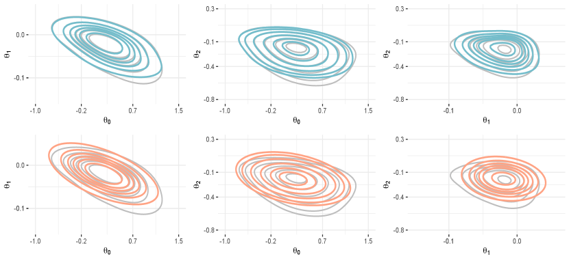
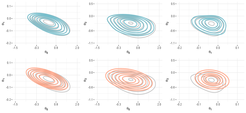
D.4 Probit and logistic regression model from Section 5.2

This section reports some additional results for the real–data analysis described in Section 5.2. Figures D.1 and D.2 strengthen the results within Table 3 in the main article by providing a graphical comparison between the accuracy of the newly–developed skew–modal approximation for the bivariate posteriors in the Cushings dataset, and the one obtained under the classical Gaussian–modal solution. Results confirm again the improved ability of the proposed skew–modal in approximating the target posterior through an accurate characterization of its skewness.

Table D.4: For probit and logistic regression, estimated joint, bivariate and marginal total variation distances between the target posterior and the deterministic approximations under analysis in the Cushings application. The bold values indicate the best performance for each subset of parameters.

$\textsc{tv}_{\theta}$ $\textsc{tv}_{\theta_{01}}$ $\textsc{tv}_{\theta_{02}}$ $\textsc{tv}_{\theta_{12}}$ $\textsc{tv}_{\theta_{0}}$ $\textsc{tv}_{\theta_{1}}$ $\textsc{tv}_{\theta_{2}}$ Probit skew–m $\bf 0.11$ $\bf 0.05$ $\bf 0.06$ $\bf 0.09$ $0.03$ $\bf 0.04$ $\bf 0.05$ gm $0.19$ $0.10$ $0.13$ $0.18$ $0.09$ $0.08$ $0.11$ ep $0.13$ $0.07$ $0.09$ $0.11$ $\bf 0.01$ $0.07$ $0.09$ mf–vb $0.50$ $0.32$ $0.41$ $0.47$ $0.18$ $0.28$ $0.35$ pfm–vb $0.25$ $0.12$ $0.22$ $0.23$ $0.06$ $0.09$ $0.19$ Logit skew–m $\bf 0.14$ $0.08$ $\bf 0.10$ $0.13$ $0.05$ $\bf 0.06$ $\bf 0.07$ gm $0.23$ $0.13$ $0.17$ $0.22$ $0.11$ $0.10$ $0.14$ ep $\bf 0.14$ $\bf 0.07$ $0.11$ $\bf 0.12$ $\bf 0.01$ $0.07$ $0.10$ mf–vb $0.25$ $0.13$ $0.21$ $0.24$ $0.07$ $0.10$ $0.19$

Table D.4 concludes the analysis by assessing the behavior of the newly–proposed skew–m solution when compared against other advanced techniques within the class of deterministic approximations for binary regression models, beyond the classical Gaussian–modal (gm) alternative. State–of–the–art methods under this framework are mean–field variational Bayes (mf–vb) (Consonni and Marin, 2007; Durante and Rigon, 2019) and expectation–propagation (ep) (Chopin and Ridgway, 2017), while partially–factorized variational Bayes (pfm–vb) (Fasano, Durante and Zanella, 2022) is available only for probit regression. mf–vb and pfm–vb for probit regression leverage the implementation in the GitHub repository Probit-PFMVB (Fasano, Durante and Zanella, 2022), while in the logistic setting we rely on the codes in the repository logisticVB (Durante and Rigon, 2019). Note that pfm–vb is designed for probit regression only. Finally, ep is implemented under both models using the code in the GitHub repository GaussianEP.jl by Simon Barthelmé; see also the R library EPGLM (Chopin and Ridgway, 2017) for a previous implementation.

The results in Table D.4 highlight how the use of skew–m ensures noticeable improvements relative to mf–vb and pfm–vb. The advantages over pfm–vb in the probit model are remarkable since also such a strategy leverages a skewed approximation of the target posterior distribution. This yields a higher accuracy than mf–vb, but the improvements are not as noticeable as skew–m. A reason for this result is that pfm–vb has been originally developed to provide high accuracy in high–dimensional $p>n$ settings (Fasano, Durante and Zanella, 2022), whereas in this study $p=3$ and $n=27$ . Remarkably, skew–m yields results competitive also with ep. This fact is noteworthy for at least two reasons. First, Gaussian ep methods are aimed at matching the first two posterior moments. Being global characteristics of the target posterior, these objectives lead to approximations that, albeit symmetric, are often difficult to improve in practice. On the contrary, the proposed skew–m focuses on the local behavior of the posterior distribution in a neighborhood of its mode. It is therefore interesting to notice how inclusion of skewness can dramatically improve the global quality of an approximation, even when targeting its local behavior at the mode. For the Cushing application, this translates into an average for the tv distances in Table D.4 of $0.11$ , lower than the average of $0.14$ achieved by ep. Second, ep techniques typically rely on a convenient factorization of the target density (e.g., Gelman et al., 2013, p. 338). Such a condition is not required for the adoption of skew–m, making it applicable to a wider range of models.

		$\displaystyle\int_{K_{n}}(p_{\theta_{}+h/\sqrt{n}}^{n}/p_{\theta_{}}^{n})(X^{n})\pi(\theta_{}+h/\sqrt{n})/\pi(\theta_{})dh\frac{1}{\mathbbm{1}_{A_{n,4}}}$		(A.7)
		$\displaystyle\quad\geq e^{-\gamma_{1}}\int_{K_{n}}\exp\{-v_{st}^{n}(h-\Delta_{\theta_{}}^{n})_{s}(h-\Delta_{\theta_{}}^{n})_{t}/2\}dh\frac{1}{\mathbbm{1}_{A_{n,4}}}$
		$\displaystyle\quad\quad=\frac{e^{-\gamma_{1}}(2\pi)^{d/2}}{\|V_{\theta_{}}^{n}\|^{1/2}}\int_{K_{n}}\frac{\|V_{\theta_{}}^{n}\|^{1/2}}{(2\pi)^{d/2}}\exp\{-v_{st}^{n}(h-\Delta_{\theta_{}}^{n})_{s}(h-\Delta_{\theta_{}}^{n})_{t}/2\}dh\frac{1}{\mathbbm{1}_{A_{n,4}}}.$

		$\displaystyle\int_{\hat{h}\,:\,\\|\hat{h}\\|<2\sqrt{d}M_{n}}\|2\phi_{d}(\hat{h};0,\hat{\Omega})\hat{w}(\hat{h})-\phi_{d}(\hat{h};0,\hat{\Omega})\|d\hat{h}$		(C.31)
		$\displaystyle\qquad=\int_{\hat{h}\,:\,\\|\hat{h}\\|<2\sqrt{d}M_{n}}\Big{\|}\frac{1}{6\sqrt{n}}\frac{\ell^{(3)}_{\hat{\theta},stl}}{n}\hat{h}_{s}\hat{h}_{t}\hat{h}_{l}+{r}_{F,\delta}\Big{(}\frac{1}{6\sqrt{n}}\frac{\ell^{(3)}_{\hat{\theta},stl}}{n}\hat{h}_{s}\hat{h}_{t}\hat{h}_{l}\Big{)}\Big{\|}\phi_{d}(\hat{h};0,\hat{\Omega})d\hat{h}$
		$\displaystyle\qquad\geq\int_{\hat{h}\,:\,\\|\hat{h}\\|<2\sqrt{d}M_{n}}\Big{\|}\frac{1}{6\sqrt{n}}\frac{\ell^{(3)}_{\hat{\theta},stl}}{n}\hat{h}_{s}\hat{h}_{t}\hat{h}_{l}\Big{\|}\phi_{d}(\hat{h};0,\hat{\Omega})d\hat{h}-\frac{16L_{F,\delta}L_{3}^{2}d^{3}M_{n}^{6}}{9n}.$

Skewed Bernstein–von Mises theorem and skew–modal approximations

Abstract

keywords:

keywords:

1 Introduction

1.1 Notation

2 A skewed Bernstein–von Mises theorem

2.1 Derivation of the skew–symmetric approximating density

2.2 The general theorem

Assumption 1.

Assumption 2.

Assumption 3.

Assumption 4.

Theorem 2.1.

Remark 2.2.

Remark 2.3.

Lemma 2.4.

Proof.

2.3 Skew–symmetric approximations in regular parametric models

Assumption 5.

Assumption 6.

Assumption 7.

Assumption 8.

Corollary 2.5.

Remark 2.6.

Remark 2.7.

2.3.1 Log–posterior asymptotics and posterior contraction

Lemma 2.8.

Lemma 2.9 (Posterior contraction).

2.3.2 Sufficient conditions for Assumption 8

Lemma 2.10.

3 Empirical results

3.1 Exponential model

3.2 Misspecified exponential model

4 Skew–modal approximation

4.1 Skew–modal approximation and theoretical guarantees

Assumption 9.

Assumption 10.

Theorem 4.1.

Remark 4.2.

Remark 4.3.

Remark 4.4.

4.2 Marginal skew–modal approximation and theoretical guarantees

Theorem 4.5.

Remark 4.6.

5 Empirical analysis of skew–modal approximations

5.1 Exponential model revisited

5.2 Probit and logistic regression model

5.3 High–dimensional logistic regression

6 Discussion

References

Appendix A Proofs of Lemmas, Theorems and Corollaries

proof of Lemma 2.4.

proof of Corollary 2.5.

proof of Lemma 2.8.

proof of Lemma 2.9.

proof of Lemma 2.10.

Proof of Theorem 4.5.

Appendix B Technical lemmas

Lemma B.1.

Proof.

Lemma B.2.

Proof.

Lemma B.3.

Proof.

Lemma B.4.

Proof.

Appendix C Non–Asymptotic bounds and proof of Theorem 4.1

Theorem C.1.

Remark C.2.

proof of Theorem C.1.

Lemma C.3.

Proof.

Lemma C.4 (Concentration Gaussian modal approximation).

Proof.

Lemma C.5 (Posterior contraction about map).

proof of Lemma C.5.

Theorem C.6.

Proof.

Appendix D Empirical studies

Skewed Bernstein–von Mises theorem
and skew–modal approximations