Sliding Mode Observers for Set-valued Lur’e Systems with Uncertainties Beyond Observational Range
Abstract
In this paper, we introduce a new sliding mode observer for Lur’e set-valued dynamical systems, particularly addressing challenges posed by uncertainties not within the standard range of observation. Traditionally, most of Luenberger-like observers and sliding mode observer have been designed only for uncertainties in the range of observation. Central to our approach is the treatment of the uncertainty term which we decompose into two components: the first part in the observation subspace and the second part in its complemented subspace. We establish that when the second part converges to zero, an exact sliding mode observer for the system can be obtained. In scenarios where this convergence does not occur, our methodology allows for the estimation of errors between the actual state and the observer state. This leads to a practical interval estimation technique, valuable in situations where part of the uncertainty lies outside the observable range. Finally, we show that our observer is also a - observer as well as a strong observer.
Keywords. Sliding mode observer; set-valued Lur’e systems; uncertainties outside the
observation subspace
AMS Subject Classification. 28B05, 34A36, 34A60, 49J52, 49J53, 93D20
1 Introduction
Differential inclusion serves as an extension of ordinary differential equations, playing a pivotal role as a mathematical model within applied mathematics and control theory. A set-valued Lur’e dynamical system, a form of differential inclusion, incorporates interconnection feedback, broadening its scope to encompass various models frequently used in the analysis of nonsmooth dynamical systems. Such models include evolution variational inequalities, projected dynamical systems, relay systems, and complementarity systems. Set-valued Lur’e dynamical systems have been the subject of thorough investigations in recent decades (we refer, for example, to [1, 2, 3, 7, 8, 9, 12, 14, 20, 22, 27, 28] and the references therein). An observer is a mathematical model used to reconstruct complete information about the state variables from partially measurable data. Observers design for set-valued Lur’e systems represents a significant practical challenge, alongside other fundamental issues like well-posedness and stability analysis, which have received extensive attention in the literature. Numerous references addressing observer design for set-valued Lur’e systems are available, with a predominant focus on two methodological approaches: Luenberger-like techniques [11, 15, 16, 17, 27, 28] and sliding mode methodologies [4, 21].
The Luenberger-like observers for set-valued Lur’e systems was initially explored by Brogliato-Heemels in [11], which is an extension of the work of Arcak-Kokotovic for the nonlinear case [5]. Brogliato-Heemels considered the differential inclusion
| (1) |
and proposed the observer
| (2) |
where are matrices with appropriate dimensions, is a maximal monotone set-valued operator and is the partial measurable output. Later, it was extended by Huang et al in [15] to incorporate uncertainty as follows
| (3) |
where is an unknown constant. The proposed observer is
| (4) |
where the range condition is satisfied for some symmetric positive definite matrix . The key idea in [15] is to approximate the unknown by using an additional ODE, aiming to achieve observer convergence with an unknown rate. On the other hand, B. K. Le [21] proposed a sliding mode observer for a more general class of set-valued Lur’e systems, which extends the nonlinear case considered by Xiang-Su-Chu [29], see also [26] for a survey. Following this, Adly-Le applied the technique to system (3) in [4], offering clear advantages over Luenberger-like methods (4). These advantages include improved assumptions and achieving exponential convergence for the sliding mode observer without the need to solve additional ordinary differential equations. Moreover, the authors proposed a new, efficient smoothing approximation for the sliding mode technique to reduce the chattering effect using time guiding functions.
Nonetheless, a significant limitation of existing results using Luenberger-like or sliding mode observers (we refer, for example, to [4, 15, 21]) is the necessity of the range condition for uncertainties, meaning that uncertainties must fall within the range of . An alternative approach involves constructing observers. However, observers only offer estimations for the entire process under zero initial conditions, rather than providing estimations at specific time instances (see, for instance, [17]). This limitation prompts us to introduce a sliding mode observer to attain time-specific estimations for the Lur’e system in the presence of uncertainties that do not fall within the observation range, as follows:
| (5) |
where are given matrix, is the state variable, is a maximal monotone operator, is the control input and is the measurable output. The nonlinear functions is Lipschitz continuous and is unknown. The model in (5) is quite general since in the right-hand side of the ODE, one has the linear , the nonlinear , the set-valued and the general unknown . The idea is to decompose into 2 parts: where is the projection of onto the observation subspace and is in the complement of the observation subspace. We show that if is bounded, we can obtain a useful estimation for the state of the original system. Interval estimation is practical and unavoidable if the uncertainty is general and not in the range of observation. We refer here some interval observers results for some specific systems [18, 23]. In addition, if tends to vanish when the time is large, we obtain the exact sliding mode observer, i.e., the observer state converges to the original state asymptotically. Finally, we show that our proposed observer is a - observer, a notion that we introduce to obtain a time instant estimation for the error. We also provide a mild additional condition such that our observer is a strong observer, an extension of observers which does not require the zero initial condition. - observers and strong observers allow us to obtain the total process and time instant estimations of the errors. In practice, there is a preference for the insights provided by the characteristics of strong observers over those of observers.
The paper is structured as follows: In Section 2, we revisit established definitions and essential results for our subsequent analyses. Section 3 presents our proposal for a sliding mode observer for the original system, which simultaneously functions as a - observer as well as a strong observer. In Section 4, we give several numerical examples to validate the theoretical findings. The paper concludes in Section 5, where we offer our closing remarks and explore potential future directions.
2 Notations and mathematical background
We denote the scalar product and the corresponding norm of Euclidean spaces by and respectively. A matrix is called positive definite, written , if there exists such that
The Sign functions in is defined by
where denotes the closed unit ball in .
A set-valued mapping is called if for all and , one has
Furthermore, is called if there is no monotone operator such that the graph of is contained strictly in the graph of (see, e.g, [6, 13]).
Let us recall a general version of Gronwall’s inequality [25].
Lemma 1.
Let be given and with for almost all Let the absolutely continuous function satisfy:
| (6) |
where . Then for all :
| (7) |
3 Sliding mode observer and the convergence analysis
In this section, we propose a sliding mode observer for the system (5) under the following assumptions:
Assumption 1: The set-valued operator is a maximal monotone operator.
Assumption 2: The functions is - Lipschitz continuous w.r.t , i.e.:
Assumption 3: There exist , , and such that
| (8) | |||
| (9) |
Assumption 4: The unknown is continuous and can be decomposed as , where is the projection of onto . The terms and are unknown, bounded by known continuous positive functions and respectively, i.e., for all , we have
Remark 1.
i) Assumption 4 is quite general, since it does not require the uncertainty in the range of , i.e., the range of observation.
ii) Suppose that Assumption 4 holds, then we have , i.e., is in the kernel of .
The proposed sliding mode observer for (5) is
| (10) |
where
| (11) |
for some given small . Since the nonlinear and the unknown are continuous, we can obtain the existence and uniqueness of the original system (5) and the approximate observer (10) under some additional mild conditions (see, e.g., [4, 11, 15]). In the following, we show that if is bounded, we obtain a useful estimation for the error . On the other hand, if tends to vanish when the time is large, we have an exact observer indeed.
Theorem 2.
Suppose that Assumptions 1–4 hold. Let Then
| (12) |
where and are the largest and smallest eigenvalues of respectively.
In addition
-
(a)
If is bounded by some , then
(13) Additionally, we introduce the attractive set . Consequently, the error norm converges to any neighborhood of in finite time and remains within that vicinity.
- (b)
-
(c)
If for all , then converges exponentially to zero.
-
(d)
If , then
Proof.
| (14) | |||||
With , one has
| (15) | |||||
From (9) and the monotonicity of , we have
| (16) |
On the other hand, using Assumption 2, we obtain
| (17) |
Thus from (8), (14)-(17), we deduce that
| (18) |
Using Lemma 1 with , we have
(a) If is bounded by some , then
Thus, one obtains . On the other hand, from (18) we have
If for some , one has . Hence classically converges to any neighborhood of in finite time and stay there.
(b) In particular, is bounded by some . Note that from , we imply that
| (19) |
In particular, is bounded and hence is bounded by some . Let be given, and
Then is bounded by and converges to zero since as . Using (19), by replacing by , for all , we obtain
| (20) |
For given , we can choose such that . Then
| (21) |
Thus
Since is arbitrary, we must have
and thus
(c) If for all , then
| (22) | |||||
| (23) |
if .
Thus the error converges to zero with exponential rate. The case is trivial.
Remark 2.
i) In the first case, we have the interval estimation for the error, i.e., the original state belongs to some known interval centered at the approximate observer . In the remaining cases, one obtains the exact observer. It covers the case where the unknown vanishes after some time instant as considered in some examples in [17]. Note that with our observer, we only require that the unknown part in the complement of the observation space tends to vanish (see Figure 3, Example 2).
ii) The term makes small very fast and remains small.
Note that if , then . Thus, if we choose for some and , then
| (25) | |||||
Then decreases very fast in finite time such that .
iii) Suppose that is bounded by , then we can improve the set by the new attractive set .
iv) The same result is obtained if the unknown is replaced by .
Let us recall the definition of observer (see, e.g., [17]) and introduce the notion of strong observer as well as -observer.
Definition 1.
Definition 2.
Definition 3.
Remark 3.
It is easy to see that a strong observer is also an observer while - observer provides a time instant estimation for the error.
Assumption 5: There exists some such that
| (31) |
where and is in Assumption 4.
Theorem 3.
Proof.
From Theorem 2, if the uncertainty , then the error converges to zero exponentially. For non-zero , using Theorem 2-d, we have
| (32) | |||||
which deduces that (10) is a - observer for the system (5). If Assumption 5 is satisfied, from (15)-(17), with the same , we have
| (33) | |||||
Integrating both side from to and note that is non-negative, we obtain that . It means that (10) is a strong observer for the system (5). ∎
Remark 4.
i) Assumption 5 implies that , which is consistent to Assumption 4. In , we use the term instead of as in [17], which is easier to have the non-positiveness of .
ii) The positive number exists, for example, if , we can choose .
4 Numerical examples
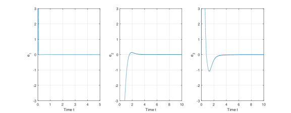
Example 1.
First we consider the system (5) with
Suppose that the unknown and
Then and . Then Assumptions 1–4 are satisfied with
One can observe that the total error converges to any neighborhood of the set in finite time while the observed error tends to zero very fast. Consequently, the observer state using (10) provides a good estimation for the original state .
Example 2.
Next let us consider the rotor system with friction as in [10, 19]. Let , and where and are the angular positions of the upper and lower discs, respectively, we have
| (34) |
where is the input voltage to the power amplifier of the motor, and
| (35) |
Then (34) can be written as
| (36) |
The estimation of the parameters are given in [19, Table 1]. Substituting the values into the functions, we have
We can rewrite (36) as follows
| (37) |
where , , , , . Substituting the estimated values of the parameters, we have
Since is not monotone, we use the loop transformation , where . Then
Under the transformation, we have a new system
| (38) |
where
Here we choose . Solving the following LMIs:
| (39) |
we obtain
Now suppose that the system (38) is influenced by an uncertainty , which is described as follows:
| (40) |
First we take the unknown .
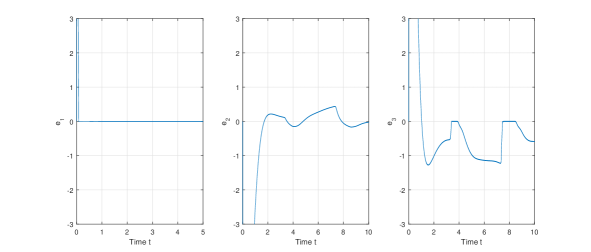
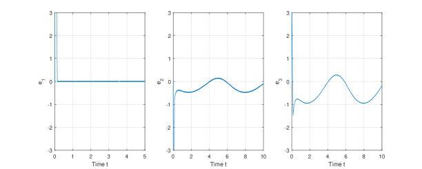
Using the approximate sliding mode observer (10), we can see that observation error converges to zero very fast and the total error module belongs to the attractive set in finite time (Figure 2). The numerical result is consistent with Theorem 2 when the uncertainty is chosen randomly. Next we consider the unknown
which has 2 parts: the first part in and the second part vanishes when the time is large. Then the sliding mode observer (10) is indeed the observer of the original system (Figure 3).
5 Conclusions
In this paper, we introduce a sliding mode observer, which also functions as a - observer and a strong observer, designed for a general category of set-valued Lur’e dynamical systems. Importantly, our approach accommodates scenarios where the uncertainty does not fall within the range of observation. Consequently, we are able to obtain accurate state estimations for the original systems. Furthermore, in cases where the unobservable portion of uncertainty tends to vanish when the time is large, we achieve exact observers. It would be interesting to investigate strategies that enhance the robustness of our proposed observer, enabling it to handle increasingly complex and dynamic uncertainties or disturbances. Exploring ways to incorporate adaptive control strategies into our observer framework would be a promising direction, facilitating its adaptation to evolving system conditions. Optimizing and reducing the size of the attractive set could be a valuable pursuit. The practical application and validation of our observer in real-world systems, such as autonomous vehicles, robotics, or industrial processes, present good opportunities for future exploration. Extending our observer framework to address the challenges posed by set-valued uncertainties would further broaden its applicability and impact. These open questions require further investigation and are beyond the scope of the current paper. They will be the focus of a new research project.
References
- [1] V. Acary, O. Bonnefon, B. Brogliato, Nonsmooth Modeling and Simulation for Switched Circuits, Lecture Notes in Electrical Engineering Vol 69. Springer Netherlands, 2011
- [2] S. Adly, A. Hantoute, B. K. Le, Nonsmooth Lur’e Dynamical Systems in Hilbert Spaces, Set-Valued Var Anal 24(1), 13–35, 2016
- [3] S. Adly, A. Hantoute, B. K. Le, Maximal Monotonicity and Cyclic-Monotonicity Arising in Nonsmooth Lur’e Dynamical Systems”, J Math Anal Appl 448(1), 691–706, 2017
- [4] S. Adly, B. K. Le, Sliding Mode Observer for Set-valued Lur’e Systems and Chattering Removing, Nonlinear Analysis: Hybrid Systems, Vol. 50, November 2023, 101406.
- [5] M. Arcak, P. Kokotovic, Nonlinear observers: A circle criterion design and robustness analysis. Automatica 37, 1923–1930, 2001
- [6] J. Aubin , A. Cellina, Differential Inclusions: Set-valued Maps and Viability Theory. Berlin: Springer Verlag, 1984
- [7] B. Brogliato, Absolute stability and the Lagrange-Dirichlet theorem with monotone multivalued mappings, Syst Control Lett 51 (5), 343–353, 2004
- [8] B. Brogliato, D. Goeleven, Well-posedness, stability and invariance results for a class of multivalued Lur’e dynamical systems, Nonlinear Anal Theory Methods Appl 74, 195–212, 2011
- [9] B. Brogliato, R. Lozano, B. Maschke, O. Egeland, Dissipative Systems Analysis and Control, Springer Nature Switzerland AG, 3rd Edition, 2020
- [10] J. C. A. de Bruin, A. Doris, N. van de Wouw, W. P. M. H. Heemels, H. Nijmeijer, Control of mechanical motion systems with non-collocation of actuation and friction: A Popov criterion approach for input-to-state stability and set-valued nonlinearities, Automatica, Volume 45, Issue 2, 2009, Pages 405–415.
- [11] B. Brogliato, W. P. M. H. Heemels, Observer Design for Lur’e Systems With Multivalued Mappings: A Passivity Approach, IEEE Trans Automat Contr 54(8), 1996–2001, 2009
- [12] B. Brogliato, A. Tanwani, Dynamical Systems Coupled with Monotone Set-Valued Operators: Formalisms, Applications, Well-Posedness, and Stability, SIAM Rev., 62(1), 3–129, 2020
- [13] H. Brezis, Opérateurs Maximaux Monotones et Semi-groupes de Contractions dans les Espaces de Hilbert, Math. Studies 5, North-Holland American Elsevier, 1973
- [14] M. K. Camlibel, J. M. Schumacher, Linear passive systems and maximal monotone mappings, Math Program 157(2), 397–420, 2016
- [15] J. Huang , Z. Han , X. Cai , L. Liu, Adaptive full-order and reduced-order observers for the Lur’e differential inclusion system, Commun Nonlinear Sci Numer Simul 16, 2869–2879, 2011
- [16] J. Huang , Z. Han , X. Cai, Note on observer for Lur’e differential inclusion systems, IET Control Theory & Applications, vol. 5 (17), 2011
- [17] J. Huang, W. Zhang, M. Shi, L. Chen, L. Yu, Observer design for singular one-sided Lur’e differential inclusion system, J Franklin Inst, 3305–3321, 2017
- [18] J. Huang , X. Ma, X. Zhao, H. Che, L. Chen, Interval observer design method for asynchronous switched systems, IET Control Theory & Applications, 2020
- [19] A. L. Juloski, N. Mihajlovic, W. P. M. H. Heemels, N. van de Wouw and H. Nijmeijer, Observer design for an experimental rotor system with discontinuous friction, 2006 American Control Conference, Minneapolis, MN, USA, 2006
- [20] B. K. Le, On a class of Lur’e dynamical systems with state-dependent set-valued feedback, Set-Valued Var Anal 28, 537–557, 2020
- [21] B. K. Le, Sliding Mode Observers for Time-Dependent Set-Valued Lur’e Systems Subject to Uncertainties, J Optim Theory Appl 194, 290–305, 2022
- [22] A.I. Lur’e, V.N. Postnikov. On the theory of stability of control systems. Appl. Math. Mech. 8(3), (1944) (in Russian)
- [23] F. Mazenca, O. Bernard, Interval observers for linear time-invariant systems with disturbances, Automatica 47 (2011) 140–147
- [24] Y. Shtessel, C. Edwards, L. Fridman and A. Levant, Sliding Mode Control and Observation, Birkhauser, 2013
- [25] R. E. Showalter, Monotone Operators in Banach Spaces and Nonlinear Partial Differential Equations, Amer. Math. Society, Providence, RI, 1997
- [26] S. Spurgeon, Sliding mode observers - a survey. Int. J. Syst. Sci. 39(8), 751–764, 2008
- [27] A. Tanwani, B. Brogliato, C. Prieur, Stability and observer design for Lur’e systems with multivalued, non-monotone, time-varying nonlinearities and state jumps, SIAM J. Control Opti., Vol. 52, No. 6, 3639–3672, 2014
- [28] A. Tanwani, B. Brogliato, C. Prieur, Well-Posedness and Output Regulation for Implicit Time-Varying Evolution Variational Inequalities, SIAM J. Control Opti., Vol. 56(2), 751–781, 2018
- [29] J. Xiang, H. Su, J. Chu: On the design of Walcott-Zak sliding mode observer, Proc. Amer. Contr. Conf. Portland, OR, pp. 2451–2456, 2005