The University of Adelaide, Adelaide, Australia
11email: {xiankun.yan,aneta.neumann,frank.neumann}@adelaide.edu.au
Sliding Window Bi-Objective Evolutionary Algorithms for Optimizing Chance-Constrained Monotone Submodular Functions
Abstract
Variants of the GSEMO algorithm using multi-objective formulations have been successfully analyzed and applied to optimize chance-constrained submodular functions. However, due to the effect of the increasing population size of the GSEMO algorithm considered in these studies from the algorithms, the approach becomes ineffective if the number of trade-offs obtained grows quickly during the optimization run. In this paper, we apply the sliding-selection approach introduced in [21] to the optimization of chance-constrained monotone submodular functions. We theoretically analyze the resulting SW-GSEMO algorithm which successfully limits the population size as a key factor that impacts the runtime and show that this allows it to obtain better runtime guarantees than the best ones currently known for the GSEMO. In our experimental study, we compare the performance of the SW-GSEMO to the GSEMO and NSGA-II on the maximum coverage problem under the chance constraint and show that the SW-GSEMO outperforms the other two approaches in most cases. In order to get additional insights into the optimization behavior of SW-GSEMO, we visualize the selection behavior of SW-GSEMO during its optimization process and show it beats other algorithms to obtain the highest quality of solution in variable instances.
Keywords:
chance constraints submodular function evolutionary algorithms runtime analysis.1 Introduction
Evolutionary algorithms (EAs) have been successfully applied to solve a wide range of complex combinatorial optimization problems. The algorithms have received both theoretical and empirical studies, showing their ability to obtain good solutions within a reasonably expected runtime for problems with deterministic settings [3, 7, 8, 11, 19, 26, 31]. Additionally, it has been observed that some EAs also perform effectively on stochastic and dynamic optimization problems. Researchers are actively investigating the advantages and limitations of EAs in solving such problems, particularly within the field of evolutionary computation theory. A variety of studies [12, 14, 20, 18, 27, 29, 32] have been conducted, presenting both the challenges and the advanced implications of these algorithms.
In a stochastic environment, completely eliminating the negative and uncertain impact of stochastic components is challenging. Therefore, it is crucial to minimize these negative effects to prevent unpredictable disruptions in most complex systems. Chance constraint [1, 5, 9, 15, 22, 23, 24, 25] is a useful technique for handling the effects of stochastic circumstances. It allows the deterministic bound in the constraint to be violated, but only with a very small probability during optimization. However, directly evaluating chance constraints is complex and time-consuming. A practical approach is to transform the stochastic constraint into its corresponding deterministic equivalent for a given confidence level, rather than statistically calculating the probability of violation when optimizing chance-constrained problems with known distribution elements [30, 32].
Submodular functions [16] represent various problems where the incremental benefit of adding solution elements diminishes with the increasing solution size. The optimization of submodular functions is significantly challenging and has been extensively investigated with different types of constraints in previous work [10, 13, 16, 21, 27, 33, 34]. In the paper, we study a chance-constrained version of the submodular optimization problem subject to a knapsack constraint. The problem seeks to find a subset of stochastic elements that maximizes the submodular function value, while ensuring that the actual weight exceeds a given bound with a very small probability. In the previous research, Doerr et al [4] analyzed the performance of the greedy algorithms on the problem. They constructed the surrogate functions using the tail inequalities (Chernoff bound and one-sided side Chebyshev’s inequality) to handle the chance constraint. Their findings demonstrated the greedy algorithms can achieve -approximation and -approximation for the problem with the uniform independent and identically distributed (IID) weights and the uniform weights with the same dispersion respectively. Subsequently, Neumann et al., [17] applied the Global Simple Evolutionary Multi-objective Algorithm (GSEMO) to the same problem. They employed a similar surrogate approach for estimating violation probability as done in [4] and considered both the submodular function value and the probability as objectives in their bi-objective fitness function. Their theoretical analysis demonstrated that the GSEMO can achieve similar approximation results as [17] within an expected runtime related to the max population size that it can generate. Additionally, their experimental results indicated that the GSEMO could obtain better solutions than the greedy algorithm and other evolutionary algorithms, in solving the problem involving uniform IID weights.
However, the runtime analysis presented in [17] indicates that the growing population size significantly impacts the efficiency of the GSEMO. This is particularly evident when dealing with uniform weights of the same dispersion, where the GSEMO can quickly maintain an exponential number of trade-off solutions in the population. To address this inefficiency, the sliding-selection approach has been introduced, leading to the development of an improved version of GSEMO, named the Sliding Window GSEMO (SW-GSEMO). Neumann and Witt [21] firstly presented the SW-GSEMO’s enhanced performance in solving submodular problems with deterministic weights. In brief, the sliding-selection method involves defining a weight window of size one, which is determined based on the given bound and the ratio of the current time to the total time. A solution is eligible for selection as a parent if its weight falls within the current window; otherwise, the algorithm uniformly selects one individual from the current population.
Within this paper, the SW-GSEMO is slightly updated in terms of the window selection method for optimizing chance-constrained monotone submodular functions. The individuals that are in the window are still potential parents for the mutation, however, when there is no individual in the window area, the algorithm chooses a current solution with the largest function value as the parent for the next mutation unless the current time exceeds the time budget. Following the approach in [17], the fitness function in our algorithm contains two objectives: the evaluated weight and the function value of the solution. We also employ the same surrogate methods based on tail inequalities for weight evaluation. Our study includes settings that include both IID weights, and uniform weights with the same dispersion. Our analysis reveals that the incorporation of the sliding-selection approach reduces the impact of growing population size on the expected runtime. As a result, the expected runtime of the SW-GSEMO to achieve similar expected approximation results shows improvement. Additionally, we empirically assess the performance of the SW-GSEMO on the maximum coverage problem under various settings, bounds, and violation probabilities. We compare its results with those from the original GSEMO and the Non-Dominated Sorting Genetic Algorithm II (NSGA-II ). The initial solutions of all algorithms are empty sets and the NSGA-II uses population sizes of and respectively. Furthermore, we provide a visualization of the sliding window’s operation during optimization. Our investigation also seeks why algorithms using surrogates based on the Chernoff bound perform better than those using the one-sided Chebyshev’s inequality when the probability is smaller.
The paper is structured as follows. Section 2 introduces the chance-constrained monotone submodular problem and the investigated settings. Section 3 describes the adopted multi-objective evolutionary algorithms. Our theoretical runtime analysis and proofs of the SW-GSEMO are presented in Section 4. Then we investigate the performance of the different algorithms and visualize the selection behavior in Section 5. Finally, we end with some conclusions in Section 6.
2 Preliminaries
Given a set , we consider the optimization of a monotone submodular function . A function is called monotone iff for every with , holds. A function is called submodular iff for every with , and , holds. We consider the optimization of such a function subjected to the chance constraint where each element takes on a random weight . Here, the chance-constrained optimization problem can be formulated as
where is the total weight of the subset , and is the given deterministic bound. The parameter quantifies the probability of exceeding the bound that can be tolerated.
Following previous work [4, 17], we consider two different settings, which are (1) Uniform IID Weights: the weight of each element is sampled from the uniform distribution with the same expected value and dispersion (i.e., ] and ); and (2) Uniform Weights with the Same Dispersion: the weight of element is sampled from the uniform distribution with the different expected value but the same dispersion (i.e., and ). In both settings, we assume that the expected weight of each element is a positive integer. For further discussion, the subset is encoded as a decision vector with length , where means that the element is selected into the subset . Besides, we denote the number of elements packed into the subset . Since all the settings are based on the uniform distribution, we have the expected weight and variance of the solution as
and
To handle the chance constraint, we establish the surrogate function based on One Chebyshev’s inequality and Chernoff bound as described in the previous work [4, 17]. The weight calculated by different surrogate functions are respectively formulated as
and
It had been proved that if the surrogate weight of a solution is less than the bound , then is feasible [4].
3 Multi-Objective Evolutionary Algorithm
Input: Probability , bound
Output: the best individual
Input: Total time , probability , bound
Output: the best individual
Input: Population P, current iteration , total time , probability , bound
Output: the selected individual
Within the paper, we primarily investigate multi-objective evolutionary algorithms on the given monotone submodular problem. Each solution is considered to be a two-dimensional search point in the objective space. The bi-objective fitness function of the solution is expressed as
| (1) |
| (2) |
where denotes the submodular function value of , denotes the surrogate weight of . Let be another solution in the search space. We say that (weakly) dominates iff and . Note that the infeasible solution is strongly dominated by the feasible one because of the objective function . Besides, the objective function guides the generated solutions approach to the feasible search space.
In previous work [17], the GSEMO (see Algorithm 1) is studied on the chance-constrained monotone submodular problem. Here the GSEMO starts with an initial solution represented by a bitstring, signifying an empty set. During the optimization, it maintains a set of non-dominated solutions, continually updating this set as new solutions are generated. In each iteration, the GSEMO randomly and uniformly selects an individual from the population to serve as a parent for creating offspring via a standard bit-flip operator, which flips each bit of independently with a probability of . The offspring is accepted into the population if it is not strictly dominated by any existing solution. Subsequently, any solution in the population that is weakly dominated by is removed.
The modified SW-GSEMO algorithm is outlined in Algorithm 2. It also begins with a bitstring, maintains a population of non-dominating individuals, and employs the standard mutation to generate offspring. However, it differs from the GSEMO in its parent selection method, which defines a sliding window (see Algorithm 3) to select the potential parents instead of applying the random uniform selection in the whole population directly. Within this method, given the total runtime and the current time , a current bound is defined as . A window is established as an interval between . Unlike the deterministic case where it selects solutions based on deterministic weight, the SW-GSEMO chooses some eligible individuals whose surrogate weights fall within this window. The parent is then randomly selected from these eligible solutions. As the current time increases, the SW-GSEMO would select solutions with larger surrogate weights that are still within the window. When no individual lies within the current window, the SW-GSEMO generates a sub-population where the solution from the original population has the surrogate weight that is lower than . Then the solution with the largest -value is assigned for the mutation. Moreover, when , the SW-GSEMO reverts to selecting parents from the entire population , similar to the GSEMO.
4 Performance of SW-GSEMO based on Surrogate
To illustrate that the SW-GSEMO works more efficiently in optimizing the chance-constrained monotone submodular problem than the GSEMO, the expected runtime of SW-GSEMO with the surrogates to reach the same expected result for the problem is analyzed in this section.
4.1 Uniform IID Weights
The previous work [17] illustrates that the classical GSEMO reaches a -approximation for the chance-constrained problem with uniform IID weights in the expected time , where . However, with the help of the sliding-selection, the size of the potential parents is bounded, so the time to get a result with the same approximation is optimized.
Theorem 4.1
Consider SW-GSEMO with on a monotone submodular function under a chance constraint with uniform IID weights. Then with probability , the time that the algorithm finds a solution is no worse than -approximation is bounded by if .
Proof
Let . As far as the previous work [17] proved, the initial bitstring will stay in the population since it is the best individual with respect to . Besides, note that is a strictly monotonically increasing function with the number of elements, and solutions with the same number of elements have the same -value because of the IID weights. From [17], it says that the element with the largest marginal gain to the solution is picked up in the mutation with the probability , the solution that includes the largest elements is kept in population and satisfies the chance constraint, and holds
Note that because of the chance constraint.
We denote a subset of with first elements (i.e., and ). First, we consider how the SW-GSEMO includes the element when the solution is not dominated by other solutions from the population. Recall that the solution with an empty set is kept in the population already at the beginning. Besides, the surrogate weight of is increasing with respect to . We assume that the solution is in the population at time . By definition of , is available for the selection up to time
since
Furthermore, since and , the size of is at most 1 with the effect from the dispersion . Consequently, the probability of choosing the subset and mutating the element is at least between the time and , i.e., for a period of steps, the probability of those events not processing is at most
Then, we study the case where the solution is dominated by an individual solution with a larger -value from the population. That also means is not in the current window at time . We denote as the solution if it exists in the current window. Regarding the domination scheme of the algorithm, it implies that and . Considering the Line 6 of sliding-selection in Algorithm 3, the SW-GSEMO uses the solution (or when no individual is in the current window) for the next mutation. With the probability of at least , the element can be added to the selected solution within the same time period. Consequently, the failure probability is also at most . Besides, the feasible offspring still satisfies .
By a union bound over the at most required successes, the probability of missing including to the solution in the period by time is . Then following [17], applying the surrogate for bounding the value of can get -approximation. ∎
4.2 Uniform Weights with the Same Dispersion
Following the definition from [17], we use the objective function instead of and the already mentioned objective function in the two-dimensional fitness function. Thus, the fitness of a solution is evaluated by . Consequently, it has another solution such that is (weakly) dominated by iff and . Note that will be also used in Algorithm 3.
Additionally, let , , and . Then we show that the SW-GSEMO can get a result with -approximation in an efficient runtime if the solution has at least one element (i.e., ) in the following theorem.
Theorem 4.2
Let be the maximal size of the population. Consider SW-GSEMO with on a monotone submodular function under a chance constraint with uniform weights having the same dispersion. Then with probability , a solution that is no worse than -approximation is obtained within time .
Proof
Following the proof of theorem 2 in [17], we also adopt , the maximal -value for which , to track the progress of the SW-GSEMO. Recall that the bitstring exists in the population at the beginning and is non-decreasing. Considering a chosen solution for mutation, the algorithm flips a 0-bit of corresponding to the largest ratio between the additional gain in and . After mutation, the generated solution holds
where and is the deterministic optimal solution for the problem with the deterministic uniform weight setting. Note that increase by at least .
First, we consider such solution is not dominated by any solution in the current population. We prove that the solution is chosen and such mutation in happens with a high probability in the SW-GSEMO. Note that the is growing with respect to its size of elements . By the definition of the subset , such mutation happens in the time between to , since
Thus, the available period is . Since , the size of consequently is bound by as (recall the setting where all the expected weighs are positive integers). Then we have such one bit of flipping that occurs with a probability of at least . Furthermore, the probability of the mutation that does not happen in the period is bounded by
Now we investigate the case when there is a solution dominates the solution . That means does not exist in the current window at the time . Recall that there are at most two individuals in the current window. We denote them by and , which are satisfies and (or ). Regarding the sliding selection, Both solutions and (or when no individual is in the current window) are good to be selected for the mutation since their function values are larger than the value of solution . Therefore, such a 1-bit flipping to get a qualified solution is under the probability . Within the same period, the probability of failure is bounded by .
By a union bound over at most required successes, the probability of failing to achieve at least one success is at most . Therefore, the solution can be obtained in the SW-GSEMO with the probability of at least .
Let be the feasible solution with in the population, which has the largest surrogate weights. Here we consider the single element having the largest -value but not included in . Following the work [17], the algorithm can obtain a solution that only contains from the initial solution by flipping only one zero bit in the expected time , where is the maximal size of population for the algorithm. Then after applying the surrogate for bounding the value of as desired in [17], the quality of or is . Finally, the expected time of SW-GSEMO to get the expected result is . ∎
Backing into the special case of uniform IID weights, we note that , the size of the population is at most , and the solution already contains the element with the largest -value. Besides, as the effect of the uncertainty, the window only includes at most 1 solution. Therefore, gives a - approximation and the expected time to get is bounded by , which matches the result proved in Theorem 4.1.
5 Experiments
The experimental investigations of the SW-GSEMO based on the different surrogate functions are proposed here. The results are compared with those generated from the GSEMO and the NSGA-II in various instances.
5.1 Experimental setup
The maximum coverage problem (MCP) based on the graph [6, 10] is studied in the experiments, which is one of the famous submodular combinatorial optimization problems. For the MCP, given an undirected graph with nodes, we denote the number of all nodes of and their neighbors in the graph . The goal of the problem is to find a subset of nodes so that the nodes in the subset can cover more to their neighbors and themselves under the chance constraint with a deterministic bound . Also, each node has a stochastic weight . Therefore, the chance-constrained version of the problem is formulated as
| (3) |
Here some larger sparse graphs from the network data repository [28] are considered to construct the instance of MCP. The previous works [17] studied the performance of GSEMO on the problem based on some small and dense graphs and showed it can easily cover most nodes even given a small bound. Thus, utilizing the larger sparse graphs can help us easily compare the results between the different algorithms. Those graphs ca-CSphd, ca-GrQc, and ca-ConMat are applied, which respectively contain , , and nodes.
For the experiments under uniform IID weights, each node is assigned a unit expected weight (i.e., ) and the dispersion Additionally, for the experiments considering uniform weights with the same dispersion, the expected weight of each node is based on its degree, which is expressed as where is the degree of in graph . For the dispersion, we set to ensure . Besides, we employ to ensure that the bounds are proportional to the number of nodes in the graphs under study.
For all experiments, the problem is tested with . In terms of the GSEMO and the SW-GSEMO, the total iterations (or total time) are considered different as Regarding the NSGA-II , the initial solutions are set to the strings. Its population sizes are set as and with the numbers of generated children and respectively. Thus, to keep the same fitness evaluation counts as other algorithms, the max iterations for the NSGA-II are and respectively. Moreover, we adopt the Kruskal-Wallis test with 95% confidence in order to assess the statistical validity of our results. The Bonferroni post-hoc statistical procedure is employed for multiple comparisons of a control algorithm [2]. For the given instance, is equivalent to the statement that the algorithm in the column is statistically better than the algorithm for the tested instance. Conversely, is equivalent to the statement that outperformed the algorithm, while demonstrates that the algorithm given in the column and have a comparable performance.
| GSEMO with (1) | SW-GSEMO with (2) | with (3) | with (4) | |||||||||||||
|---|---|---|---|---|---|---|---|---|---|---|---|---|---|---|---|---|
| Graph | Surrogate | Mean | std | stat | Mean | std | stat | Mean | std | stat | Mean | std | stat | |||
| ca-CondaMat | Chebyshev | 146 | 1500000 | 0.1 | 5588 | 47.265 | 2(-),3(+),4(-) | 6790.966 | 12.335 | 1(+),3(+),4(+) | 5187.966 | 95.708 | 1(-),2(-),4(-) | 6330.3 | 36.893 | 1(+),2(-),3(+) |
| 0.001 | 4153.733 | 43.338 | 2(-),3(+),4(-) | 4748.166 | 7.585 | 1(+),3(+),4(+) | 3802.733 | 75.95 | 1(-),2(-),4(-) | 4531.83 | 33.061 | 1(+),2(-),3(+) | ||||
| 1000000 | 0.1 | 5500.73 | 47.67 | 2(-),3(+),4(-) | 6771.366 | 16.3 | 1(+),3(+),4(+) | 4945.9 | 113.293 | 1(-),2(-),4(-) | 6281 | 46.322 | 1(+),2(-),3(+) | |||
| 0.001 | 3957.5 | 40.782 | 2(-),3(+),4(-) | 4736.133 | 10.375 | 1(+),3(+),4(+) | 3709.06 | 96.656 | 1(-),2(-),4(-) | 4496.7 | 28.765 | 1(+),2(-),3(+) | ||||
| 500000 | 0.1 | 4818.53 | 47.71 | 2(-),3(+),4(-) | 6708.366 | 27.316 | 1(+),3(+),4(+) | 4685.333 | 114.8373 | 1(-),2(-),4(-) | 6115.233 | 54.393 | 1(+),2(-),3(+) | |||
| 0.001 | 3648.3 | 65.33 | 2(-),3(+),4(-) | 4581.633 | 36.88 | 1(+),3(+),4(+) | 3469.766 | 73.953 | 1(-),2(-),4(-) | 4395.566 | 43.076 | 1(+),2(-),3(+) | ||||
| 1068 | 1500000 | 0.1 | 11787.533 | 57.133 | 2(-),3(+),4(-) | 16650.933 | 14.163 | 1(+),3(+),4(+) | 12284.866 | 142.248 | 1(-),2(-),4(-) | 13394.133 | 75.448 | 1(+),2(-),3(+) | ||
| 0.001 | 10893.9 | 61.683 | 2(-),3(+),4(-) | 15217.3 | 14.45 | 1(+),3(+),4(+) | 10950.3 | 122.3 | 1(-),2(-),4(-) | 12241.966 | 72.716 | 1(+),2(-),3(+) | ||||
| 1000000 | 0.1 | 11194.23 | 72.488 | 2(-),3(-),4(-) | 16573.6 | 19.608 | 1(+),3(+),4(+) | 11623.93 | 119.467 | 1(+),2(-),4(-) | 13164.2 | 60.07 | 1(+),2(-),3(+) | |||
| 0.001 | 10364.53 | 58.95 | 2(-),3(+),4(-) | 15145.666 | 14.485 | 1(+),3(+),4(+) | 9987.13 | 123.936 | 1(-),2(-),4(-) | 12040.166 | 99.78 | 1(+),2(-),3(+) | ||||
| 500000 | 0.1 | 9474.733 | 111.851 | 2(-),3(-),4(-) | 16368.6 | 27.005 | 1(+),3(+),4(+) | 10729.133 | 180.573 | 1(+),2(-),4(-) | 12708.533 | 82.447 | 1(+),2(-),3(+) | |||
| 0.001 | 9344.733 | 84.931 | 2(-),3(-),4(-) | 14947.6 | 22.553 | 1(+),3(+),4(+) | 9502.2 | 142.003 | 1(+),2(-),4(-) | 11581.066 | 84.55 | 1(+),2(-),3(+) | ||||
| 2136 | 1500000 | 0.1 | 12749.533 | 93.378 | 2(-),3(-),4(-) | 20078.833 | 11.066 | 1(+),3(+),4(+) | 16361.766 | 67.76 | 1(+),2(-),4(-) | 16243.166 | 68.601 | 1(+),2(-),3(+) | ||
| 0.001 | 12730.3 | 91.025 | 2(-),3(-),4(-) | 19327.433 | 11.221 | 1(+),3(+),4(+) | 15224.733 | 66.313 | 1(+),2(-),4(-) | 15402.133 | 96.35 | 1(+),2(-),3(+) | ||||
| 1000000 | 0.1 | 11520.966 | 129.843 | 2(-),3(-),4(-) | 20016.2 | 16.172 | 1(+),3(+),4(+) | 15696.5 | 116.216 | 1(+),2(-),4(-) | 16020.633 | 88.739 | 1(+),2(-),3(+) | |||
| 0.001 | 11500.633 | 114.875 | 2(-),3(-),4(-) | 19245.233 | 15.532 | 1(+),3(+),4(+) | 14544.63 | 98.014 | 1(+),2(-),4(-) | 15155.4 | 74.248 | 1(+),2(-),3(+) | ||||
| 500000 | 0.1 | 9488.333 | 90.631 | 2(-),3(-),4(-) | 19822.566 | 20.619 | 1(+),3(+),4(+) | 14592.466 | 104.587 | 1(+),2(-),4(-) | 14734.2 | 230.948 | 1(+),2(-),3(+) | |||
| 0.001 | 9483.6 | 88.03 | 2(-),3(-),4(-) | 19030.533 | 21.451 | 1(+),3(+),4(+) | 13456.133 | 89.165 | 1(+),2(-),4(-) | 14399.233 | 152.192 | 1(+),2(-),3(+) | ||||
| ca-CondaMat | Chernoff | 146 | 1500000 | 0.1 | 5321.1333 | 40.291 | 2(-),3(+),4(-) | 6424.2 | 10.403 | 1(+),3(+),4(+) | 4931.833 | 82.145 | 1(-),2(-),4(-) | 6018.066 | 41.946 | 1(+),2(-),3(+) |
| 0.001 | 5027.166 | 49.31 | 2(-),3(+),4(-) | 5994.833 | 10.96 | 1(+),3(+),4(+) | 4622.866 | 96.07 | 1(-),2(-),4(-) | 5652.833 | 41.121 | 1(+),2(-),3(+) | ||||
| 1000000 | 0.1 | 5059.6 | 39.678 | 2(-),3(+),4(-) | 6397.966 | 14.943 | 1(+),3(+),4(+) | 4755.133 | 73.411 | 1(-),2(-),4(-) | 5954.966 | 50.251 | 1(+),2(-),3(+) | |||
| 0.001 | 4784.766 | 54.93 | 2(-),3(+),4(-) | 5979.9 | 16.912 | 1(+),3(+),4(+) | 4441.5 | 126.327 | 1(-),2(-),4(-) | 5582.666 | 38.694 | 1(+),2(-),3(+) | ||||
| 500000 | 0.1 | 4625.4 | 60.563 | 2(-),3(+),4(-) | 6328.2 | 31.971 | 1(+),3(+),4(+) | 4443.2 | 84.517 | 1(-),2(-),4(-) | 5787.266 | 63.911 | 1(+),2(-),3(+) | |||
| 0.001 | 4344.33 | 59.972 | 2(-),3(+),4(-) | 5898.133 | 22.47 | 1(+),3(+),4(+) | 4170 | 103.826 | 1(-),2(-),4(-) | 5437.7 | 43.076 | 1(+),2(-),3(+) | ||||
| 1068 | 1500000 | 0.1 | 11632.833 | 52.573 | 2(-),3(-),4(-) | 16650.933 | 14.163 | 1(+),3(+),4(+) | 12054.233 | 126.656 | 1(+),2(-),4(-) | 13206.26 | 65.605 | 1(+),2(-),3(+) | ||
| 0.001 | 11464.966 | 61.738 | 2(-),3(-),4(-) | 15217.3 | 14.45 | 1(+),3(+),4(+) | 11783.9 | 95.969 | 1(+),2(-),4(-) | 12974.86 | 85.587 | 1(+),2(-),3(+) | ||||
| 1000000 | 0.1 | 11059.2 | 73.482 | 2(-),3(-),4(-) | 16343.833 | 16.806 | 1(+),3(+),4(+) | 11441.2 | 145.704 | 1(+),2(-),4(-) | 12961.266 | 85.324 | 1(+),2(-),3(+) | |||
| 0.001 | 10914.833 | 76.11 | 2(-),3(-),4(-) | 16052.866 | 19.687 | 1(+),3(+),4(+) | 11208.1 | 91.525 | 1(+),2(-),4(-) | 12779.033 | 59.812 | 1(+),2(-),3(+) | ||||
| 500000 | 0.1 | 9482.966 | 92.698 | 2(-),3(-),4(-) | 16129.133 | 27.284 | 1(+),3(+),4(+) | 10487.566 | 128.411 | 1(+),2(-),4(-) | 12489.3 | 88.034 | 1(+),2(-),3(+) | |||
| 0.001 | 9466.433 | 113.403 | 2(-),3(-),4(-) | 15840.433 | 26.94 | 1(+),3(+),4(+) | 10254.133 | 130.19 | 1(+),2(-),4(-) | 12309.4 | 81.884 | 1(+),2(-),3(+) | ||||
| 2136 | 1500000 | 0.1 | 12719.533 | 106.011 | 2(-),3(-),4(-) | 19955.3 | 10.312 | 1(+),3(+),4(+) | 16187.466 | 93.583 | 1(+),2(-),4(-) | 16130.1 | 80.711 | 1(+),2(-),3(+) | ||
| 0.001 | 12701.7 | 90.339 | 2(-),3(-),4(-) | 19813.8 | 14.041 | 1(+),3(+),4(+) | 16006.8 | 109.226 | 1(+),2(-),4(-) | 15964.933 | 75.003 | 1(+),2(-),3(+) | ||||
| 1000000 | 0.1 | 11481.066 | 98.619 | 2(-),3(-),4(-) | 19891.466 | 13.197 | 1(+),3(+),4(+) | 15519.3 | 102.403 | 1(+),2(-),4(-) | 15812.433 | 93.623 | 1(+),2(-),3(+) | |||
| 0.001 | 11458.1 | 116.396 | 2(-),3(-),4(-) | 19750.366 | 12.084 | 1(+),3(+),4(+) | 15323.266 | 103.988 | 1(+),2(-),4(-) | 15684.533 | 83.137 | 1(+),2(-),3(+) | ||||
| 500000 | 0.1 | 9451.033 | 105.529 | 2(-),3(-),4(-) | 19697.033 | 17.995 | 1(+),3(+),4(+) | 14435.233 | 101.01 | 1(+),2(-),4(-) | 14650.033 | 289.611 | 1(+),2(-),3(+) | |||
| 0.001 | 9460.666 | 116.783 | 2(-),3(-),4(-) | 19540.266 | 18.77 | 1(+),3(+),4(+) | 14218.8 | 129.106 | 1(+),2(-),4(-) | 14586.566 | 214.181 | 1(+),2(-),3(+) | ||||
5.2 Experimental results
In the experiments, we first investigate the performance of SW-GSEMO on the problem with different settings. Then, we visualize and demonstrate the behavior of the sliding-selection approach working in the optimization.
5.2.1 Results comparison
Table 1 and 2 displays the final function values achieved by the algorithms in the problem with different settings, which vary based on the surrogate functions used, and are tested across different iterations and values of . Additional results are provided in Tables 4, 5, 6 and 7 in Appendix111Appendix is in here.. Overall, for smaller graphs with a lower bound , the SW-GSEMO, GSEMO, and NSGA-II with different population sizes perform comparably. However, the NSGA-II can get better results when the expected weights are uniform, which is reflected in Table 2. For larger graph instances with larger bounds, the SW-GSEMO gradually surpasses the other algorithms in performance. The mean and standard deviation of the SW-GSEMO’s results are also comparable to those of other algorithms across instances with varying . It is observed that as increases, the general performance of all algorithms improves. Moreover, while the function value differences for various are not significant in larger graphs with higher bounds, they become substantial in smaller graphs. Interestingly, the performance of the NSGA-II with population sizes of 20 and 100 is superior to that of the GSEMO in larger, sparser graph cases. This observation contrasts with findings from previous work [17], which uses dense graphs. In terms of evaluating the problem with chance constraints by different surrogate methods, the results from Table 1 and 2 suggest that algorithms employing the one-sided Chebyshev’s inequality are better than those using the Chernoff bound when is large. On the other hand, the performance of algorithms based on the Chernoff bound becomes worse with smaller values.
| GSEMO (9) | SW-GSEMO (10) | (11) | (12) | |||||||||||||
| Graph | Surrogate | Mean | std | stat | Mean | std | stat | Mean | std | stat | Mean | std | stat | |||
| ca-CondaMat | Chebyshev | 146 | 1500000 | 0.1 | 141.266 | 0.679 | 10(=),11(=),12(=) | 141.8 | 0.979 | 9(=),11(=),12(=) | 141.266 | 0.813 | 9(=),10(=),12(=) | 141.8 | 0.979 | 9(=),10(=),11(=) |
| 0.001 | 122.9 | 3.014 | 10(-),11(-),12(-) | 125.933 | 0.249 | 9(+),11(=),12(=) | 125.7 | 0.458 | 9(+),10(=),12(=) | 126 | 0 | 9(+),10(=),11(=) | ||||
| 1000000 | 0.1 | 141.2 | 0.6 | 10(=),11(=),12(=) | 141.733 | 0.963 | 9(=),11(=),12(=) | 141 | 0.632 | 9(=),10(=),12(=) | 141.533 | 0.884 | 9(=),10(=),11(=) | |||
| 0.001 | 122.23 | 3.051 | 10(-),11(-),12(-) | 125.9 | 0.3 | 9(+),11(=),12(=) | 125.366 | 1.048 | 9(+),10(=),12(=) | 126 | 0 | 9(+),10(=),11(=) | ||||
| 500000 | 0.1 | 141.133 | 0.498 | 10(=),11(=),12(=) | 141.8 | 0.979 | 9(=),11(=),12(=) | 140.833 | 0.734 | 9(=),10(=),12(=) | 141.333 | 0.745 | 9(=),10(=),11(=) | |||
| 0.001 | 120.733 | 3.172 | 10(-),11(-),12(-) | 125.6 | 0.663 | 9(+),11(=),12(=) | 124.066 | 2.657 | 9(+),10(=),12(=) | 125.7 | 0.458 | 9(+),10(=),11(=) | ||||
| 1068 | 1500000 | 0.1 | 1037.266 | 1.093 | 10(-),11(+),12(=) | 1044.833 | 0.933 | 9(+),11(+),12(+) | 1015.333 | 4.706 | 9(-),10(-),12(-) | 1037.833 | 2.646 | 9(=),10(-),12(+) | ||
| 0.001 | 978.4 | 2.751 | 10(-),11(+),12(-) | 991.766 | 2.347 | 9(+),11(+),12(=) | 959.566 | 10.892 | 9(-),10(-),12(-) | 992.2 | 3.664 | 9(+),10(=),11(+) | ||||
| 1000000 | 0.1 | 1034.933 | 1.152 | 10(-),11(+),12(=) | 1044.133 | 1.231 | 9(+),11(+),12(+) | 1012.333 | 5.204 | 9(-),10(-),12(-) | 1036.833 | 2.956 | 9(=),10(-),12(+) | |||
| 0.001 | 975.1 | 2.3288 | 10(-),11(+),12(-) | 989.5 | 2.202 | 9(+),11(+),12(=) | 954.866 | 10.616 | 9(-),10(-),12(-) | 991.3 | 3.377 | 9(+),10(=),11(+) | ||||
| 500000 | 0.1 | 1030.833 | 1.293 | 10(-),11(+),12(+) | 1041.633 | 1.251 | 9(+),11(+),12(+) | 1008.633 | 6.441 | 9(-),10(-),12(-) | 1035.233 | 2.641 | 9(+),10(-),12(+) | |||
| 0.001 | 967.666 | 3.418 | 10(-),11(+),12(-) | 985.9 | 2.748 | 9(+),11(+),12(=) | 947.233 | 10.932 | 9(-),10(-),12(-) | 988.866 | 4.145 | 9(+),10(=),11(+) | ||||
| 2136 | 1500000 | 0.1 | 2035.066 | 2.92 | 10(-),11(+),12(+) | 2071.066 | 1.412 | 9(+),11(+),12(+) | 1963.4 | 9.844 | 9(-),10(-),12(-) | 2025.6 | 5.689 | 9(+),10(-),11(+) | ||
| 0.001 | 1925.3 | 3.671 | 10(-),11(+),12(-) | 1972.433 | 3.402 | 9(+),11(+),12(+) | 1850.633 | 13.345 | 9(-),10(-),12(-) | 1942.566 | 6.189 | 9(+),10(-),11(+) | ||||
| 1000000 | 0.1 | 2026.966 | 3.341 | 10(-),11(+),12(+) | 2068.033 | 1.905 | 9(+),11(+),12(+) | 1956.3 | 9.987 | 9(-),10(-),12(-) | 2022.6 | 6.58 | 9(+),10(-),11(+) | |||
| 0.001 | 1914.7 | 3.831 | 10(-),11(+),12(-) | 1969.433 | 3.666 | 9(+),11(+),12(+) | 1839.766 | 13.313 | 9(-),10(-),12(-) | 1939.833 | 7.55 | 9(+),10(-),11(+) | ||||
| 500000 | 0.1 | 2009.366 | 4.214 | 10(-),11(+),12(-) | 2063.166 | 2.852 | 9(+),11(+),12(+) | 1941.3 | 11.346 | 9(-),10(-),12(-) | 2016.5 | 5.942 | 9(+),10(-),11(+) | |||
| 0.001 | 1893.5 | 4.055 | 10(-),11(+),12(-) | 1960 | 3.705 | 9(+),11(+),12(+) | 1821 | 14.61 | 9(-),10(-),12(-) | 1931.866 | 6.443 | 9(+),10(-),11(+) | ||||
| ca-CondaMat | Chernoff | 146 | 1500000 | 0.1 | 139 | 0 | 10(=),11(=),12(=) | 139 | 0 | 9(=),11(=),12(=) | 139 | 0 | 9(=),10(=),12(=) | 139 | 0 | 9(=),10(=),11(=) |
| 0.001 | 137.1 | 1.445 | 10(=),11(=),12(=) | 138.2 | 1.326 | 9(=),11(=),12(=) | 136.9 | 1.374 | 9(=),10(=),12(=) | 138.3 | 1.268 | 9(=),10(=),11(=) | ||||
| 1000000 | 0.1 | 139 | 0 | 10(=),11(=),12(=) | 139 | 0 | 9(=),11(=),12(=) | 139 | 0 | 9(=),10(=),12(=) | 139 | 0 | 9(=),10(=),11(=) | |||
| 0.001 | 136.7 | 1.1268 | 10(=),11(=),12(=) | 137.8 | 1.469 | 9(=),11(=),12(=) | 136.5 | 1.118 | 9(=),10(=),12(=) | 138 | 1.414 | 9(=),10(=),11(=) | ||||
| 500000 | 0.1 | 139 | 0 | 10(=),11(+),12(=) | 139 | 0 | 9(=),11(+),12(=) | 138.966 | 0.179 | 9(-),10(-),12(-) | 139 | 0 | 9(=),10(=),11(+) | |||
| 0.001 | 136.4 | 1.019 | 10(=),11(=),12(=) | 136.8 | 1.326 | 9(=),11(=),12(=) | 136.266 | 0.928 | 9(=),10(=),12(=) | 137.1 | 1.445 | 9(=),10(=),11(=) | ||||
| 1068 | 1500000 | 0.1 | 1031.266 | 1.59 | 10(-),11(+),12(=) | 1039.366 | 1.139 | 9(+),11(+),12(+) | 1008.4 | 5.505 | 9(-),10(-),12(-) | 1033.966 | 2.994 | 9(=),10(-),11(+) | ||
| 0.001 | 1022.533 | 1.726 | 10(-),11(+),12(-) | 1031.533 | 0.956 | 9(+),11(+),12(+) | 1001.133 | 5.754 | 9(-),10(-),12(-) | 1026.966 | 2.575 | 9(+),10(-),11(+) | ||||
| 1000000 | 0.1 | 1029.066 | 1.31 | 10(-),11(+),12(-) | 1038.166 | 1.097 | 9(+),11(+),12(+) | 1005.833 | 6.044 | 9(-),10(-),12(-) | 1033.266 | 3.203 | 9(+),10(-),11(+) | |||
| 0.001 | 1019.466 | 1.783 | 10(-),11(+),12(-) | 1030.366 | 1.425 | 9(+),11(+),12(=) | 997.466 | 6.463 | 9(-),10(-),12(-) | 1026.066 | 2.249 | 9(+),10(=),11(+) | ||||
| 500000 | 0.1 | 1024.633 | 1.87 | 10(-),11(+),12(-) | 1036.133 | 0.956 | 9(+),11(+),12(+) | 1000.7 | 7.299 | 9(-),10(-),12(-) | 1031.766 | 3.921 | 9(+),10(-),11(+) | |||
| 0.001 | 1014.1 | 2.211 | 10(-),11(+),12(-) | 1027.833 | 1.507 | 9(+),11(+),12(=) | 992.5 | 7.069 | 9(-),10(-),12(-) | 1024.866 | 2.459 | 9(+),10(=),11(+) | ||||
| 2136 | 1500000 | 0.1 | 2023.533 | 2.704 | 10(-),11(+),12(+) | 2062.166 | 1.881 | 9(+),11(+),12(+) | 1949.366 | 9.064 | 9(-),10(-),12(-) | 2019.5 | 6.687 | 9(+),10(-),11(+) | ||
| 0.001 | 2006.533 | 2.376 | 10(-),11(+),12(+) | 2041.2 | 2.072 | 9(+),11(+),12(+) | 1932.4 | 10.694 | 9(-),10(-),12(-) | 2003.3 | 5.502 | 9(+),10(-),11(+) | ||||
| 1000000 | 0.1 | 2015.366 | 3.219 | 10(-),11(+),12(=) | 2059.433 | 1.994 | 9(+),11(+),12(+) | 1942.266 | 9.051 | 9(-),10(-),12(-) | 2014.9 | 5.497 | 9(+),10(-),11(+) | |||
| 0.001 | 1997.5 | 3.232 | 10(-),11(+),12(-) | 2046.233 | 1.977 | 9(+),11(+),12(+) | 1924.566 | 11.632 | 9(-),10(-),12(-) | 2000.533 | 6.173 | 9(+),10(-),11(+) | ||||
| 500000 | 0.1 | 1995.8 | 3.187 | 10(-),11(+),12(-) | 2052.833 | 2.296 | 9(+),11(+),12(+) | 1929.9 | 10.077 | 9(-),10(-),12(-) | 2008.766 | 6.897 | 9(+),10(-),11(+) | |||
| 0.001 | 1977.633 | 2.857 | 10(-),11(+),12(-) | 2037.933 | 2.555 | 9(+),11(+),12(+) | 1909.133 | 12.164 | 9(-),10(-),12(-) | 1993.9 | 7.449 | 9(+),10(-),11(+) | ||||
|
|
|
|
||||||||||||
|---|---|---|---|---|---|---|---|---|---|---|---|---|---|---|---|
| ca-CondaMat | 146 | 1.5M | 0.1 | 136 | 136 | 122 | 122 | ||||||||
| 0.001 | 70 | 70 | 107 | 107 | |||||||||||
| 1.0M | 0.1 | 135 | 136 | 122 | 122 | ||||||||||
| 0.001 | 70 | 70 | 107 | 107 | |||||||||||
| 0.5M | 0.1 | 136 | 136 | 122 | 122 | ||||||||||
| 0.001 | 70 | 70 | 107 | 107 | |||||||||||
| 1068 | 1.5M | 0.1 | 927 | 1039 | 880 | 998 | |||||||||
| 0.001 | 753 | 808 | 860 | 948 | |||||||||||
| 1.0M | 0.1 | 883 | 1040 | 858 | 997 | ||||||||||
| 0.001 | 728 | 809 | 807 | 949 | |||||||||||
| 0.5M | 0.1 | 720 | 1034 | 731 | 997 | ||||||||||
| 0.001 | 652 | 809 | 733 | 948 | |||||||||||
| 2136 | 1.5M | 0.1 | 1160 | 2066 | 1174 | 2024 | |||||||||
| 0.001 | 1174 | 1752 | 1217 | 1960 | |||||||||||
| 1.0M | 0.1 | 968 | 2073 | 1006 | 2022 | ||||||||||
| 0.001 | 984 | 1747 | 989 | 1947 | |||||||||||
| 0.5M | 0.1 | 707 | 2050 | 776 | 1726 | ||||||||||
| 0.001 | 748 | 1735 | 731 | 1930 |
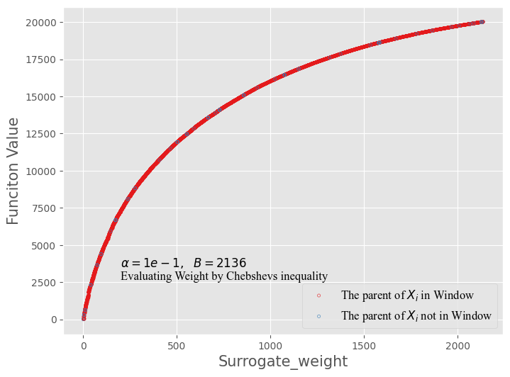
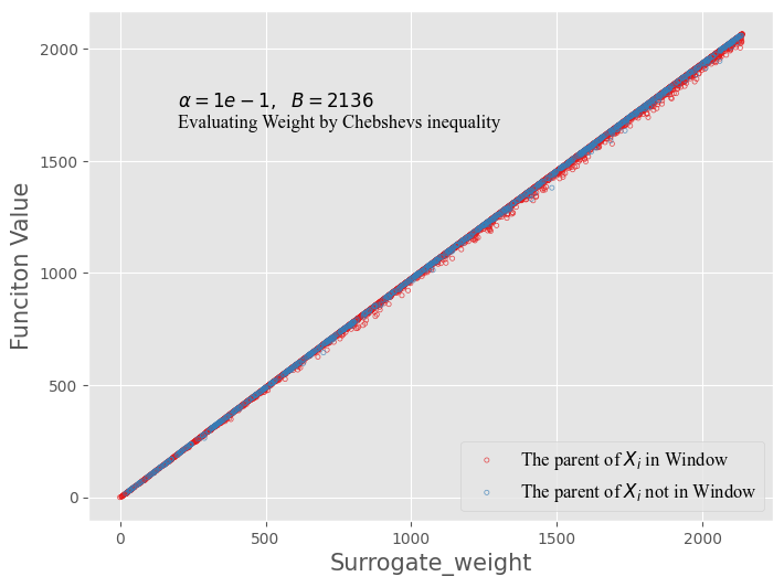
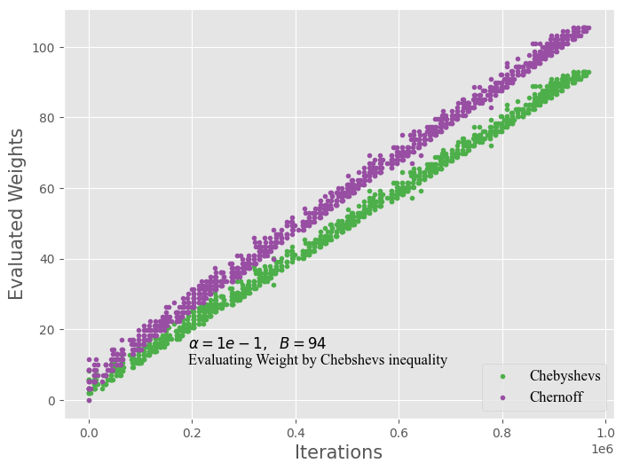
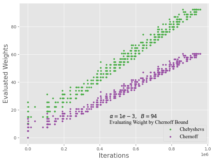
Table 3 shows the average number of trade-off solutions obtained by the GSEMO and SW-GSEMO using different surrogate functions on the problem based on the graph ca-CondaMat with IID weights. Notably, the SW-GSEMO produces a greater number of trade-off solutions in the final population than the GSEMO, particularly as the bound increases. Furthermore, the table reveals that the number of solutions in the population is consistently lower than (as defined in Section 4.1, where ). When comparing with the deterministic setting, it is observed that the number of trade-off solutions generated by the algorithms in the IID weight setting decreases by almost 50% when , particularly when using the surrogate function based on one-sided Chebyshev’s inequality.
5.2.2 Visualization of SW-GSEMO
To focus on the SW-GSEMO’s performance in optimizing chance-constrained problems, Figures 1(a) and 1(b) offer an illustrative example of the optimization process. The figures illustrate the relationship between the surrogate weight and the function value of the solutions selected for the population, with different colors labeling solutions based on whether their parents were within the defined weight window. Initially, an increase in function value corresponding to an increase in surrogate weight is observed. It’s noteworthy that the same surrogate weight might correspond to multiple distinct function values. According to the algorithm’s domination scheme, among solutions with the same surrogate weight, all except the one with the highest function value are eliminated from the population. Besides, the figures highlight that there are some periods where the SW-GSEMO is unable to include any individuals within the window (particularly when the expected weights are uniform). Despite these periods, the sliding window mechanism remains effective throughout the optimization process, aiding the algorithm in achieving satisfactory results. Additionally, those blue search points are also close to the Pareto front area and do not impact the final results.
Additionally, Figures 2(a) and 2(b) describe the changes in surrogate weights of solutions across iterations. A noticeable trend is that the sliding windows align the surrogate weights in a linear pattern, where the surrogate weight generally increases with more iterations. Figure 2(a) indicates that the surrogate weight derived from the one-sided Chebyshev’s inequality is lower than that from the Chernoff bound when . Conversely, Figure 2(b) shows the opposite trend when . Furthermore, due to the influence of the chance constraint, the sliding-selection method, when using the surrogate weight, allows only one individual within the window under the IID wights setting for the instances that are applied to the IID weights setting according to Figure 2(b), aligning with our analysis in Section 4.1.
6 Conclusion
In this paper, we investigated the use of SW-GSEMO on chance-constrained monotone submodular optimization problems with IID weights and uniform weights with the same dispersion. Surrogate functions based on Chebshev’s inequality and Chernoff bound have been applied to evaluate the chance constraint. We showed theoretically that the SW-GSEMO with the surrogate can reach the same approximation result in a more efficient way than the GSEMO that was studied in previous work. Furthermore, the algorithm is applied to the maximum coverage problem in the experiments and its results are compared with other multi-objective algorithms under variable instances constructed by different graphs. The experiments demonstrated that the window defined in SW-GSEMO is sliding in the weight interval during the optimization. Additionally, the obtained results show that the SW-GSEMO with the surrogate based on one-sided Chebyshev’s inequality performs better than the GSEMO and NSGA-II (with population sizes 20 and 100) among most of the instances when is larger, and the SW-GSEMO using the Chernoff bound works best when is smaller. For future work, it would be interesting to consider other generalized settings with different distributions and covariances as part of the chance-constrained formulation.
6.0.1 Acknowledgements
This work has been supported by the Australian Research Council (ARC) through grant FT200100536.
References
- [1] Charnes, A., Cooper, W.W.: Chance-constrained programming. Management science 6(1), 73–79 (1959)
- [2] Corder, G.W., Foreman, D.I.: Nonparametric statistics for non-statisticians (2011)
- [3] Corus, D., Lehre, P.K., Neumann, F.: The generalized minimum spanning tree problem: a parameterized complexity analysis of bi-level optimisation. In: Proceedings of the 15th annual conference on Genetic and evolutionary computation. pp. 519–526 (2013)
- [4] Doerr, B., Doerr, C., Neumann, A., Neumann, F., Sutton, A.: Optimization of chance-constrained submodular functions. In: Proceedings of the AAAI Conference on Artificial Intelligence. vol. 34, pp. 1460–1467 (2020)
- [5] Don, T.P., Neumann, A., Neumann, F.: The chance constrained travelling thief problem: Problem formulations and algorithms. In: Genetic and Evolutionary Computation Conference, GECCO 2024. ACM (2024), to appear
- [6] Feige, U.: A threshold of ln n for approximating set cover. Journal of the ACM (JACM) 45(4), 634–652 (1998)
- [7] Friedrich, T., He, J., Hebbinghaus, N., Neumann, F., Witt, C.: Analyses of simple hybrid algorithms for the vertex cover problem. Evolutionary Computation 17(1), 3–19 (2009)
- [8] Friedrich, T., Hebbinghaus, N., Neumann, F., He, J., Witt, C.: Approximating covering problems by randomized search heuristics using multi-objective models. In: Proceedings of the 9th annual conference on Genetic and evolutionary computation. pp. 797–804 (2007)
- [9] Iwamura, K., Liu, B.: A genetic algorithm for chance constrained programming. Journal of Information and Optimization sciences 17(2), 409–422 (1996)
- [10] Khuller, S., Moss, A., Naor, J.S.: The budgeted maximum coverage problem. Information processing letters 70(1), 39–45 (1999)
- [11] Kratsch, S., Lehre, P.K., Neumann, F., Oliveto, P.S.: Fixed parameter evolutionary algorithms and maximum leaf spanning trees: A matter of mutation. In: Parallel Problem Solving from Nature, PPSN XI: 11th International Conference, Kraków, Poland, September 11-15, 2010, Proceedings, Part I 11. pp. 204–213. Springer (2010)
- [12] Lehre, P.K., Qin, X.: More precise runtime analyses of non-elitist eas in uncertain environments. In: Proceedings of the Genetic and Evolutionary Computation Conference. pp. 1160–1168 (2021)
- [13] Leskovec, J., Krause, A., Guestrin, C., Faloutsos, C., VanBriesen, J., Glance, N.: Cost-effective outbreak detection in networks. In: Proceedings of the 13th ACM SIGKDD international conference on Knowledge discovery and data mining. pp. 420–429 (2007)
- [14] Lissovoi, A., Witt, C.: A runtime analysis of parallel evolutionary algorithms in dynamic optimization. Algorithmica 78, 641–659 (2017)
- [15] Miller, B.L., Wagner, H.M.: Chance constrained programming with joint constraints. Operations Research 13(6), 930–945 (1965)
- [16] Nemhauser, G.L., Wolsey, L.A., Fisher, M.L.: An analysis of approximations for maximizing submodular set functions—i. Mathematical programming 14(1), 265–294 (1978)
- [17] Neumann, A., Neumann, F.: Optimising monotone chance-constrained submodular functions using evolutionary multi-objective algorithms. In: Parallel Problem Solving from Nature - PPSN XVI - 16th International Conference, PPSN 2020, Proceedings, Part I. Lecture Notes in Computer Science, vol. 12269, pp. 404–417. Springer (2020)
- [18] Neumann, F., Pourhassan, M., Roostapour, V.: Analysis of evolutionary algorithms in dynamic and stochastic environments. Theory of evolutionary computation: recent developments in discrete optimization pp. 323–357 (2020)
- [19] Neumann, F., Sutton, A.M.: Runtime analysis of evolutionary algorithms for the knapsack problem with favorably correlated weights. In: International Conference on Parallel Problem Solving from Nature. pp. 141–152. Springer (2018)
- [20] Neumann, F., Witt, C.: On the runtime of randomized local search and simple evolutionary algorithms for dynamic makespan scheduling. In: 24th International Joint Conference on Artificial Intelligence. pp. 3742–3748. AAAI Press (2015)
- [21] Neumann, F., Witt, C.: Fast pareto optimization using sliding window selection. In: ECAI 2023, pp. 1771–1778. IOS Press (2023)
- [22] Pathiranage, I.H., Neumann, F., Antipov, D., Neumann, A.: Effective 2- and 3-objective moea/d approaches for the chance constrained knapsack problem. In: Genetic and Evolutionary Computation Conference, GECCO 2024. ACM (2024), to appear
- [23] Pathiranage, I.H., Neumann, F., Antipov, D., Neumann, A.: Using 3-objective evolutionary algorithms for the dynamic chance constrained knapsack problem. In: Genetic and Evolutionary Computation Conference, GECCO 2024. ACM (2024), to appear
- [24] Perera, K., Neumann, A.: Multi-objective evolutionary algorithms with sliding window selection for the dynamic chance-constrained knapsack problem. In: Genetic and Evolutionary Computation Conference, GECCO 2024. ACM (2024), to appear
- [25] Poojari, C.A., Varghese, B.: Genetic algorithm based technique for solving chance constrained problems. European journal of operational research 185(3), 1128–1154 (2008)
- [26] Roostapour, V., Neumann, A., Neumann, F.: On the performance of baseline evolutionary algorithms on the dynamic knapsack problem. In: International Conference on Parallel Problem Solving from Nature. pp. 158–169. Springer (2018)
- [27] Roostapour, V., Neumann, A., Neumann, F., Friedrich, T.: Pareto optimization for subset selection with dynamic cost constraints. Artificial Intelligence 302, 103597 (2022)
- [28] Rossi, R., Ahmed, N.: The network data repository with interactive graph analytics and visualization. In: Proceedings of the AAAI conference on artificial intelligence. vol. 29 (2015)
- [29] Shi, F., Neumann, F., Wang, J.: Runtime analysis of randomized search heuristics for the dynamic weighted vertex cover problem. In: Proceedings of the Genetic and Evolutionary Computation Conference. pp. 1515–1522 (2018)
- [30] Shi, F., Yan, X., Neumann, F.: Runtime analysis of simple evolutionary algorithms for the chance-constrained makespan scheduling problem. In: International Conference on Parallel Problem Solving from Nature. pp. 526–541. Springer (2022)
- [31] Wu, J., Polyakovskiy, S., Neumann, F.: On the impact of the renting rate for the unconstrained nonlinear knapsack problem. In: Proceedings of the Genetic and Evolutionary Computation Conference 2016. pp. 413–419 (2016)
- [32] Yan, X., Do, A.V., Shi, F., Qin, X., Neumann, F.: Optimizing chance-constrained submodular problems with variable uncertainties. In: ECAI 2023, pp. 2826–2833. IOS Press (2023)
- [33] Yan, X., Neumann, A., Neumann, F.: Sampling-based pareto optimization for chance-constrained monotone submodular problems. In: Genetic and Evolutionary Computation Conference, GECCO 2024. ACM (2024), to appear
- [34] Yaroslavtsev, G., Zhou, S., Avdiukhin, D.: “bring your own greedy”+ max: Near-optimal 1/2-approximations for submodular knapsack. In: International Conference on Artificial Intelligence and Statistics. pp. 3263–3274. PMLR (2020)
Appendix 0.A Tables
| GSEMO (1) | SW-GSEMO (2) | (3) | (4) | ||||||||||||
|---|---|---|---|---|---|---|---|---|---|---|---|---|---|---|---|
| Graph | Mean | std | stat | Mean | std | stat | Mean | std | stat | Mean | std | stat | |||
| ca-CSphd | 43 | 1500000 | 0.1 | 546 | 0 | 2(=),3(+),4(+) | 546 | 0 | 1(=),3(+),4(+) | 533.566 | 5.064 | 1(-),2(-),4(-) | 545.233 | 0.76 | 1(-),2(-),3(+) |
| 0.001 | 238 | 0 | 2(=),3(+),4(=) | 238 | 0 | 1(=),3(+),4(=) | 237.6 | 0.611 | 1(-),2(-),4(-) | 238 | 0 | 1(=),2(=),3(-) | |||
| 1000000 | 0.1 | 545.966 | 0.179 | 2(-),3(+),4(+) | 546 | 0 | 1(=),3(+),4(+) | 528.933 | 6.196 | 1(-),2(-),4(-) | 544.733 | 1.123 | 1(-),2(-),3(+) | ||
| 0.001 | 238 | 0 | 2(=),3(+),4(=) | 238 | 0 | 1(=),3(+),4(=) | 236.933 | 0.727 | 1(-),2(-),4(-) | 238 | 0 | 1(=),2(=),3(+) | |||
| 500000 | 0.1 | 543 | 2.065 | 2(-),3(+),4(-) | 546 | 0 | 1(+),3(+),4(+) | 517.266 | 8.35 | 1(-),2(-),4(-) | 543.533 | 1.477 | 1(+),2(-),3(+) | ||
| 0.001 | 238 | 0 | 2(=),3(+),4(+) | 238 | 0 | 1(=),3(+),4(+) | 235.966 | 1.538 | 1(-),2(-),4(-) | 237.9 | 0.3 | 1(-),2(-),3(+) | |||
| 94 | 1500000 | 0.1 | 880.993 | 0.727 | 2(-),3(+),4(+) | 883 | 0 | 1(-),3(+),4(+) | 857.766 | 6.173 | 1(-),2(-),4(-) | 870.133 | 2.753 | 1(-),2(-),3(+) | |
| 0.001 | 546 | 0 | 2(=),3(+),4(+) | 546 | 0 | 1(=),3(+),4(+) | 531.433 | 5.613 | 1(-),2(-),4(-) | 545.5 | 0.921 | 1(-),2(-),3(+) | |||
| 1000000 | 0.1 | 875.966 | 2.469 | 2(-),3(+),4(+) | 883 | 0 | 1(+),3(+),4(+) | 845.6 | 8.89 | 1(-),2(-),4(-) | 865.9 | 3.515 | 1(-),2(-),3(+) | ||
| 0.001 | 545.966 | 0.179 | 2(-),3(+),4(+) | 546 | 0 | 1(+),3(+),4(+) | 523.233 | 6.338 | 1(-),2(-),4(-) | 544.833 | 0.897 | 1(-),2(-),3(+) | |||
| 500000 | 0.1 | 848.533 | 4.1 | 2(-),3(+),4(-) | 882.766 | 0.422 | 1(+),3(+),4(+) | 821.733 | 10.168 | 1(-),2(-),4(-) | 858.4 | 3.878 | 1(+),2(-),3(+) | ||
| 0.001 | 543.1 | 1.738 | 2(-),3(+),4(-) | 546 | 0 | 1(+),3(+),4(+) | 511.333 | 8.117 | 1(-),2(-),4(-) | 543.366 | 1.471 | 1(+),2(-),3(+) | |||
| 188 | 1500000 | 0.1 | 1234.066 | 2.128 | 2(-),3(+),4(+) | 1243.233 | 0.76 | 1(+),3(+),4(+) | 1225 | 3.941 | 1(-),2(-),4(-) | 1220.433 | 3.602 | 1(-),2(-),3(+) | |
| 0.001 | 941.366 | 0.572 | 2(-),3(+),4(+) | 942.933 | 0.359 | 1(+),3(+),4(+) | 919.133 | 5.01 | 1(-),2(-),4(-) | 925.133 | 3.116 | 1(-),2(-),3(+) | |||
| 1000000 | 0.1 | 1213.96 | 3.281 | 2(-),3(+),4(-) | 1243.23 | 0.715 | 1(+),3(+),4(+) | 1210.866 | 6.781 | 1(-),2(-),4(-) | 1214.133 | 3.685 | 1(-),2(-),3(+) | ||
| 0.001 | 934.9 | 1.795 | 2(-),3(+),4(+) | 943 | 0 | 1(+),3(+),4(+) | 906 | 7.478 | 1(-),2(-),4(-) | 922.633 | 4.094 | 1(-),2(-),3(+) | |||
| 500000 | 0.1 | 1154.633 | 6.332 | 2(-),3(+),4(-) | 1243.466 | 0.618 | 1(+),3(+),4(+) | 1179.3 | 8.509 | 1(-),2(-),4(-) | 1200.766 | 5.308 | 1(+),2(-),3(+) | ||
| 0.001 | 903.7 | 5.386 | 2(-),3(+),4(-) | 942.933 | 0.249 | 1(+),3(+),4(+) | 876 | 12.492 | 1(-),2(-),4(-) | 915.5 | 4.883 | 1(+),2(-),3(+) | |||
| ca-GrQc | 64 | 1500000 | 0.1 | 1403.933 | 7.54 | 2(-),3(+),4(+) | 1432.333 | 1.534 | 1(+),3(+),4(+) | 1305.666 | 20.426 | 1(-),2(-),4(-) | 1395.9 | 11.527 | 1(-),2(-),3(+) |
| 0.001 | 754.266 | 3.14 | 2(+),3(+),4(-) | 756.933 | 0.249 | 1(-),3(+),4(-) | 724.7 | 9.212 | 1(-),2(-),4(-) | 754.7 | 2.368 | 1(+),2(+),3(+) | |||
| 1000000 | 0.1 | 1387.5 | 7.428 | 2(-),3(+),4(+) | 1431.733 | 2.644 | 1(+),3(+),4(+) | 1289.6 | 19.338 | 1(-),2(-),4(-) | 1386.26 | 12.465 | 1(-),2(-),3(+) | ||
| 0.001 | 746.033 | 7.323 | 2(-),3(+),4(-) | 756.966 | 0.179 | 1(+),3(+),4(-) | 717.066 | 13.132 | 1(-),2(-),4(-) | 753.033 | 2.96 | 1(+),2(+),3(+) | |||
| 500000 | 0.1 | 1332.466 | 12.831 | 2(-),3(+),4(-) | 1427.633 | 4.693 | 1(+),3(+),4(+) | 1233.9 | 19.618 | 1(-),2(-),4(-) | 1369.066 | 14.104 | 1(+),2(-),4(+) | ||
| 0.001 | 733.2 | 7.93 | 2(-),3(+),4(-) | 754.966 | 4.118 | 1(+),3(+),4(+) | 698.9 | 15.788 | 1(-),2(-),4(-) | 748.133 | 7.214 | 1(+),2(-),3(+) | |||
| 207 | 1500000 | 0.1 | 2516.2 | 13.929 | 2(-),3(+),4(-) | 2694.6 | 4.506 | 1(+),3(+),4(+) | 2428.466 | 21.846 | 1(-),2(-),4(-) | 2551.866 | 14.176 | 1(+),2(-),3(+) | |
| 0.001 | 1974.466 | 10.206 | 2(-),3(+),4(+) | 2053.9 | 3.279 | 1(+),3(+),4(+) | 1837.066 | 23.589 | 1(-),2(-),4(-) | 1968.566 | 16.111 | 1(-),2(-),3(+) | |||
| 1000000 | 0.1 | 2434.9 | 13.55 | 2(-),3(+),4(+) | 2691.466 | 4.462 | 1(+),3(+),4(+) | 2363.966 | 25.356 | 1(-),2(-),4(-) | 2535.766 | 16.823 | 1(+),2(-),3(+) | ||
| 0.001 | 1930.133 | 10.901 | 2(-),3(+),4(-) | 2054.833 | 3.652 | 1(+),3(+),4(+) | 1793.833 | 27.668 | 1(-),2(-),4(-) | 1958.7 | 18.018 | 1(-),2(-),3(+) | |||
| 500000 | 0.1 | 2288.033 | 14.549 | 2(-),3(+),4(-) | 2688 | 6.957 | 1(+),3(+),4(+) | 2230.6 | 26.925 | 1(-),2(-),4(-) | 2487.6 | 23.171 | 1(-),2(-),3(+) | ||
| 0.001 | 1821.933 | 13.985 | 2(-),3(+),4(-) | 2049.1 | 5.081 | 1(+),3(+),4(+) | 1704.366 | 30.625 | 1(-),2(-),4(-) | 1925.133 | 16.202 | 1(-),2(-),3(+) | |||
| 415 | 1500000 | 0.1 | 3205.966 | 12.605 | 2(-),3(-),4(-) | 3556.866 | 3.518 | 1(+),3(+),4(+) | 3270.966 | 23.345 | 1(+),2(-),4(-) | 3296.6 | 14.63 | 1(-),2(-),3(+) | |
| 0.001 | 2822.733 | 13.053 | 2(-),3(+),4(-) | 3078.9 | 4.407 | 1(+),3(+),4(+) | 2777.2 | 17.158 | 1(-),2(-),4(-) | 2865.933 | 16.29 | 1(-),2(-),3(+) | |||
| 1000000 | 0.1 | 3105 | 11.195 | 2(-),3(-),4(-) | 3555.3 | 4.267 | 1(+),3(+),4(+) | 3179.033 | 22.15 | 1(+),2(-),4(-) | 3264.433 | 14.718 | 1(-),2(-),3(+) | ||
| 0.001 | 2734.76 | 13.934 | 2(-),3(+),4(-) | 3076.2 | 4.867 | 1(+),3(+),4(+) | 2688.73 | 28.249 | 1(-),2(-),4(-) | 2832.9 | 16.933 | 1(-),2(-),3(+) | |||
| 500000 | 0.1 | 2921.366 | 18.076 | 2(-),3(-),4(-) | 3548.8 | 4.969 | 1(+),3(+),4(+) | 3000.266 | 25.241 | 1(+),2(-),4(-) | 3198.266 | 17.804 | 1(-),2(-),3(+) | ||
| 0.001 | 2569.566 | 17.657 | 2(-),3(+),4(-) | 3070.5 | 6.206 | 1(+),3(+),4(+) | 2525.533 | 30.721 | 1(-),2(-),4(-) | 2774.433 | 17.44 | 1(-),2(-),3(+) | |||
| ca-CondaMat | 146 | 1500000 | 0.1 | 5588 | 47.265 | 2(-),3(+),4(-) | 6790.966 | 12.335 | 1(+),3(+),4(+) | 5187.966 | 95.708 | 1(-),2(-),4(-) | 6330.3 | 36.893 | 1(+),2(-),3(+) |
| 0.001 | 4153.733 | 43.338 | 2(-),3(+),4(-) | 4748.166 | 7.585 | 1(+),3(+),4(+) | 3802.733 | 75.95 | 1(-),2(-),4(-) | 4531.83 | 33.061 | 1(+),2(-),3(+) | |||
| 1000000 | 0.1 | 5500.73 | 47.67 | 2(-),3(+),4(-) | 6771.366 | 16.3 | 1(+),3(+),4(+) | 4945.9 | 113.293 | 1(-),2(-),4(-) | 6281 | 46.322 | 1(+),2(-),3(+) | ||
| 0.001 | 3957.5 | 40.782 | 2(-),3(+),4(-) | 4736.133 | 10.375 | 1(+),3(+),4(+) | 3709.06 | 96.656 | 1(-),2(-),4(-) | 4496.7 | 28.765 | 1(+),2(-),3(+) | |||
| 500000 | 0.1 | 4818.53 | 47.71 | 2(-),3(+),4(-) | 6708.366 | 27.316 | 1(+),3(+),4(+) | 4685.333 | 114.8373 | 1(-),2(-),4(-) | 6115.233 | 54.393 | 1(+),2(-),3(+) | ||
| 0.001 | 3648.3 | 65.33 | 2(-),3(+),4(-) | 4581.633 | 36.88 | 1(+),3(+),4(+) | 3469.766 | 73.953 | 1(-),2(-),4(-) | 4395.566 | 43.076 | 1(+),2(-),3(+) | |||
| 1068 | 1500000 | 0.1 | 11787.533 | 57.133 | 2(-),3(+),4(-) | 16650.933 | 14.163 | 1(+),3(+),4(+) | 12284.866 | 142.248 | 1(-),2(-),4(-) | 13394.133 | 75.448 | 1(+),2(-),3(+) | |
| 0.001 | 10893.9 | 61.683 | 2(-),3(+),4(-) | 15217.3 | 14.45 | 1(+),3(+),4(+) | 10950.3 | 122.3 | 1(-),2(-),4(-) | 12241.966 | 72.716 | 1(+),2(-),3(+) | |||
| 1000000 | 0.1 | 11194.23 | 72.488 | 2(-),3(-),4(-) | 16573.6 | 19.608 | 1(+),3(+),4(+) | 11623.93 | 119.467 | 1(+),2(-),4(-) | 13164.2 | 60.07 | 1(+),2(-),3(+) | ||
| 0.001 | 10364.53 | 58.95 | 2(-),3(+),4(-) | 15145.666 | 14.485 | 1(+),3(+),4(+) | 9987.13 | 123.936 | 1(-),2(-),4(-) | 12040.166 | 99.78 | 1(+),2(-),3(+) | |||
| 500000 | 0.1 | 9474.733 | 111.851 | 2(-),3(-),4(-) | 16368.6 | 27.005 | 1(+),3(+),4(+) | 10729.133 | 180.573 | 1(+),2(-),4(-) | 12708.533 | 82.447 | 1(+),2(-),3(+) | ||
| 0.001 | 9344.733 | 84.931 | 2(-),3(-),4(-) | 14947.6 | 22.553 | 1(+),3(+),4(+) | 9502.2 | 142.003 | 1(+),2(-),4(-) | 11581.066 | 84.55 | 1(+),2(-),3(+) | |||
| 2136 | 1500000 | 0.1 | 12749.533 | 93.378 | 2(-),3(-),4(-) | 20078.833 | 11.066 | 1(+),3(+),4(+) | 16361.766 | 67.76 | 1(+),2(-),4(-) | 16243.166 | 68.601 | 1(+),2(-),3(+) | |
| 0.001 | 12730.3 | 91.025 | 2(-),3(-),4(-) | 19327.433 | 11.221 | 1(+),3(+),4(+) | 15224.733 | 66.313 | 1(+),2(-),4(-) | 15402.133 | 96.35 | 1(+),2(-),3(+) | |||
| 1000000 | 0.1 | 11520.966 | 129.843 | 2(-),3(-),4(-) | 20016.2 | 16.172 | 1(+),3(+),4(+) | 15696.5 | 116.216 | 1(+),2(-),4(-) | 16020.633 | 88.739 | 1(+),2(-),3(+) | ||
| 0.001 | 11500.633 | 114.875 | 2(-),3(-),4(-) | 19245.233 | 15.532 | 1(+),3(+),4(+) | 14544.63 | 98.014 | 1(+),2(-),4(-) | 15155.4 | 74.248 | 1(+),2(-),3(+) | |||
| 500000 | 0.1 | 9488.333 | 90.631 | 2(-),3(-),4(-) | 19822.566 | 20.619 | 1(+),3(+),4(+) | 14592.466 | 104.587 | 1(+),2(-),4(-) | 14734.2 | 230.948 | 1(+),2(-),3(+) | ||
| 0.001 | 9483.6 | 88.03 | 2(-),3(-),4(-) | 19030.533 | 21.451 | 1(+),3(+),4(+) | 13456.133 | 89.165 | 1(+),2(-),4(-) | 14399.233 | 152.192 | 1(+),2(-),3(+) | |||
| GSEMO (5) | SW-GSEMO (6) | (7) | (8) | ||||||||||||
|---|---|---|---|---|---|---|---|---|---|---|---|---|---|---|---|
| Graph | Mean | std | stat | Mean | std | stat | Mean | std | stat | Mean | std | stat | |||
| ca-CSphd | 43 | 1500000 | 0.1 | 478 | 0 | 6(=),7(+),8(+) | 478 | 0 | 5(=),7(+),8(+) | 468.333 | 4.853 | 5(-),6(-),8(-) | 477.766 | 0.495 | 5(-),6(-),7(+) |
| 0.001 | 413 | 0 | 6(=),7(+),8(+) | 413 | 0 | 5(=),7(+),8(+) | 405.4 | 3.903 | 5(-),6(-),8(-) | 412.9 | 0.3 | 5(-),6(-),7(+) | |||
| 1000000 | 0.1 | 478 | 0 | 6(=),7(+),8(+) | 478 | 0 | 5(=),7(+),8(+) | 463 | 5.403 | 5(-),6(-),8(-) | 477.7 | 0.781 | 5(-),6(-),7(+) | ||
| 0.001 | 413 | 0 | 6(=),7(+),8(+) | 413 | 0 | 5(=),7(+),8(+) | 402.6 | 4.24 | 5(-),6(-),8(-) | 412.633 | 0.481 | 5(-),6(-),7(+) | |||
| 500000 | 0.1 | 477.966 | 0.179 | 6(-),7(+),8(+) | 477.966 | 0.179 | 5(+),7(+),8(+) | 453.566 | 7.269 | 5(-),6(-),8(-) | 477.166 | 0.968 | 5(-),6(-),7(+) | ||
| 0.001 | 412.9 | 0.3 | 6(-),7(+),8(+) | 413 | 0 | 5(+),7(+),8(+) | 396 | 5.196 | 5(-),6(-),8(-) | 412.066 | 0.771 | 5(-),6(-),7(+) | |||
| 94 | 1500000 | 0.1 | 817.7 | 0.525 | 6(-),7(+),8(+) | 818 | 0 | 5(+),7(+),8(+) | 796.7 | 5.484 | 5(-),6(-),8(-) | 808.933 | 3.14 | 5(-),6(-),7(+) | |
| 0.001 | 749.633 | 0 | 6(-),7(+),8(+) | 750 | 0 | 5(+),7(+),8(+) | 729.066 | 5.938 | 5(-),6(-),8(-) | 743 | 2.081 | 5(-),6(-),7(+) | |||
| 1000000 | 0.1 | 817.5 | 0.67 | 6(-),7(+),8(+) | 817.966 | 0.179 | 5(+),7(+),8(+) | 785.766 | 7.218 | 5(-),6(-),8(-) | 806.9 | 3.703 | 5(-),6(-),7(+) | ||
| 0.001 | 749.633 | 0.546 | 6(-),7(+),8(+) | 750 | 0 | 5(+),7(+),8(+) | 718.466 | 7.658 | 5(-),6(-),8(-) | 740.5 | 2.86 | 5(-),6(-),7(+) | |||
| 500000 | 0.1 | 809.8 | 1.956 | 6(-),7(+),8(+) | 818 | 0 | 5(+),7(+),8(+) | 764.733 | 9.337 | 5(-),6(-),8(-) | 800.766 | 3.48 | 5(-),6(-),7(+) | ||
| 0.001 | 744.633 | 2.057 | 6(-),7(+),8(+) | 749.96 | 0.179 | 5(+),7(+),8(+) | 695 | 9.855 | 5(-),6(-),8(-) | 735.666 | 4.307 | 5(-),6(-),7(+) | |||
| 188 | 1500000 | 0.1 | 1181.733 | 2.542 | 6(-),7(+),8(+) | 1192.466 | 0.618 | 5(+),7(+),8(+) | 1166.966 | 5.003 | 5(-),6(-),8(-) | 1166.966 | 3.772 | 5(-),6(-),7(+) | |
| 0.001 | 1120.6 | 1.89 | 6(-),7(+),8(+) | 1128 | 0 | 5(+),7(+),8(+) | 1103.5 | 4.595 | 5(-),6(-),8(-) | 1105.8 | 3.572 | 5(-),6(-),7(+) | |||
| 1000000 | 0.1 | 1181.233 | 2.216 | 6(-),7(+),8(+) | 1192.3 | 0.69 | 5(+),7(+),8(+) | 1153.766 | 5.696 | 5(-),6(-),8(-) | 1160.033 | 3.745 | 5(-),6(-),7(+) | ||
| 0.001 | 1120.633 | 1.957 | 6(-),7(+),8(+) | 1127.966 | 0.179 | 5(+),7(+),8(+) | 1090.766 | 6.907 | 5(-),6(-),8(-) | 1099.6 | 2.961 | 5(-),6(-),7(+) | |||
| 500000 | 0.1 | 1143.833 | 5.865 | 6(-),7(+),8(-) | 1192.366 | 0.546 | 5(+),7(+),8(+) | 1122.1 | 8.904 | 5(-),6(-),8(-) | 1147.166 | 4.993 | 5(+),6(-),7(+) | ||
| 0.001 | 1089.333 | 4.101 | 6(-),7(+),8(+) | 1127.9 | 0.3 | 5(+),7(+),8(+) | 1057.266 | 10.327 | 5(-),6(-),8(-) | 1089.166 | 4.719 | 5(-),6(-),7(+) | |||
| ca-GrQc | 64 | 1500000 | 0.1 | 1275.6 | 6.311 | 6(-),7(+),8(+) | 1294.433 | 2.076 | 5(+),7(+),8(+) | 1189.966 | 17.809 | 5(-),6(-),8(-) | 1265.633 | 6.695 | 5(-),6(-),7(+) |
| 0.001 | 1125.76 | 5.69 | 6(-),7(+),8(+) | 1145.433 | 0.955 | 5(+),7(+),8(+) | 1054.733 | 18.446 | 5(-),6(-),8(-) | 1125.2 | 7.409 | 5(-),6(-),7(+) | |||
| 1000000 | 0.1 | 1275.233 | 7.548 | 6(-),7(+),8(+) | 1294.1 | 2.399 | 5(+),7(+),8(+) | 1168.6 | 16.318 | 5(-),6(-),8(-) | 1259.266 | 10.478 | 5(-),6(-),7(+) | ||
| 0.001 | 1127.3 | 7.528 | 6(-),7(+),8(+) | 1144.866 | 1.431 | 5(+),7(+),8(+) | 1031.1 | 19.291 | 5(-),6(-),8(-) | 1121.933 | 8.156 | 5(-),6(-),7(+) | |||
| 500000 | 0.1 | 1249.5 | 11.242 | 6(-),7(+),8(+) | 1291.6 | 4.095 | 5(+),7(+),8(+) | 1126.333 | 21.235 | 5(-),6(-),8(-) | 1246 | 13.147 | 5(-),6(-),7(+) | ||
| 0.001 | 1105.533 | 8.815 | 6(-),7(+),8(+) | 1143.266 | 2.112 | 5(+),7(+),8(+) | 992.333 | 19.777 | 5(-),6(-),8(-) | 1112.933 | 9.44 | 5(-),6(-),7(+) | |||
| 207 | 1500000 | 0.1 | 2426.533 | 10.704 | 6(-),7(+),8(-) | 2585.5 | 4.514 | 5(+),7(+),8(+) | 2321.133 | 29.9 | 5(-),6(-),8(-) | 2454.966 | 16.664 | 5(+),6(-),7(+) | |
| 0.001 | 2316.666 | 9.133 | 6(-),7(+),8(-) | 2452.633 | 4.956 | 5(+),7(+),8(+) | 2205.166 | 19.834 | 5(-),6(-),8(-) | 2328.2 | 19.436 | 5(+),6(-),7(+) | |||
| 1000000 | 0.1 | 2425.333 | 13.196 | 6(-),7(+),8(-) | 2582 | 5.899 | 5(+),7(+),8(+) | 2258.666 | 25.941 | 5(-),6(-),8(-) | 2437.7 | 13.256 | 5(+),6(-),7(+) | ||
| 0.001 | 2315.7666 | 10.4 | 6(-),7(+),8(+) | 2450.066 | 5.585 | 5(+),7(+),8(+) | 2151.4 | 34.358 | 5(-),6(-),8(-) | 2313.766 | 17.392 | 5(-),6(-),7(+) | |||
| 500000 | 0.1 | 2294.366 | 13.212 | 6(-),7(+),8(-) | 2577.566 | 6.751 | 5(+),7(+),8(+) | 2133.1 | 32.639 | 5(-),6(-),8(-) | 2396.5 | 12.241 | 5(+),6(-),7(+) | ||
| 0.001 | 2194.233 | 13.142 | 6(-),7(+),8(+) | 2446.233 | 5.69 | 5(+),7(+),8(+) | 2028.766 | 34.202 | 5(-),6(-),8(-) | 2276.9 | 16.44 | 5(-),6(-),7(+) | |||
| 415 | 1500000 | 0.1 | 3142.9 | 10.746 | 6(-),7(-),8(-) | 3479.133 | 3.77 | 5(+),7(+),8(+) | 3182.9 | 20.115 | 5(+),6(-),8(-) | 3227.633 | 16.15 | 5(+),6(-),7(+) | |
| 0.001 | 3069.366 | 15.047 | 6(-),7(-),8(-) | 3394.733 | 4.17 | 5(+),7(+),8(+) | 3080.033 | 17.564 | 5(+),6(-),8(-) | 3140.2 | 17.457 | 5(+),6(-),7(+) | |||
| 1000000 | 0.1 | 3133.366 | 12.768 | 6(-),7(+),8(-) | 3477.833 | 4.568 | 5(+),7(+),8(+) | 3098.233 | 27.465 | 5(-),6(-),8(-) | 3194.066 | 18.145 | 5(+),6(-),7(+) | ||
| 0.001 | 3055.366 | 13.496 | 6(-),7(+),8(-) | 3391.766 | 4.63 | 5(+),7(+),8(+) | 2999.766 | 35.903 | 5(-),6(-),8(-) | 3105.633 | 17.516 | 5(+),6(-),7(+) | |||
| 500000 | 0.1 | 2949.733 | 14.955 | 6(-),7(+),8(-) | 3470.666 | 4.763 | 5(+),7(+),8(+) | 2920.233 | 35.273 | 5(-),6(-),8(-) | 3127.566 | 16.562 | 5(+),6(-),7(+) | ||
| 0.001 | 2874.9 | 14.767 | 6(-),7(+),8(-) | 3382.833 | 4.442 | 5(+),7(+),8(+) | 2836 | 32.535 | 5(-),6(-),8(-) | 3039.433 | 17.562 | 5(+),6(-),7(+) | |||
| ca-CondaMat | 146 | 1500000 | 0.1 | 5321.1333 | 40.291 | 6(-),7(+),8(-) | 6424.2 | 10.403 | 5(+),7(+),8(+) | 4931.833 | 82.145 | 5(-),6(-),8(-) | 6018.066 | 41.946 | 5(+),6(-),7(+) |
| 0.001 | 5027.166 | 49.31 | 6(-),7(+),8(-) | 5994.833 | 10.96 | 5(+),7(+),8(+) | 4622.866 | 96.07 | 5(-),6(-),8(-) | 5652.833 | 41.121 | 5(+),6(-),7(+) | |||
| 1000000 | 0.1 | 5059.6 | 39.678 | 6(-),7(+),8(-) | 6397.966 | 14.943 | 5(+),7(+),8(+) | 4755.133 | 73.411 | 5(-),6(-),8(-) | 5954.966 | 50.251 | 5(+),6(-),7(+) | ||
| 0.001 | 4784.766 | 54.93 | 6(-),7(+),8(-) | 5979.9 | 16.912 | 5(+),7(+),8(+) | 4441.5 | 126.327 | 5(-),6(-),8(-) | 5582.666 | 38.694 | 5(+),6(-),7(+) | |||
| 500000 | 0.1 | 4625.4 | 60.563 | 6(-),7(+),8(-) | 6328.2 | 31.971 | 5(+),7(+),8(+) | 4443.2 | 84.517 | 5(-),6(-),8(-) | 5787.266 | 63.911 | 5(+),6(-),7(+) | ||
| 0.001 | 4344.33 | 59.972 | 6(-),7(+),8(-) | 5898.133 | 22.47 | 5(+),7(+),8(+) | 4170 | 103.826 | 5(-),6(-),8(-) | 5437.7 | 43.076 | 5(+),6(-),7(+) | |||
| 1068 | 1500000 | 0.1 | 11632.833 | 52.573 | 6(-),7(-),8(-) | 16650.933 | 14.163 | 5(+),7(+),8(+) | 12054.233 | 126.656 | 5(+),6(-),8(-) | 13206.26 | 65.605 | 5(+),6(-),7(+) | |
| 0.001 | 11464.966 | 61.738 | 6(-),7(-),8(-) | 15217.3 | 14.45 | 5(+),7(+),8(+) | 11783.9 | 95.969 | 5(+),6(-),8(-) | 12974.86 | 85.587 | 5(+),6(-),7(+) | |||
| 1000000 | 0.1 | 11059.2 | 73.482 | 6(-),7(-),8(-) | 16343.833 | 16.806 | 5(+),7(+),8(+) | 11441.2 | 145.704 | 5(+),6(-),8(-) | 12961.266 | 85.324 | 5(+),6(-),7(+) | ||
| 0.001 | 10914.833 | 76.11 | 6(-),7(-),8(-) | 16052.866 | 19.687 | 5(+),7(+),8(+) | 11208.1 | 91.525 | 5(+),6(-),8(-) | 12779.033 | 59.812 | 5(+),6(-),7(+) | |||
| 500000 | 0.1 | 9482.966 | 92.698 | 6(-),7(-),8(-) | 16129.133 | 27.284 | 5(+),7(+),8(+) | 10487.566 | 128.411 | 5(+),6(-),8(-) | 12489.3 | 88.034 | 5(+),6(-),7(+) | ||
| 0.001 | 9466.433 | 113.403 | 6(-),7(-),8(-) | 15840.433 | 26.94 | 5(+),7(+),8(+) | 10254.133 | 130.19 | 5(+),6(-),8(-) | 12309.4 | 81.884 | 5(+),6(-),7(+) | |||
| 2136 | 1500000 | 0.1 | 12719.533 | 106.011 | 6(-),7(-),8(-) | 19955.3 | 10.312 | 5(+),7(+),8(+) | 16187.466 | 93.583 | 5(+),6(-),8(-) | 16130.1 | 80.711 | 5(+),6(-),7(+) | |
| 0.001 | 12701.7 | 90.339 | 6(-),7(-),8(-) | 19813.8 | 14.041 | 5(+),7(+),8(+) | 16006.8 | 109.226 | 5(+),6(-),8(-) | 15964.933 | 75.003 | 5(+),6(-),7(+) | |||
| 1000000 | 0.1 | 11481.066 | 98.619 | 6(-),7(-),8(-) | 19891.466 | 13.197 | 5(+),7(+),8(+) | 15519.3 | 102.403 | 5(+),6(-),8(-) | 15812.433 | 93.623 | 5(+),6(-),7(+) | ||
| 0.001 | 11458.1 | 116.396 | 6(-),7(-),8(-) | 19750.366 | 12.084 | 5(+),7(+),8(+) | 15323.266 | 103.988 | 5(+),6(-),8(-) | 15684.533 | 83.137 | 5(+),6(-),7(+) | |||
| 500000 | 0.1 | 9451.033 | 105.529 | 6(-),7(-),8(-) | 19697.033 | 17.995 | 5(+),7(+),8(+) | 14435.233 | 101.01 | 5(+),6(-),8(-) | 14650.033 | 289.611 | 5(+),6(-),7(+) | ||
| 0.001 | 9460.666 | 116.783 | 6(-),7(-),8(-) | 19540.266 | 18.77 | 5(+),7(+),8(+) | 14218.8 | 129.106 | 5(+),6(-),8(-) | 14586.566 | 214.181 | 5(+),6(-),7(+) | |||
| GSEMO (9) | SW-GSEMO (10) | (11) | (12) | ||||||||||||
| Graph | Mean | std | stat | Mean | std | stat | Mean | std | stat | Mean | std | stat | |||
| ca-CSphd | 43 | 1500000 | 0.1 | 38 | 0 | 10(=),11(=),12(=) | 38 | 0 | 9(=),11(=),12(=) | 38 | 0 | 9(=),10(=),12(=) | 38 | 0 | 9(=),10(=),11(=) |
| 0.001 | 22 | 0 | 10(=),11(=),12(=) | 22 | 0 | 9(=),11(=),12(=) | 22 | 0 | 9(=),10(=),12(=) | 22 | 0 | 9(=),10(=),11(=) | |||
| 1000000 | 0.1 | 38 | 0 | 10(=),11(=),12(=) | 38 | 0 | 9(=),11(=),12(=) | 38 | 0 | 9(=),10(=),12(=) | 38 | 0 | 9(=),10(=),11(=) | ||
| 0.001 | 22 | 0 | 10(=),11(=),12(=) | 22 | 0 | 9(=),11(=),12(=) | 22 | 0 | 9(=),10(=),12(=) | 22 | 0 | 9(=),10(=),11(=) | |||
| 500000 | 0.1 | 38 | 0 | 10(=),11(=),12(=) | 38 | 0 | 9(=),11(=),12(=) | 38 | 0 | 9(=),10(=),12(=) | 38 | 0 | 9(=),10(=),11(=) | ||
| 0.001 | 22 | 0 | 10(=),11(=),12(=) | 22 | 0 | 9(=),11(=),12(=) | 22 | 0 | 9(=),10(=),12(=) | 22 | 0 | 9(=),10(=),11(=) | |||
| 94 | 1500000 | 0.1 | 88 | 0 | 10(=),11(=),12(=) | 88 | 0 | 9(=),11(=),12(=) | 87.733 | 0.442 | 9(=),10(=),12(=) | 88 | 0 | 9(=),10(=),11(=) | |
| 0.001 | 65 | 0 | 10(=),11(=),12(=) | 65 | 0 | 9(=),11(=),12(=) | 65 | 0 | 9(=),10(=),12(=) | 65 | 0 | 9(=),10(=),11(=) | |||
| 1000000 | 0.1 | 88 | 0 | 10(=),11(=),12(=) | 88 | 0 | 9(=),11(=),12(=) | 87.7 | 0.458 | 9(=),10(=),12(=) | 88 | 0 | 9(=),10(=),11(=) | ||
| 0.001 | 65 | 0 | 10(=),11(=),12(=) | 65 | 0 | 9(=),11(=),12(=) | 65 | 0 | 9(=),10(=),12(=) | 65 | 0 | 9(=),10(=),11(=) | |||
| 500000 | 0.1 | 88 | 0 | 10(-),11(=),12(=) | 88 | 0 | 9(+),11(+),12(+) | 87.633 | 5.467 | 9(=),10(-),12(=) | 87.966 | 0.179 | 9(=),10(-),11(=) | ||
| 0.001 | 65 | 0 | 10(=),11(=),12(=) | 65 | 0 | 9(=),11(=),12(=) | 65 | 0 | 9(=),10(=),12(=) | 65 | 0 | 9(=),10(=),11(=) | |||
| 188 | 1500000 | 0.1 | 175 | 0 | 10(=),11(+),12(=) | 175 | 0 | 9(=),11(+),12(=) | 172.733 | 0.928 | 9(-),10(-),12(-) | 175 | 0 | 9(=),10(=),11(+) | |
| 0.001 | 137 | 0 | 10(=),11(=),12(=) | 137 | 0 | 9(=),11(=),12(=) | 137 | 0 | 9(=),10(=),12(=) | 137 | 0 | 9(=),10(=),11(=) | |||
| 1000000 | 0.1 | 175 | 0 | 10(=),11(+),12(=) | 175 | 0 | 9(=),11(=),12(=) | 172.4 | 0.84 | 9(-),10(-),12(-) | 175 | 0 | 9(=),10(=),11(+) | ||
| 0.001 | 137 | 0 | 10(=),11(=),12(=) | 137 | 0 | 9(=),11(=),12(=) | 137 | 0 | 9(=),10(=),12(=) | 137 | 0 | 9(=),10(=),11(=) | |||
| 500000 | 0.1 | 174.966 | 0.179 | 10(=),11(+),12(=) | 175 | 0 | 9(=),11(=),12(=) | 171.466 | 0.884 | 9(-),10(-),12(-) | 175 | 0 | 9(=),10(=),11(+) | ||
| 0.001 | 137 | 0 | 10(=),11(=),12(=) | 137 | 0 | 9(=),11(=),12(=) | 137 | 0 | 9(=),10(=),12(=) | 137 | 0 | 9(=),10(=),11(=) | |||
| ca-GrQc | 64 | 1500000 | 0.1 | 60.966 | 0.179 | 10(=),11(=),12(=) | 61 | 0 | 9(=),11(=),12(=) | 60.933 | 0.249 | 9(=),10(=),12(=) | 61 | 0 | 9(=),10(=),11(=) |
| 0.001 | 44 | 0 | 10(=),11(=),12(=) | 44 | 0 | 9(=),11(=),12(=) | 44 | 0 | 9(=),10(=),12(=) | 44 | 0 | 9(=),10(=),11(=) | |||
| 1000000 | 0.1 | 60.9 | 0.3 | 10(=),11(=),12(=) | 61 | 0 | 9(=),11(=),12(=) | 60.766 | 0.422 | 9(=),10(=),12(=) | 61 | 0 | 9(=),10(=),11(=) | ||
| 0.001 | 44 | 0 | 10(=),11(=),12(=) | 44 | 0 | 9(=),11(=),12(=) | 44 | 0 | 9(=),10(=),12(=) | 44 | 0 | 9(=),10(=),11(=) | |||
| 500000 | 0.1 | 60.566 | 0.667 | 10(=),11(=),12(=) | 60.933 | 0.249 | 9(=),11(=),12(=) | 60.433 | 0.76 | 9(=),10(=),12(=) | 61 | 0 | 9(=),10(=),11(=) | ||
| 0.001 | 43.9 | 0.3 | 10(=),11(=),12(=) | 44 | 0 | 9(=),11(=),12(=) | 44 | 0 | 9(=),10(=),12(=) | 44 | 0 | 9(=),10(=),11(=) | |||
| 207 | 1500000 | 0.1 | 199 | 0 | 10(=),11(=),12(=) | 199 | 0 | 9(=),11(=),12(=) | 198 | 0.7745 | 9(=),10(=),12(=) | 199 | 0 | 9(=),10(=),11(=) | |
| 0.001 | 171.833 | 0.372 | 10(=),11(=),12(=) | 172 | 0 | 9(=),11(=),12(=) | 171.766 | 0.495 | 9(=),10(=),12(=) | 172 | 0 | 9(=),10(=),11(=) | |||
| 1000000 | 0.1 | 199 | 0 | 10(=),11(-),12(=) | 199 | 0 | 9(=),11(+),12(=) | 197.766 | 0.882 | 9(-),10(-),12(-) | 199 | 0 | 9(=),10(=),11(+) | ||
| 0.001 | 171.5 | 0.806 | 10(=),11(=),12(=) | 172 | 0 | 9(=),11(=),12(=) | 171.466 | 1.175 | 9(=),10(=),12(=) | 172 | 0 | 9(=),10(=),11(=) | |||
| 500000 | 0.1 | 198.766 | 0.422 | 10(=),11(=),12(=) | 199 | 0 | 9(=),11(=),12(=) | 197.266 | 1.236 | 9(=),10(=),12(=) | 198.96 | 0.179 | 9(=),10(=),11(=) | ||
| 0.001 | 169.466 | 1.707 | 10(=),11(-),12(-) | 171.966 | 0.179 | 9(=),11(-),12(-) | 171.066 | 1.364 | 9(=),10(=),12(=) | 172 | 0 | 9(+),10(+),11(=) | |||
| 415 | 1500000 | 0.1 | 398.266 | 0.442 | 10(=),11(+),12(=) | 399 | 0 | 9(=),11(+),12(=) | 390.966 | 1.622 | 9(-),10(-),12(-) | 398.466 | 0.498 | 9(=),10(=),11(+) | |
| 0.001 | 353.066 | 1.436 | 10(=),11(+),12(=) | 355 | 0 | 9(=),11(+),12(=) | 346.366 | 2.676 | 9(-),10(-),12(-) | 354.533 | 0.498 | 9(=),10(=),11(+) | |||
| 1000000 | 0.1 | 397.933 | 0.442 | 10(=),11(+),12(=) | 399 | 0 | 9(=),11(+),12(=) | 390.066 | 1.931 | 9(-),10(-),12(-) | 398.366 | 0.546 | 9(=),10(=),11(+) | ||
| 0.001 | 351.7 | 1.159 | 10(-),11(+),12(-) | 354.9 | 0.3 | 9(+),11(+),12(=) | 345.733 | 2.379 | 9(-),10(-),12(-) | 354.5 | 0.562 | 9(+),10(=),11(+) | |||
| 500000 | 0.1 | 396.933 | 0.512 | 10(-),11(+),12(=) | 398.766 | 0.422 | 9(+),11(+),12(=) | 388.333 | 2.102 | 9(-),10(-),12(-) | 397.866 | 0.6699 | 9(+),10(=),11(+) | ||
| 0.001 | 350 | 1.181 | 10(-),11(+),12(-) | 354.533 | 0.669 | 9(+),11(+),12(-) | 344.066 | 2.644 | 9(-),10(-),12(-) | 354.333 | 0.596 | 9(+),10(+),11(+) | |||
| ca-CondaMat | 146 | 1500000 | 0.1 | 141.266 | 0.679 | 10(=),11(=),12(=) | 141.8 | 0.979 | 9(=),11(=),12(=) | 141.266 | 0.813 | 9(=),10(=),12(=) | 141.8 | 0.979 | 9(=),10(=),11(=) |
| 0.001 | 122.9 | 3.014 | 10(=),11(-),12(-) | 125.933 | 0.249 | 9(=),11(-),12(-) | 125.7 | 0.458 | 9(+),10(+),12(=) | 126 | 0 | 9(+),10(+),11(=) | |||
| 1000000 | 0.1 | 141.2 | 0.6 | 10(=),11(=),12(=) | 141.733 | 0.963 | 9(=),11(=),12(=) | 141 | 0.632 | 9(=),10(=),12(=) | 141.533 | 0.884 | 9(=),10(=),11(=) | ||
| 0.001 | 122.23 | 3.051 | 10(=),11(-),12(-) | 125.9 | 0.3 | 9(=),11(-),12(-) | 125.366 | 1.048 | 9(+),10(+),12(=) | 126 | 0 | 9(+),10(+),11(=) | |||
| 500000 | 0.1 | 141.133 | 0.498 | 10(=),11(=),12(=) | 141.8 | 0.979 | 9(=),11(=),12(=) | 140.833 | 0.734 | 9(=),10(=),12(=) | 141.333 | 0.745 | 9(=),10(=),11(=) | ||
| 0.001 | 120.733 | 3.172 | 10(=),11(-),12(-) | 125.6 | 0.663 | 9(=),11(-),12(-) | 124.066 | 2.657 | 9(+),10(+),12(=) | 125.7 | 0.458 | 9(+),10(+),11(=) | |||
| 1068 | 1500000 | 0.1 | 1037.266 | 1.093 | 10(-),11(+),12(=) | 1044.833 | 0.933 | 9(+),11(+),12(+) | 1015.333 | 4.706 | 9(-),10(-),12(-) | 1037.833 | 2.646 | 9(=),10(-),12(+) | |
| 0.001 | 978.4 | 2.751 | 10(-),11(+),12(-) | 991.766 | 2.347 | 9(+),11(+),12(-) | 959.566 | 10.892 | 9(-),10(-),12(-) | 992.2 | 3.664 | 9(+),10(+),11(+) | |||
| 1000000 | 0.1 | 1034.933 | 1.152 | 10(-),11(+),12(=) | 1044.133 | 1.231 | 9(+),11(+),12(+) | 1012.333 | 5.204 | 9(-),10(-),12(-) | 1036.833 | 2.956 | 9(=),10(-),12(+) | ||
| 0.001 | 975.1 | 2.3288 | 10(-),11(+),12(-) | 989.5 | 2.202 | 9(+),11(+),12(-) | 954.866 | 10.616 | 9(-),10(-),12(-) | 991.3 | 3.377 | 9(+),10(+),11(+) | |||
| 500000 | 0.1 | 1030.833 | 1.293 | 10(-),11(+),12(+) | 1041.633 | 1.251 | 9(+),11(+),12(+) | 1008.633 | 6.441 | 9(-),10(-),12(-) | 1035.233 | 2.641 | 9(+),10(-),12(+) | ||
| 0.001 | 967.666 | 3.418 | 10(-),11(+),12(-) | 985.9 | 2.748 | 9(+),11(+),12(-) | 947.233 | 10.932 | 9(-),10(-),12(-) | 988.866 | 4.145 | 9(+),10(+),11(+) | |||
| 2136 | 1500000 | 0.1 | 2035.066 | 2.92 | 10(-),11(+),12(+) | 2071.066 | 1.412 | 9(+),11(+),12(+) | 1963.4 | 9.844 | 9(-),10(-),12(-) | 2025.6 | 5.689 | 9(+),10(-),11(+) | |
| 0.001 | 1925.3 | 3.671 | 10(-),11(+),12(-) | 1972.433 | 3.402 | 9(+),11(+),12(+) | 1850.633 | 13.345 | 9(-),10(-),12(-) | 1942.566 | 6.189 | 9(+),10(-),11(+) | |||
| 1000000 | 0.1 | 2026.966 | 3.341 | 10(-),11(+),12(+) | 2068.033 | 1.905 | 9(+),11(+),12(+) | 1956.3 | 9.987 | 9(-),10(-),12(-) | 2022.6 | 6.58 | 9(+),10(-),11(+) | ||
| 0.001 | 1914.7 | 3.831 | 10(-),11(+),12(-) | 1969.433 | 3.666 | 9(+),11(+),12(+) | 1839.766 | 13.313 | 9(-),10(-),12(-) | 1939.833 | 7.55 | 9(+),10(-),11(+) | |||
| 500000 | 0.1 | 2009.366 | 4.214 | 10(-),11(+),12(-) | 2063.166 | 2.852 | 9(+),11(+),12(+) | 1941.3 | 11.346 | 9(-),10(-),12(-) | 2016.5 | 5.942 | 9(+),10(-),11(+) | ||
| 0.001 | 1893.5 | 4.055 | 10(-),11(+),12(-) | 1960 | 3.705 | 9(+),11(+),12(+) | 1821 | 14.61 | 9(-),10(-),12(-) | 1931.866 | 6.443 | 9(+),10(-),11(+) | |||
| GSEMO (13) | SW-GSEMO (14) | (15) | (16) | ||||||||||||
| Graph | Mean | std | stat | Mean | std | stat | Mean | std | stat | Mean | std | stat | |||
| ca-CSphd | 43 | 1500000 | 0.1 | 36 | 0 | 14(=),15(=),16(=) | 36 | 0 | 13(=),15(=),16(=) | 36 | 0 | 13(=),14(=),16(=) | 36 | 0 | 13(=),14(=),15(=) |
| 0.001 | 33 | 0 | 14(=),15(=),16(=) | 33 | 0 | 13(=),15(=),16(=) | 33 | 0 | 13(=),14(=),16(=) | 33 | 0 | 13(=),14(=),15(=) | |||
| 1000000 | 0.1 | 36 | 0 | 14(=),15(=),16(=) | 36 | 0 | 13(=),15(=),16(=) | 36 | 0 | 13(=),14(=),16(=) | 36 | 0 | 13(=),14(=),15(=) | ||
| 0.001 | 33 | 0 | 14(=),15(=),16(=) | 33 | 0 | 13(=),15(=),16(=) | 33 | 0 | 13(=),14(=),16(=) | 33 | 0 | 13(=),14(=),15(=) | |||
| 500000 | 0.1 | 36 | 0 | 14(=),15(=),16(=) | 36 | 0 | 13(=),15(=),16(=) | 36 | 0 | 13(=),14(=),16(=) | 36 | 0 | 13(=),14(=),15(=) | ||
| 0.001 | 33 | 0 | 14(=),15(=),16(=) | 33 | 0 | 13(=),15(=),16(=) | 33 | 0 | 13(=),14(=),16(=) | 33 | 0 | 13(=),14(=),15(=) | |||
| 94 | 1500000 | 0.1 | 85 | 0 | 14(=),15(=),16(=) | 85 | 0 | 13(=),15(=),16(=) | 85 | 0 | 13(=),14(=),16(=) | 85 | 0 | 13(=),14(=),15(=) | |
| 0.001 | 81 | 0 | 14(=),15(=),16(=) | 81 | 0 | 13(=),15(=),16(=) | 81 | 0 | 13(=),14(=),16(=) | 81 | 0 | 13(=),14(=),15(=) | |||
| 1000000 | 0.1 | 85 | 0 | 14(=),15(=),16(=) | 85 | 0 | 13(=),15(=),16(=) | 85 | 0 | 13(=),14(=),16(=) | 85 | 0 | 13(=),14(=),15(=) | ||
| 0.001 | 81 | 0 | 14(=),15(=),16(=) | 81 | 0 | 13(=),15(=),16(=) | 81 | 0 | 13(=),14(=),16(=) | 81 | 0 | 13(=),14(=),15(=) | |||
| 500000 | 0.1 | 85 | 0 | 14(=),15(=),16(=) | 85 | 0 | 13(=),15(=),16(=) | 85 | 0 | 13(=),14(=),16(=) | 85 | 0 | 13(=),14(=),15(=) | ||
| 0.001 | 81 | 0 | 14(=),15(=),16(=) | 81 | 0 | 13(=),15(=),16(=) | 81 | 0 | 13(=),14(=),16(=) | 81 | 0 | 13(=),14(=),15(=) | |||
| 188 | 1500000 | 0.1 | 171 | 0 | 14(=),15(+),16(=) | 171 | 0 | 13(=),15(+),16(=) | 169.866 | 1.11 | 13(-),14(-),16(-) | 171 | 0 | 13(=),14(=),15(+) | |
| 0.001 | 166 | 0 | 14(=),15(+),16(=) | 166 | 0 | 13(=),15(+),16(=) | 164.3 | 0.69 | 13(-),14(-),16(-) | 166 | 0 | 13(=),14(=),15(+) | |||
| 1000000 | 0.1 | 171 | 0 | 14(=),15(=),16(=) | 171 | 0 | 13(=),15(+),16(=) | 169.6 | 1.019 | 13(-),14(-),16(-) | 171 | 0 | 13(=),14(=),15(+) | ||
| 0.001 | 166 | 0 | 14(=),15(+),16(=) | 166 | 0 | 13(=),15(+),16(=) | 163.933 | 1.062 | 13(-),14(-),16(-) | 166 | 0 | 13(=),14(=),15(+) | |||
| 500000 | 0.1 | 171 | 0 | 14(=),15(+),16(=) | 171 | 0 | 13(=),15(+),16(=) | 168.566 | 1.054 | 13(-),14(-),16(-) | 171 | 0 | 13(=),14(=),15(+) | ||
| 0.001 | 165.366 | 0.795 | 14(=),15(+),16(=) | 166 | 0 | 13(=),15(+),16(=) | 163.2 | 1.301 | 13(-),14(-),16(-) | 166 | 0 | 13(=),14(=),15(+) | |||
| ca-GrQc | 64 | 1500000 | 0.1 | 57.966 | 0.1795 | 14(=),15(=),16(=) | 58 | 0 | 13(=),15(=),16(=) | 58 | 0 | 13(=),14(=),16(=) | 58 | 0 | 13(=),14(=),15(=) |
| 0.001 | 57 | 0 | 14(=),15(=),16(=) | 57 | 0 | 13(=),15(=),16(=) | 57 | 0 | 13(=),14(=),16(=) | 57 | 0 | 13(=),14(=),15(=) | |||
| 1000000 | 0.1 | 57.966 | 0.179 | 14(=),15(=),16(=) | 58 | 0 | 13(=),15(=),16(=) | 57.966 | 0.179 | 13(=),14(=),16(=) | 58 | 0 | 13(=),14(=),15(=) | ||
| 0.001 | 57 | 0 | 14(=),15(=),16(=) | 57 | 0 | 13(=),15(=),16(=) | 57 | 0 | 13(=),14(=),16(=) | 57 | 0 | 13(=),14(=),15(=) | |||
| 500000 | 0.1 | 57.733 | 0.442 | 14(=),15(=),16(=) | 58 | 0 | 13(=),15(=),16(=) | 57.766 | 0.422 | 13(=),14(=),16(=) | 58 | 0 | 13(=),14(=),15(=) | ||
| 0.001 | 56.766 | 0.667 | 14(=),15(=),16(=) | 57 | 0 | 13(=),15(=),16(=) | 57 | 0 | 13(=),14(=),16(=) | 57 | 0 | 13(=),14(=),15(=) | |||
| 207 | 1500000 | 0.1 | 196 | 0 | 14(=),15(=),16(=) | 196 | 0 | 13(=),15(=),16(=) | 194.466 | 1.024 | 13(=),14(=),16(=) | 196 | 0 | 13(=),14(=),15(=) | |
| 0.001 | 192 | 0 | 14(=),15(=),16(=) | 192 | 0 | 13(=),15(=),16(=) | 191.5 | 1.024 | 13(=),14(=),16(=) | 192 | 0 | 13(=),14(=),15(=) | |||
| 1000000 | 0.1 | 196 | 0 | 14(=),15(=),16(=) | 196 | 0 | 13(=),15(=),16(=) | 194.266 | 0.963 | 13(=),14(=),16(=) | 196 | 0 | 13(=),14(=),15(=) | ||
| 0.001 | 192 | 0 | 14(=),15(=),16(=) | 192 | 0 | 13(=),15(=),16(=) | 191.3 | 1.037 | 13(=),14(=),16(=) | 192 | 0 | 13(=),14(=),15(=) | |||
| 500000 | 0.1 | 195.833 | 0.372 | 14(=),15(+),16(=) | 196 | 0 | 13(=),15(+),16(=) | 193.966 | 0.835 | 13(-),14(-),16(-) | 196 | 0 | 13(=),14(=),15(+) | ||
| 0.001 | 191.966 | 0.179 | 14(=),15(+),16(=) | 192 | 0 | 13(=),15(+),16(=) | 190.266 | 1.412 | 13(-),14(-),16(-) | 192 | 0 | 13(=),14(=),15(+) | |||
| 415 | 1500000 | 0.1 | 394.066 | 0.771 | 14(=),15(+),16(=) | 395.333 | 0.471 | 13(=),15(+),16(=) | 386.833 | 1.694 | 13(-),14(-),16(-) | 394.8 | 0.476 | 13(=),14(=),15(+) | |
| 0.001 | 386.866 | 0.339 | 14(=),15(+),16(=) | 388.833 | 0.372 | 13(=),15(+),16(=) | 379.966 | 2.575 | 13(-),14(-),16(-) | 387.533 | 0.845 | 13(=),14(=),15(+) | |||
| 1000000 | 0.1 | 393.333 | 0.442 | 14(=),15(+),16(=) | 395.166 | 0.372 | 13(=),15(+),16(=) | 386.133 | 2.124 | 13(-),14(-),16(-) | 394.333 | 0.829 | 13(=),14(=),15(+) | ||
| 0.001 | 386.233 | 0.76 | 14(=),15(+),16(=) | 388.333 | 0.869 | 13(=),15(+),16(=) | 378.8 | 2.508 | 13(-),14(-),16(-) | 387.366 | 0.752 | 13(=),14(=),15(+) | |||
| 500000 | 0.1 | 392.233 | 0.512 | 14(=),15(+),16(=) | 394.866 | 0.426 | 13(=),15(+),16(=) | 383.633 | 2.272 | 13(-),14(-),16(-) | 393.8 | 0.945 | 13(=),14(=),15(+) | ||
| 0.001 | 384.7 | 0.525 | 14(-),15(+),16(-) | 387.566 | 0.803 | 13(=),15(+),16(=) | 376.7 | 2.223 | 13(-),14(-),16(-) | 386.766 | 0.989 | 13(-),14(=),15(+) | |||
| ca-CondaMat | 146 | 1500000 | 0.1 | 139 | 0 | 14(=),15(=),16(=) | 139 | 0 | 13(=),15(=),16(=) | 139 | 0 | 13(=),14(=),16(=) | 139 | 0 | 13(=),14(=),15(=) |
| 0.001 | 137.1 | 1.445 | 14(=),15(=),16(=) | 138.2 | 1.326 | 13(=),15(=),16(=) | 136.9 | 1.374 | 13(=),14(=),16(=) | 138.3 | 1.268 | 13(=),14(=),15(=) | |||
| 1000000 | 0.1 | 139 | 0 | 14(=),15(=),16(=) | 139 | 0 | 13(=),15(=),16(=) | 139 | 0 | 13(=),14(=),16(=) | 139 | 0 | 13(=),14(=),15(=) | ||
| 0.001 | 136.7 | 1.1268 | 14(=),15(=),16(=) | 137.8 | 1.469 | 13(=),15(=),16(=) | 136.5 | 1.118 | 13(=),14(=),16(=) | 138 | 1.414 | 13(=),14(=),15(=) | |||
| 500000 | 0.1 | 139 | 0 | 14(=),15(=),16(=) | 139 | 0 | 13(=),15(=),16(=) | 138.966 | 0.179 | 13(=),14(=),16(=) | 139 | 0 | 13(=),14(=),15(=) | ||
| 0.001 | 136.4 | 1.019 | 14(=),15(=),16(=) | 136.8 | 1.326 | 13(=),15(=),16(=) | 136.266 | 0.928 | 13(=),14(=),16(=) | 137.1 | 1.445 | 13(=),14(=),15(=) | |||
| 1068 | 1500000 | 0.1 | 1031.266 | 1.59 | 14(-),15(+),16(=) | 1039.366 | 1.139 | 13(+),15(+),16(+) | 1008.4 | 5.505 | 13(-),14(-),16(-) | 1033.966 | 2.994 | 13(=),14(-),15(+) | |
| 0.001 | 1022.533 | 1.726 | 14(-),15(+),16(-) | 1031.533 | 0.956 | 13(+),15(+),16(+) | 1001.133 | 5.754 | 13(-),14(-),16(-) | 1026.966 | 2.575 | 13(+),14(-),15(+) | |||
| 1000000 | 0.1 | 1029.066 | 1.31 | 14(-),15(+),16(-) | 1038.166 | 1.097 | 13(+),15(+),16(+) | 1005.833 | 6.044 | 13(-),14(-),16(-) | 1033.266 | 3.203 | 13(+),14(-),15(+) | ||
| 0.001 | 1019.466 | 1.783 | 14(-),15(+),16(-) | 1030.366 | 1.425 | 13(+),15(+),16(=) | 997.466 | 6.463 | 13(-),14(-),16(-) | 1026.066 | 2.249 | 13(+),14(=),15(+) | |||
| 500000 | 0.1 | 1024.633 | 1.87 | 14(-),15(+),16(-) | 1036.133 | 0.956 | 13(+),15(+),16(+) | 1000.7 | 7.299 | 13(-),14(-),16(-) | 1031.766 | 3.921 | 13(+),14(-),15(+) | ||
| 0.001 | 1014.1 | 2.211 | 14(-),15(+),16(-) | 1027.833 | 1.507 | 13(+),15(+),16(=) | 992.5 | 7.069 | 13(-),14(-),16(-) | 1024.866 | 2.459 | 13(+),14(=),15(+) | |||
| 2136 | 1500000 | 0.1 | 2023.533 | 2.704 | 14(-),15(+),16(+) | 2062.166 | 1.881 | 13(+),15(+),16(+) | 1949.366 | 9.064 | 13(-),14(-),16(-) | 2019.5 | 6.687 | 13(+),14(-),15(+) | |
| 0.001 | 2006.533 | 2.376 | 14(-),15(+),16(+) | 2041.2 | 2.072 | 13(+),15(+),16(+) | 1932.4 | 10.694 | 13(-),14(-),16(-) | 2003.3 | 5.502 | 13(+),14(-),15(+) | |||
| 1000000 | 0.1 | 2015.366 | 3.219 | 14(-),15(+),16(=) | 2059.433 | 1.994 | 13(+),15(+),16(+) | 1942.266 | 9.051 | 13(-),14(-),16(-) | 2014.9 | 5.497 | 13(+),14(-),15(+) | ||
| 0.001 | 1997.5 | 3.232 | 14(-),15(+),16(-) | 2046.233 | 1.977 | 13(+),15(+),16(+) | 1924.566 | 11.632 | 13(-),14(-),16(-) | 2000.533 | 6.173 | 13(+),14(-),15(+) | |||
| 500000 | 0.1 | 1995.8 | 3.187 | 14(-),15(+),16(-) | 2052.833 | 2.296 | 13(+),15(+),16(+) | 1929.9 | 10.077 | 13(-),14(-),16(-) | 2008.766 | 6.897 | 13(+),14(-),15(+) | ||
| 0.001 | 1977.633 | 2.857 | 14(-),15(+),16(-) | 2037.933 | 2.555 | 13(+),15(+),16(+) | 1909.133 | 12.164 | 13(-),14(-),16(-) | 1993.9 | 7.449 | 13(+),14(-),15(+) | |||