SMAE: Few-shot Learning for HDR Deghosting with Saturation-Aware
Masked Autoencoders

Alignment-based Method. Rigid or non-rigid registration is mainly used in alignment-based approaches. Bogoni [3] estimated flow vectors to align with the reference images. Kang et al. [10] utilized optical flow to align images in the luminance domain to remove ghosting artifacts. Tomaszewska et al. [27] used SIFT feature to perform global alignments. Since the dense correspondence computed by alignment methods are error-prone, they cannot handle large motion and occlusion.

Rejection-based Method. Rejection-based methods detect and eliminate motion from static regions. Then they merge static inputs to get HDR images. Grosch et al. [5] estimated a motion map and used it to generate ghost-free HDR. Zhang et al. [40] obtained a motion weighting map using quality measurement on image gradients. Lee et al. [11] and Oh et al. [19] detected motion regions using rank minimization. However, rejection-based methods remove the misalignment of regions. It will result in a lack of content in moving regions.

Patch-based Method. Patch-based methods use patch-level alignment to merge similar contents. Sen et al. [24] proposed a patch-based energy minimization approach that optimizes alignment and reconstruction simultaneously. Hu et al. [8] utilized a patch-match mechanism to produce aligned images. Although these methods have good performance, they suffer from high computational costs.

CNN-based Method. Kalantari et al. [9] used a CNN network to fuse LDR images that are aligned with optical flow. Wu et al. [30] used homography to align the camera motion and reconstructed HDR images by CNN. Yan et al. [31] proposed an attention mechanism to suppress motion and saturation. Yan et al. [34] designed a nonlocal block to release the constraint of locality receptive field for global merging HDR. Niu et al. [18] proposed HDR-GAN to recover missing content using generative adversarial networks. Ye et al. [38] proposed multi-step feature fusion to generate ghost-free images. Liu et al. [14] utilized the PCD alignment subnetwork to remove ghosts. However, these methods require a large number of labeled samples, which is difficult to collect.

Input. Considering that there are more saturated regions in the medium ($X^{U}_{2}$) and long exposure frames ($X^{U}_{3}$) of unlabeled data $U$, we first transform the short exposure frame ($X^{U}_{1}$) into a new medium ($X^{U}_{2^{’}}$) and long exposure frames ($X^{U}_{3^{’}}$) by exposure adjustment,

$$X^{U}_{i^{’}}=clip((\frac{{(X^{U}_{1})}^{\gamma}{\times}t_{i}}{t_{1}})^{\frac{1}{\gamma}}),\quad i=2,3.$$

(1)

Then following previous work[9, 30], we map the LDR input images $X^{U}_{1},X^{U}_{2^{’}},X^{U}_{3^{’}}$ to HDR domain by gamma correction to get $H_{i}$,

$$H_{i^{’}}={{(X^{U}_{i^{’}})}^{\gamma}}/{t_{i}}.$$

(2)

Note that $X^{U}_{1^{’}}{=}X^{U}_{1}$, $t_{i}$ denotes the exposure time of LDR image $X_{i}$, ${\gamma}$ represents the gamma correction parameter, we set ${\gamma}$ to 2.2. Then, we concatenate $X_{i^{’}}$ and $H_{i^{’}}$ along the channel dimension to get a 6-channel input $I_{i}{=}[X_{i^{’}},H_{i^{’}}]$, we subsequently mask the input $I_{i}$ patches to get $I^{{}^{\prime}}_{i}$. Concretely, we divide the input into non-overlapping patches and randomly mask a subset of these patches with a high mask ratio (75%) (see Figure 3). Note that the patch size is 8$\times$8. Considering that the masking strategy is another way to destruct the saturated regions, we intend the model to learn a robust representation to recover these saturated regions. Finally, $I^{{}^{\prime}}{=}{\{I^{{}^{\prime}}_{1},I^{{}^{\prime}}_{2},I^{{}^{\prime}}_{3}\}}$ is the input of the model.

Model. Our SMAE self-supervised training-based multi-scale Transformer consists of a feature extraction module, hallucination module, and Multi-Scale Residual Swin Transformer fusion Module (MSRSTM). The details in our model are included in the Appendix.

Loss Function. Since unlabeled samples do not have HDR ground truth labels, we calculate the self-supervised loss in the LDR domain. We first use function $\omega$ to transform the predicted HDR image $\hat{Y}$ to short, medium, and long exposure LDR images $\hat{Y_{i}}$,

$$\hat{Y_{i}}=\omega(\hat{Y})=(\hat{Y}\times{t_{i}})^{\frac{1}{\gamma}}.$$

(6)

To recover the saturated regions, we transform the short exposure frame (since the predicted HDR in this stage is aligned to the short exposure frame) to new short, medium, and long exposure frames by ground truth generation. Then, we regard the new exposure frames as the ground truth $X^{GT}_{i}$ of the model,

$$X^{GT}_{i}=(\frac{{(X^{U}_{1})}^{\gamma}{\times}t_{i}}{t_{1}})^{\frac{1}{\gamma}},\quad i=1,2,3.$$

(7)

Finally, we calculate $L_{1}$ self-supervised loss between $\hat{Y}_{i}$ and $X^{GT}_{i}$,

$$L_{SSL}=\sum_{i=1}^{3}||\hat{Y}_{i}-X^{GT}_{i}||_{1}.$$

(8)

Finetune. At the beginning of this stage, to improve the saturated regions and further learn to handle ghosting regions, we first finetune the pretrained model with a few dynamic samples $D$ and static labeled samples $S$. Here we apply $\mu$-law to map the linear domain image to the tonemapped domain image,

$$T(x)=\frac{log(1+\mu x)}{log(1+\mu)},$$

(9)

where $T(x)$ is the tonemap function, $\mu{=}5000$. Then we calculate the reconstruction loss $L_{recon}$ and perceptual loss $L_{percep}$ between the predicted HDR $\hat{Y}^{D}_{0},\hat{Y}^{S}_{0}$ and ground truth HDR ${Y}^{D}_{0},{Y}^{S}_{0}$,

$$L_{recon}=||T(\hat{Y}^{D}_{0})-T({Y}^{D}_{0})||_{1}+||T(\hat{Y}^{S}_{0})-T({Y}^{S}_{0})||_{1},$$

(10)

$$\begin{split}L_{percep}=||\phi_{i,j}(T(\hat{Y}^{D}_{0}))-\phi_{i,j}(T({Y}^{D}_{0}))||_{1}\\ +||\phi_{i,j}(T(\hat{Y}^{S}_{0}))-\phi_{i,j}(T({Y}^{S}_{0}))||_{1},\end{split}$$

(11)

$$L_{finetune}=L_{recon}+\lambda L_{percep},$$

(12)

where $\phi_{i,j}$ represents the $j$-th convolutional layer and the $i$-th max-pooling layer in VGG19, $\lambda{=}1e^{-2}$.

Iteration. To prevent the overfitting problem with a few labeled training samples and exploit unlabeled samples, we further generate the pseudo-labels $\hat{Y}^{U}_{t}$ of unlabeled data. Concretely, we iteratively and adaptively train the model with a few dynamic and static samples $D$ and $S$ and a large number of unlabeled samples $U$. Specifically, at timestep $t$, we use model $N_{t}$ to predict the pseudo-labels $\hat{Y}^{U}_{t}$ of unlabeled data. Then, we train the model $N_{t}$ with a few labeled and pseudo-labeled samples to get the model $N_{t+1}$ at timestep $t+1$. Note that we use finetune model to generate unlabel HDR pseudo-labels $\hat{Y}^{U}_{0}$ at timestep $t{=}0$. Finally, at each timestep in the refinement stage, we calculate the reconstruction loss and perceptual loss as follows,

$$\begin{split}L_{Iteration}=L^{D}_{recon,t+1}+L^{S}_{recon,t+1}+\sum_{i=1}^{N}W^{U_{i}}_{t+1}L^{U_{i}}_{recon,t+1}\\ +\lambda(L^{D}_{percep,t+1}+L^{S}_{percep,t+1}+\sum_{i=1}^{N}W^{U_{i}}_{t+1}L^{U_{i}}_{percep,t+1}),\end{split}$$

(13)

where $\lambda{=}1e^{-2}$. $W^{U_{i}}_{t+1}$ is the weight factor of unlabeled data $U_{i}$. To get loss weight $W^{U_{i}}_{t+1}$, please refer to the next section in detail.

APSS. Since the HDR pseudo-labels inevitably contain saturated and ghosted samples, we propose an Adaptive Pseudo-labels Selection Strategy (APSS) to pick well-exposed and ghost-free HDR pseudo-labels to avoid awful pseudo-labels hampering the optimization process. Specifically, at timestep $t$, we use model $N_{t}$ to predict HDR images with dynamic and static labeled samples $\hat{Y}^{D}_{t}$ and $\hat{Y}^{S}_{t}$. Then we use function $\omega$ to map the predicted HDR image to medium exposure image $\tilde{Y}^{D\cup S}_{t}$ and calculate the loss between $\tilde{Y}^{D\cup S}_{t}$ and original medium exposure LDR image $X^{D\cup S}_{2,t}$ in well exposure regions to get $L^{D\cup S}_{select,t}$,

$$\begin{split}L^{D\cup S}_{select,t}=||mask(\omega(\hat{Y}^{D}_{t}))-mask(\omega({X}^{D}_{2,t}))||_{1}\\ +||mask(\omega(\hat{Y}^{S}_{t}))-mask(\omega({X}^{S}_{2,t}))||_{1},\end{split}$$

(14)

where $mask(\cdot)$ denotes masking the over and under-exposure regions. Subsequently, we sort all patches’ losses, and adopt $\sigma{(\cdot,\cdot)}$ function to get $\beta$ percentile (85th) loss as a selection threshold ${\tau}_{t}$,

$$\tau_{t}=\sigma(L^{D\cup S}_{select,t},\beta).$$

(15)

Furthermore, we use model $N_{t}$ to predict pseudo-labels $\hat{Y}^{U}_{t}$ of unlabeled samples, similar to the operation of labeled data mentioned above. We then use $\omega$ function to map $\hat{Y}^{U}_{t}$ to medium exposure to get $\tilde{Y}^{U}_{t}$ and calculate the loss between $\tilde{Y}^{U}_{t}$ and original medium exposure LDR image $X^{U}_{2,t}$ to get $L^{U}_{select,t}{=}\{L^{U_{1}}_{select,t},L^{U_{2}}_{select,t},\dots,L^{U_{N}}_{select,t}\}$. If the current loss $L^{U_{i}}_{select,t}$ is greater than ${\tau}_{t}$, we consider the pseudo-label to be of poor quality, which has more saturated and ghosted regions. Then we will give a lower weight which tends to decay linearly in the next training iteration.

$$L^{U}_{select,t}=||mask(\omega(\hat{Y}^{U}_{t}))-mask(\omega({X}^{U}_{2,t}))||_{1},$$

(16)

$$m^{U}_{t}=max(L^{U}_{select,t}),$$

(17)

Evaluation on Kalantari’s and Hu’s Datasets. In Figure 4 (a) and (b), we compare our method with other state-of-the-art methods in the 5-shot scenario. Due to insufficient labeled samples, large motion, and saturation, most comparing methods suffer from color distortion and ghosting artifacts in these two datasets. Kalantari’s method and DeepHDR produce undesirable artifacts and color distortion (see Figure 4 (a)(b)). There are two reasons behind that: misalignment of optical flow and homographies and the lack of labeled data. Although AHDRNet and ADNET are proposed to suppress motion and saturation with attention mechanisms, they cannot reconstruct ghost-free HDR images with few labeled samples. They also produce severe ghosting artifacts (see the red block in Figure 4 (a)(b)). FSHDR exploits unlabeled data to alleviate ghosts under the constraint of a few labeled samples, but it is difficult to handle both ghosting and saturation problems simultaneously. We can see that FSHDR still suffers from ghosting artifacts which leaves an obvious hand artifact in the car (see the red block in Figure 4 (a)). Thanks to the proposed SMAE and sample-quality-based iterative learning strategy, which first address the saturation problems using SMAE and then adaptively sample well-exposed and ghost-free pseudo-labels to handle ghosting problems, we can reconstruct ghost-free HDR images with only a few labeled samples.

Evaluation Generalization Across Different Datasets. We compare our method against other approaches on Kalantari’s, Hu’s, Tursun’s, and Prabhakar’s datasets to verify generalization performance. We directly evaluate the methods with the checkpoint trained on Kalantari’s dataset and show the qualitative results on Tursun’s and Prabhakar’s datasets in Figure 4 (c)(d). More results are included in the Appendix. In Figure 4 (c), since the lady’s motion is large, all the comparison methods cannot remove the ghosting artifacts. In Figure 4 (d), the comparison methods have obvious color distortion and ghosting artifacts on the floor and in the ceil. It shows that other methods have poor generalization performance across different datasets. All these methods address both the saturation and ghosting problems simultaneously. They cannot learn a robust representation to reconstruct a high-quality HDR image. Thanks to our SMAE and sample-quality-based iterative learning strategy, we can learn a robust representation to recover saturated regions and remove ghosting artifacts.

SMAE Pre-training. As shown in Table 3, the performance of Stage2Net is significantly decreased compared with SSHDR. Since the SMAE learns a robust representation to generate content of saturated regions, it helps to improve the saturated regions. In a word, it demonstrates that the SMAE pre-training stage is an effective mechanism.

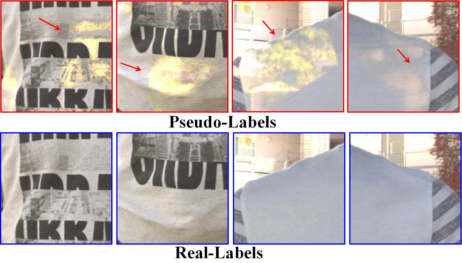
Pseudo-labels Selection Strategy. Since the sample-quality-based pseudo-labels selection strategy can exclude saturated and ghosted samples (see Figure 5), the model can be guided in a correct optimization direction which is effective for ghost removal. When we remove the pseudo-labels selection strategy, the performance of the model without APSS is dropped.

Two Stages Strategy. In Table 3, we report the performance of AHDR^∗. It achieves a significant increment compared with the vanilla AHDR model, which demonstrates the effectiveness of the overall two stages strategy.

Proposed Model Architecture. When we replace our two stages strategy with the FSHDR strategy, the numerical results increase compared with FSHDR. It shows that our proposed model architecture is also sound.

References

- [1] Sagie Benaim and Lior Wolf. One-shot unsupervised cross domain translation. Advances in neural information processing systems (NIPS), 31, 2018.
- [2] Luca Bertinetto, João F Henriques, Jack Valmadre, Philip Torr, and Andrea Vedaldi. Learning feed-forward one-shot learners. Advances in neural information processing systems (NIPS), 29, 2016.
- [3] L. Bogoni. Extending dynamic range of mono-chrome and color images through fusion. In IEEE International Conference on Pattern Recognition (ICPR), pages 7–12, 2000.
- [4] Chelsea Finn, Pieter Abbeel, and Sergey Levine. Model-agnostic meta-learning for fast adaptation of deep networks. In International conference on machine learning (ICML), pages 1126–1135. PMLR, 2017.
- [5] Thorsten Grosch. Fast and robust high dynamic range image generation with camera and object movement. In IEEE Conference of Vision , Modeling and Visualization (VMV), 2006.
- [6] Kaiming He, Xinlei Chen, Saining Xie, Yanghao Li, Piotr Dollár, and Ross Girshick. Masked autoencoders are scalable vision learners. In Proceedings of the IEEE/CVF Conference on Computer Vision and Pattern Recognition (CVPR), pages 16000–16009, 2022.
- [7] Jinhan Hu, Gyeongmin Choe, Zeeshan Nadir, Osama Nabil, Seok-Jun Lee, Hamid Sheikh, Youngjun Yoo, and Michael Polley. Sensor-realistic synthetic data engine for multi-frame high dynamic range photography. In Proceedings of the IEEE/CVF Conference on Computer Vision and Pattern Recognition (CVPR) Workshops, pages 516–517, 2020.
- [8] Jun Hu, O. Gallo, K. Pulli, and Xiaobai Sun. HDR deghosting: How to deal with saturation? In Proceedings of the IEEE/CVF Conference on Computer Vision and Pattern Recognition (CVPR), pages 1163–1170, 2013.
- [9] Nima Khademi Kalantari and Ravi Ramamoorthi. Deep high dynamic range imaging of dynamic scenes. ACM Transactions on Graphics, 36(4):1–12, 2017.
- [10] S. B. Kang, M. Uyttendaele, S. Winder, and R. Szeliski. High dynamic range video. ACM Transactions on Graphics, 22(3):319–325, 2003.
- [11] Chul Lee, Yuelong Li, and Vishal Monga. Ghost-free high dynamic range imaging via rank minimization. IEEE signal processing letters, 21(9):1045–1049, 2014.
- [12] Yoonho Lee and Seungjin Choi. Gradient-based meta-learning with learned layerwise metric and subspace. In International Conference on Machine Learning (ICML), pages 2927–2936. PMLR, 2018.
- [13] Jingyun Liang, Jiezhang Cao, Guolei Sun, Kai Zhang, Luc Van Gool, and Radu Timofte. Swinir: Image restoration using swin transformer. In Proceedings of the IEEE/CVF International Conference on Computer Vision (ICCV) Workshops, pages 1833–1844, 2021.
- [14] Zhen Liu, Lin Wenjie, Li Xinpeng, Rao Qing, Jiang Ting, Han Mingyan, Fan Haoqiang, Sun Jian, and Liu Shuaicheng. Adnet: Attention-guided deformable convolutional network for high dynamic range imaging. In Proceedings of the IEEE/CVF Conference on Computer Vision and Pattern Recognition (CVPR) Workshops, pages 463–470, 2021.
- [15] Kede Ma, Li Hui, Yong Hongwei, Wang Zhou, Meng Deyu, and Zhang. Lei. Robust multi-exposure image fusion: A structural patch decomposition approach. IEEE Transactions on Image Processing, 26(5):2519–2532, 2017.
- [16] Rafat Mantiuk, Kil Joong Kim, Allan G. Rempel, and Wolfgang Heidrich. HDR-VDP-2:a calibrated visual metric for visibility and quality predictions in all luminance conditions. In ACM Siggraph, pages 1–14, 2011.
- [17] Alexander Miller, Adam Fisch, Jesse Dodge, Amir-Hossein Karimi, Antoine Bordes, and Jason Weston. Key-value memory networks for directly reading documents. arXiv preprint arXiv:1606.03126, 2016.
- [18] Yuzhen Niu, Wu Jianbin, Liu Wenxi, Guo Wenzhong, and WH Lau. Rynson. Hdr-gan: Hdr image reconstruction from multi-exposed ldr images with large motions. IEEE Transactions on Image Processing, 30:3885–3896, 2021.
- [19] Tae-Hyun Oh, Joon-Young Lee, Yu-Wing Tai, and In So Kweon. Robust high dynamic range imaging by rank minimization. IEEE Transactions on Pattern Analysis and Machine Intelligence, 37(6):1219–1232, 2015.
- [20] Fabrizio Pece and Jan Kautz. Bitmap movement detection: HDR for dynamic scenes. In Visual Media Production (CVMP), pages 1–8, 2010.
- [21] K Ram Prabhakar, Rajat Arora, Adhitya Swaminathan, Kunal Pratap Singh, and R Venkatesh Babu. A fast, scalable, and reliable deghosting method for extreme exposure fusion. In 2019 IEEE International Conference on Computational Photography (ICCP), pages 1–8. IEEE, 2019.
- [22] K Ram Prabhakar, Gowtham Senthil, Susmit Agrawal, R Venkatesh Babu, and Rama Krishna Sai S Gorthi. Labeled from unlabeled: Exploiting unlabeled data for few-shot deep hdr deghosting. In Proceedings of the IEEE/CVF Conference on Computer Vision and Pattern Recognition (CVPR), pages 4875–4885, 2021.
- [23] Hang Qi, Matthew Brown, and David G Lowe. Low-shot learning with imprinted weights. In Proceedings of the IEEE/CVF Conference on Computer Vision and Pattern Recognition (CVPR), pages 5822–5830, 2018.
- [24] Pradeep Sen, Khademi Kalantari Nima, Yaesoubi Maziar, Darabi Soheil, Dan B Goldman, and Eli Shechtman. Robust patch-based HDR reconstruction of dynamic scenes. ACM Transactions on Graphics, 31(6):1–11, 2012.
- [25] Pranav Shyam, Shubham Gupta, and Ambedkar Dukkipati. Attentive recurrent comparators. In International conference on machine learning (ICML), pages 3173–3181. PMLR, 2017.
- [26] Sainbayar Sukhbaatar, Jason Weston, Rob Fergus, et al. End-to-end memory networks. Advances in neural information processing systems (NIPS), 28, 2015.
- [27] Anna Tomaszewska and Radoslaw Mantiuk. Image registration for multi-exposure high dynamic range image acquisition. In International Conference in Central Europe on Computer Graphics and Visualization (WSCG), 2007.
- [28] Okan Tarhan Tursun, Ahmet Oğuz Akyüz, Aykut Erdem, and Erkut Erdem. An objective deghosting quality metric for HDR images. Comput. Graph. Forum, 35(2):139–152, 2016.
- [29] Xintao Wang, Kelvin CK Chan, Ke Yu, Chao Dong, and Chen Change Loy. Edvr: Video restoration with enhanced deformable convolutional networks. In Proceedings of the IEEE/CVF Conference on Computer Vision and Pattern Recognition (CVPR) Workshops, pages 0–0, 2019.
- [30] Shangzhe Wu, Xu Jiarui, Tai Yu-Wing, and Tang. Chi-Keung. Deep high dynamic range imaging with large foreground motions. In Proceedings of the European Conference on Computer Vision (ECCV), pages 117–132, 2018.
- [31] Qingsen Yan, Gong Dong, Shi Qinfeng, van den Hengel Anton, Shen Chunhua, Reid Ian, and Zhang Yanning. Attention-guided network for ghost-free high dynamic range imaging. In Proceedings of the IEEE/CVF Conference on Computer Vision and Pattern Recognition (CVPR), pages 1751–1760, 2019.
- [32] Qingsen Yan, Dong Gong, Javen Qinfeng Shi, Anton van den Hengel, Chunhua Shen, Ian Reid, and Yanning Zhang. Dual-attention-guided network for ghost-free high dynamic range imaging. International Journal of Computer Vision, 130(1):76–94, 2022.
- [33] Qingsen Yan, Dong Gong, Javen Qinfeng Shi, Anton van den Hengel, Jinqiu Sun, Yu Zhu, and Yanning Zhang. High dynamic range imaging via gradient-aware context aggregation network. Pattern Recognition, 122:108342, 2022.
- [34] Qingsen Yan, Zhang Lei, Liu Yu, Zhu Yu, Sun Jinqiu, Shi Qinfeng, and Zhang Yanning. Deep hdr imaging via a nonlocal network. IEEE Transactions on Image Processing, 29:4308–4322, 2020.
- [35] Qingsen Yan, Jinqiu Sun, Haisen Li, Yu Zhu, and Yanning Zhang. High dynamic range imaging by sparse representation. Neurocomputing, 269:160–169, 2017.
- [36] Qingsen Yan, Bo Wang, Peipei Li, Xianjun Li, Ao Zhang, Qinfeng Shi, Zheng You, Yu Zhu, Jinqiu Sun, and Yanning Zhang. Ghost removal via channel attention in exposure fusion. Computer Vision and Image Understanding, 201:103079, 2020.
- [37] Qingsen Yan, Yu Zhu, and Yanning Zhang. Robust artifact-free high dynamic range imaging of dynamic scenes. Multimedia Tools and Applications, 78:11487–11505, 2019.
- [38] Qian Ye, Jun Xiao, Kin-man Lam, and Takayuki Okatani. Progressive and selective fusion network for high dynamic range imaging. In Proceedings of the 29th ACM International Conference on Multimedia (ACM MM), pages 5290–5297, 2021.
- [39] Jaesik Yoon, Taesup Kim, Ousmane Dia, Sungwoong Kim, Yoshua Bengio, and Sungjin Ahn. Bayesian model-agnostic meta-learning. Advances in neural information processing systems (NIPS), 31, 2018.
- [40] Wei Zhang and Wai-Kuen Cham. Gradient-directed multiexposure composition. IEEE Transactions on Image Processing, 21(4):2318–2323, 2011.