online_appendix \newcitesAppendixAppendix References \WarningFilter*natbibCitation
Smartphone Data Reveal Neighborhood-Level Racial Disparities in Police Presence
While extensive, research on policing in America has focused on documented actions such as stops and arrests—less is known about patrolling and presence. We map the movements of over ten thousand police officers across twenty-one of America’s largest cities by combining anonymized smartphone data with station and precinct boundaries. Police spend considerably more time in Black neighborhoods, a disparity which persists after controlling for density, socioeconomics, and crime-driven demand for policing. Our results suggest that roughly half of observed racial disparities in arrests are associated with this exposure disparity, which is lower in cities with more supervisor (but not officer) diversity.
According to FBI statistics, in 2019 Black people in America were arrested at twice the rate of White people (OJJDP Statistical Briefing Book 2019). A large literature explores the causes of racial disparities in policing outcomes such as stops, searches, and arrests, including differences in socioeconomic status, criminal activity, and biased decision making by police officers (Banaji et al. 2021; Banks et al. 2006; Hoekstra and Sloan 2022; Rucker and Richeson 2021). We document and explore another potential factor: racial disparities in police presence.
The police wield considerable discretion in determining where, exactly, law enforcement is provided within America’s cities. Where officers are located has direct implications for the deterrence of potential criminals. It also affects what the broader public knows about crime, as police presence can influence when and where crime is officially observed and recorded. Finally, since police contact is the first part of any criminal justice involvement, and the racial composition of neighborhoods varies both across and within cities, detailed information on where officers work during their shifts can potentially identify sources of disparities in later criminal justice outcomes.
Unfortunately, few departments collect detailed officer location data, and even fewer release it to researchers in a standardized way. We use anonymized smartphone location data to identify and track the movements of individual police officers while on patrol. These data identify where police spend their time, and allow us to evaluate spatial patterns of policing at scale while protecting officer privacy. Using these data, we quantify how patterns of socioeconomic status, crime, social capital, and race relate to local police “presence” within and across twenty-one of America’s largest cities.
Generally, geographic analysis of policing at the sub-city level has measured local policing in two ways: “up-funnel” or “down-funnel” measurement. Like Ba et al. (2021); Vomfell and Stewart (2021); Mastrobuoni (2019) and Weisburd (2021), we use an “up-funnel” measurement approach, capturing information on where police conduct patrol. In contrast, “down-funnel” measures capture observed police enforcement actions that are made public by a department (e.g. use of force, arrests, or stops). We are able to build on existing up-funnel studies, as we can track exact officer location, rather than where officers are instructed to go.
We measure police presence as the total number of officer hours spent in a census block group (a “neighborhood” with roughly 1,000 residents) over a ten-month period (Feb 2017 - Nov 2017), when the officer was moving through a neighborhood at 50 mph or less. Comparisons of assigned officer beats, an alternative up-funnel measure used in, for example, Ba et al. (2021), with actual patrol car locations suggest that while beats are highly correlated with actual officer presence, officers spend a nontrivial amount of time outside of their officially assigned geographic locations (Weisburd 2021). Further, unlike studies based on Automatic Vehicle Location (AVL) technology, we are able to capture the time patrol officers spend patrolling outside of their cars. Finally, we are able to extend beyond a single-city analysis based on Automatic Vehicle Location (AVL) or assigned beat data to a much broader set of US cities by using smartphone GPS data that are broadly representative of the United States population (Long et al. 2020).
Our sub-city analysis of GPS location data confirms many hypotheses posed by qualitative and historical research on up-funnel police presence across America (Hinton 2016; Rios 2011; Sharkey 2018), and patterns observed at the city level (Carmichael and Kent 2014). For example, we show that police officers spend more time in places with larger Black, Hispanic, or Asian populations relative to the city overall. While controlling for neighborhood differences in socioeconomic status, social disorganization, and violent crime reduces these disparities, it does not eliminate them. This suggests that social interventions targeted at the “root causes” of crime may be unlikely to eliminate the racial disparities we observe in American policing.
Our up-funnel approach has distinct advantages over down-funnel approaches; enforcement-based measures of policing do not fully measure officer presence in a neighborhood - the most fundamental element of what it means for an area to be “policed,” and in particular fail to capture the extent to which police officers allocate time to the increasingly diverse set of tasks they perform within a community (Brooks 2021; Lum 2021; Lum et al. 2021). At the same time, our measure of officer presence complements existing spatial analyses of down-funnel, enforcement-based measures of policing by contributing analysis of pre-enforcement exposure to police at a highly granular level. For example, many studies have found that police engage in more enforcement actions in Black neighborhoods, with more mixed evidence in Hispanic neighborhoods (Geller et al. 2014; Ba et al. 2021; Pierson et al. 2020). Combining our police presence data with geocoded arrest data that are available for six cities (including New York City), our estimates suggest that in this sub-sample, differences in where officers spend time explain roughly 60% of the Black-White disparity, and almost 70% of the Hispanic-White disparity in arrests. Officers’ higher propensity to make an arrest, conditional on being in a non-White neighborhood, explains the remainder of these disparities.
While still descriptive, we also explore differences in police presence associated with the racial composition of front-line officers versus police supervisors across cities. Consistent with existing single-department studies (e.g. Hoekstra and Sloan 2022; Ba et al. 2021), our results suggest that the additional police presence in Black neighborhoods is lower in cities where more police officers are Black. However, this is not statistically explained by the racial composition of patrol officers walking the beat, but rather by the racial composition of the supervisors that direct patrol officer activity. While not causal, this highlights the potential role of retention and promotion in police reform aimed at reducing racial disparities in the criminal justice system. We then provide evidence that the nature of disparities in policing presence differs across US cities. While some disparities in some cities (e.g. Charlotte, NC) are largely associated with spatial differences in socioeconomic status (e.g., income, education, and civic engagement) others persist even when controlling for these factors, including spatial patterns of violent crime (e.g. Austin, TX).
Our findings suggest that disparities in exposure to police are associated with both structural socioeconomic disparities and discretionary decision making by police commanders and officers. Hence, this study provides novel data on police-civilian interaction to enable additional analyses of the factors driving these observed effects in hopes of developing policy interventions to mitigate them. Finally, our police presence measure provides a new benchmark against which down-funnel police actions like stops and arrests may be objectively evaluated.
2 Methods
2.1 Data
The smartphone location data used in this study were provided by Safegraph and can now be obtained from Veraset, a company that aggregates anonymized location data from a suite of smartphone applications. The smartphone data records “pings” denoting where a specific smartphone is located at a particular point in time. Pings are logged at irregular time intervals, whenever a participating smartphone application requests location information. The modal time between consecutive pings associated with a device is roughly 10 minutes. Our smartphone data covers more than 50 million smartphones, spanning the continental US, in a 10-month period from February 2017 to November 2017. While the dataset contains geolocation information from only a subset of all smartphones, previous studies have found it highly representative of the United States on numerous demographic dimensions (Long et al. 2020).
We link the smartphone data to two other data sources: 1) police station location data published by the Department of Homeland Security, verified with the city’s open data portal and google maps data, and 2) building rooftop geofence data provided by Microsoft, enabling us to associate each police station’s latitude-longitude location to a geofence that delineates the convex hull of a building’s rooftop boundary. To identify patrol officers in local city neighborhoods, we include police stations categorized as patrol stations, as headquarters, or as unspecified police facilities, resulting in a total of 330 stations across 21 of America’s largest cities. A description of other data sources and data cleaning process can be found in Appendix A1. It is important to note the selection of the cities in our sample was based on jurisdictional population and the physical construction of police buildings. Our sample was not determined by the investment the department chose to make in electronic monitoring of officers, or a department’s decision to release the data publicly or enter into a research agreements with external parties (see Goel et al. (2017) for a discussion of these issues in the context of measuring police bias).
2.2 Measuring Police Presence
We infer whether a smartphone belongs to an officer by linking smartphone data to police stations’ geofences in several steps. First, if a specific smartphone is observed in a police station geofence at least five days in a month, we identify it as belonging to a police employee in that month. We next infer each smartphone user’s “home” as the smartphone’s modal Geohash-7 (a 152m 152m grid) during a five-month period when the device is not at any police stations. We identify two home locations separately for the early and the latter half of the year to account for a potential summer move. Then, we identify patrol officers by looking for a specific pattern: leaving home, traveling to a police station, moving around the city (without returning home), returning to the police station, and then going home. The movements of that smartphone between the first and the last station visits are assumed to be the actual locations of a patrol officer while working a “shift.” We require that shifts are bracketed by home visits that are no more than 24 hours apart, and are no shorter than four hours.111All results in our analysis are highly robust to limiting our sample to 8 to 12 hour shifts, requiring shifts bracketed by home visits no longer than 18 hours and excluding shifts with long hours spent within the police stations. These results are available on request. Under this definition, our officer smartphone GPS data sample consists of 10,131 officers that have at least one shift, with the mean of shift lengths being 8.08 hours.222Figure LABEL:fig:mode in the Online Appendix displays the spatial pattern of pings for one likely LAPD officer.
To measure police presence in all census block groups (“neighborhoods”) within the city’s jurisdiction, we look at officers’ smartphone pings outside of the police stations when officers are “on shift” in the month where the device has at least 5 days’ presence. We conceptualize police presence in a city neighborhood as the number of officer-hours spent in the neighborhood. Specifically, we match police officers’ ping locations to block groups, exclude pings moving faster than 50 mph, and assign the duration of each ping as half of the time between its previous and next ping.333Using other constructs of police presence yields qualitatively and quantitatively similar results. Replications of our analysis using the number of distinct officer shifts, alternate (or no) speed thresholds, and alternate lengths of shifts or time between home visits are available on request. We then compute the sum of officer-hours from all officers’ pings observed in the block group as police hours across the ten-month period. Where police spend time on patrol is highly non-uniform, and as our later regression analysis will confirm, is strongly correlated with demographics in ways that produce large racial disparities.
2.3 Validity Check
Our study focuses on America’s largest cities. While our data do not capture the universe of police officers in a city, our estimates of the number of officers in a city satisfy many tests of face validity as a measure of police presence. The number of officer devices that we observe across US cities is highly correlated with FBI estimates of police force size ( = 0.98 for total count measures, = 0.64 for per capita measures).444Appendix Figure LABEL:fig:officers_count plots the specific values for each city. Further, we can probabilistically impute each device’s “race” using its home census block’s racial composition to estimate each police department’s racial composition. There is essentially a one for one unconditional relationship between the imputed race of the police departments in our sample and the racial composition reported by the department in the 2016 Law Enforcement Management and Administration Statistics (LEMAS); conditional on the racial composition of the city, a one percentage point increase in our estimate of the percent of the police force that is White (Black, Hispanic, Asian) is associated with a 0.6 (0.5, 0.9, 0.6) percentage point increase in the reported percent of the force that is White (Black, Hispanic, Asian) in the LEMAS. 555Appendix Figure LABEL:fig:LEMAS_compare plots the raw data. The p-value testing whether the slope between the smartphone GPS measures and LEMAS measure of racial composition is equal to 1 is 0.946 for Black, 0.890 for White, and 0.099 for Hispanic. The slopes between the two estimates for the share of Asian is significantly different from 1, though Asians account for only 2.5% of the police force across the cities in LEMAS. Table LABEL:tab:LEMAS in the Appendix further shows that this significant correlation is not simply driven by cross-city variation in racial composition.
We conduct an additional residence-based validity check in New York City, in which public records provide summary data on where NYPD officers live at the zip code level. We compare the NYPD’s official records on the number of officers who live in a zip code with the number of officers that our smartphone GPS measures estimate “live” in that zip code. There is a strong and positive correlation ( = 0.71) between official NYPD records and our smartphone-based measures.666Figure LABEL:fig:NYPD_counts in the Appendix plots the zip code level data.
There is a well-established positive correlation between the fraction of a city population that is Black and the number of sworn police officers per capita (Carmichael and Kent 2014; Stults and Baumer 2007). A basic test of construct validity is therefore to test if we observe a similar pattern in our data. Figure 1 plots per capita patrol officers (i.e. smartphones that have at least one shift) against the share of Black population in the 21 cities, replicating the positive correlation between the fraction of city residents who are Black and our measure of total officers per capita. Our GPS-based measure of police presence has significant predictive power on down-funnel measures of police actions, such as stops and arrests. After adjusting for nonlinearity, the correlation between our measure of police presence and the number of arrests—which we observe in six cities—ranges from 0.46 (Washington) to 0.68 (Austin). Similar positive and significant correlations for police stops for nine cities with publicly available geocoded records on police stops are observed. 777Appendix Figures LABEL:fig:arrests and LABEL:fig:stops plot these city by city graphs.
3 Results
3.1 Neighborhood Correlates of Police Presence
Understanding how police provide services to people from different racial groups is important from both an equity and an efficiency perspective, and our data are uniquely suited to provide new evidence on this issue. Within each neighborhood, we measure the concentration of different racial/ethnic groups as the ratio of the percent of neighborhood residents who report being in a particular category divided by the percent of city residents who report the same. This reflects the observation that exactly what constitutes a “more” Asian, Black, or Hispanic neighborhood is likely different in Detroit than in San Francisco. One convenient feature of our relative share measure is that one unit increase relative to the mean roughly corresponds to a neighborhood with twice as many Asian, Black, or Hispanic residents as in the city as a whole. Table LABEL:tab:sumstat in the Appendix shows summary statistics for police presence measures as well as neighborhood correlates.888Results measuring racial share in an absolute way, or using a series of dummies to indicate that the majority of residents identify themselves as a particular group are qualitatively identical, and available on request.
Table 1 presents our estimates of the spatial determinates of policing in America’s largest cities. Our smartphone GPS data reveal a strong relationship between the racial and ethnic composition of a neighborhood and police presence. Relative to the average city neighborhood, our coefficients in Table 1 suggest police spend 8.2% more time in a place where the fraction of residents who are Black is twice the city’s share, 5.2% more time in a place with twice the share of Hispanic residents, and 1.4% more time in a place where twice as many neighborhood residents are Asian as in their respective city as a whole.999The elasticity for a arsinh-transformed is , hence for Black concentration, the calculation of the elasticity is 1.0007*1.023*0.0801 = 8.2%, for Hispanic concentration, the elasticity is 1.0007*0.944*0.0554 5.2%, and for Asian concentration, the elasticity is 1.0007*0.895*0.0155 = 1.4%.
Why do these disparities exist? Differences in where police spend their time can reflect decisions made by individual officers and department-level directives, both of which involve assessing the “need” for police presence in an area. Such department policies, officer decisions, and residential demand for police presence can all be related to the racial composition of the neighborhood. We use a multivariate regression framework to provide insight into why police may tend to spend more time in places with relatively more Asian, Black, and Hispanic residents.
We begin by introducing proxies for residential demand. If officers spend more time in places where there are more people, variation in population density that is correlated with race may contribute to spatial differences in policing. Location decisions can also indicate residential demand for police presence. Residents may request that officers respond to crimes, and in particularly disadvantaged neighborhoods, police officers may be one of the few remaining providers of any social service (Lum 2021). Racial disparities in police presence may therefore stem from racial inequity in the quality of non-policing institutions.
We draw on existing social science literature to approximate components of civilian demand for police. A lack of educational opportunity and well-paying jobs are established root causes of crime (Messner and Rosenfeld 1997). Of course, neighborhoods where residents have low incomes but high social capital (e.g. high degrees of social cohesion and community engagement) are places where police rarely need to respond to acts of violence or property destruction (Sampson and Raudenbush 1999). Following Martin and Newman (2015), we measure social capital using the fraction of 2010 census forms returned by residents. Finally, police officers go where violent crime exists. We estimate the crime-driven demand for police based on the location of homicides known to the police. While imperfect and sparse, police records of homicides are generally thought to be the most accurate, in the sense that reporting of homicides is unlikely to be as influenced by police presence as reporting of other types of crime (Levitt 1998). We calculate the distance from the neighborhood center to the closest homicide in 2016, treating these rare events as an extreme expression of underlying social issues, implicitly assuming that this distance is negatively correlated with exposure to other types of crime. Additionally, we control for the number of homicides in 2016, by neighborhood, to account for potential high-end variation in crime.
Alternate measures of demand for policing, specifically using additional years of homicide data and 311 calls for service in New York City (Shah and LaForest 2021) are explored in the Online Appendix - none lead to substantively different conclusions. We also compare how police presence varies with residential composition when we exclude times of day, and places, where the modal person on the street may not live there. In the Online Appendix, we show that our findings are qualitatively identical when we model police presence during non-working hours (excluding 9 am - 5 pm), and in New York City when we exclude census block groups in tourist destinations. Finally, we show that the relationship between exposure to police presence and the relative composition of the block group that is Black or Hispanic is highest during the middle of an officer’s shift.
In column 2 of Table 1, we condition our estimates of local police presence in different types of U.S. neighborhoods on measures of density, socioeconomics, social cohesion, and violence. Differential residential demand for police presence, some of which is created by decisions made in other policy domains, explains approximately 26% of the disparate exposure of people living in relatively Black neighborhoods, 42% of the disparate exposure of people living in relatively Hispanic neighborhoods, and can explain all of the additional exposure of people living in relatively Asian neighborhoods—even suggesting that more Asian neighborhoods have less police presence than one might expect based on social conditions. The residual correlation between racial composition and police presence in column 2 reflects decisions at the city, police command, and officer level.
In column 3, we include city-specific fixed effects, differencing out any preference of officials in cities with more concentrated non-White populations for a particular type of policing that may contribute to observed disparities in policing. Focusing on variation in neighborhoods within cities reduces the estimated extra time officers spend in more relatively Black neighborhoods by an additional 60%, and reduces the lighter policing of more Asian neighborhoods by 11%. Across large cities, officers spend more time in neighborhoods with relatively more Hispanic people, but we do not observe this pattern within cities.
Diversifying the officer ranks is one city-level policy that is central to many police reform efforts. With this in mind, we compare how disparities in police presence vary with the racial composition of a city’s police force. We do this in two ways: including the mean-centered interaction between the relative share of Black residents and the share of police officers that are Black in column 4, and interactions with both the share of police supervisors and patrol officers that are Black in column 5.101010Appendix Figure LABEL:fig:supervisor reveals substantial variation in the Black share in police officers and supervisors relative to the city’s Black population across cities, and a meaningful difference between the share of Black officers and supervisors, despite a high correlation between the two measures. Both departmental measures are divided by the share of the city that is Black. Column 4 suggests the additional exposure to police in Black neighborhoods is smaller in cities with a larger share of Black officers. Column 5 implies that conditional on the composition of patrol officers, when the share of Black command staff is higher, there is less additional police presence in Black neighborhoods. In contrast to previous studies (e.g. Ba et al. 2021), conditional on the share of command that is Black, we find that jurisdictions that employ more Black officers are also jurisdictions with more exposure of people in Black neighborhoods to police, both across and within cities (Column 6). While correlational in nature, our findings suggest that efforts to hire more Black police officers, without parallel efforts to retain and promote those officers, may not reduce disparities in how the public is policed.
3.2 Cross-city variation in correlates of police presence
Our findings suggest substantial differences in the level of ambient police presence in non-White neighborhoods across the United States, and this difference is largest in Black neighborhoods. Given this, and the long and fraught history of the policing of Black people in the United States, in this section we report the difference in 2017 police presence in neighborhoods with the highest concentrations of Black residents and highest concentrations of White residents. First, in Figure 2, we show police presence in neighborhoods with the greatest concentration of Black and White residents, respectively, to highlight the range of disparities in Black-White neighborhood policing across major US cities. There is little difference in the amount of time that police spend in the “most White” and “most Black” neighborhoods in Boston, but over 100 more hours of total policing in the “most Black” neighborhoods in Charlotte than in the “most White.”
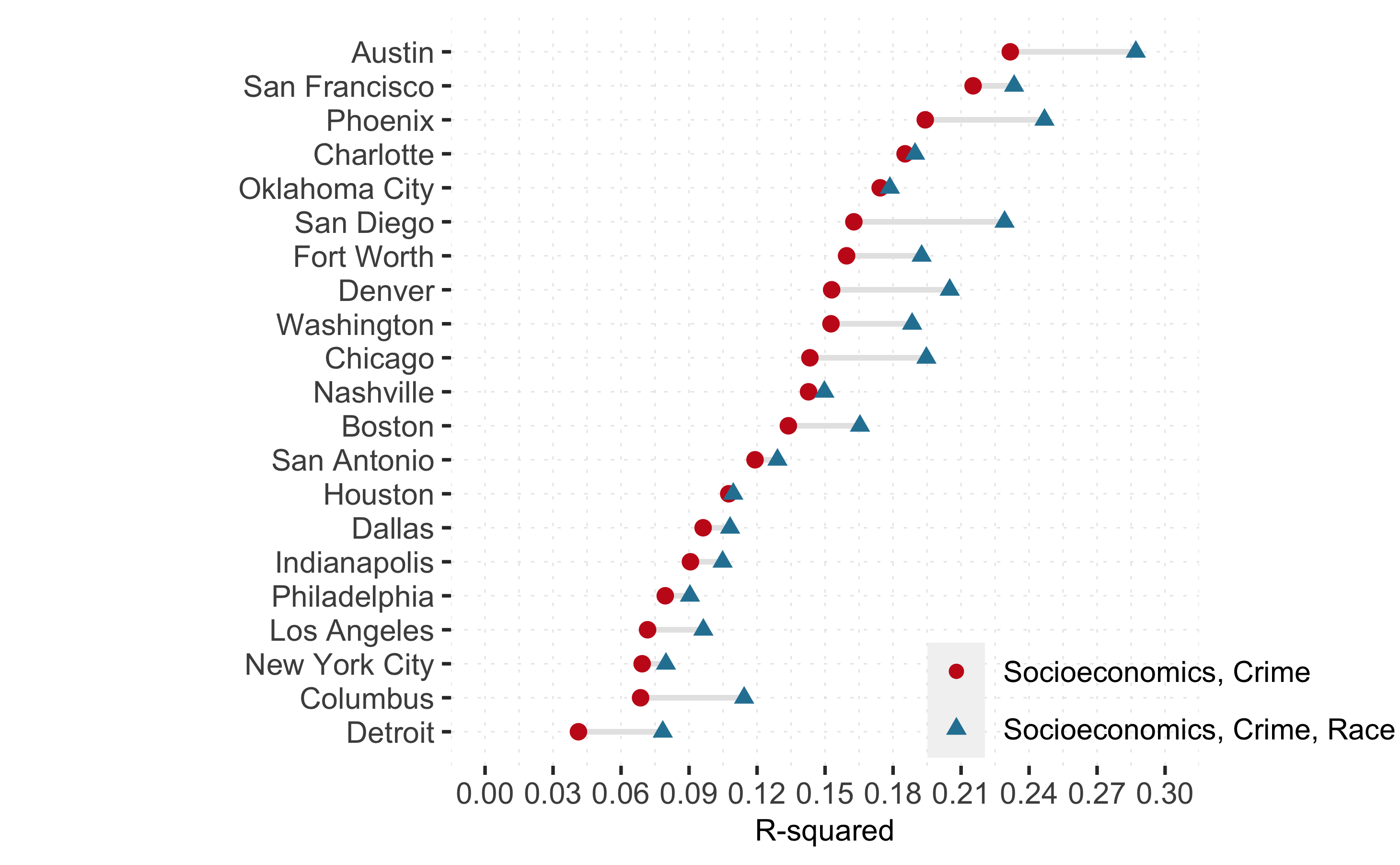
Of course, these disparities can have many sources. In Figure 3, we plot, for each city, how much of the spatial variation in police presence can be explained by spatial variation in our proxies for “demand” for police, and how much the explanatory power of our models increases when we add controls for relative racial composition. This shows the extent to which Black-White disparities in exposure to police can persist even when considering spatial differences in socioeconomic status - which in some cases may reflect historical and contemporary race-based social and economic inequality. We document substantial variation across cities in the role of this structural inequality in explaining policing disparities. For example, while Figure 2 reveals large differences in the ambient police exposure of Black and White Charlotte residents, Figure 3 reveals that spatial disparities in socioeconomic status explain almost all of these differences. These structural disparities in Charlotte are city-level issues that cannot be addressed solely by the city’s police department. In contrast, racial disparities in police presence are absolutely smaller in Austin, but incorporating Black, Hispanic, and Asian residential patterns increases the amount of spatial variation in police presence that we can explain in that city by 27%. This suggests substantially more scope for changes in police policy to reduce criminal justice disparities in Austin, TX.
3.3 Using Police Presence to Understand Police Enforcement
The empirical observation that police are more ambiently present in Non-White neighborhoods provides support for the construct validity of our data, as this correlation has been repeatedly demonstrated at the city level (Carmichael and Kent 2014). When taken in the context of existing qualitative and legal scholarship on modern policing, this also raises equity concerns.
Past research highlights how the increased use of surveillance (either remotely or in-person) by law enforcement and algorithmic policing can reinforce existing racial disparities, even in the absence of differential criminal behavior by residents (Ba et al. 2021; Brayne 2020). Our measure of police presence can quantify the extent to which variation in ambient police presence, rather than differences in the enforcement behavior of officers in different neighborhood contexts, can predict racial disparities in police enforcement.
Consistent with studies of down-funnel measures of policing, Table 2 confirms that in the six cities (New York City, Los Angeles, Chicago, Dallas, Austin, Washington) for which we have both police presence and arrest data, officers spend more time, and make more arrests in places with higher relative Black shares. Note that the Black-White disparity in police presence is 27% smaller, the Hispanic-White disparity 20% smaller, and the Asian-White disparity 165% larger, in this sub-sample of cities that make geocoded arrest data public. In addition, officers appear to make almost 24% more arrests per hour present in neighborhoods where the share of residents who are Black is twice the city’s share.111111In contrast to our findings regarding the source of Black-White arrest disparities, smartphone data do not suggest that differences in police presence are an important source of Hispanic-White arrest disparities. This could be due to Becker-style discrimination, where police use different standards to determine if people in different groups are suspicious enough to warrant an arrest, or to differences in where police officers spend time in these neighborhoods.121212This type of Becker-style discrimination is not necessarily illegal; Illinois v Wardlow, 528 U. S. 119 (2000) established that officers can use the predetermined designation of an area as “high crime” in determining how likely it is someone has (or is) engaged in crime, creating a legal basis for a stop. If places with more Black or Hispanic residents are more likely to be known to police as “high crime” places, then this would lower the standard of individualized suspicion needed to make a constitutionally permissible stop. Whatever the source, this disparity in the propensity of an officer to make an arrest explains less than half of the disparity in the total number of arrests made. This implies that the added time that police spend in Black neighborhoods may be a central source of Black-White disparities in arrests, in addition to an officer’s decision in a particular encounter. Online Appendix Table LABEL:tab:stop also reveals a highly similar pattern regarding stop disparities. Consistent with Meares (2015), our results suggest that, to reduce disparities in criminal justice, reducing the scope for racial bias both in specific civilian encounters and in police directives detailing where officers go and who they surveil may be warranted.
4 Conclusion
We conclude by noting that a positive correlation in the provision of policing and the concentration of Black residents contrasts with documented spatial patterns of other institutional investment in neighborhoods with concentrated Black populations. Census tracts where more of the residential population is Black are less, not more, likely to have a large grocery store, nearby hospital, or local banking services (Walker et al. 2010, DeYoung et al. 2008, Lieberman-Cribbin et al. 2020, Yearby 2018). During the 2016 election, Chen et al. (2019) found that voting lines moved more slowly in places with larger Black populations, suggesting under-investment in polling services in places where we observe larger investments in ambient policing.
Our data are well suited to further research on policing in the United States. First, smartphone location data provide insight into officer presence in communities that traditional measures of policing cannot fully capture. Measuring officer presence informs estimates of which communities are at risk of more serious police encounters, like arrest or the use of lethal force. Second, our smartphone location data do not depend on software purchased by or developed for a particular policing agency, allowing us to map officer locations in cities across the United States using a consistent methodology. This is an advantage over technologies like AVL and body cameras, because it provides enhanced visibility into the unreported and highly discretionary activities of police officers at work. Finally, data on where officers actually spend their time grants researchers and practitioners new abilities to understand patterns in police presence and track the implementation of departmental policies that shape the provision of public safety. Thereby, our data may serve as a baseline measure to objectively evaluate the intensity of down-funnel police actions like stops and arrests within neighborhoods across major U.S. cities.
References
- (1)
- Ba et al. (2021) Ba, Bocar A., Dean Knox, Jonathan Mummolo, and Roman Rivera (2021) “The role of officer race and gender in police-civilian interactions in Chicago,” Science, 371 (6530), 696–702.
- Banaji et al. (2021) Banaji, Mahzarin R, Susan T Fiske, and Douglas S Massey (2021) “Systemic racism: individuals and interactions, institutions and society,” Cognitive research: principles and implications, 6 (1), 1–21.
- Banks et al. (2006) Banks, R Richard, Jennifer L Eberhardt, and Lee Ross (2006) “Discrimination and implicit bias in a racially unequal society,” California Law Review, 94 (4), 1169–1190.
- Brayne (2020) Brayne, Sarah (2020) Predict and surveil: Data, discretion, and the future of policing: Oxford University Press, USA.
- Brooks (2021) Brooks, Rosa (2021) Tangled Up in Blue: Policing the American City: Penguin Press.
- Carmichael and Kent (2014) Carmichael, Jason and Stephanie Kent (2014) “The persistent significance of racial and economic inequality on the size of municipal police forces in the United States, 1980–2010,” Social Problems, 61, 259–282.
- Chen et al. (2019) Chen, M Keith, Kareem Haggag, Devin G Pope, and Ryne Rohla (2019) “Racial disparities in voting wait times: evidence from smartphone data,” Review of Economics and Statistics, 1–27.
- DeYoung et al. (2008) DeYoung, Robert, W Scott Frame, Dennis Glennon, Daniel P McMillen, and Peter Nigro (2008) “Commercial lending distance and historically underserved areas,” Journal of Economics and Business, 60 (1-2), 149–164.
- Geller et al. (2014) Geller, Amanda, Jeffrey Fagan, Tom Tyler, and Bruce G. Link (2014) “Aggressive Policing and the Mental Health of Young Urban Men,” American Journal of Public Health, 104 (12), 2321–2327.
- Goel et al. (2017) Goel, Sharad, Maya Perelman, Ravi Shroff, and David Sklansky (2017) “Combatting Police Discrimination in the Age of Big Data,” New Criminal Law Review: An International and Interdisciplinary Journal, 20, 181–232, 10.1525/nclr.2017.20.2.181.
- Hinton (2016) Hinton, Elizabeth (2016) From the War on Poverty to the War on Crime: The Making of Mass Incarceration in America: Harvard University Press.
- Hoekstra and Sloan (2022) Hoekstra, Mark and CarlyWill Sloan (2022) “Does Race Matter for Police Use of Force? Evidence from 911 Calls,” forthcoming, American Economic Review.
- Levitt (1998) Levitt, Steven D (1998) “The relationship between crime reporting and police: Implications for the use of Uniform Crime Reports,” Journal of Quantitative Criminology, 14 (1), 61–81.
- Lieberman-Cribbin et al. (2020) Lieberman-Cribbin, Wil, Stephanie Tuminello, Raja M Flores, and Emanuela Taioli (2020) “Disparities in COVID-19 testing and positivity in New York City,” American Journal of Preventive Medicine, 59 (3), 326–332.
- Long et al. (2020) Long, Elisa F, M Keith Chen, and Ryne Rohla (2020) “Political storms: Emergent partisan skepticism of hurricane risks,” Science Advances, 6 (37), eabb7906.
- Lum (2021) Lum, Cynthia (2021) “Perspectives on Policing,” Annual Review of Criminology, 4, 19–25.
- Lum et al. (2021) Lum, Cynthia, Christopher S. Koper, and Xiaoyun Wu (2021) “Can We Really Defund the Police? A Nine-Agency Study of Police Response to Calls for Service,” Police Quarterly, 10.1177/10986111211035002.
- Martin and Newman (2015) Martin, David C and Benjamin J Newman (2015) “Measuring aggregate social capital using census response rates,” American Politics Research, 43 (4), 625–642.
- Mastrobuoni (2019) Mastrobuoni, Giovanni (2019) “Police disruption and performance: Evidence from recurrent redeployments within a city,” Journal of Public Economics, 176, 18–31.
- Meares (2015) Meares, Tracey L (2015) “Programming errors: Understanding the constitutionality of stop-and-frisk as a program, not an incident,” University of Chicago Law Review, 82, 159.
- Messner and Rosenfeld (1997) Messner, Steven F and Richard Rosenfeld (1997) “Political restraint of the market and levels of criminal homicide: A cross-national application of institutional-anomie theory,” Social Forces, 75 (4), 1393–1416.
- OJJDP Statistical Briefing Book (2019) OJJDP Statistical Briefing Book (2019) Estimated number of arrests by offense and race, https://www.ojjdp.gov/ojstatbb/crime/ucr.asp?table˙in=2.
- Pierson et al. (2020) Pierson, Emma, Camelia Simoiu, Jan Overgoor et al. (2020) “A large-scale analysis of racial disparities in police stops across the United States,” Nature Human Behaviour, 4 (7), 736–745.
- Rios (2011) Rios, Victor (2011) Punished: Policing the Lives of Black and Latino Boys: New York University Press.
- Rucker and Richeson (2021) Rucker, Julian M and Jennifer A Richeson (2021) “Toward an understanding of structural racism: Implications for criminal justice,” Science, 374 (6565), 286–290.
- Sampson and Raudenbush (1999) Sampson, Robert J and Stephen W Raudenbush (1999) “Systematic social observation of public spaces: A new look at disorder in urban neighborhoods,” American Journal of Sociology, 105 (3), 603–651.
- Shah and LaForest (2021) Shah, Anuj K. and Michael LaForest (2021) “Knowledge About Others Reduces One’s Own Sense of Anonymity,” Working Paper.
- Sharkey (2018) Sharkey, Patrick (2018) Uneasy Peace: The Great Crime Decline, the Renewal of City Life, and the Next War on Violence: W. W. Norton and Company.
- Stults and Baumer (2007) Stults, Brian J and Eric P Baumer (2007) “Racial context and police force size: Evaluating the empirical validity of the minority threat perspective,” American Journal of Sociology, 113 (2), 507–546.
- Vomfell and Stewart (2021) Vomfell, Lara and Neil Stewart (2021) “Officer bias, over-patrolling and ethnic disparities in stop and search,” Nature Human Behaviour, 5 (5), 566–575.
- Walker et al. (2010) Walker, Renee E, Christopher R Keane, and Jessica G Burke (2010) “Disparities and access to healthy food in the United States: A review of food deserts literature,” Health & Place, 16 (5), 876–884.
- Weisburd (2021) Weisburd, Sarit (2021) “Police presence, rapid response rates, and crime prevention,” Review of Economics and Statistics, 103 (2), 280–293.
- Yearby (2018) Yearby, Ruqaiijah (2018) “Racial disparities in health status and access to healthcare: the continuation of inequality in the United States due to structural racism,” American Journal of Economics and Sociology, 77 (3-4), 1113–1152.
Figures and Tables
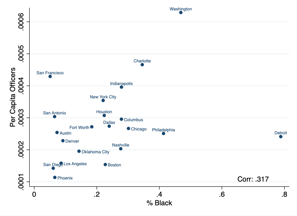
Notes: Per capita officers is defined as the number of likely patrol officers on “shift” divided by the city population. We identify patrol officers on “shift” by looking for a specific pattern in smartphones that visit at least 5 days in a month: Leaving “home”, traveling to a police station, moving around the city (without returning home), returning to the police station, and then going home. The correlation coefficient between the two measures is reported.
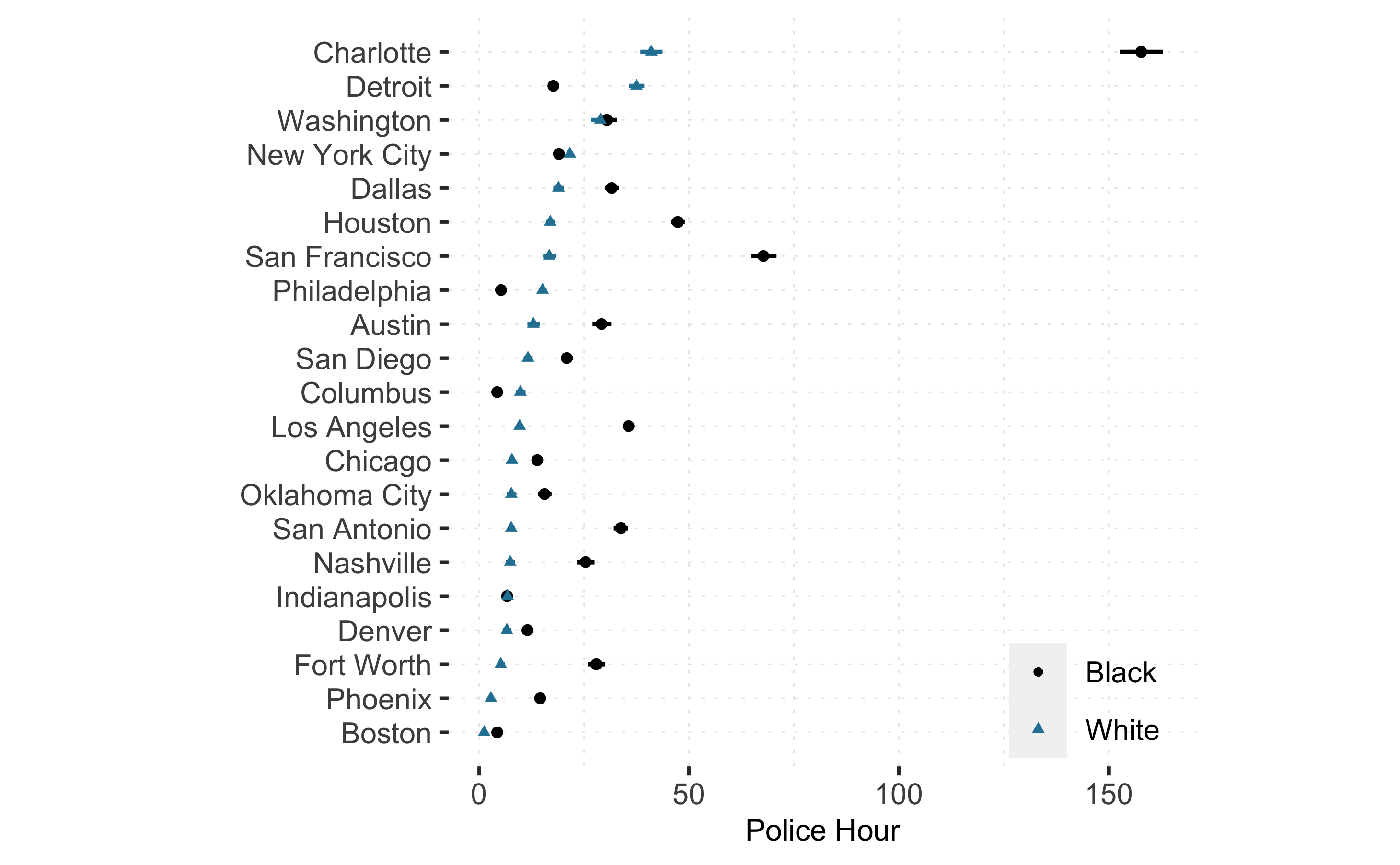
Notes: This figure plots the average police hours observed in the Blackest (Whitest) neighborhoods in a city, defined as the block groups where share of Black (White) residents is over the 95th percentile of the city’s distribution.
Notes: Socioeconomic variables include Log Population, % College Graduates, Median Household Income, Census Form Return Rate, Crime variables include Distance to Nearest Homicide and Homicide Count in 2016. Race variables include relative Black share, relative Hispanic share, and relative Asian share, defined as the ratio of percent Black (Hispanic, Asian) in the block group to percent Black (Hispanic, Asian) in the city.
| (1) | (2) | (3) | (4) | (5) | (6) | |
|---|---|---|---|---|---|---|
| VARIABLES | Police Exposure in a Census Block Group: arsinh(Hours) | |||||
| Relative Black Share | 0.0801*** | 0.0596*** | 0.0235** | 0.0543*** | 0.0713*** | 0.0398*** |
| (0.00731) | (0.00814) | (0.00794) | (0.00857) | (0.00904) | (0.00895) | |
| Police: Relative Black | 0.361*** | -0.734*** | ||||
| (0.0338) | (0.0795) | |||||
| Relative Black Share X Police: Relative Black | -0.0446+ | 0.158** | 0.160** | |||
| (0.0230) | (0.0563) | (0.0530) | ||||
| Supervisor: Relative Black | 0.648*** | |||||
| (0.0407) | ||||||
| Relative Black Share X Supervisor: Relative Black | -0.118*** | -0.102*** | ||||
| (0.0282) | (0.0267) | |||||
| Relative Hispanic Share | 0.0554*** | 0.0320** | -0.00977 | 0.0153 | 0.0311* | -0.000532 |
| (0.00999) | (0.0116) | (0.0104) | (0.0118) | (0.0121) | (0.0112) | |
| Relative Asian Share | 0.0155* | -0.0239*** | -0.0213*** | -0.0264*** | -0.0168* | -0.0159* |
| (0.00748) | (0.00607) | (0.00584) | (0.00635) | (0.00678) | (0.00645) | |
| Log Population | 0.540*** | 0.426*** | 0.548*** | 0.563*** | 0.455*** | |
| (0.0211) | (0.0212) | (0.0219) | (0.0223) | (0.0226) | ||
| % College Graduates | 1.083*** | 0.918*** | 1.036*** | 1.226*** | 1.042*** | |
| (0.0615) | (0.0602) | (0.0629) | (0.0640) | (0.0633) | ||
| Median Household Income (1K) | -0.00425*** | -0.00452*** | -0.00510*** | -0.00469*** | -0.00424*** | |
| (0.000394) | (0.000395) | (0.000405) | (0.000407) | (0.000408) | ||
| Census Form Return Rate | -0.635*** | -1.343*** | -0.446*** | -0.723*** | -1.400*** | |
| (0.125) | (0.127) | (0.131) | (0.134) | (0.137) | ||
| Distance to nearest 2016 homicide (km) | -0.0983*** | -0.125*** | -0.0718*** | -0.0808*** | -0.114*** | |
| (0.00624) | (0.00660) | (0.00657) | (0.00718) | (0.00755) | ||
| Homicide Count 2016 | 0.200*** | 0.205*** | 0.214*** | 0.224*** | 0.207*** | |
| (0.0206) | (0.0200) | (0.0212) | (0.0215) | (0.0212) | ||
| Observations | 23,682 | 22,521 | 22,521 | 20,961 | 20,112 | 20,112 |
| R-squared | 0.005 | 0.069 | 0.166 | 0.073 | 0.090 | 0.157 |
| Fixed effects | NA | NA | City | NA | NA | City |
Notes: This table presents OLS estimates of exposure disparities among census block groups (BGs) across (Column 1,2,4,5) and within 21 large cities (Column 3, 6). All race variables are mean-centered, relative Black (Hispanic, Asian) shares are defined as the ratio of % Black (Hispanic, Asian) in a BG to the % in that city, Police (Supervisor) Relative Black defined as the ratio of % Black of a department’s sworn officers (supervisors) to the % in that city. The dependent variable is police hours observed in a BG (excluding pings moving faster than 50 mph), transformed into arsinh values. Household income is measured in thousands of dollars, census return rates range from 0-1. Robust standard errors are reported in parentheses, and standard errors clustered at the tract level are reported in the SI Appendix. Results are qualitatively and quantitatively similar to running all regressions with log dependent variable and dropping zero-valued observations, or clustering at the tract level, and are available on request. *** p0.001, ** p0.01, * p0.05, + p0.1
| (1) | (2) | (3) | (4) | (5) | (6) | |
|---|---|---|---|---|---|---|
| VARIABLES | arsinh(Hours) | arsinh(Arrests) | arsinh(Arrests/Hour) | arsinh(Hours) | arsinh(Arrests) | arsinh(Arrests/Hour) |
| Relative Black Share | 0.0584*** | 0.325*** | 0.221*** | 0.0955*** | 0.180*** | 0.0759*** |
| (0.00926) | (0.0105) | (0.00957) | (0.0110) | (0.0109) | (0.0108) | |
| Relative Hispanic Share | 0.0448** | 0.433*** | 0.299*** | 0.122*** | 0.217*** | 0.0701*** |
| (0.0150) | (0.0136) | (0.0135) | (0.0200) | (0.0178) | (0.0181) | |
| Relative Asian Share | 0.0411*** | 0.0278** | -0.0176* | 0.0153 | -0.0265** | -0.0368*** |
| (0.00964) | (0.00979) | (0.00773) | (0.00981) | (0.00956) | (0.00810) | |
| Log Population | 0.593*** | 0.554*** | -0.0886*** | |||
| (0.0313) | (0.0273) | (0.0234) | ||||
| % College Graduates | 1.343*** | 0.261*** | -0.924*** | |||
| (0.0839) | (0.0772) | (0.0675) | ||||
| Median Household Income (1K) | -0.00354*** | -0.00326*** | 0.000489 | |||
| (0.000503) | (0.000467) | (0.000395) | ||||
| Census Form Return Rate | -0.285+ | -1.935*** | -1.310*** | |||
| (0.166) | (0.148) | (0.150) | ||||
| Distance to nearest 2016 homicide (km) | -0.0502*** | -0.230*** | -0.130*** | |||
| (0.0127) | (0.0122) | (0.0114) | ||||
| Homicide Count 2016 | 0.261*** | 0.333*** | 0.0602* | |||
| (0.0280) | (0.0222) | (0.0237) | ||||
| Observations | 12,748 | 12,748 | 12,705 | 12,098 | 12,098 | 12,059 |
| R-squared | 0.003 | 0.137 | 0.087 | 0.074 | 0.253 | 0.133 |
Notes: The sample of six cities with arrest data include: New York City, Los Angeles, Chicago, Dallas, Austin, Washington. All race variables are mean-centered, relative Black (Hispanic, Asian) shares are defined as the ratio of % Black (Hispanic, Asian) in a BG to the % in that city, Police (Supervisor) Relative Black defined as the ratio of % Black of a department’s sworn officers (supervisors) to the % in that city. The dependent variables are: police hours observed in a BGs (excluding pings moving faster than 50 mph, mean 26.9), number of arrests in that BG (mean 40.1), and the ratio of those two measures (mean 10.2), all transformed into arsinh values. Household income is measured in thousands of dollars, census return rates range from 0-1. Robust standard errors are reported in parentheses. Results are qualitatively and quantitatively similar to running all regressions with log independent values and dropping zero-valued observations, or clustering at the tract level, and are available on request. *** p0.001, ** p0.01, * p0.05, + p0.1