This paper was converted on www.awesomepapers.org from LaTeX by an anonymous user.
Want to know more? Visit the Converter page.

Smooth and probabilistic PARAFAC model with auxiliary covariates

Leying Guan  
Department of Biostatistics, Yale University
Abstract

In immunological and clinical studies, matrix-valued time-series data clustering is increasingly popular. Researchers are interested in finding low-dimensional embedding of subjects based on potentially high-dimensional longitudinal features and investigating relationships between static clinical covariates and the embedding. These studies are often challenging due to high dimensionality, as well as the sparse and irregular nature of sample collection along the time dimension. We propose a smoothed probabilistic PARAFAC model with covariates (SPACO) to tackle these two problems while utilizing auxiliary covariates of interest. We provide intensive simulations to test different aspects of SPACO and demonstrate its use on an immunological data set from patients with SARs-CoV-2 infection.


Keywords: Tensor decomposition; Time series; Missing data; Probabilistic model.

1 Introduction

Sparsely observed multivariate times serious data are now common in immunological studies. For each subject or participant i (i=1,,I)(i=1,\ldots,I), we can collect multiple measurements on JJ features over time, but often at nin_{i} different time stamps {ti,1,,ti,ni}\{t_{i,1},\ldots,t_{i,n_{i}}\}. For example, for each subject, immune profiles are measured for hundreds of markers at irregular sampling times in Lucas et al. (2020) and Rendeiro et al. (2020). Let 𝑿ini×J\bm{X}_{i}\in\mathbb{R}^{n_{i}\times J} be the longitudinal measurements for subject ii, we can collect 𝑿i\bm{X}_{i} for all II subjects into a sparse three-way tensor 𝑿I×T×J\bm{X}\in{\mathbb{R}}^{I\times T\times J}, where T=|i{ti,1,,ti,ni}|T=|\cup_{i}\{t_{i,1},\ldots,t_{i,n_{i}}\}| is the number of distinct time stamps across all subjects. Since {ti,1,,ti,nit_{i,1},\ldots,t_{i,n_{i}}} tend to be small in size and have low overlaps for different subject ii, 𝑿\bm{X} may have a high missing rate along the time dimension.

In addition to 𝑿i\bm{X}_{i}, researchers often have a set of nontemporal covariates 𝐳iq{\bf z}_{i}\in\mathbb{R}^{q} for subject ii such as medical conditions and demographics, which may account partially for the variation in the temporal measurements 𝑿\bm{X} across subjects. Modeling such auxiliary covariates 𝒁(𝐳1,,𝐳I)\bm{Z}\coloneqq({\bf z}_{1},\ldots,{\bf z}_{I})^{\top} together with 𝑿\bm{X} might help with the estimation quality and understanding for the cross-subject heterogeneity.

In this paper, we propose SPACO (smooth and probabilistic PARAFAC model with auxiliary covariates) to adapt to the sparsity long the time dimension in 𝑿\bm{X} and utilize the auxiliary variables 𝒁\bm{Z}. SPACO assumes that 𝑿\bm{X} is a noisy realization of some low-rank signal tensor whose time components are smooth and subject scores have a potential dependence on the auxiliary covariates 𝒁\bm{Z}:

xitj=k=1Kuikϕtkvjk+ϵitj,ϵitj𝒩(0,σj2)\displaystyle x_{itj}=\sum_{k=1}^{K}u_{ik}\phi_{tk}v_{jk}+\epsilon_{itj},\quad\epsilon_{itj}\sim\mathcal{N}(0,\sigma^{2}_{j})
𝒖i=(uik)k=1K𝒩(𝜼i,Λf),𝜼i=𝜷𝐳i.\displaystyle\bm{u}_{i}=(u_{ik})_{k=1}^{K}\sim\mathcal{N}({\bm{\eta}}_{i},\Lambda_{f}),\quad{\bm{\eta}}_{i}=\bm{\beta}^{\top}{\bf z}_{i}.

Here, (1) 𝜷q×K\bm{\beta}\in\mathbb{R}^{q\times K} describes the dependence of the expected subject score βi\beta_{i} for subject ii on 𝐳i{\bf z}_{i}, and (2) uiku_{ik}, ϕtk\phi_{tk}, vjkv_{jk} are the subject score, trajectory value and feature loading for factor kk in the PARAFAC model and the observation indexed by (i,t,j)(i,t,j) where 𝒖i\bm{u}_{i} has a normal prior 𝒩(𝜼i,Λf)\mathcal{N}({\bm{\eta}}_{i},\Lambda_{f}). We impose smoothness on time trajectories (ϕtk)t=1(\phi_{tk})_{t=1}^{\top} and sparsity on 𝜷\bm{\beta} to deal with the irregular sampling along the time dimension and potentially high dimensionality in 𝒁\bm{Z}.

Alongside the model proposal, we will also discuss several issues related to SPACO, including model initialization, auto-tuning of smoothness and sparsity in β\beta and hypothesis testing on β\beta through cross-fit. Successfully addressing these issues is crucial to practitioners interested in applying SPACO to their analysis.

In the remaining of the article, we summarize some closely related work in section 1.1 and describe the SPACO model in Section 2 and model parameter estimation with fixed tuning parameters in Section 3. In Section 4, we discuss the aforementioned related issues that could be important in practice. We compare SPACO to several existing methods in Section 5. Finally, in Section 6, we apply SPACO to a highly sparse tensor data set on immunological measurements for SARS-COV-2 infected patients. We provide a python package SPACO for researchers interested in applying the proposed method.

1.1 Related work

In the study of multivariate longitudinal data in economics, researchers have combined tensor decomposition with auto-cross-covariance estimation and autoregressive models (Fan et al., 2008; Lam et al., 2011; Fan et al., 2011; Bai and Wang, 2016; Wang et al., 2019, 2021). These approaches do not work well with highly sparse data or do not scale well with the feature dimensions, which are important for working with medical data. Functional PCA (Besse and Ramsay, 1986; Yao et al., 2005) is often used for modeling sparse longitudinal data in the matrix-form. It utilizes the smoothness of time trajectories to handle sparsity in the longitudinal observations, and estimates the eigenvectors and factor scores under this smoothness assumption. Yokota et al. (2016) and Imaizumi and Hayashi (2017) introduced smoothness to tensor decomposition models, and estimated the model parameters by iteratively solving penalized regression problems. The methods above don’t consider the auxiliary covariates 𝒁\bm{Z}.

It has been previously discussed that including 𝒁\bm{Z} could potentially improve our estimation. Li et al. (2016) proposed SupSFPC (supervised sparse and functional principal component) and observed that the auxiliary covariates improve the signal estimation quality in the matrix setting for modeling multivariate longitudinal observations. Lock and Li (2018) proposed SupCP which performs supervised multiway factorization model with complete observation and employs a probabilistic tensor model (Tipping and Bishop, 1999; Mnih and Salakhutdinov, 2007; Hinrich and Mørup, 2019). Although an extension to sparse tensor is straightforward, SupCP does not model the smoothness and can be much more affected by severe missingness along the time dimension.

SPACO can be viewed as an extension of functional PCA and SupSFPC to the setting of three-way tensor decomposition (Acar and Yener, 2008; Sidiropoulos et al., 2017) using the parallel factor (PARAFAC) model (Harshman and Lundy, 1994; Carroll et al., 1980). It uses a probabilistic model and jointly models the smooth longitudinal data with potentially high-dimensional non-temporal covariates 𝒁\bm{Z}. We refer to the SPACO model as SPACO- when no auxiliary covariate 𝒁\bm{Z} is available. SPACO- itself is an attractive alternative to existing tensor decomposition implementations with probabilistic modeling, smoothness regularization, and automatic parameter tuning. In our simulations, we compare SPACO with SPACO to demonstrate the gain from utilizing 𝒁\bm{Z}.

2 SPACO Model

2.1 Notations

Let 𝑿I×T×J\bm{X}\in\mathbb{R}^{I\times T\times J} be a tensor for some sparse multivariate longitudinal observations, where II is the number of subjects, JJ is the number of features, and TT is the number of total unique time points. For any matrix AA, we let Ai:/A:iA_{i:}/A_{:i} denote its ithi^{th} row/column, and often write A:iA_{:i} as AiA_{i} for the ithi^{th} column for convenience. Let 𝑿I(𝑿:,:,1𝑿:,:,J)I×(TJ)\bm{X}_{I}\coloneqq\begin{pmatrix}\bm{X}_{:,:,1}&\cdots&\bm{X}_{:,:,J}\end{pmatrix}\in\mathbb{R}^{I\times(TJ)}, 𝑿T(𝑿:,:,1𝑿:,:,J)T×(IJ)\bm{X}_{T}\coloneqq\begin{pmatrix}\bm{X}_{:,:,1}^{\top}&\cdots&\bm{X}_{:,:,J}^{\top}\end{pmatrix}\in\mathbb{R}^{T\times(IJ)}, 𝑿J(𝑿:,1,:𝑿:,T,:)J×(IT)\bm{X}_{J}\coloneqq\begin{pmatrix}\bm{X}^{\top}_{:,1,:}&\cdots&\bm{X}_{:,T,:}^{\top}\end{pmatrix}\in\mathbb{R}^{J\times(IT)} be the matrix unfolding of 𝑿\bm{X} in the subject/feature/time dimension respectively. We also define:

Tensor product \circledcirc: aIa\in\mathbb{R}^{I}, bTb\in\mathbb{R}^{T}, cJc\in\mathbb{R}^{J}, then, A=abcI×T×JA=a\circledcirc b\circledcirc c\in\mathbb{R}^{I\times T\times J} with Aitj=aibtcjA_{itj}=a_{i}b_{t}c_{j}.

Kronecker product \otimes: AI1×K1A\in\mathbb{R}^{I_{1}\times K_{1}}, BI2×K2B\in\mathbb{R}^{I_{2}\times K_{2}}, then

C=AB=(A11BA1K1BAI11BAI1K1B)(I1I2)×(K1K2).C=A\otimes B=\left(\begin{array}[]{lll}A_{11}B&\ldots&A_{1K_{1}}B\\ \vdots&\ddots&\vdots\\ A_{I_{1}1}B&\ldots&A_{I_{1}K_{1}}B\end{array}\right)\in\mathbb{R}^{(I_{1}I_{2})\times(K_{1}K_{2})}.

Column-wise Khatri-Rao product \odot: AI1×KA\in\mathbb{R}^{I_{1}\times K}, BI2×KB\in\mathbb{R}^{I_{2}\times K}, then C=AB(I1I2)×KC=A\odot B\in\mathbb{R}^{(I_{1}I_{2})\times K} with C:,k=(A:,kB:,k)C_{:,k}=(A_{:,k}\otimes B_{:,k}) for k=1,,Kk=1,\ldots,K.

Element-wise multiplication \cdot: A,BI×KA,B\in\mathbb{R}^{I\times K}, then C=ABI×KC=A\cdot B\in\mathbb{R}^{I\times K} with Cik=(AikBik)C_{ik}=(A_{ik}B_{ik}); for bKb\in\mathbb{R}^{K}, C=Ab=Adiag{b1,,bK}C=A\cdot b=A\mathrm{diag}\{b_{1},\ldots,b_{K}\}; for bIb\in\mathbb{R}^{I}, C=bA=diag{b1,,bI}AC=b\cdot A=\mathrm{diag}\{b_{1},\ldots,b_{I}\}A.

2.2 smooth and probabilistic PARAFAC model with covariates

We assume 𝑿\bm{X} to be a noisy realization of an underlying signal array 𝔽=k=1K𝑼k𝚽k𝑽k\mathbb{F}=\sum_{k=1}^{K}\bm{U}_{k}\circledcirc\bm{\Phi}_{k}\circledcirc\bm{V}_{k}. We stack 𝑼k/𝚽k/𝑽k\bm{U}_{k}/\bm{\Phi}_{k}/\bm{V}_{k} as the columns of 𝑼/𝚽/𝑽\bm{U}/\bm{\Phi}/\bm{V}, denote the rows of 𝑼/𝚽/𝑽\bm{U}/\bm{\Phi}/\bm{V} by 𝒖i/ϕt/𝒗j\bm{u}_{i}/\bm{\phi}_{t}/\bm{v}_{j}, and their entries by uik/ϕtk/vjku_{ik}/\phi_{tk}/v_{jk}. We let xitjx_{itj} denote the (i,t,j)(i,t,j)-entry of 𝑿\bm{X}. Then,

xitj=k=1Kuikϕtkvjk+ϵitj,𝒖i𝒩(𝜼i,Λf),ϵijt𝒩(0,σj2),x_{itj}=\sum_{k=1}^{K}u_{ik}\phi_{tk}v_{jk}+\epsilon_{itj},\;\bm{u}_{i}\sim\mathcal{N}({\bm{\eta}}_{i},\Lambda_{f}),\;\epsilon_{ijt}\sim\mathcal{N}(0,\sigma^{2}_{j}), (1)

where Λf=diag{s12,,sK2}\Lambda_{f}=\mathrm{diag}\{s_{1}^{2},\ldots,s_{K}^{2}\} is a K×KK\times K diagonal covariance matrix. Even though 𝑿\bm{X} is often of high rank, we consider the scenario where the rank KK of 𝔽\mathbb{F} is small.

Without covariates, we set the prior mean parameter 𝜼i=𝟎{\bm{\eta}}_{i}={\bm{0}}. If we are interested in explaining the heterogeneity in 𝜼i{\bm{\eta}}_{i} across subjects with auxiliary covariates 𝒁I×q\bm{Z}\in\mathbb{R}^{I\times q}, then we may model 𝜼i{\bm{\eta}}_{i} as a function of 𝐳i𝒁i,:{\bf z}_{i}\coloneqq\bm{Z}_{i,:}. Here, we consider a linear model ηik=𝐳i𝜷k,k=1,,K\eta_{ik}={\bf z}_{i}^{\top}\bm{\beta}_{k},\quad\forall k=1,\ldots,K. To avoid confusion, we will always call 𝑿\bm{X} the “features”, and 𝒁\bm{Z} the “covariates” or “variables”.

We refer to 𝑼\bm{U} as the subject scores, which characterize differences across subjects and are latent variables. We refer to 𝑽\bm{V} as the feature loadings, which reveal the composition of the factors using the original features and could assist the downstream interpretation. Finally, 𝚽\bm{\Phi} is referred to as the time trajectories, which can be interpreted as function values sampled from some underlying smooth functions ϕk(t)\phi_{k}(t) at a set of discrete-time points, e.g., 𝚽k=(ϕk(t1),,ϕk(tT))\bm{\Phi}_{k}=(\phi_{k}(t_{1}),\ldots,\phi_{k}(t_{T})).

Recalling that 𝑿II×(TJ)\bm{X}_{I}\in\mathbb{R}^{I\times(TJ)} is the unfolding of 𝑿\bm{X} in the subject direction, we write i\vec{i} for the indices of observed values in the ithi^{\text{th}} row of 𝑿I\bm{X}_{I}, and 𝑿I,i\bm{X}_{I,\vec{i}} for the vector of these observed values. Each such observed value xitjx_{itj} has noise variance σj2\sigma_{j}^{2}, and we write Λi\Lambda_{\vec{i}} to represent the diagonal covariance matrix with diagonal values σj2\sigma_{j}^{2} being the corresponding variances for εijt\varepsilon_{ijt} at indices in i\vec{i}. Similarly, we define {t,𝑿T,t,Λt}\{\vec{t},\;\bm{X}_{T,\vec{t}},\;\Lambda_{\vec{t}}\} for the unfolding 𝑿TT×(IJ)\bm{X}_{T}\in\mathbb{R}^{T\times(IJ)}, and {j,𝑿J,j,Λj}\{\vec{j},\;\bm{X}_{J,\vec{j}},\;\Lambda_{\vec{j}}\} for the observed indices, the associated observed vector and diagonal covariance matrix for the jthj^{th} row in 𝑿JJ×(IT)\bm{X}_{J}\in\mathbb{R}^{J\times(IT)}. We set Θ={𝑽,𝚽,𝜷,(σj2,j=1,,J),(sk2,k=1,,K)}\Theta=\{\bm{V},\bm{\Phi},{\bm{\beta}},\left(\sigma^{2}_{j},j=1,\ldots,J\right),\left(s^{2}_{k},k=1,\ldots,K\right)\} to denote all model parameters. Set =(𝑽𝚽)\mathbb{H}=(\bm{V}\odot\bm{\Phi}) and 𝐟i=𝑿I,ii𝜼i{\bf f}_{i}=\bm{X}_{I,\vec{i}}-\mathbb{H}_{\vec{i}}{\bm{\eta}}_{i}. If 𝑼\bm{U} is observed, the complete data log-likelihood is

L(𝑿,𝑼|Θ)=\displaystyle L(\bm{X},\bm{U}|\Theta)= 12i(𝐟iΛi1𝐟i+(𝒖i𝜼i)Λf1(𝒖i𝜼i)+log|Λi|+Ilog|Λf|).\displaystyle-\frac{1}{2}\sum_{i}\left({\bf f}_{i}^{\top}\Lambda^{-1}_{\vec{i}}{\bf f}_{i}+(\bm{u}_{i}-{\bm{\eta}}_{i})^{\top}\Lambda_{f}^{-1}(\bm{u}_{i}-{\bm{\eta}}_{i})+\log|\Lambda_{\vec{i}}|+I\log|\Lambda_{f}|\right). (2)

Set Σ~i=Λi+iΛfi\tilde{\Sigma}_{i}=\Lambda_{\vec{i}}+\mathbb{H}_{\vec{i}}\Lambda_{f}\mathbb{H}_{\vec{i}}^{\top}. The marginalized log likelihood integrating out the randomness in 𝑼\bm{U} enjoys a closed form (Lock and Li, 2018):

L(𝑿|Θ)\displaystyle L(\bm{X}|\Theta) 12(i𝐟iΣ~i1𝐟i+log|Σ~i|).\displaystyle\propto-\frac{1}{2}\left(\sum_{i}{\bf f}_{i}^{\top}\tilde{\Sigma}_{i}^{-1}{\bf f}_{i}+\log|\tilde{\Sigma}_{i}|\right). (3)

Set Σi=(iΛi1i+Λf1)1\Sigma_{i}=(\mathbb{H}_{\vec{i}}^{\top}\Lambda_{\vec{i}}^{-1}\mathbb{H}_{\vec{i}}+\Lambda_{f}^{-1})^{-1}. We can also equivalent express the marginal likelihood as below.

L(𝑿|Θ)\displaystyle L(\bm{X}|\Theta) 12𝐟i(Λi1Λi1iΣiiΛi1)𝐟i12(log|Λi|+log|Λf|log|Σi|),\displaystyle\propto-\frac{1}{2}{\bf f}_{i}^{\top}\left(\Lambda_{\vec{i}}^{-1}-\Lambda_{\vec{i}}^{-1}\mathbb{H}_{\vec{i}}\Sigma_{i}\mathbb{H}_{\vec{i}}^{\top}\Lambda_{\vec{i}}^{-1}\right){\bf f}_{i}-\frac{1}{2}\left(\log|\Lambda_{\vec{i}}|+\log|\Lambda_{f}|-\log|\Sigma_{i}|\right), (4)

We use the form in eq. (4) to derive the updating formulas and criteria for rank selection since it does not involve the inverse of a large non-diagonal matrix.

Model parameters in eq. (3) or eq. (4) are not identifiable due to (1) parameters rescaling from (𝚽k,𝑽k,𝜷k,sk2)(\bm{\Phi}_{k},\bm{V}_{k},\bm{\beta}_{k},s_{k}^{2}) to (c1𝚽k,c2𝑽k,c3𝜷k,c32sk2)(c_{1}\bm{\Phi}_{k},c_{2}\bm{V}_{k},c_{3}\bm{\beta}_{k},c_{3}^{2}s_{k}^{2}) for any c1c2c3=1c_{1}c_{2}c_{3}=1, and (2) reordering of different component kk for k=1,,Kk=1,\ldots,K. More discussions of the model identifiability can be found in Lock and Li (2018). Hence, adopting similar rules from Lock and Li (2018), we require

  • (C.1)

    𝑽k22=1\|\bm{V}_{k}\|_{2}^{2}=1, 𝚽k22=T\|\bm{\Phi}_{k}\|_{2}^{2}=T.

  • (C.2)

    The latent components are in decreasing order based on their overall variances Λf,kk+𝒁𝜷k22/I\Lambda_{f,kk}+\|\bm{Z}\bm{\beta}_{k}\|_{2}^{2}/I, and the first non-zero entries in 𝑽k\bm{V}_{k} and 𝚽k\bm{\Phi}_{k} to be positive, e.g., vk1>0v_{k1}>0 and ϕk1>0\phi_{k1}>0 if they are non-zero.

To deal with the sparse sampling along the time dimension and take into consideration that features are often smooth over time in practice, we assume that the time component 𝚽k\bm{\Phi}_{k} is sampled from a slowly varying trajectory function ϕk(t)\phi_{k}(t), and encourage smoothness of ϕk(t)\phi_{k}(t) by directly penalizing the function values via a penalty term kλ1k𝚽kΩ𝚽k\sum_{k}\lambda_{1k}\bm{\Phi}_{k}^{\top}\Omega\bm{\Phi}_{k}. This paper considers a Laplacian smoothing (Sorkine et al., 2004) with a weighted adjacency matrix Γ\Gamma. Let 𝒯(t)\mathcal{T}(t) represent the associated time for 𝑿.,t.,\bm{X}_{.,t.,}. We define Ω\Omega and Γ\Gamma as

Ω=ΓΓ,Γ=(1𝒯[2]𝒯[1]1𝒯[2]𝒯[1]0001𝒯[3]𝒯[2]0001𝒯[T]𝒯[T1]1𝒯[T]𝒯[T1])T×(T1)\Omega=\Gamma^{\top}\Gamma,\quad\Gamma=\left(\begin{array}[]{lllll}\frac{1}{\mathcal{T}[2]-\mathcal{T}[1]}&-\frac{1}{\mathcal{T}[2]-\mathcal{T}[1]}&\ldots&0&0\\ 0&\frac{1}{\mathcal{T}[3]-\mathcal{T}[2]}&\ddots&0&\vdots\\ \vdots&\vdots&\ddots&\vdots&\vdots\\ 0&0&\ldots&\frac{1}{\mathcal{T}[T]-\mathcal{T}[T-1]}&-\frac{1}{\mathcal{T}[T]-\mathcal{T}[T-1]}\end{array}\right)\in\mathbb{R}^{T\times(T-1)}

Practitioners may choose other forms for Ω\Omega. If practitioners want ϕk(t)\phi_{k}(t) to have slowly varying derivatives, they can also use a penalty matrix that penalizes changes in gradients over time.

Further, when the number of covariates qq in 𝒁\bm{Z} is moderately large, we may wish to impose sparsity in the 𝜷\bm{\beta} parameter. We encourage such sparsity by including a lasso penalty (Tibshirani, 2011) in the model. In summary, our goal is then to find parameters maximizing the expected penalized log-likelihood, or minimizing the penalized expected deviance loss, under norm constraints:

min\displaystyle\min J(Θ)12L(𝑿|Θ)+k=1Kλ1k𝚽kΩ𝚽k+kλ2k|𝜷k|\displaystyle\;J(\Theta)\coloneqq-\frac{1}{2}L(\bm{X}|\Theta)+\sum_{k=1}^{K}\lambda_{1k}\bm{\Phi}_{k}^{\top}\Omega\bm{\Phi}_{k}+\sum_{k}\lambda_{2k}|\bm{\beta}_{k}|
s.t𝑽k22=1,𝚽k22=T, for all k=1,,K.\displaystyle\quad\text{s.t}\quad\|\bm{V}_{k}\|_{2}^{2}=1,\;\|\bm{\Phi}_{k}\|_{2}^{2}=T,\text{ for all }k=1,\ldots,K. (5)

Only the identifiability constraint (C.1) has entered the objective. We can always guarantee (C.2) by changing the signs in 𝑽\bm{V}, 𝚽\bm{\Phi}, 𝜷\bm{\beta} and reordering the components afterward without changing the achieved objective value.

Eq. (2.2) describes a non-convex problem. We will find locally optimal solutions via an alternating update procedure: (1) fixing other parameters and updating 𝜷\bm{\beta} via lasso regressions; (2) fixing 𝜷\bm{\beta} and updating other model parameters using the EM algorithm. We give details of our iterative estimation procedure in Section 3.

3 Model parameter estimation

Given the model rank KK and penalty terms λ1k\lambda_{1k}, λ2k\lambda_{2k}, we alternately update parameters 𝜷\bm{\beta}, 𝑽\bm{V}, 𝑼\bm{U}, s2s^{2} and σ2\sigma^{2} with a mixed EM procedure described in Algorithm 1. We briefly explain the updating steps here:

(1): Given other parameters, we find 𝜷\bm{\beta} to to directly minimize the objective by solving a least-squares regression problem with lasso penalty.

(2): Fixing 𝜷\bm{\beta}, we update the other parameters using an EM procedure. Denote the current parameters as Θ0\Theta_{0}. Our goal is to minimize the penalized expected negative log-likelihood

J(Θ;Θ0)𝔼𝑼|Θ0{L(𝑿,𝑼|Θ)+kλ1kΦkΩΦk+kλ2k|𝜷k|},J(\Theta;\Theta_{0})\coloneqq\mathbb{E}_{\bm{U}|\Theta_{0}}\left\{-L(\bm{X},\bm{U}|\Theta)+\sum_{k}\lambda_{1k}\Phi_{k}^{\top}\Omega\Phi_{k}+\sum_{k}\lambda_{2k}|\bm{\beta}_{k}|\right\}, (6)

under the current posterior distribution 𝑼|Θ0\bm{U}|\Theta_{0}. We adopt a block-wise parameter updating scheme where we update 𝑽k\bm{V}_{k}, 𝚽k\bm{\Phi}_{k}, Λf\Lambda_{f} and σj2\sigma_{j}^{2} sequentially.

Data: 𝑿\bm{X}, Ω\Omega, λ1\lambda_{1}, λ2\lambda_{2}, KK
Result: Estimated 𝑽\bm{V}, 𝚽\bm{\Phi}, 𝜷\bm{\beta}, s2s^{2}, σ2\sigma^{2} and posterior (𝑼|Θ,𝑿)\mathbb{P}(\bm{U}|\Theta,\bm{X}) and the marginalized density (𝑿|Θ)\mathbb{P}(\bm{X}|\Theta) .
1
2Initialization of 𝑽\bm{V}, 𝚽\bm{\Phi}, 𝜷\bm{\beta}, s2s^{2}, σ2\sigma^{2} and the posterior distribution of 𝑼\bm{U};
3
4while Not converged do
5       for k=1,,Kk=1,\ldots,K do
6             𝜷:,kargminβ:,k{L(𝑿|Θ)+λ2k|𝜷:,k|}\bm{\beta}_{:,k}\leftarrow\arg\min_{\beta_{:,k}}\{-L(\bm{X}|\Theta)+\lambda_{2k}|\bm{\beta}_{:,k}|\}
7            𝑽kargmin𝑽k[J(Θ;Θ0)+ν𝑽k22]\bm{V}_{k}\leftarrow\arg\min_{\bm{V}_{k}}\left[J(\Theta;\Theta_{0})+\nu\|\bm{V}_{k}\|_{2}^{2}\right], ν\nu is the largest value leading to the minimizer having 𝑽k22=1\|\bm{V}_{k}\|_{2}^{2}=1
8            𝚽kargmin𝑽k[J(Θ;Θ0)+ν𝑼k22]\bm{\Phi}_{k}\leftarrow\arg\min_{\bm{V}_{k}}\left[J(\Theta;\Theta_{0})+\nu\|\bm{U}_{k}\|_{2}^{2}\right], ν\nu is the largest value leading to the minimizer having 𝚽k22=T\|\bm{\Phi}_{k}\|_{2}^{2}=T
9            sk2argminsk2𝔼𝑼|Θ0L(𝑿,𝑼|Θ)s^{2}_{k}\leftarrow\arg\min_{s^{2}_{k}}\mathbb{E}_{\bm{U}|\Theta_{0}}L(\bm{X},\bm{U}|\Theta).
10       end for
11      
12      For j=1,,Jj=1,\ldots,J: σj2argminσj2𝔼𝑼|Θ0L(𝑿,𝑼|Θ)\sigma^{2}_{j}\leftarrow\arg\min_{\sigma^{2}_{j}}\mathbb{E}_{\bm{U}|\Theta_{0}}L(\bm{X},\bm{U}|\Theta).
13      Update the posterior distribution of 𝑼\bm{U}.
14 end while
Algorithm 1 SPACO with fixed penalties

Algorithm 1 describes the high level ideas of our updating schemes. In line 5 and 6, we guarantee the norm constraints on 𝑽k\bm{V}_{k} and 𝚽k\bm{\Phi}_{k} by adding an additional quadratic term and set the coefficient ν\nu to guarantee the norm requirements. Even though this is not a convex problem, the proposed approaches provide optimal solutions for sub-routines updating different parameter blocks, and the penalized (marginalized) deviance loss is non-increasing over the iterations.

Theorem 3.1

In Algorithm 1, let Θ\Theta_{\ell} and Θ+1\Theta_{\ell+1} are the estimated parameters at the beginning and end of the th\ell^{th} iteration of the outer while loop. We have J(Θ)J(Θ+1)J(\Theta^{\ell})\geq J(\Theta^{\ell+1}).

Proof of Theorem 3.1 is given in Appendix B.1. In Algorithm 1, the posterior distribution of 𝒖i\bm{u}_{i} for each row in 𝑼\bm{U} is Gaussian, with posterior covariance the same as Σi\Sigma_{i} defined earlier, and posterior mean given below.

𝝁i=Σi(Λf1𝜷𝐳i+()iΛi1𝑿I,i).\displaystyle\bm{\mu}_{i}=\Sigma_{i}\left(\Lambda_{f}^{-1}\bm{\beta}^{\top}{\bf z}_{i}+(\mathbb{H})_{\vec{i}}^{\top}\Lambda^{-1}_{\vec{i}}\bm{X}_{I,\vec{i}}\right). (7)

Explicit formulas and steps for carrying out the subroutines at lines 4-7 and line 9 are deferred to Appendix A.1

4 Initialization, tuning and testing

4.1 Initialization

One initialization approach is to form a Tucker decomposition [𝑼,𝚽,𝑽;𝑮][\bm{U}_{\perp},\bm{\Phi}_{\perp},\bm{V}_{\perp};\bm{G}] of 𝑿\bm{X} using HOSVD/MLSVD (De Lathauwer et al., 2000) where 𝑮K1×K2×K3\bm{G}\in{\mathbb{R}}^{K_{1}\times K_{2}\times K_{3}} is the core tensor and 𝑼I×K1\bm{U}_{\perp}\in{\mathbb{R}}^{I\times K_{1}}, 𝚽T×K2\bm{\Phi}_{\perp}\in{\mathbb{R}}^{T\times K_{2}}, 𝑽J×K3\bm{V}_{\perp}\in{\mathbb{R}}^{J\times K_{3}} are unitary matrices multiplied with the core tensors along the subject, time and feature directions respectively (K1/K2/K3K_{1}/K_{2}/K_{3} is the smallest between KK and I/T/JI/T/J), and then perform PARAFAC decomposition on the small core tensor 𝑮\bm{G} (Bro and Andersson, 1998; Phan et al., 2013). We initialize SPACO with Algorithm 2, which combines the above approach with functional PCA (Yao et al., 2005) to work with sparse longitudinal data. Algorithm 2 consists of the following steps: (1) perform SVD on 𝑿J\bm{X}_{J} to get 𝑽\bm{V}_{\perp}; (2) project 𝑿J\bm{X}_{J} onto each column of 𝑽\bm{V}_{\perp} and perform functional PCA to estimate 𝚽\bm{\Phi}_{\perp}; (3) run a ridge-penalized regression of rows of 𝑿I\bm{X}_{I} on 𝑽𝚽\bm{V}_{\perp}\otimes\bm{\Phi}_{\perp}, and estimate 𝑼\bm{U}_{\perp} and 𝑮\bm{G} from the regression coefficients

1 Let 𝑽\bm{V}_{\perp} be the top K3K_{3} left singular vectors of 𝑿J\bm{X}_{J} using only the observed columns.
2Set 𝐘(k)=(𝐘1(k),,𝐘T(k))I×T{\bf Y}(k)=({\bf Y}_{1}(k),\ldots,{\bf Y}_{T}(k))\in\mathbb{R}^{I\times T}, where 𝐘t(k)=𝑿:,t,:(𝑽)kI{\bf Y}_{t}(k)=\bm{X}_{:,t,:}(\bm{V}_{\perp})_{k}\in\mathbb{R}^{I}.
3Let 𝚽\bm{\Phi}_{\perp} be the top K2K_{2} eigenvectors from functional PCA on the row aggregation of matrices 𝐘(k){\bf Y}(k) k=1,,K3k=1,\ldots,K_{3}. (see Appendix A.2 for details on functional PCA.)
4Let 𝑼~=argmin𝑼{𝑿I𝑼(𝑽𝚽)F2+δ𝑼F2}I×K2\tilde{\bm{U}}=\arg\min_{\bm{U}}\{\|\bm{X}_{I}-\bm{U}(\bm{V}_{\perp}\otimes\bm{\Phi}_{\perp})^{\top}\|_{F}^{2}+\delta\|\bm{U}\|_{F}^{2}\}\in\mathbb{R}^{I\times K^{2}} for some small δ\delta.
5Let 𝑼\bm{U}_{\perp} be the top KK left singular eigenvectors of 𝑼~\tilde{\bm{U}}, and 𝑮~=𝑼𝑼~K×K2\tilde{\bm{G}}=\bm{U}^{\top}_{\perp}\tilde{\bm{U}}\in\mathbb{R}^{K\times K^{2}}. Let 𝑮K×K×K\bm{G}\in\mathbb{R}^{K\times K\times K} be the estimated core array from rearranging 𝑮~\tilde{\bm{G}}.
6Let k=1K𝑨k𝑩k𝑪k\sum_{k=1}^{K}\bm{A}_{k}\circledcirc\bm{B}_{k}\circledcirc\bm{C}_{k} be the rank-K CP approximation of 𝑮\bm{G}. Stack these as the columns of 𝑨,𝑩,𝑪K×K\bm{A},\bm{B},\bm{C}\in\mathbb{R}^{K\times K}, and set [𝑼,𝚽,𝑽]=[𝑼𝑨,𝚽𝑩,𝑽𝑪][\bm{U},\bm{\Phi},\bm{V}]=[\bm{U}_{\perp}\bm{A},\bm{\Phi}_{\perp}\bm{B},\bm{V}_{\perp}\bm{C}].
For each k=1,,Kk=1,\ldots,K, rescale the initializers to satisfy constraints on 𝑽\bm{V} and 𝚽\bm{\Phi}.
Algorithm 2 Initialization of SPACO

In a noiseless model with δ=0\delta=0 and complete temporal observations, one may replace the functional PCA step of Algorithm 2 with standard PCA. Then [𝑼,𝚽,𝑽][\bm{U},\bm{\Phi},\bm{V}] becomes a PARAFAC decomposition of 11+δ𝑿\frac{1}{1+\delta}\bm{X}.

Lemma 4.1

Suppose 𝐗=k=1K𝐔k𝚽k𝐕k\bm{X}=\sum_{k=1}^{K}\bm{U}^{*}_{k}\circledcirc\bm{\Phi}^{*}_{k}\circledcirc\bm{V}^{*}_{k} and is completely observed. Replace 𝚽\bm{\Phi}_{\perp} in Algorithm 2 by the top KK eigenvectors of 𝐖=1Ik=1K𝐘(k)𝐘(k){\bf W}=\frac{1}{I}\sum_{k=1}^{K}{\bf Y}(k)^{\top}{\bf Y}(k). Then, the outputs 𝐔,𝚽,𝐕\bm{U},\bm{\Phi},\bm{V} of Algorithm 2 satisfy that 𝐗=(1+δ)k=1K𝐔k𝚽k𝐕k\bm{X}=(1+\delta)\sum_{k=1}^{K}\bm{U}_{k}\circledcirc\bm{\Phi}_{k}\circledcirc\bm{V}_{k}.

Proof of Lemma 4.1 is given in Appendix B.2.

4.2 Auto-selection of tuning parameters

Selection of regularizers λ1\lambda_{1} and λ2\lambda_{2}: One way to choose the tuning parameters λ1k\lambda_{1k} and λ2k\lambda_{2k} is to use cross-validation. However, this can be computationally expensive even if we tune each parameter sequentially. It is also difficult to determine a good set of candidate values for the parameters before running SPACO. Instead, we determine the tuning parameters via nested cross-validation, which has been shown to be empirically useful (Huang et al., 2008; Li et al., 2016). In nested cross-validation, the parameters are tuned within their corresponding subroutines:

(1) In the update for 𝚽k\bm{\Phi}_{k}, perform column-wise leave-one-out cross-validation to select λ1k\lambda_{1k}, where we leave out all observations from a single time point. (See Appendix A.3.)

(2) In the update for 𝜷:,k\bm{\beta}_{:,k}, perform K-fold cross-validation to select λ2k\lambda_{2k}.

Rank selection: We can perform rank selection via cross-validation as suggested in SupCP (Lock and Li, 2018). To reduce the computational cost, we deploy two strategies. (1) Early stopping: we stop where the cross-validated marginal log-likelihood is no longer decreasing. (2) Warm start and short-run: we initialize the model parameters for each cross-validated model at the global solution and only run a small number of iterations. We found 5 or 10 iterations are usually sufficiently large in practice (the default maximum number of iterations is 1010).

4.3 Covariate importance

In our synthetic experiments in Section 5, we observe that the inclusion of ZZ can result in a better estimate of the subject scores when the true subject scores strongly depend on ZZ. A natural following-up question is if we can ascertain the importance of such covariates when they exist. Here, we consider the construction of approximated p-values from conditional independence/marginal independence tests between 𝒁j\bm{Z}_{j} and 𝑼k\bm{U}_{k}:

H0kpartial:Zjμk|Zjc,H0kmarginal:ZjμkH_{0k}^{partial}:Z_{j}\perp\!\!\!\perp\mu_{k}|Z_{j^{c}},\qquad H_{0k}^{marginal}:Z_{j}\perp\!\!\!\perp\mu_{k}

Both questions are of practical interest.

Recap on randomization-based hypothesis testing: Before we proceed to our proposal, we review some basic results for hypothesis testing via randomization. Consider a linear regression problem where Y=Zβ+ζ=f(Z)+ζY=Z\beta+\zeta=f(Z)+\zeta, with mean-zero noise ζZ\zeta\perp\!\!\!\perp Z. Randomization test is a procedure for constructing a valid p-value without assuming the correctness of the linear model of YY on ZZ.

Testing for marginal independent between YY and any covariate ZjZ_{j} is straightforward. Let t(𝒁j,𝐲)t(\bm{Z}_{j},{\bf y}) be a test statistic. Let Tt(𝒁j,𝐲)T\coloneqq t(\bm{Z}_{j},{\bf y}) and Tt(𝒁j,𝐲)T^{*}\coloneqq t(\bm{Z}_{j}^{*},{\bf y}) , where 𝒁j\bm{Z}_{j}^{*} is a permutation of ZjZ_{j}. Then, under the null hypothesis H0marginalH_{0}^{marginal}, TT are exchangeable with independent copies of TT^{*}. Hence, P(T>t1α|𝐲)αP(T>t^{*}_{1-\alpha}|{\bf y})\leq\alpha for any α(0,1)\alpha\in(0,1) where t1αt^{*}_{1-\alpha} is the (1α)(1-\alpha)-percentile of the empirical distribution formed by copies TT^{*} and \infty.

Suppose that we have access to the conditional distribution of Zj|ZjcZ_{j}|Z_{j^{c}}. Let t(𝒁j,𝒁jc,𝐲)t(\bm{Z}_{j},\bm{Z}_{j^{c}},{\bf y}) be a test statistic. Let Tt(𝒁j,𝒁jc,𝐲)T\coloneqq t(\bm{Z}_{j},\bm{Z}_{j^{c}},{\bf y}) and Tt(𝒁j,𝒁jc,𝐲)T^{*}\coloneqq t(\bm{Z}_{j}^{*},\bm{Z}_{j^{c}},{\bf y}), where 𝒁j\bm{Z}_{j}^{*} is an independent copy generated from the conditional distribution Zj|ZjcZ_{j}|Z_{j^{c}} and 𝒁jc\bm{Z}_{j^{c}}. Then, under the null hypothesis H0partialH_{0}^{partial}, TT and TT^{*} have the same law conditional on 𝒁jc\bm{Z}_{j^{c}} and 𝐲{\bf y}. So P(T>t1α|𝒁jc,𝐲)αP(T>t^{*}_{1-\alpha}|\bm{Z}_{j^{c}},{\bf y})\leq\alpha, where t1αt^{*}_{1-\alpha} is the (1α)(1-\alpha)-percentile of the conditional distribution of TT^{*} (Candès et al., 2018).

Oracle randomization test in SPACO: Let’s now go back to SPACO and consider the ideal setting where 𝑽\bm{V}, 𝚽\bm{\Phi}, s2s^{2} and σ2\sigma^{2} are given. Lemma 4.2 forms the basis of our proposal.

Lemma 4.2

Given 𝐕,𝚽,s2,σ2\bm{V},\bm{\Phi},s^{2},\sigma^{2}, and let β\beta_{\ell}^{*} be the true regression coefficients on the covariates ZZ for μ\mu_{\ell}, =1,,K\ell=1,\ldots,K. For any k=1,,Kk=1,\ldots,K, we define

Σi(δ)=(δΛf+(𝑽𝚽)iΛi(𝑽𝚽)i)1,\displaystyle\mathbb{\Sigma}_{i}(\delta)=\left(\delta\Lambda_{f}+(\bm{V}\odot\bm{\Phi})_{\vec{i}}^{\top}\Lambda_{\vec{i}}(\bm{V}\odot\bm{\Phi})_{\vec{i}}\right)^{-1}, (8)
wi(δ)=sk2+(12δ)Σi(δ)kk+(δ2δ)Σi(δ)k,:ΛfΣi(δ):,k,\displaystyle w_{i}(\delta)=s_{k}^{2}+(1-2\delta)\mathbb{\Sigma}_{i}(\delta)_{kk}+(\delta^{2}-\delta)\mathbb{\Sigma}_{i}(\delta)_{k,:}\Lambda_{f}\Sigma_{i}(\delta)_{:,k}, (9)
z~i(δ)=(1δΣi(δ)kksk2)𝐳i,y~i(δ)=Σi(δ)k,:(𝑽𝚽)Λi𝑿I,i+δkΣi(δ)ks2𝐳i𝜷.\displaystyle\tilde{z}_{i}(\delta)=\left(1-\delta\frac{\mathbb{\Sigma}_{i}(\delta)_{kk}}{s_{k}^{2}}\right){\bf z}_{i},\quad\tilde{y}_{i}(\delta)=\mathbb{\Sigma}_{i}(\delta)_{k,:}(\bm{V}\odot\bm{\Phi})^{\top}\Lambda_{\vec{i}}\bm{X}_{I,\vec{i}}+\delta\sum_{\ell\neq k}\frac{\mathbb{\Sigma}_{i}(\delta)_{k\ell}}{s_{\ell}^{2}}{\bf z}_{i}^{\top}\bm{\beta}_{\ell}. (10)

Then, set Δi(δ)=δkΣi(δ)ks2𝐳i(𝛃𝛃)\Delta_{i}(\delta)=\delta\sum_{\ell\neq k}\frac{\mathbb{\Sigma}_{i}(\delta)_{k\ell}}{s_{\ell}^{2}}{\bf z}_{i}^{\top}(\bm{\beta}_{\ell}-\bm{\beta}_{\ell}^{*}), y~i(δ)\tilde{y}_{i}(\delta) can be expressed as

y~i(δ)=𝐳~i(δ)𝜷k+Δi(δ)+ξi,ξi𝒩(0,wi(δ)).\tilde{y}_{i}(\delta)=\tilde{\bf z}_{i}(\delta)^{\top}\bm{\beta}_{k}^{*}+\Delta_{i}(\delta)+\xi_{i},\quad\xi_{i}\sim\mathcal{N}(0,w_{i}(\delta)). (11)

Proof of Lemma 4.2 is given in Appendix B.3. As a result, when the term Δi(δ)=0\Delta_{i}(\delta)=0, we can apply the traditional randomization tests with response y~i(δ)\tilde{y}_{i}(\delta) and features 𝐳~i(δ)\tilde{\bf z}_{i}(\delta) for subject ii. Proposition 4.3 gives our construction of the observed and randomized test statistics .

Proposition 4.3

Set Tpartial(δ)=i1wi(δ)(y~i(δ)𝐳~i,jc(δ)𝛃jc,k)z~ij(δ)i1wi(δ)z~ij2(δ)T_{partial}(\delta)=\frac{\sum_{i}\frac{1}{w_{i}(\delta)}(\tilde{y}_{i}(\delta)-\tilde{\bf z}_{i,j^{c}}^{\top}(\delta)\bm{\beta}_{j^{c},k})\tilde{z}_{ij}(\delta)}{\sum_{i}\frac{1}{w_{i}(\delta)}\tilde{z}_{ij}^{2}(\delta)}, Tmarginal(δ)=i1wi(δ)y~i(δ)z~ij(δ)i1wi(δ)z~ij2(δ)T_{marginal}(\delta)=\frac{\sum_{i}\frac{1}{w_{i}(\delta)}\tilde{y}_{i}(\delta)\tilde{z}_{ij}(\delta)}{\sum_{i}\frac{1}{w_{i}(\delta)}\tilde{z}_{ij}^{2}(\delta)}. Replacing ZjZ_{j} with the properly randomized ZjZ^{*}_{j} to create Tmarginal(δ)T_{marginal}^{*}(\delta) and Tpartial(δ)T^{*}_{partial}(\delta) (Zj(Z^{*}_{j} is the permutation of ZjZ_{j} in Tmarginal(δ)T_{marginal}^{*}(\delta) and is independently generated from Zj|𝐙jcZ_{j}|\bm{Z}_{j^{c}} in Tpartial(δ))T_{partial}^{*}(\delta)). When Δ(δ)=0\Delta(\delta)=0, we have

Tmarginal(δ)|𝐲~(δ)=𝑑Tmarginal(δ)|𝐲~(δ),under H0kmarginal,\displaystyle T_{marginal}(\delta)|\tilde{\bf y}(\delta)\overset{d}{=}T^{*}_{marginal}(\delta)|\tilde{\bf y}(\delta),\qquad\mbox{under $H_{0k}^{marginal}$}, (12)
Tpartial(δ)|(𝐲~(δ),𝒁jc)=𝑑Tpartial(δ)|(𝐲~(δ),𝒁jc),under H0kpartial.\displaystyle T_{partial}(\delta)|(\tilde{\bf y}(\delta),\bm{Z}_{j^{c}})\overset{d}{=}T^{*}_{partial}(\delta)|(\tilde{\bf y}(\delta),\bm{Z}_{j^{c}}),\qquad\mbox{under $H_{0k}^{partial}$}. (13)

In practice, 𝜷\bm{\beta}_{\ell} for the other factors k\ell\neq k are also estimated from the data. When δ0\delta\neq 0, we could have Δi(δ)0\Delta_{i}(\delta)\neq 0, which renders the randomization test invalid. Thus, we typically set δ=0\delta=0. For convenience, we drop the δ\delta argument when δ=0\delta=0, e.g., Tpartial=Tpartial(δ)T_{partial}=T_{partial}(\delta). Algorithm 3 summarizes our proposal.

1 for k=1,,Kk=1,\ldots,K do
3      2 Construct responses and features as described in Lemma 4.2, for δ=0\delta=0.
5      4Define 𝜷^k\hat{\bm{\beta}}_{k} by
𝜷^k=argmin𝜷k:𝜷k,j=0{i=1I1wi(0)(𝐳i𝜷ky~i(0))2+λ2k|𝜷k|1}.\hat{\bm{\beta}}_{k}=\arg\min_{\bm{\beta}_{k}:\bm{\beta}_{k,j}=0}\left\{\sum_{i=1}^{I}\frac{1}{w_{i}(0)}({\bf z}_{i}^{\top}\bm{\beta}_{k}-\tilde{y}_{i}(0))^{2}+\lambda_{2k}|\bm{\beta}_{k}|_{1}\right\}.
7      6Compute the designed test statistic TT using (𝒁j,𝒁jc,𝐲~(0),𝜷^jc,k)(\bm{Z}_{j},\bm{Z}_{j^{c}},\tilde{\bf y}(0),\hat{\bm{\beta}}_{j^{c},k}).
9      8Compute randomized statistics TbT^{*}_{b} using (𝒁jb,𝒁jc,𝐲~(0),𝜷^jc,k)(\bm{Z}^{b*}_{j},\bm{Z}_{j^{c}},\tilde{\bf y}(0),\hat{\bm{\beta}}_{j^{c},k}), where 𝒁jb\bm{Z}^{b*}_{j} for b=1,,Bb=1,\ldots,B are (conditionally or marginally) independent copies of 𝒁j\bm{Z}_{j}.
11      10Let G^(.)\hat{G}(.) be the empirical estimate of the CDF of TT under H0H_{0} using {T1,,TB}\{T_{1}^{*},\ldots,T_{B}^{*}\}, and return the two-sided p-value p=[1G^(|T|)]+G^(|T|)p=[1-\hat{G}(|T|)]+\hat{G}(-|T|).
12 end for
Algorithm 3 Randomization test for 𝒁j\bm{Z}_{j}
Remark 4.3.1

For δ>0\delta>0, the test based on y~i(δ)\tilde{y}_{i}(\delta), w(δ)w(\delta), and 𝐳~i(δ)\tilde{{\bf z}}_{i}(\delta) trades off robustness against estimation errors in Z(𝛃𝛃)Z^{\top}(\bm{\beta}_{\ell}-\bm{\beta}^{*}_{\ell}) for possibly increased power. To see this, suppose that 𝛃=𝛃\bm{\beta}_{\ell}=\bm{\beta}_{\ell}^{*} for k\ell\neq k and Zj𝒩(0,1)Z_{j}\sim\mathcal{N}(0,1). The signal to noise ratio with δ{0,1}\delta\in\{0,1\} can be calculated as

SNR(0)\displaystyle{\rm SNR}(0) =𝔼(𝐳i𝜷k)21Iiwi(0)=𝜷k22sk2+1IiΣi(0)kk,SNR(1)=1Ii𝔼(𝐳~i(1)𝜷k)21Iiwi(1)=𝜷k22sk2.\displaystyle=\frac{\mathbb{E}({\bf z}_{i}^{\top}\bm{\beta}_{k}^{*})^{2}}{\frac{1}{I}\sum_{i}w_{i}(0)}=\frac{\|\bm{\beta}_{k}^{*}\|_{2}^{2}}{s_{k}^{2}+\frac{1}{I}\sum_{i}\mathbb{\Sigma}_{i}(0)_{kk}},{\rm SNR}(1)=\frac{\frac{1}{I}\sum_{i}\mathbb{E}(\tilde{{\bf z}}_{i}(1)^{\top}\bm{\beta}_{k}^{*})^{2}}{\frac{1}{I}\sum_{i}w_{i}(1)}=\frac{\|\bm{\beta}_{k}^{*}\|_{2}^{2}}{s_{k}^{2}}.

Thus, the signal-to-noise ratio is higher with δ=1\delta=1 if we have access to the true 𝛃\bm{\beta}_{\ell}^{*}.

The conditional randomization test requires generating ZjZ_{j}^{*} from the conditional distribution Zj|ZjcZ_{j}|Z_{j^{c}}. We estimate the conditional distribution of ZjZ_{j}^{*} via proper exponential family distribution . More details on the generations of 𝒁j\bm{Z}_{j}^{*} are provided in Appendix A.4.

Approximated p-value construction with estimated model paramters: The true model parameters for 𝑽\bm{V}, 𝚽\bm{\Phi}, s2s^{2} and σ2\sigma^{2} are of course unknown. We will substitute their empirical estimates in the above procedure. However, the substitutes from a full SPACO fit may suffer from fitting towards the empirical noise. To reduce the influence of over-fitting, we use 𝑽,𝚽\bm{V},\bm{\Phi} from cross-validation as described for performing the rank selection. That is, for i𝒱mi\in\mathcal{V}_{m} where 𝒱m\mathcal{V}_{m} is the index set for fold mm in cross-validation, we construct y~i(0)=Σi(0)k,:(𝑽m𝚽m)Λi𝑿I,i\tilde{y}_{i}(0)=\Sigma_{i}(0)_{k,:}(\bm{V}^{-m}\odot\bm{\Phi}^{-m})^{\top}\Lambda_{\vec{i}}\bm{X}_{I,\vec{i}}, where 𝑽m\bm{V}^{-m}, 𝚽m\bm{\Phi}^{-m} are estimates using fold other than 𝒱m\mathcal{V}_{m}. Σi(0)\Sigma_{i}(0) is also estimated using 𝑽m\bm{V}^{-m}, 𝚽m\bm{\Phi}^{-m} and cross-validated prior covariance Λfm\Lambda_{f}^{-m}. We refer it as cross-fit, where we estimate some model parameters using data from other folds and update the quantity of interest using them and the current fold. Since each fold is initialized at the global solution, this further encourages the comparability of the constructed y~\tilde{y} and z~\tilde{z} from different folds. We observe that the cross-fit offers better Type I error control than the naive plug-in of the full estimates.

5 Numerical studies with synthetic data

In this section, we evaluate SPACO with synthetic Gaussian data. We fix the variance at 1 for the noise ϵ\epsilon and the number of true ranks K=3K=3. We consider simulated data (𝑿,𝒁)(\bm{X},\bm{Z}) with dimensions (I,T,J,q)=(100,30,10,100)(I,T,J,q)=(100,30,10,100) and (100,30,500,100)(100,30,500,100), with the observed rate (=1=1-missing rate) along the time dimension r{100%,50%,10%}r\in\{100\%,50\%,10\%\} and observed time stamps chosen randomly for each subject. Given the dimension and the observed rate, we generate vjki.i.d𝒩(0,1J)v_{jk}\overset{i.i.d}{\sim}\mathcal{N}(0,\frac{1}{J}) and zii.i.d𝒩(0,1)z_{i\ell}\overset{i.i.d}{\sim}\mathcal{N}(0,1) for i=1,,Ii=1,\ldots,I, j=1,,Jj=1,\ldots,J and =1,,q\ell=1,\ldots,q. Then, (1)we set ϕ1(t)=θ1\phi_{1}(t)=\theta_{1}, ϕ2(t)=θ21(tT)2\phi_{2}(t)=\theta_{2}\sqrt{1-\left(\frac{t}{T}\right)^{2}}, ϕ3(t)=θ3cos(4πtT)\phi_{3}(t)=\theta_{3}\cos(4\pi\frac{t}{T}) with random parameters θ1,θ2,θ3c1𝒩(0,logJ+logTnTγ)\theta_{1},\theta_{2},\theta_{3}\sim c_{1}\cdot\mathcal{N}(0,\frac{\log J+\log T}{nT\gamma}) for c1{1,3,5}c_{1}\in\{1,3,5\}, and (2) we set β,kc2𝒩(0,logqI)\beta_{\ell,k}\sim c_{2}\cdot\mathcal{N}(0,\frac{\log q}{I}) for c2{0,3,10}c_{2}\in\{0,3,10\} for the first =1,2,3\ell=1,2,3, and set βk=0\beta_{\ell k}=0 otherwise. Each 𝑼k\bm{U}_{k} is standardized to be mean 0 and variance 1 after generation. This generates 54 different simulation setups in total.

5.1 Reconstruction quality evaluation

We compare SPACO, SPACO-, plain CP from python package tensorly, and a proxy to SupCP by setting λ1k=λ2k=102\lambda_{1k}=\lambda_{2k}=10^{-2} as small fixed values in SPACO (the additional small penalties improve numerical stability to deal with large qq and high missing rate). Although this is not exactly SupCP, they are very similar. We refer to this special case of SPACO as SupCP and include it to evaluate the gain from smoothness regularization on the time trajectory. Note that we use the proposed initialization in SPACO, SPACO- and SupCP, which provide better and more stable results when the missing rate is high. A comparison between SupCP with random and proposed initialization is given in Appendix C.1. We use the true rank in all four methods in our estimation. Figure 1 shows the achieved correlation between the reconstructed tensors and the underlying signal tensors across different setups and 20 random repetitions. SNR1 represents c1c_{1}, SNR2 represents c2c_{2}, and each sub-plot represents different signal-to-noise ratios SNR1 and SNR2, as indicated by its row and column names. The y and x axes indicate the achieved correlation and different combinations of JJ and observed rate, respectively. For example, x-axis label J10_r0.1J10\_r0.1 means the feature dimension is 10, and 10% of entries are observed. The “Raw” method indicates the results by correlating the true signal and the empirical observation on only the observed entries. It is not directly comparable to others with missing data, but we include it here to show the signal level of different simulation setups. We also compare the reconstruction quality on missing entries in Appendix C.2.
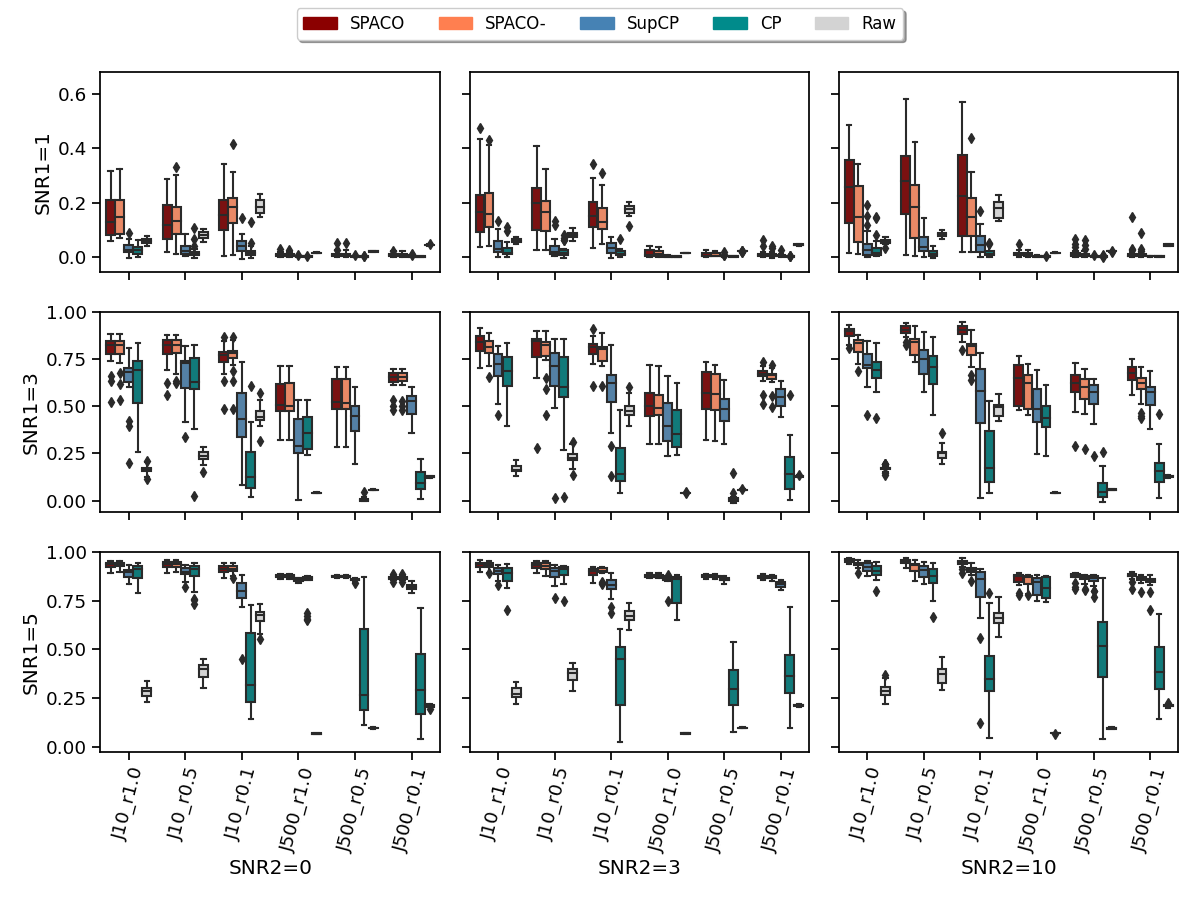
Figure 1: Reconstruction evaluation by the correlations between the estimates and the true signal tensor. In each subplot, x axis label indicates different JJ and observing rate, the y axis is the achieved correlation, and the box colors represent different methods. The corresponding subplot column/row name represents the signal-to-noise ratio SNR1/SNR2.
Refer to caption

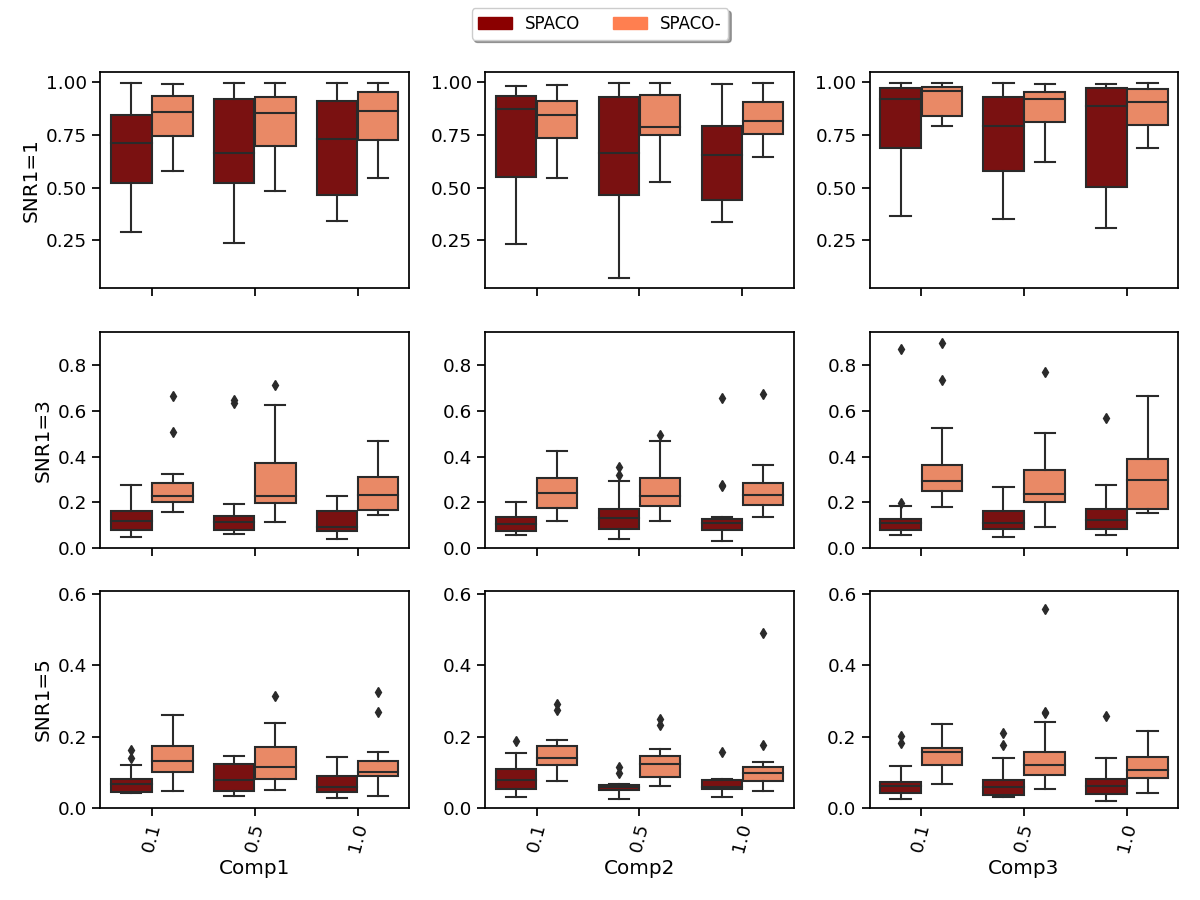
SPACO outperforms SPACO- when the subject score UU depends strongly on ZZ, which could result from a more accurate estimation of the subject scores. To confirm this, we evaluate the estimation quality of UU at J=10J=10 and SNR2=10=10 and measure the estimation quality by R2R^{2} (regressing the true subject scores on the estimated ones). In Figure 2, we shows the achieved (1R2)(1-R^{2}) for SPACO and SPACO- (smaller is better), where x-axis label represents the observing rate and column names represent the component, e.g., Comp1U1\rightarrow U_{1}.

Figure 2: Comparison of SPACO and SPACO- for reconstructing UU at J=10J=10, SNR2=10=10. In each subplot, x axis label indicates different component and observing rate, the y axis is the achieved (1R2)(1-R^{2}), and the box colors represent different methods. The corresponding subplot column/row name represents the signal-to-noise ratio SNR1/component.
Refer to caption

SPACO /SPACO- are both top performers for our smooth tensor decomposition problem and achieve significantly better performance than CP and SupCP when the signal is weak and when the missing rate is high by utilizing the smoothness of the time trajectory. To see this, we compared the estimation quality of the time trajectories using SPACO and SupCP. In Figure 3, we shows the achieved (1R2)(1-R^{2}) for SPACO and SupCP at J=10J=10. In the x-axis label represents different trajectory and observed rate, e.g., (C1r1.0C1_{r}1.0\rightarrow estimation of ϕ1(t)\phi_{1}(t) at observing rate r=1.0r=1.0). When the signal is weak (SNR1=1), SPACO could approximate the constant trajectory component (C1C1) and start to estimate other trajectories successfully as the signal increases. SPACO achieves significantly better estimation of the true underlying trajectories than SupCP for various signal-to-noise ratios.
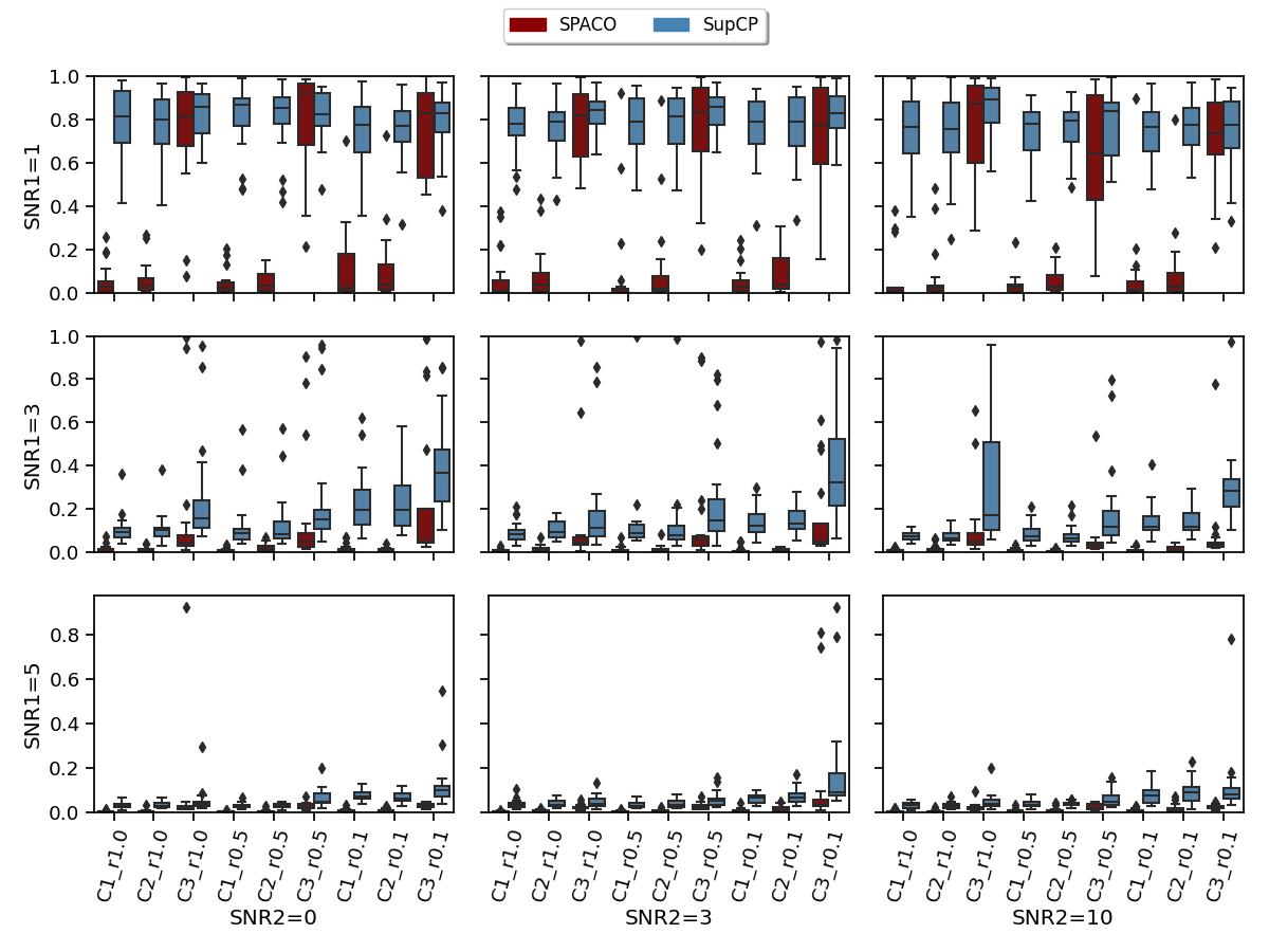
Figure 3: Comparison of SPACO and SupCP for reconstructing Φ\Phi at J=10J=10. In each subplot, x axis label indicates different component and observing rate, the y axis is the achieved (1R2)(1-R^{2}), and the box colors represent different methods. The corresponding subplot column/row name represents the signal-to-noise ratio SNR1/SNR2.
Refer to caption

5.2 Variable importance and hypothesis testing

We investigate the approximated p-values based on cross-fit for testing the partial and marginal associations of 𝒁\bm{Z} with 𝜼{\bm{\eta}} under the same simulation set-ups. Since our variables in 𝒁\bm{Z} are generated independently, the two null hypotheses coincide in this setting. However, the two tests have different powers given the same p-value cut-off because the test statistics differ.

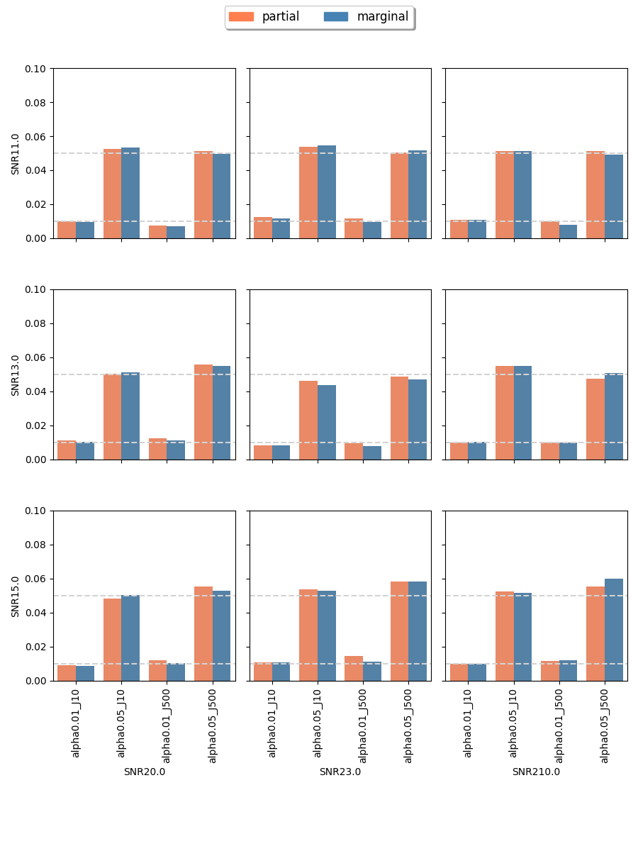
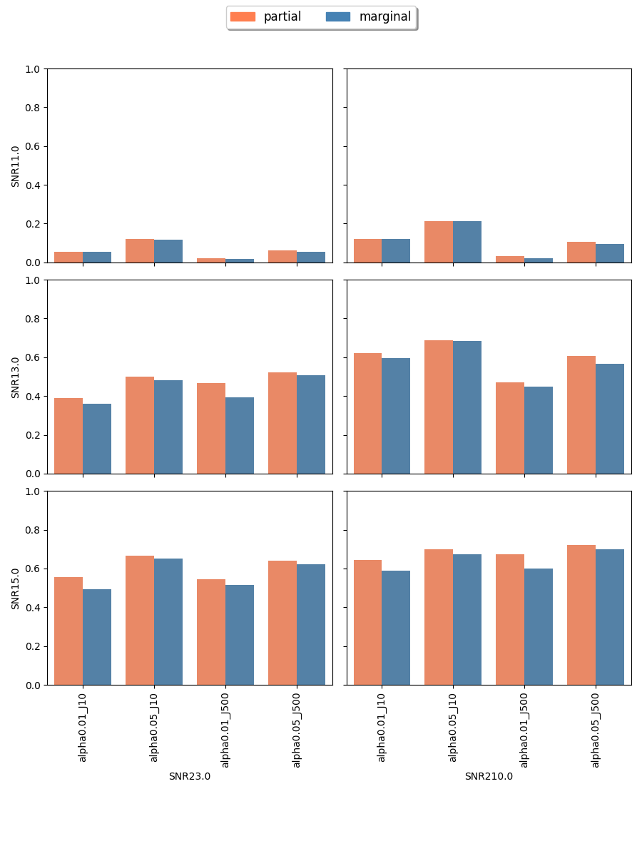
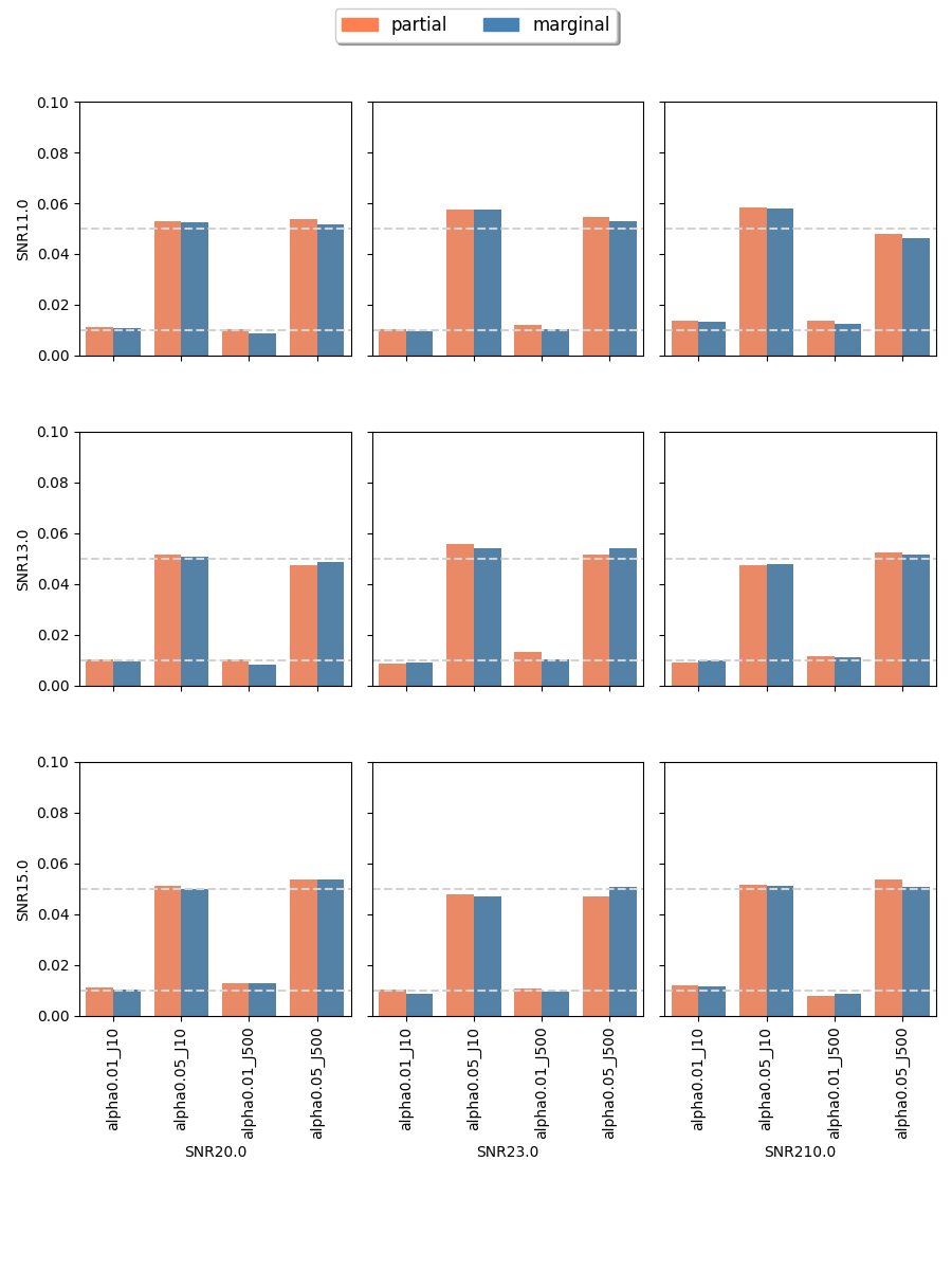
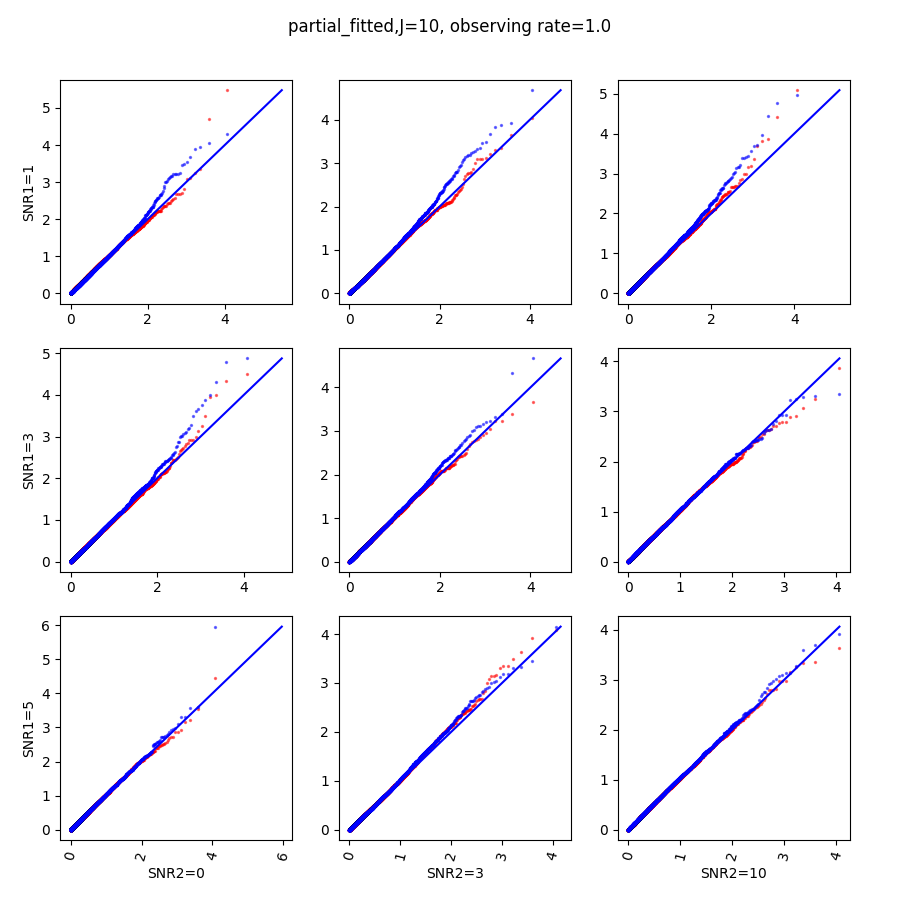
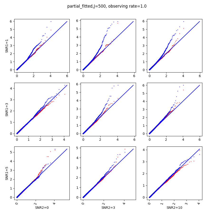
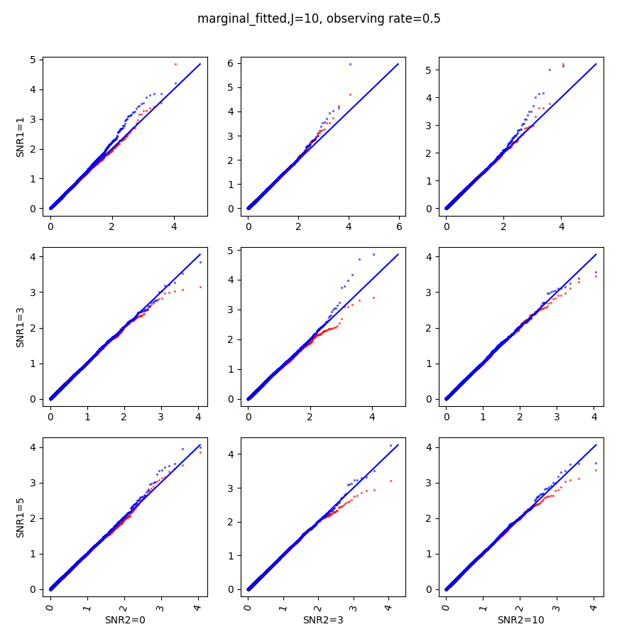
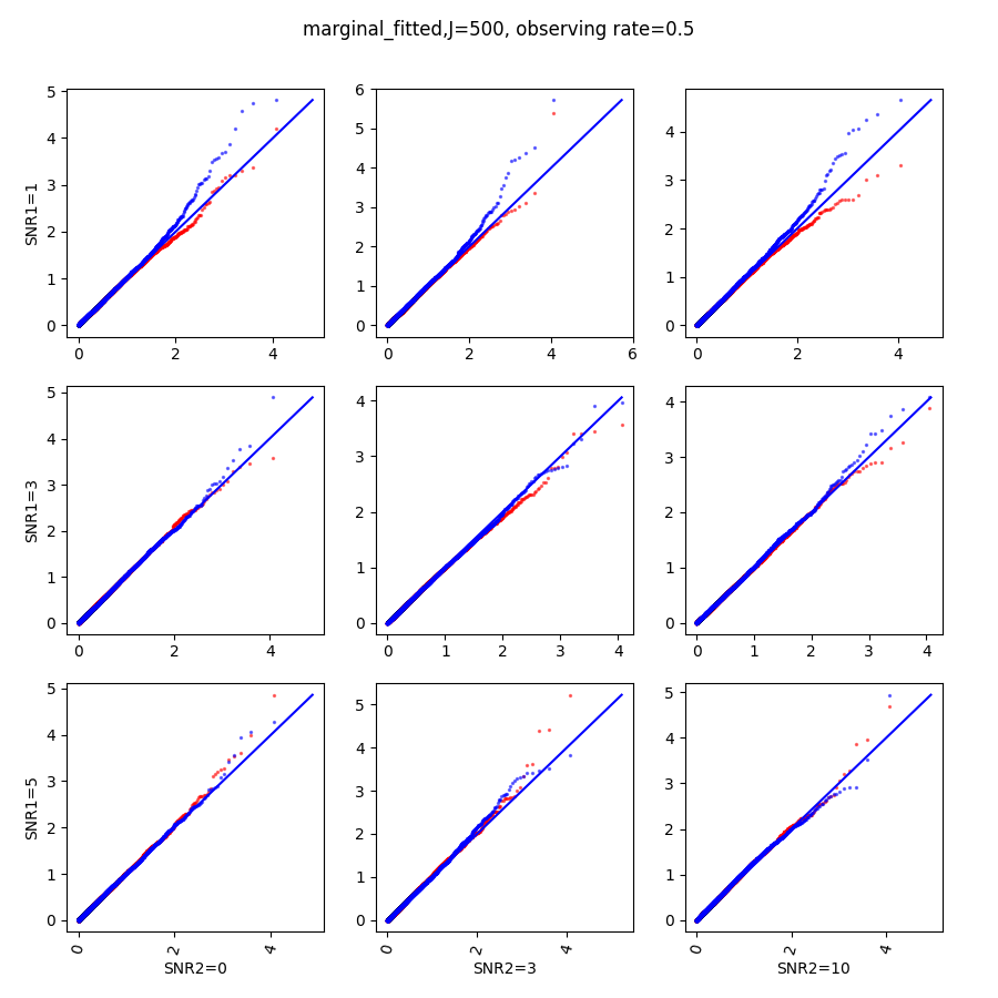
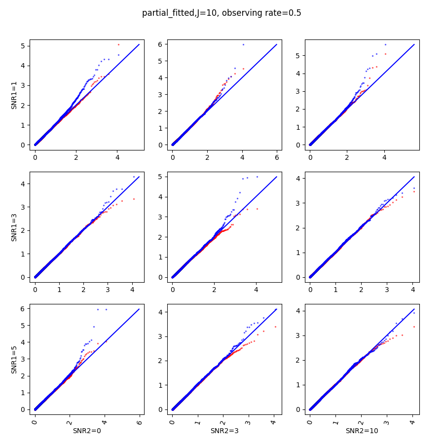
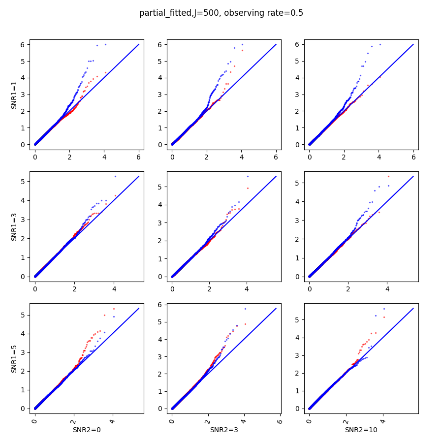
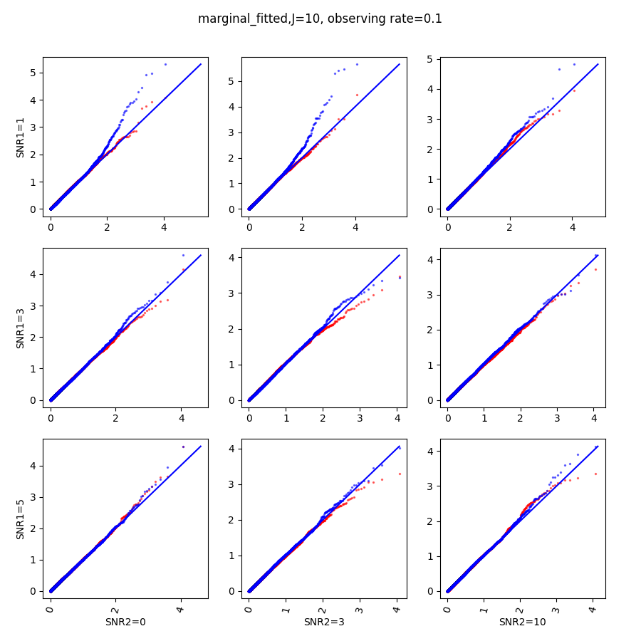
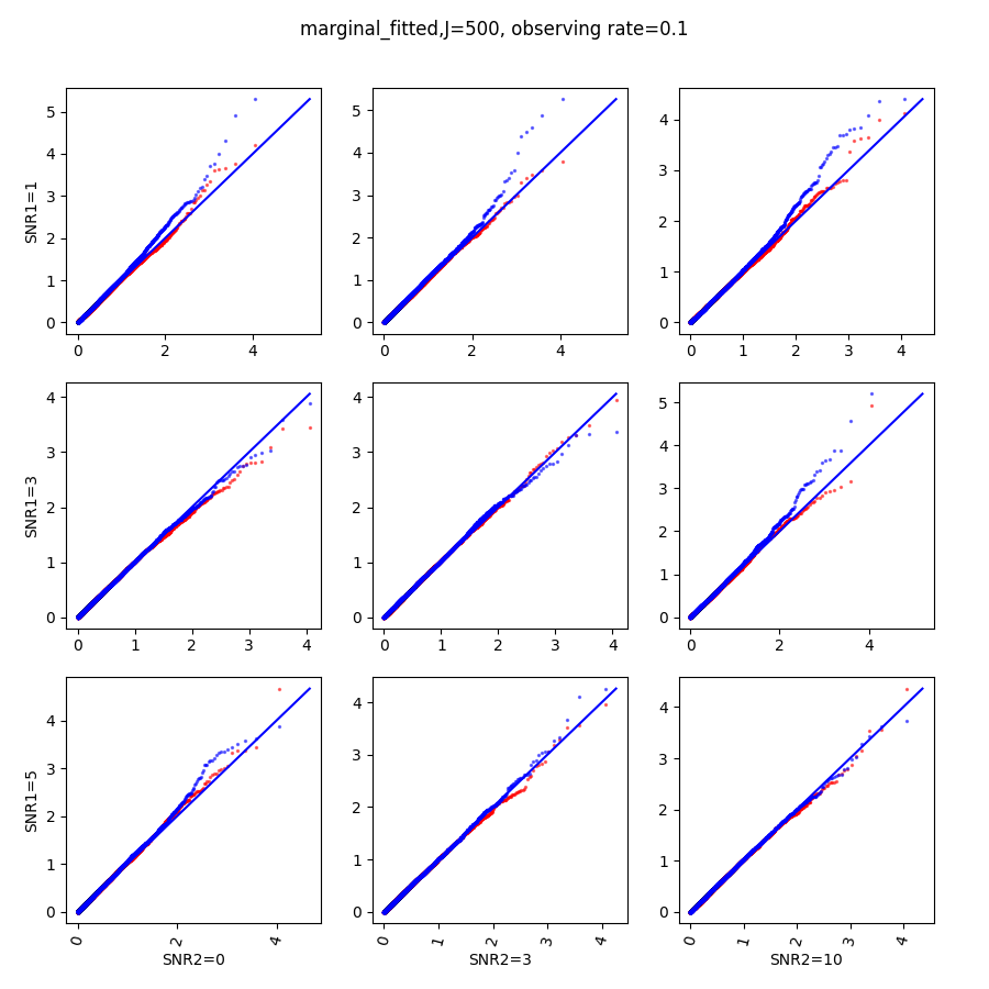
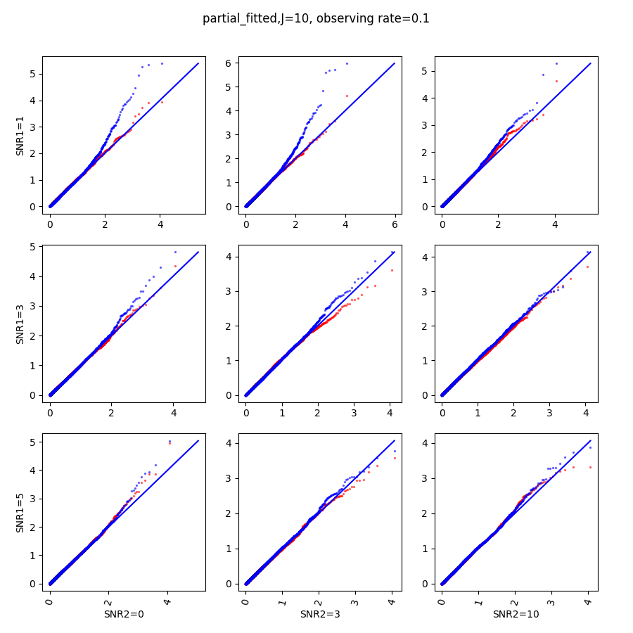
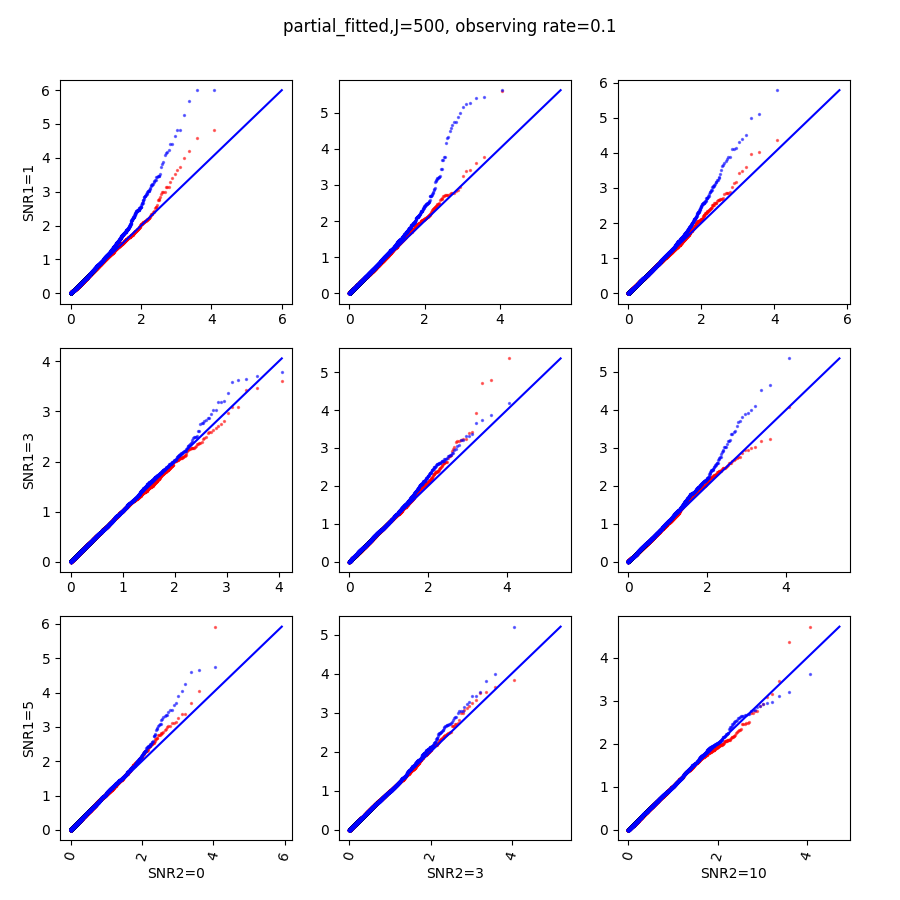
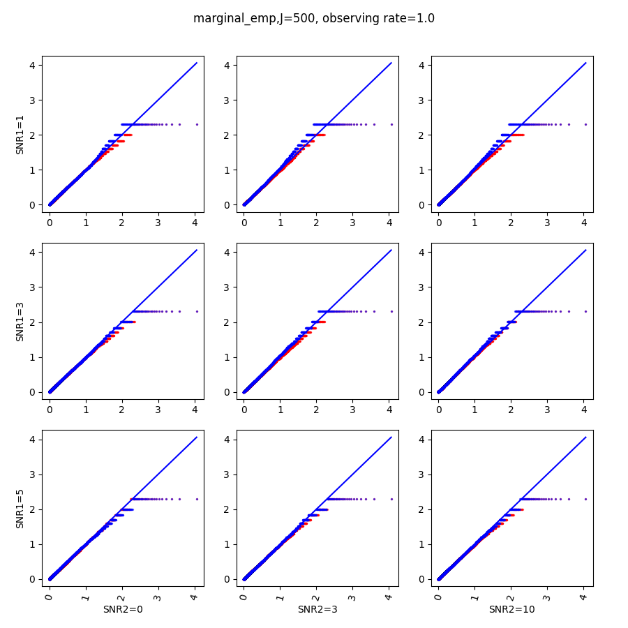
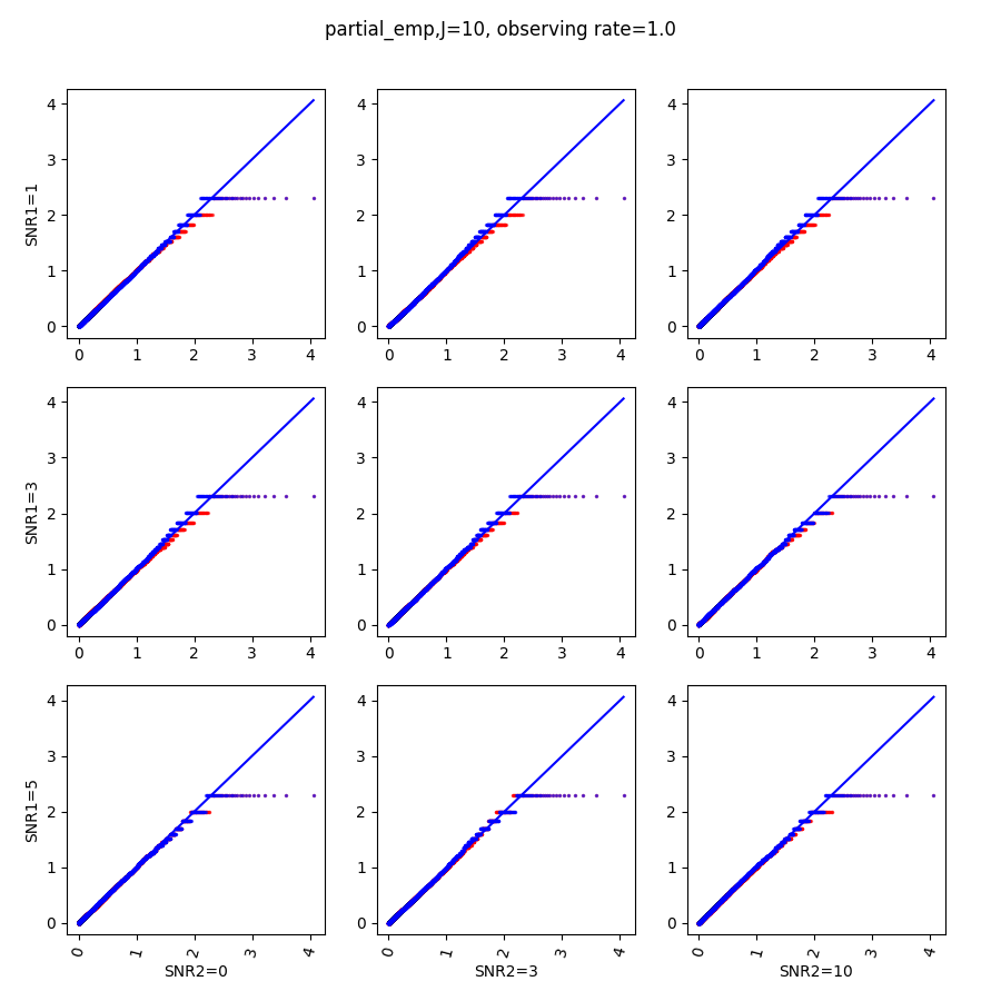
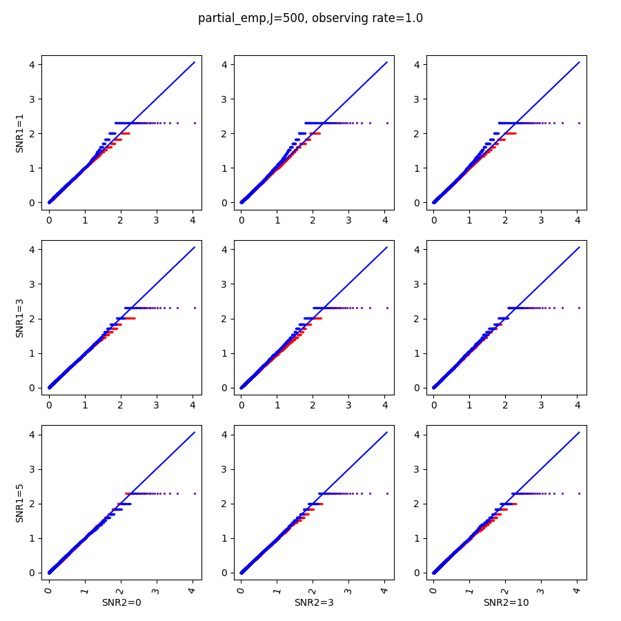
The proposed randomization tests for SPACO achieve reasonable Type I error controls. Cross-fit is important for a good Type I error control: In Appendix C.4, we present qq-plots comparing p-values using cross-fitted 𝑽\bm{V} and 𝚽\bm{\Phi} and the naive construction. We observe noticeable deviations from the uniform distribution for the later construction when the signal-to-noise ratio is low. Fig.10 and Fig.5 show the the achieved Type I error and power with p-value cut-offs at α=0.01,0.05\alpha=0.01,0.05 and with observed rate r=0.5r=0.5. The type I errors are also well controlled for r{1.0,0.1}r\in\{1.0,0.1\} (Appendix C.3).

Figure 4: Achieved type I errors at observing rate r=0.5r=0.5. In each subplot, x axis label indicates different combination of feature dimension JJ and targeted level α{0.01,0.05}\alpha\in\{0.01,0.05\}, the y axis is the achieved type I errors. Different bar colors represent different tests (partial or marginal). The two dashed horizontal lines indicate levels 0.01 and 0.05.
Refer to caption
Figure 5: Achieved power at observing rate r=0.5r=0.5. In each subplot, x axis label indicates different combination of feature dimension JJ and targeted level α{0.01,0.05}\alpha\in\{0.01,0.05\}, the y axis is the achieved power. Different bar colors represent different tests (partial or marginal).
Refer to caption

6 Case study

We now apply SPACO to a longitudinal immunological data set on COVID 19 from the IMPACT study (Lucas et al., 2020). Initially, the data contained 180 samples on 135 immunological features, collected from 98 participants with COVID-19 infection. We filter out features with more than 20%20\% missingness among collected samples and imputed the missing observations using MOFA (Argelaguet et al., 2018) for the remaining features. This leaves us with a complete matrix with 111 features and 180 samples, which is organized into a tensor of size (I,T,J)=(98,35,111)(I,T,J)=(98,35,111) where TT is the number of unique DFSO (days from symptom onsite) in this data set. This is a sparsely observed tensor, and the average observing rate is 1.84 along the time dimension. Apart from the immunological data, the data set also provides non-immunological covariates. We use eight static risk factors as our covariate 𝒁\bm{Z} (COVID_risk1 - COVID_risk5, age, sex, BMI), and four symptom measures as additional responses (ICU, Clinical score, LengthofStay, Coagulopathy).
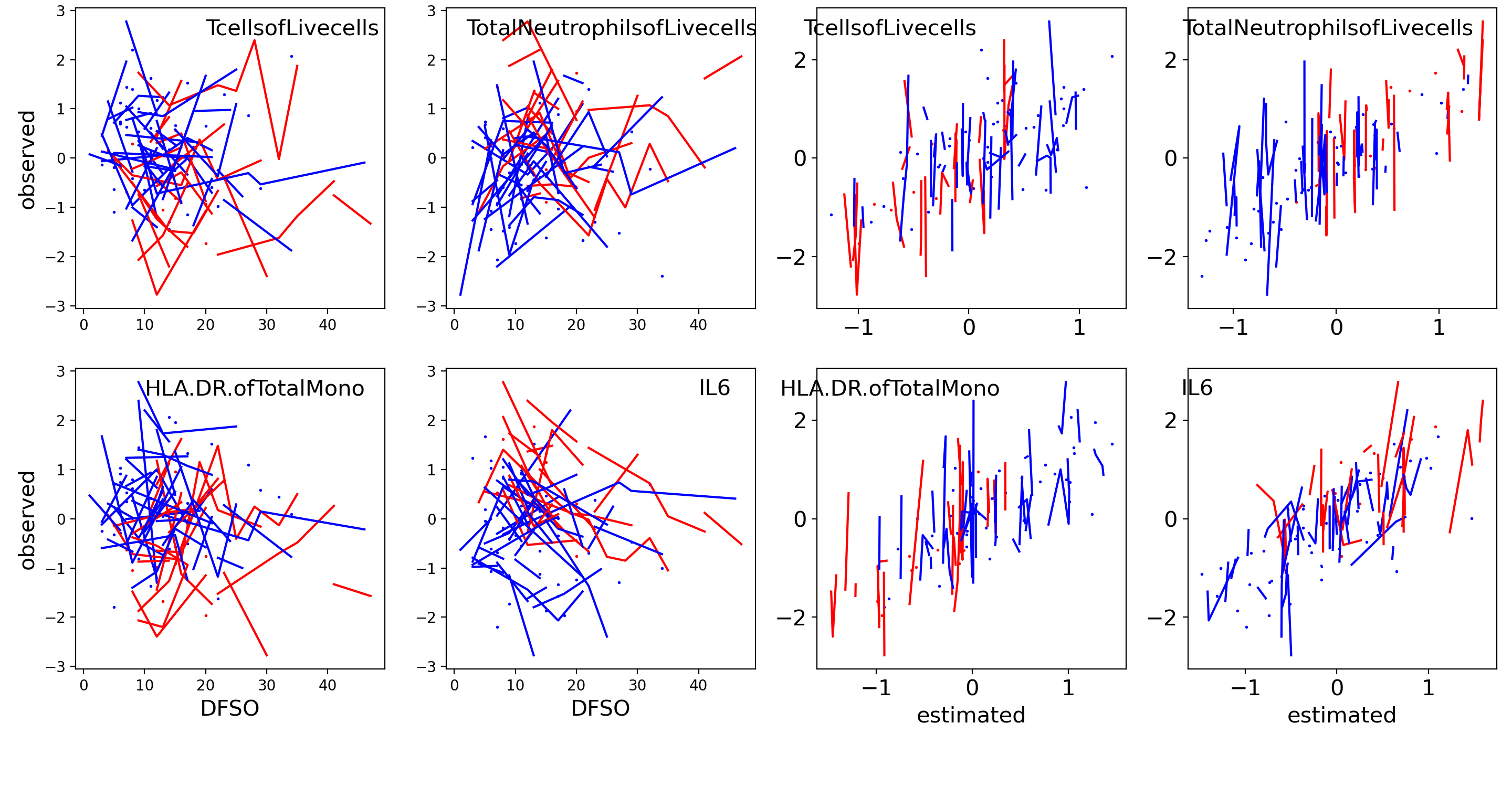
Figure 6: Left panel shows examples of time trajectories of four features for different subjects (horizontal time axis is the DFSO ) ; right panel shows plots of observed feature values against estimated ones from SPACO. Each line/dot represents observations from a single subject. Subjects in ICU are colored red.
Refer to caption

We run SPACO with processed 𝑿\bm{X}, 𝒁\bm{Z}, and model rank K=4K=4, selected from finding the first maxima for the five-fold cross-validated marginal log-likelihood. Fig.6 shows example plots of raw observations against our reconstructions across all samples. We see a positive correlation between these observed and reconstructed values.

Combining static covariates ZZ with the longitudinal measurements can sometimes improve the estimation quality of subject scores compared to SPACO-, as we have illustrated in our synthetic data examples. We can not possibly get the true subject scores in the real data set. However, we could still compare the estimated subject scores are clinically relevant by comparing them to the responses. Here, we also run SPACO- with K=4K=4 and examine if the resulting subject scores from SPACO associate better with the responses. Table 1 shows the spearman correlations and their p-values when comparing the estimated subject scores and each response. The top three components C1, C2, C3 are significantly associated with the responses. Among them, C2C_{2} uniquely captures variability for the length of stay (in hospital), and only C3C3 heavily depends on 𝒁\bm{Z} (the estimated coefficients are 0 for both C1C1 and C2C2). C3 from SPACO achieved a better association with the clinical outcomes than SPACO.

Table 1: Association between estimated subject scores and four response variables. C1-C4 represent the four components in SPACO/SPACO-. C*cor represents the achieved spearman correlation and C*pval is the p-value for the corresponding correlation test.

C1cor C1pval C2cor C2pval C3cor C3pval C4cor C4pval SPACO ICU -0.20 4.9E-02 0.37 1.7E-04 0.28 5.4E-03 0.00 9.8E-01 Clinicalscore -0.32 1.2E-03 0.42 1.3E-05 0.44 6.4E-06 0.07 4.8E-01 LengthofStay -0.10 3.4E-01 0.28 5.2E-03 0.14 1.8E-01 0.11 2.9E-01 Coagulopathy -0.03 7.7E-01 0.22 3.1E-02 0.21 3.5E-02 0.03 7.9E-01 SPACO- ICU -0.20 5.1E-02 0.38 1.4E-04 0.25 1.5E-02 -0.00 9.6E-01 Clinicalscore -0.32 1.3E-03 0.43 1.0E-05 0.40 4.5E-05 0.07 4.9E-01 LengthofStay -0.09 3.9E-01 0.29 4.4E-03 0.10 3.5E-01 0.10 3.3E-01 Coagulopathy -0.03 8.0E-01 0.22 3.0E-02 0.19 5.9E-02 0.02 8.2E-01

Using the randomization test, we can also test for the contribution of each ZjZ_{j} to C3. Table 2 shows the p-value and adjusted p-value from the partial dependence test and marginal dependence test, with the number of randomization B=2000B=2000. The top associate is COVIDRISK_3 (hypertension) with a p-value around 0.01 (adjusted p-value around 0.1). BMI is also weakly associated with C3, with p values <0.05<0.05 for both tests. In this data set, we observe that the immunological measurements contain information strongly related to clinical responses of interest. Although some risk factors like hypertension and BMI contains relatively weaker signal, they may still improve the estimated subject scores like in the case of C3.

Table 2: Results from randomization test for component 3 (C3). The column nonzero counts the number of 1 for binary covariate COVIDRISK_1 - COVIDRISK_5 and sex (1 = Male, 0 = Female). The adjusted pvalues (pval*) are based on BH correction.

pval(partial) pval(marginal) padj(partial) padj(marginal) nonzero COVIDRISK_1 0.877 0.905 1.000 0.905 7 COVIDRISK_2 0.263 0.063 0.701 0.169 24 COVIDRISK_3 0.013 0.011 0.101 0.088 50 COVIDRISK_4 0.563 0.712 1.000 1.000 23 COVIDRISK_5 0.919 0.885 0.919 1.000 5 Age 0.584 0.423 0.935 0.846 sex 0.715 0.727 0.953 0.970 47 BMI 0.029 0.041 0.117 0.166

7 Discussion

We propose SPACO to model sparse multivariate longitudinal data and auxiliary covariates jointly. The smoothness regularization may lead to a dramatic improvement in the estimation quality with high missing rates, and access to informative auxiliary covariates could improve the estimation of subject scores. We applied the proposed pipeline to COVID-19 data sets. Even though both data sets are highly sparse and of small size, SPACO identifies components whose subject scores are strongly associated with clinical outcomes of interest and identify static covariates that might contribute to the severe symptoms. A future direction is to extend SPACO to model multi-omics data. Different omics can be measured at different times and have distinct data types or scales. These motivate a tailored model’s more careful design rather than a naive approach of blindly pooling all omics data together.

SUPPLEMENTARY MATERIAL

Python package for SPACO:

https://github.com/LeyingGuan/SPACO

Python pipeline for reproducing results in the manuscript:

https://github.com/LeyingGuan/SPACOexperments

Appendix A Additional Algorithmic Details

A.1 Updating rules in Algorithm 1

Lemma A.1 provides exact parameter update rules used in Algorithm 1. We also define .\langle.\rangle as the expectation of some quantity with respect to the posterior distribution of 𝑼\bm{U}. Let O{0,1}I×TO\in\{0,1\}^{I\times T} with Oit=1O_{it}=1 if time tt is observed for subject ii and Oit=0O_{it}=0 otherwise.

Lemma A.1

The parameter update steps in Algorithm 1 take the following forms:

  • In line 4, 𝜷k=argmax𝜷k{L(𝑿|Θ)+λ2k|𝜷.k|}=argmin𝜷k12y~𝒁~𝜷k22+λ2k|𝜷k|\bm{\beta}_{k}=\arg\max_{\bm{\beta}_{k}}\{L(\bm{X}|\Theta)+\lambda_{2k}|\bm{\beta}_{.k}|\}=\arg\min_{\bm{\beta}_{k}}\frac{1}{2}\|\tilde{y}-\tilde{\bm{Z}}\bm{\beta}_{k}\|_{2}^{2}+\lambda_{2k}|\bm{\beta}_{k}|, where

    𝐳~i\displaystyle\tilde{\bf z}_{i} =1sk2sk2(Σi)k,ksk2𝐳i,\displaystyle=\sqrt{\frac{1}{s_{k}^{2}}\frac{s_{k}^{2}-(\Sigma_{i})_{k,k}}{s_{k}^{2}}}{\bf z}_{i}, (14)
    y~i\displaystyle\tilde{y}_{i} =1sk2sk2sk2(Σi)k,k((Σi)k,:(𝑽𝚽)iΛi𝑿I,i+lk(Σi)k,l/sl2(𝐳i𝜷l)).\displaystyle=\sqrt{\frac{1}{s_{k}^{2}}\frac{s_{k}^{2}}{s_{k}^{2}-(\Sigma_{i})_{k,k}}}\left((\Sigma_{i})_{k,:}(\bm{V}\odot\bm{\Phi})^{\top}_{\vec{i}}\Lambda_{\vec{i}}\bm{X}_{I,\vec{i}}+\sum_{l\neq k}(\Sigma_{i})_{k,l}/s_{l}^{2}\left({\bf z}_{i}^{\top}\bm{\beta}_{l}\right)\right). (15)

    Here (Σi)k,:(\Sigma_{i})_{k,:} is the kthk^{\text{th}} row of Σi\Sigma_{i}, and (Σi)k,k¯(\Sigma_{i})_{k,\bar{k}} is this row with kthk^{\text{th}} entry removed; Λf,k¯\Lambda_{f,\bar{k}} is the sub matrix of Λf\Lambda_{f} with the kthk^{th} column and row removed.

  • Set Q1=𝑼𝑽IJ×KQ_{1}=\langle\bm{U}\rangle\odot\bm{V}\in{\mathbb{R}}^{IJ\times K}, Q2K×JQ_{2}\in{\mathbb{R}}^{K\times J} and Q3K×K×JQ_{3}\in{\mathbb{R}}^{K\times K\times J} with Q2kj=1σj2𝑿JjjQ1jkQ_{2kj}=\frac{1}{\sigma_{j}^{2}}\bm{X}_{Jj\vec{j}}^{\top}Q_{1\vec{j}k} and Q3k1k2j=1σj2tϕtk1ϕtk2Oit=1(Σik1k2+uik1uik2)Q_{3k_{1}k_{2}j}=\frac{1}{\sigma_{j}^{2}}\sum_{t}\phi_{tk_{1}}\phi_{tk_{2}}\sum_{O_{it}=1}\left(\Sigma_{ik_{1}k_{2}}+\langle u_{ik_{1}}\rangle\langle u_{ik_{2}}\rangle\right). In line 5, the update of 𝑽k\bm{V}_{k} considers the following problem:

    𝑽kargmin𝑽k[j=1J12(ajkvjk22bjkvjk)+ν𝑽k22],\bm{V}_{k}\leftarrow\arg\min_{\bm{V}_{k}}[\sum_{j=1}^{J}\frac{1}{2}\left(a_{jk}v_{jk}^{2}-2b_{jk}v_{jk}\right)+\nu\|\bm{V}_{k}\|_{2}^{2}],

    where ajk=1σj2Q1,j,k22+Q3kk,ja_{jk}=\frac{1}{\sigma_{j}^{2}}\|Q_{1,\vec{j},k}\|_{2}^{2}+Q_{3kk,j}, bjk=Q2kjkkQ3kk,jvjkb_{jk}=Q_{2kj}-\sum_{k^{\prime}\neq k}Q_{3kk^{\prime},j}v_{jk^{\prime}} and ν\nu is the largest value such that the solution satisfies 𝑽k22=1\|\bm{V}_{k}\|_{2}^{2}=1.

  • Set Q1=𝑼𝚽IT×KQ_{1}=\langle\bm{U}\rangle\odot\bm{\Phi}\in{\mathbb{R}}^{IT\times K}, Q2K×TQ_{2}\in{\mathbb{R}}^{K\times T} and Q3K×K×TQ_{3}\in{\mathbb{R}}^{K\times K\times T} with Q2kt=𝑿Tttdiag{1σt2}Q1tkQ_{2kt}=\bm{X}_{Tt\vec{t}}^{\top}\mathrm{diag}\{\frac{1}{\sigma_{\vec{t}}^{2}}\}Q_{1\vec{t}k} and Q3k1k2t=j1σj2vjk1vjk2i:Oit=1(Σik1k2+uik1uik2)Q_{3k_{1}k_{2}t}=\sum_{j}\frac{1}{\sigma_{j}^{2}}v_{jk_{1}}v_{jk_{2}}\sum_{i:O_{it}=1}\left(\Sigma_{ik_{1}k_{2}}+\langle u_{ik_{1}}\rangle\langle u_{ik_{2}}\rangle\right). In line 5, the update of 𝑽k\bm{V}_{k} considers the following problem:

    𝚽kargmin𝚽k[t=1T12(ajkvjk22bjkvjk)+λ1kϕkΩϕk+ν𝚽k22],\bm{\Phi}_{k}\leftarrow\arg\min_{\bm{\Phi}_{k}}[\sum_{t=1}^{T}\frac{1}{2}\left(a_{jk}v_{jk}^{2}-2b_{jk}v_{jk}\right)+\lambda_{1k}\bm{\phi}_{k}^{\top}\Omega\bm{\phi}_{k}+\nu\|\bm{\Phi}_{k}\|_{2}^{2}],

    where atk=(diag{1σt}Q1,t,k22+Q3kk,t)a_{tk}=\left(\|\mathrm{diag}\{\frac{1}{\sigma_{\vec{t}}}\}Q_{1,\vec{t},k}\|_{2}^{2}+Q_{3kk,t}\right), bjk=(Q2ktkkQ3kk,tϕtk)b_{jk}=\left(Q_{2kt}-\sum_{k^{\prime}\neq k}Q_{3kk^{\prime},t}\phi_{tk^{\prime}}\right) and ν\nu is the largest value such that the solution satisfies 𝚽k22=T\|\bm{\Phi}_{k}\|_{2}^{2}=T.

  • In lines 14 and 15,

    sk21Ii[(μik𝐳i𝜷k)2+(Σi)kk],s^{2}_{k}\leftarrow\frac{1}{I}\sum_{i}\left[(\mu_{ik}-{\bf z}_{i}^{\top}\bm{\beta}_{k})^{2}+(\mathbb{\Sigma}_{i})_{kk}\right],

    and

    σj21|j|[(XJ,j(𝚽𝝁)j𝒗j)(XJ,j(𝚽𝝁)j𝒗j)+𝒗j(t(i:Oit=1Σi)(ϕtϕt))𝒗j].\sigma_{j}^{2}\leftarrow\frac{1}{|\vec{j}|}\left[(X_{J,\vec{j}}-(\bm{\Phi}\odot\bm{\mu})_{\vec{j}}\bm{v}_{j})^{\top}(X_{J,\vec{j}}-(\bm{\Phi}\odot\bm{\mu})_{\vec{j}}\bm{v}_{j})+\bm{v}_{j}^{\top}\left(\sum_{t}\left(\sum_{i:O_{it}=1}\mathbb{\Sigma}_{i}\right)\cdot(\bm{\phi}_{t}\bm{\phi}_{t}^{\top})\right)\bm{v}_{j}\right].

Derivation of Lemma A.1 is given in Appendix B.4.

A.2 Functional PCA for initializations

In Yao et al. (2005), the authors suggest a functional PCA analysis by performing eigenvalue decomposition of the smoothed matrix fitted with a local linear surface smoother. Here, we apply the suggested estimation approach on the total product matrix: Let 𝐖^i,s,t=k𝐘is(k)𝐘it(k)\hat{\bf W}_{i,s,t}=\sum_{k}{\bf Y}_{is}(k){\bf Y}_{it}(k) be the empirical estimate of the total product matrix for subject ii, we first estimate 𝔼[W^i,s,t]\mathbb{E}[\hat{W}_{i,s,t}] via local surface smoother and then perform PCA on the estimated 𝔼[W^i,s,t]\mathbb{E}[\hat{W}_{i,s,t}]:

  • To fit a local linear surface smoother for the off-diagonal element of 𝐖s0,t0{\bf W}_{s_{0},t_{0}}, we consider the following problem:

    miniOitOis=1,stκ(ss0hG,tt0hG)(𝐖^i,s,tg((s0,t0),(s,t),β))2,\min\sum_{i}\sum_{O_{it}O_{is}=1,s\neq t}\kappa(\frac{s-s_{0}}{h_{G}},\frac{t-t_{0}}{h_{G}})(\hat{\bf W}_{i,s,t}-g((s_{0},t_{0}),(s,t),\beta))^{2},

    with g((s0,t0),(s,t),β)=β0+β1(ss0)+β2(tt0)g((s_{0},t_{0}),(s,t),\beta)=\beta_{0}+\beta_{1}(s-s_{0})+\beta_{2}(t-t_{0}), and κ:2\kappa:{\mathbb{R}}^{2}\mapsto{\mathbb{R}} is a standard two-dimensional Gaussian kernel.

  • For the diagonal element, we estimate it by local linear regression: for each t0t_{0}:

    miniOit=1κ1(tt0hG)(𝐖^i,t,tg(t0,t,β))2.\min\sum_{i}\sum_{O_{it}=1}\kappa_{1}(\frac{t-t_{0}}{h_{G}})(\hat{\bf W}_{i,t,t}-g(t_{0},t,\beta))^{2}.

    where g(t0,t,β)=β0+β1(tt0)g(t_{0},t,\beta)=\beta_{0}+\beta_{1}(t-t_{0}).

By default, we let hG=T1+st𝟙{iOisOit>0}h_{G}=\frac{T}{\sqrt{1+\sum_{s\neq t}\mathbbm{1}\{\sum_{i}O_{is}O_{it}}>0\}}.

A.3 Parameter tuning on λ1k\lambda_{1k}

In this section, we provide more details on the leave-one-time-out cross-validation for tuning λ1k\lambda_{1k}, k=1,,K\forall\;k=1,\ldots,K. From eq. (19), the expected penalized deviance loss can be written as (keeping only terms relevant to 𝚽\bm{\Phi}):

L\displaystyle L =t=1{ϕt[(𝑽𝝁)t.Λt1(𝑽𝝁)t.+j(Oit=1Σi)(𝒗j𝒗j)σj2]ϕt2ϕt[(𝑽𝝁)t.Λt1]𝑿T,t}\displaystyle=\sum^{\top}_{t=1}\left\{\bm{\phi}_{t}^{\top}\left[(\bm{V}\bigodot\bm{\mu})_{\vec{t}.}^{\top}\Lambda^{-1}_{\vec{t}}(\bm{V}\bigodot\bm{\mu})_{\vec{t}.}+\sum_{j}\frac{\left(\sum_{O_{it}=1}\Sigma_{i}\right)\cdot\left(\bm{v}_{j}\bm{v}_{j}^{\top}\right)}{\sigma_{j}^{2}}\right]\bm{\phi}_{t}-2\bm{\phi}_{t}^{\top}\left[(\bm{V}\bigodot\bm{\mu})_{\vec{t}.}^{\top}\Lambda^{-1}_{\vec{t}}\right]\bm{X}_{T,\vec{t}}\right\}
+kλ1k𝚽kΩ𝚽k.\displaystyle+\sum_{k}\lambda_{1k}\bm{\Phi}_{k}^{\top}\Omega\bm{\Phi}_{k}.

For a given kk, we define the diagonal matrix 𝑨T×T\bm{A}\in{\mathbb{R}}^{T\times T} and the vector aTa\in{\mathbb{R}}^{T} as

𝑨tt\displaystyle\bm{A}_{tt} =[(𝑽𝝁)t.Λt1(𝑽𝝁)t.+j(Oit=1Σi)(𝒗j𝒗j)σj2]kk\displaystyle=\left[(\bm{V}\bigodot\bm{\mu})_{\vec{t}.}^{\top}\Lambda^{-1}_{\vec{t}}(\bm{V}\bigodot\bm{\mu})_{\vec{t}.}+\sum_{j}\frac{\left(\sum_{O_{it}=1}\Sigma_{i}\right)\cdot\left(\bm{v}_{j}\bm{v}_{j}^{\top}\right)}{\sigma_{j}^{2}}\right]_{kk}
at\displaystyle a_{t} =(𝑽k𝝁.k)tΛt1𝑿T,t[(𝑽𝝁)t.Λt1(𝑽𝝁)t.+j(Oit=1Σi)(𝒗j𝒗j)σj2]k,k¯ϕt,k¯.\displaystyle=(\bm{V}_{k}\otimes\bm{\mu}_{.k})^{\top}_{\vec{t}}\Lambda^{-1}_{\vec{t}}\bm{X}_{T,\vec{t}}-\left[(\bm{V}\bigodot\bm{\mu})_{\vec{t}.}^{\top}\Lambda^{-1}_{\vec{t}}(\bm{V}\bigodot\bm{\mu})_{\vec{t}.}+\sum_{j}\frac{\left(\sum_{O_{it}=1}\mathbb{\Sigma}_{i}\right)\cdot\left(\bm{v}_{j}\bm{v}_{j}^{\top}\right)}{\sigma_{j}^{2}}\right]_{k,\bar{k}}^{\top}\bm{\phi}_{t,\bar{k}}.

When we leave out a specific time point t0t_{0}, we optimize for 𝚽k\bm{\Phi}_{k} minimizing the following leave-one-out constrained loss,

min𝚽kJ(t0,k)\displaystyle\min_{\bm{\Phi}_{k}}J(t_{0},k) =𝚽k(𝑨(t0)+λ1kΩ)𝚽k2a(t0)𝚽k,𝚽k22=T.\displaystyle=\bm{\Phi}_{k}^{\top}\left(\bm{A}(t_{0})+\lambda_{1k}\Omega\right)\bm{\Phi}_{k}-2a(t_{0})^{\top}\bm{\Phi}_{k},\quad\|\bm{\Phi}_{k}\|_{2}^{2}=T.

We set 𝑨(t0)\bm{A}(t_{0}) as 𝑨\bm{A} with the (t0,t0)(t_{0},t_{0})-entry zeroed out, and a(t0)a(t_{0}) as aa with a(t0)a(t_{0}) zeroed out. The leave-one-time cross-validation error is calculated based on the expected deviance loss (unpenalized) at the leave-out time point t0t_{0}:

Jloocv(t0,k)\displaystyle J_{loocv}(t_{0},k) =𝑨t0,t0(ϕ^t0kt0at0𝑨t0,t0)2,\displaystyle=\bm{A}_{t_{0},t_{0}}\left(\hat{\phi}^{-t_{0}}_{t_{0}k}-\frac{a_{t_{0}}}{\bm{A}_{t_{0},t_{0}}}\right)^{2},

where ϕ^t0kt0\hat{\phi}^{-t_{0}}_{t_{0}k} is the leave-one-out estimate. To reduce the computational cost, we drop the norm constraint when picking λ1k\lambda_{1k}, which enables us to adopt the following short-cut:

t0Jloocv(t0,k)=t0𝑨t0,t0(ϕ^t0kat0𝑨t0,t0)2(1[(𝑨+λ1kΩ)1]t0t0)2,\sum_{t_{0}}J_{loocv}(t_{0},k)=\sum_{t_{0}}\frac{\bm{A}_{t_{0},t_{0}}\left(\hat{\phi}_{t_{0}k}-\frac{a_{t_{0}}}{\bm{A}_{t_{0},t_{0}}}\right)^{2}}{\left(1-[(\bm{A}+\lambda_{1k}\Omega)^{-1}]_{t_{0}t_{0}}\right)^{2}}, (16)

where 𝚽^k\hat{\bm{\Phi}}_{k} is the unconstrained solution from using all time points. This follows from the arguments below:

  1. 1.

    Drop the constraint, the original problem is equivalent to:

    min(𝑨(t0)+λ1kΩ)12𝚽k(𝑨(t0)+λ1kΩ)12a(t0)22\min\|(\bm{A}(t_{0})+\lambda_{1k}\Omega)^{\frac{1}{2}}\bm{\Phi}_{k}-(\bm{A}(t_{0})+\lambda_{1k}\Omega)^{-\frac{1}{2}}a(t_{0})\|_{2}^{2}
  2. 2.

    Consider the augmented problem:

    min(𝑨+λ1kΩ)12𝚽k(𝑨+λ1kΩ)12a~(t0)22\min\|(\bm{A}+\lambda_{1k}\Omega)^{\frac{1}{2}}\bm{\Phi}_{k}-(\bm{A}+\lambda_{1k}\Omega)^{-\frac{1}{2}}\tilde{a}(t_{0})\|_{2}^{2}

    where a~(t0)=a(t0)+δ(t0)\tilde{a}(t_{0})=a(t_{0})+\delta(t_{0}), and δt0(t0)=At0,t0ϕ^t0kt0\delta_{t_{0}}(t_{0})=A_{t0,t_{0}}\hat{\phi}_{t_{0}k}^{-t_{0}} and δt(t0)=0\delta_{t}(t_{0})=0 for tt0t\neq t_{0}. The augmented problem also has 𝚽^kt0\hat{\bm{\Phi}}^{-t_{0}}_{k} as its solution.

  3. 3.

    Hence, without the constraint, we have 𝚽^k=(𝑨+λ1kΩ)1a\hat{\bm{\Phi}}_{k}=(\bm{A}+\lambda_{1k}\Omega)^{-1}a and 𝚽^kt0=(𝑨+λ1kΩ)1a~(t0)\hat{\bm{\Phi}}_{k}^{-t_{0}}=(\bm{A}+\lambda_{1k}\Omega)^{-1}\tilde{a}(t_{0}). Consequently:

    ϕ^t0kϕ^t0kt0=[(𝑨+λ1kΩ)1]t0t0(at0a~t0(t0))=[(𝑨+λ1kΩ)1]t0t0(at0𝑨t0t0ϕ^t0kt0).\hat{\phi}_{t_{0}k}-\hat{\phi}^{-t_{0}}_{t_{0}k}=[(\bm{A}+\lambda_{1k}\Omega)^{-1}]_{t_{0}t_{0}}(a_{t_{0}}-\tilde{a}_{t_{0}}(t_{0}))=[(\bm{A}+\lambda_{1k}\Omega)^{-1}]_{t_{0}t_{0}}(a_{t_{0}}-\bm{A}_{t_{0}t_{0}}\hat{\phi}_{t_{0}k}^{-t_{0}}).
  4. 4.

    Finally, we obtain

    ϕ^t0kat0𝑨t0t0=ϕ^t0kt0at0At0t0+[(𝑨+λ1kΩ)1]t0t0(at0𝑨t0t0ϕ^t0kt0)\displaystyle\hat{\phi}_{t_{0}k}-\frac{a_{t_{0}}}{\bm{A}_{t_{0}t_{0}}}=\hat{\phi}_{t_{0}k}^{-t_{0}}-\frac{a_{t_{0}}}{A_{t_{0}t_{0}}}+[(\bm{A}+\lambda_{1k}\Omega)^{-1}]_{t_{0}t_{0}}(a_{t_{0}}-\bm{A}_{t_{0}t_{0}}\hat{\phi}_{t_{0}k}^{-t_{0}})
    \displaystyle\Rightarrow ϕ^t0kat0𝑨t0t0=(1𝑨t0t0[(𝑨+λ1kΩ)1]t0t0)(ϕ^t0kt0at0𝑨t0t0)\displaystyle\hat{\phi}_{t_{0}k}-\frac{a_{t_{0}}}{\bm{A}_{t_{0}t_{0}}}=(1-\frac{\bm{A}_{t_{0}t_{0}}}{[(\bm{A}+\lambda_{1k}\Omega)^{-1}]_{t_{0}t_{0}}})(\hat{\phi}_{t_{0}k}^{-t_{0}}-\frac{a_{t_{0}}}{\bm{A}_{t_{0}t_{0}}})

    Hence, we have𝑨t0,t0(ϕ^t0kat0𝑨t0,t0)2(1[(𝑨+λ1kΩ)1]t0t0)2=𝑨t0,t0(ϕ^t0kt0at0𝑨t0,t0)2.\frac{\bm{A}_{t_{0},t_{0}}\left(\hat{\phi}_{t_{0}k}-\frac{a_{t_{0}}}{\bm{A}_{t_{0},t_{0}}}\right)^{2}}{\left(1-[(\bm{A}+\lambda_{1k}\Omega)^{-1}]_{t_{0}t_{0}}\right)^{2}}=\bm{A}_{t_{0},t_{0}}\left(\hat{\phi}^{-t_{0}}_{t_{0}k}-\frac{a_{t_{0}}}{\bm{A}_{t_{0},t_{0}}}\right)^{2}.

A.4 Generation of randomized covariates for testing

In the simulations and real data examples, we encounter two types of ZjZ_{j}: Gaussian and binary. We model the conditional distribution of ZjZ_{j} given ZjcZ_{j^{c}} with a (penalized) GLM. For Gaussian data, we consider a model where

Zj=Zjcθ+ϵj,ϵj𝒩(0,σ2).Z_{j}=Z_{j^{c}}\theta+\epsilon_{j},\quad\epsilon_{j}\sim\mathcal{N}(0,\sigma^{2}).

We estimate θ\theta and σ2\sigma^{2} empirically from data. When qq, the dimension of ZZ, is large, we apply a lasso penalty on β\beta with penalty level selected with cross-validation. Let θ^\hat{\theta} and σ^2\hat{\sigma}^{2} be our estimates of the distribution parameters. We then generate new 𝐳i{\bf z}_{i}^{*} for subject ii from the estimated distribution 𝐳i=𝐳i,jcθ^+ϵij{\bf z}_{i}^{*}={\bf z}_{i,j^{c}}^{\top}\hat{\theta}+\epsilon_{ij}^{*}, with ϵij\epsilon_{ij}^{*} independently generated from 𝒩(0,σ^2)\mathcal{N}(0,\hat{\sigma}^{2}). For binary ZjZ_{j}, we consider the model

logP(Zj=1)1P(Zj=1)=Zjcθ.\log\frac{P(Z_{j}=1)}{1-P(Z_{j}=1)}=Z_{j^{c}}\theta.

Again, we estimate θ\theta empirically, with cross-validated lasso penalty for large qq. We then generate zijz_{ij}^{*} independently from

P(Zj=1|𝐳jc)=11+exp(𝐳i,jcθ^).P(Z_{j}=1|{\bf z}_{j^{c}})=\frac{1}{1+\exp(-{\bf z}_{i,j^{c}}^{\top}\hat{\theta})}.

To generate ZjZ_{j}^{*} from the marginal distribution of ZjZ_{j}, instead of estimating this distribution, we let 𝒁j\bm{Z}_{j}^{*} be a random permutation of 𝒁j\bm{Z}_{j}.

The randomization test requires generating ZjZ_{j}^{*} from the conditional or marginal distribution of ZjZ_{j}, and estimating the resulting distribution of TT^{*}. We will estimate the distribution of TT^{*} by fitting a skewed t-distribution as suggested in (Katsevich and Roeder, 2020). The use of the fitted G^(.)\hat{G}(.) instead of the naive empirical CDF can greatly reduce the computational cost: We may obtain accurate estimates of small p-values around 10410^{-4} using only 200 independent generations of ZjZ_{j}^{*} and the fitted G^(.)\hat{G}(.).

Appendix B Proofs

B.1 Proof of Theorem 3.1

The first step leads to non-decreasing marginal log-likelihood by definition, while the second step is a EM procedure. If we can show that the penalized marginal log-likelihood is non-decreasing at each subroutine of the EM procedure, we prove Theorem 3.1.

For simplicity, θ\theta be the parameters that is being updated in some subroutine and Θθ\Theta_{\setminus\theta} parameters excluding θ\theta. Let Θ=Θθθ\Theta=\Theta_{\setminus\theta}\cup\theta, Θ=Θθ\Theta^{\prime}=\Theta_{\setminus}\cup\theta. It is known that if a new θ\theta^{\prime} is no worse compared with θ\theta using the EM objective, it is no worse than θ\theta when it comes to the (regularized) marginal MLE (Dempster et al., 1977). We include the short proof here for completeness.

Because the log of the posterior of 𝑼\bm{U} can be decomposed into the difference between the log of the log complete likelihood and the log marginal likelihood, L(𝑼|𝑿,Θ)=L(𝑼,𝑿|Θ)L(𝑿|Θ)L(\bm{U}|\bm{X},\Theta)=L(\bm{U},\bm{X}|\Theta)-L(\bm{X}|\Theta), we have (expectation with respect to posterior distribution of 𝑼\bm{U} with parameters Θ\Theta):

𝔼ΘL(𝑼,𝑿|Θ)=𝔼ΘL(𝑿|Θ)+𝔼ΘL(𝑼|𝑿,Θ)=L(𝑿|Θ)+𝔼ΘL(𝑼|𝑿,Θ).\displaystyle\mathbb{E}_{\Theta}L(\bm{U},\bm{X}|\Theta^{\prime})=\mathbb{E}_{\Theta}L(\bm{X}|\Theta^{\prime})+\mathbb{E}_{\Theta}L(\bm{U}|\bm{X},\Theta^{\prime})=L(\bm{X}|\Theta^{\prime})+\mathbb{E}_{\Theta}L(\bm{U}|\bm{X},\Theta^{\prime}).

As a result, when

𝔼ΘL(X,𝑼|Θ)𝔼ΘL(X,𝑼|Θ),\mathbb{E}_{\Theta}L(X,\bm{U}|\Theta^{\prime})\geq\mathbb{E}_{\Theta}L(X,\bm{U}|\Theta),

the following inequality holds,

L(𝑿|Θ)L(𝑿|Θ)\displaystyle L(\bm{X}|\Theta^{\prime})-L(\bm{X}|\Theta) ={𝔼ΘL(𝑿|Θ)+𝔼ΘL(𝑼|𝑿,Θ)L(𝑿|Θ)}+{𝔼ΘL(𝑼|𝑿,Θ)𝔼ΘL(𝑼|𝑿,Θ)}\displaystyle=\{\mathbb{E}_{\Theta}L(\bm{X}|\Theta^{\prime})+\mathbb{E}_{\Theta}L(\bm{U}|\bm{X},\Theta^{\prime})-L(\bm{X}|\Theta^{\prime})\}+\{\mathbb{E}_{\Theta}L(\bm{U}|\bm{X},\Theta^{\prime})-\mathbb{E}_{\Theta}L(\bm{U}|\bm{X},\Theta)\}
𝔼ΘlogP(𝑼|𝑿,Θ)P(𝑼|𝑿,Θ)0.\displaystyle\geq\mathbb{E}_{\Theta}\log\frac{P(\bm{U}|\bm{X},\Theta)}{P(\bm{U}|\bm{X},\Theta^{\prime})}\geq 0.

The last inequality is due to the fact that the mutual information 𝔼ΘlogP(𝑼|𝑿,Θ)P(𝑼|𝑿,Θ)\mathbb{E}_{\Theta}\log\frac{P(\bm{U}|\bm{X},\Theta)}{P(\bm{U}|\bm{X},\Theta^{\prime})} is nonnegative. Now, we return to our subroutines for updating parameters (𝑽,𝚽,s2,σ2)(\bm{V},\bm{\Phi},s^{2},\sigma^{2}):

  • For our subroutines of updating s2s^{2} and σ2\sigma^{2}, they are defined as the maximizers of 𝔼ΘL(X,𝑼|Θθ,θ)\mathbb{E}_{\Theta}L(X,\bm{U}|\Theta_{-\theta},\theta).

  • From the proof to Lemma A.1 in deriving the explicit form for updating 𝚽\bm{\Phi} and 𝑽\bm{V} (see section), we know that J(𝑽k)J(\bm{V}_{k}) is a convex quadratic loss and J(𝑽k)=j=1J(ajkvjk2+bjkvjk)J(\bm{V}_{k})=\sum_{j=1}^{J}\left(a_{jk}v_{jk}^{2}+b_{jk}v_{jk}\right) for coefficients with explicit forms. If we can show that

    𝑽kminVkJ(𝑽k)+ν𝑽k22𝑽k22=1,\bm{V}_{k}\leftarrow\min_{V_{k}}J(\bm{V}_{k})+\nu\|\bm{V}_{k}\|_{2}^{2}\quad\|\bm{V}_{k}\|_{2}^{2}=1,

    is an minimizer to the problem {minVkJ(𝑽k),s.t.𝑽k22=1}\{\min_{V_{k}}J(\bm{V}_{k}),\;s.t.\|\bm{V}_{k}\|_{2}^{2}=1\}, then updating 𝑽k\bm{V}_{k} to this new vector is valid and will not increase our loss. This is true by standard optimization arguments. Let L(𝑽k,ν)=min𝑽kmaxν[J(𝑽k)+ν(𝑽k221)]L(\bm{V}_{k},\nu)=\min_{\bm{V}_{k}}\max_{\nu}\left[J(\bm{V}_{k})+\nu(\|\bm{V}_{k}\|_{2}^{2}-1)\right]. Let ν\nu be such a value such that 𝑽k22=1\|\bm{V}_{k}\|_{2}^{2}=1, and let 𝑽k\bm{V}_{k}^{*} be the solution at this ν\nu. Then,

    J(𝑽k)=min𝑽kL(𝑽k,ν)min𝑽kmaxνL(𝑽k,ν)=min𝑽k22J(𝑽k)J(𝑽k).J(\bm{V}_{k}^{*})=\min_{\bm{V}_{k}}L(\bm{V}_{k},\nu)\leq\min_{\bm{V}_{k}}\max_{\nu}L(\bm{V}_{k},\nu)=\min_{\|\bm{V}_{k}\|_{2}^{2}}J(\bm{V}_{k})\leq J(\bm{V}_{k}^{*}).

    Hence, the proposed strategy at line 5 in Algorithm 1 solves the original problem. The same arguments hold for updating 𝚽k\bm{\Phi}_{k}.

Hence, given Θ\Theta^{\ell} the posterior distribution at the beginning of iteration \ell, if we update the model parameters at proposed to acquire Θ+1\Theta^{\ell+1}, we always have J(Θ+1)J(Θ)J(\Theta^{\ell+1})\leq J(\Theta^{\ell}).

B.2 Proof of Lemma 4.1

Statement I: Suppose 𝑿I=𝑼𝑴U\bm{X}_{I}=\bm{U}_{\perp}\bm{M}^{\top}_{U}, 𝑿T=𝚽𝑴T\bm{X}_{T}=\bm{\Phi}_{\perp}\bm{M}^{\top}_{T} and 𝑿T=𝑽𝑴V\bm{X}_{T}=\bm{V}^{\top}_{\perp}\bm{M}_{V} for some matrices 𝑴U\bm{M}_{U}, 𝑴T\bm{M}_{T}, 𝑴V\bm{M}_{V}. Then, there exists a rank-K core-array 𝑮=k=1K𝑨k𝑩k𝑪k\bm{G}=\sum_{k=1}^{K}\bm{A}_{k}\circledcirc\bm{B}_{k}\circledcirc\bm{C}_{k}, such that 𝑼=𝑼𝑨\bm{U}=\bm{U}_{\perp}\bm{A}, 𝚽=𝚽𝑩\bm{\Phi}=\bm{\Phi}_{\perp}\bm{B} and 𝑽=𝑽𝑪\bm{V}=\bm{V}_{\perp}\bm{C} form a PARAFAC decomposition of 𝑿\bm{X}: 𝑿=k=1K𝑼k𝚽k𝑽k.\bm{X}=\sum_{k=1}^{K}\bm{U}_{k}\circledcirc\bm{\Phi}_{k}\circledcirc\bm{V}_{k}. Argument I: Statement I can be checked easily: since 𝑼\bm{U}_{\perp} spans the row space of 𝑿I\bm{X}_{I}, we can find a matrix 𝑨\bm{A} such that if we replace 𝑼\bm{U}^{*} with 𝑼𝑨\bm{U}_{\perp}\bm{A}, we still have a PARAFAC decomposition of 𝑿\bm{X}. We can apply the same arguments to 𝚽,𝑽\bm{\Phi}_{\perp},\bm{V}_{\perp}, and hence prove the statement at the beginning. As a result, we need to show that 𝑼\bm{U}_{\perp}, 𝚽\bm{\Phi}_{\perp} and 𝑽\bm{V}_{\perp} spans the column spaces of the three unfolding matrices and 𝑮~\tilde{\bm{G}} is the unfolding of such a core array along the subject dimension.

  • The proposed 𝑽\bm{V}_{\perp} satisfies the requirement by construction. Hence, we need only to check that 𝑼\bm{U}_{\perp} and 𝚽\bm{\Phi}_{\perp} spans the row space of 𝑿I\bm{X}_{I} and 𝑿T\bm{X}_{T} respectively.

  • The projection of 𝑿J\bm{X}_{J} onto 𝑽\bm{V}_{\perp} results in H=𝑽𝑿j=𝑪(𝚽𝑼)H=\bm{V}_{\perp}^{\top}\bm{X}_{j}=\bm{C}(\bm{\Phi}^{*}\odot\bm{U}^{*})^{\top}, where 𝑪=𝑽𝑽\bm{C}=\bm{V}_{\perp}^{\top}\bm{V}^{*}. Hence, we have

    𝐖=k=1K1I𝐘(k)𝐘(k)=𝚽(k=1K(𝑼𝑪k,.)(𝑼𝑪k,.))𝚽,T=𝚽𝑴𝚽{\bf W}=\sum_{k=1}^{K}\frac{1}{I}{\bf Y}(k)^{\top}{\bf Y}(k)=\bm{\Phi}^{*}\left(\sum_{k=1}^{K}\left(\bm{U}^{*}\cdot\bm{C}_{k,.}\right)^{\top}\left(\bm{U}^{*}\cdot\bm{C}_{k,.}\right)\right)\bm{\Phi}^{*,T}=\bm{\Phi}^{*}\bm{M}\bm{\Phi}^{*\top}

    where 𝑴=K×K\bm{M}={\mathbb{R}}^{K\times K} with 𝑴k=𝑪,𝑪k𝑼,𝑼k\bm{M}_{\ell k}=\langle\bm{C}_{\ell},\bm{C}_{k}\rangle\langle\bm{U}^{*}_{\ell},\bm{U}^{*}_{k}\rangle. Notice that

    𝑿T𝑿T\displaystyle\bm{X}_{T}\bm{X}_{T}^{\top} =𝚽(𝑽𝑼)(𝑽𝑼)𝚽,T\displaystyle=\bm{\Phi}^{*}\left(\bm{V}^{*}\odot\bm{U}^{*}\right)^{\top}\left(\bm{V}^{*}\odot\bm{U}^{*}\right)\bm{\Phi}^{*,T}
    =𝚽((𝑽𝑪1)𝑼1,,(𝑽𝑪K)𝑼K)((𝑽𝑪1)𝑼1,,(𝑽𝑪K)𝑼K)𝚽\displaystyle=\bm{\Phi}^{*}\left((\bm{V}_{\perp}\bm{C}_{1})\otimes\bm{U}^{*}_{1},\ldots,(\bm{V}_{\perp}\bm{C}_{K})\otimes\bm{U}^{*}_{K}\right)^{\top}\left((\bm{V}_{\perp}\bm{C}_{1})\otimes\bm{U}^{*}_{1},\ldots,(\bm{V}_{\perp}\bm{C}_{K})\otimes\bm{U}^{*}_{K}\right)\bm{\Phi}^{*\top}
    =𝚽((𝑪𝑽𝑽𝑪k)(𝑼𝑼k))k𝚽\displaystyle=\bm{\Phi}^{*}\left(\left(\bm{C}^{\top}_{\ell}\bm{V}^{\top}_{\perp}\bm{V}_{\perp}\bm{C}_{k}\right)\otimes(\bm{U}_{\ell}^{\top}\bm{U}_{k})\right)_{\ell k}\bm{\Phi}^{*\top}
    =𝚽((𝑪𝑪k)(𝑼𝑼k))k𝚽=𝚽𝑴𝚽\displaystyle=\bm{\Phi}^{*}\left(\left(\bm{C}^{\top}_{\ell}\bm{C}_{k}\right)(\bm{U}_{\ell}^{\top}\bm{U}_{k})\right)_{\ell k}\bm{\Phi}^{*\top}=\bm{\Phi}^{*}\bm{M}\bm{\Phi}^{*\top}

    Hence, Φ\Phi_{\perp} is the top KK left singular vectors of 𝑿T\bm{X}_{T}. We set 𝑩=𝚽𝚽\bm{B}=\bm{\Phi}_{\perp}^{\top}\bm{\Phi}^{*}.

  • 𝑼~\tilde{\bm{U}} is estimated by regression 𝑿I\bm{X}_{I} on 𝑽𝚽\bm{V}_{\perp}\otimes\bm{\Phi}. Because both 𝑽\bm{V}_{\perp} and 𝚽\bm{\Phi}_{\perp} are orthonormal, 𝑽𝚽\bm{V}_{\perp}\otimes\bm{\Phi}_{\perp} is also orthonormal:

    (𝑽𝚽)(𝑽𝚽)=(𝑽𝑽)(𝚽𝚽)=𝐈dK×K𝐈dK×K=𝐈dK2×K2.(\bm{V}_{\perp}\otimes\bm{\Phi})^{\top}(\bm{V}_{\perp}\otimes\bm{\Phi})=(\bm{V}_{\perp}^{\top}\bm{V}_{\perp})\otimes(\bm{\Phi}^{\top}\bm{\Phi}_{\perp})={\rm{\mathbf{I}d}}_{K\times K}\otimes{\rm{\mathbf{I}d}}_{K\times K}={\rm{\mathbf{I}d}}_{K^{2}\times K^{2}}.

    Hence, we have

    𝑼~(𝑽𝚽)\displaystyle\tilde{\bm{U}}(\bm{V}_{\perp}\otimes\bm{\Phi}_{\perp})^{\top} =11+δ𝑿I(𝑽𝚽)(𝑽𝚽)\displaystyle=\frac{1}{1+\delta}\bm{X}_{I}(\bm{V}_{\perp}\otimes\bm{\Phi}_{\perp})(\bm{V}_{\perp}\otimes\bm{\Phi}_{\perp})^{\top}
    =11+δ𝑿I((𝑽𝑽)(𝚽𝚽))\displaystyle=\frac{1}{1+\delta}\bm{X}_{I}((\bm{V}_{\perp}\bm{V}_{\perp}^{\top})\otimes(\bm{\Phi}_{\perp}\bm{\Phi}_{\perp}^{\top}))
    =11+δ𝑼((𝑽𝑪)(𝚽𝑩))(𝑽𝚽)(𝑽𝚽)\displaystyle=\frac{1}{1+\delta}\bm{U}^{*}\left((\bm{V}_{\perp}\bm{C})\odot(\bm{\Phi}_{\perp}\bm{B})\right)^{\top}(\bm{V}_{\perp}\otimes\bm{\Phi}_{\perp})(\bm{V}_{\perp}\otimes\bm{\Phi}_{\perp})^{\top}
    =𝑼((𝑪1𝑽𝑽𝑽)(𝑩1𝚽𝚽𝚽)(𝑪K𝑽𝑽𝑽)(𝑩K𝚽𝚽𝚽))(𝑽𝚽)\displaystyle=\bm{U}^{*}\left(\begin{array}[]{c}(\bm{C}^{\top}_{1}\bm{V}^{\top}_{\perp}\bm{V}_{\perp}\bm{V}^{\top}_{\perp})\otimes(\bm{B}_{1}^{\top}\bm{\Phi}^{\top}_{\perp}\bm{\Phi}_{\perp}\bm{\Phi}^{\top}_{\perp})\\ \ldots\\ (\bm{C}^{\top}_{K}\bm{V}^{\top}_{\perp}\bm{V}^{\top}_{\perp}\bm{V}^{\top}_{\perp})\otimes(\bm{B}_{K}^{\top}\bm{\Phi}^{\top}_{\perp}\bm{\Phi}_{\perp}\bm{\Phi}^{\top}_{\perp})\\ \end{array}\right)(\bm{V}_{\perp}\otimes\bm{\Phi}_{\perp})
    =11+δ𝑿I\displaystyle=\frac{1}{1+\delta}\bm{X}_{I}

    The row space spanned by 𝑼~\tilde{\bm{U}} is the same as the row space spanned by 𝑿I\bm{X}_{I}, thus, the space spanned by top KK left singular vectors of 𝑼~\tilde{\bm{U}} is the same by that of 𝑿I\bm{X}_{I}. As a result, 𝑼\bm{U}_{\perp} also satisfies the requirement.

  • In particular, we also have

    𝑼𝑼~\displaystyle\bm{U}_{\perp}^{\top}\tilde{\bm{U}} =11+δ𝑼𝑿I(𝑽𝚽)=11+δ𝑼𝑼𝑮I(𝑽𝚽)(𝑽𝚽)=𝑮I\displaystyle=\frac{1}{1+\delta}\bm{U}_{\perp}^{\top}\bm{X}_{I}(\bm{V}_{\perp}\otimes\bm{\Phi}_{\perp})=\frac{1}{1+\delta}\bm{U}_{\perp}^{\top}\bm{U}_{\perp}\bm{G}_{I}(\bm{V}_{\perp}\otimes\bm{\Phi}_{\perp})^{\top}(\bm{V}_{\perp}\otimes\bm{\Phi}_{\perp})=\bm{G}_{I}

    where 𝑮I\bm{G}_{I} is the unfolding of the core array 𝑮\bm{G} in the subject dimension. Hence, we recover 𝑨,𝑩,𝑪\bm{A},\bm{B},\bm{C} applying a rank-K PARAFAC decomposition on the arranged three-dimensional core array from 𝑮I\bm{G}_{I} as described in Algorithm 2.

B.3 Proof of Lemma 4.2

Let 𝒆k=(0,,0k1,1,0,,0Kk)\bm{e}_{k}=(\underbrace{0,\ldots,0}_{k-1},1,\underbrace{0,\ldots,0}_{K-k})^{\top}. Plug-in the expression of 𝑿I,i=(𝑽𝚽)i𝒖i=(𝑽𝚽)i((𝜷)𝐳i+ζi)+ϵI,i\bm{X}_{I,\vec{i}}=(\bm{V}\bigodot\bm{\Phi})_{\vec{i}}\bm{u}_{i}=(\bm{V}\bigodot\bm{\Phi})_{\vec{i}}((\bm{\beta}^{*})^{\top}{\bf z}_{i}+\zeta_{i})+\epsilon_{I,\vec{i}} into the expression of y~i(δ)\tilde{y}_{i}(\delta):

y~i(δ)\displaystyle\tilde{y}_{i}(\delta) =((Σi(δ))k:(𝑽𝚽)Λi𝑿I,i+δk(Σi(δ))kls2𝐳i𝜷)\displaystyle=\left((\mathbb{\Sigma}_{i}(\delta))_{k:}(\bm{V}\odot\bm{\Phi})^{\top}\Lambda_{\vec{i}}\bm{X}_{I,\vec{i}}+\delta\sum_{\ell\neq k}\frac{(\mathbb{\Sigma}_{i}(\delta))_{kl}}{s_{\ell}^{2}}{\bf z}_{i}^{\top}\bm{\beta}_{\ell}\right)
=(𝒆kδ(Σi(δ))k:Λf)(𝜷)𝐳i+δk(Σi(δ))kls2𝐳i𝜷+(𝒆kδ(Σi(δ))k:Λf)ζi\displaystyle=(\bm{e}_{k}^{\top}-\delta(\mathbb{\Sigma}_{i}(\delta))_{k:}\Lambda_{f})(\bm{\beta}^{*})^{\top}{\bf z}_{i}+\delta\sum_{\ell\neq k}\frac{(\mathbb{\Sigma}_{i}(\delta))_{kl}}{s_{\ell}^{2}}{\bf z}_{i}^{\top}\bm{\beta}_{\ell}+(\bm{e}_{k}^{\top}-\delta(\mathbb{\Sigma}_{i}(\delta))_{k:}\Lambda_{f})\zeta_{i}
+(Σi(δ))k:(𝑽𝚽)iΛiϵI,i\displaystyle+(\mathbb{\Sigma}_{i}(\delta))_{k:}(\bm{V}\bigodot\bm{\Phi})^{\top}_{\vec{i}}\Lambda_{\vec{i}}\epsilon_{I,\vec{i}}
=(1δ(Σi(δ))kksk2)𝐳i𝜷k+k(Σi(δ))klsl2𝐳i(𝜷𝜷)Δi(δ)+ξi\displaystyle=(1-\delta\frac{(\mathbb{\Sigma}_{i}(\delta))_{kk}}{s_{k}^{2}}){\bf z}_{i}^{\top}\bm{\beta}_{k}^{*}+\underbrace{\sum_{\ell\neq k}\frac{(\mathbb{\Sigma}_{i}(\delta))_{kl}}{s_{l}^{2}}{\bf z}_{i}^{\top}(\bm{\beta}_{\ell}-\bm{\beta}_{\ell}^{*})}_{\Delta_{i}(\delta)}+\xi_{i}

where ξi=(𝒆kδ(Σi(δ))k:Λf)ζi+(Σi(δ))k:(𝑽𝚽)iΛiϵI,i\xi_{i}=(\bm{e}_{k}^{\top}-\delta(\mathbb{\Sigma}_{i}(\delta))_{k:}\Lambda_{f})\zeta_{i}+(\mathbb{\Sigma}_{i}(\delta))_{k:}(\bm{V}\bigodot\bm{\Phi})^{\top}_{\vec{i}}\Lambda_{\vec{i}}\epsilon_{I,\vec{i}} and

𝔼(ξi2)\displaystyle\mathbb{E}(\xi_{i}^{2}) =(𝒆kδ(Σi(δ))k:Λf)Λf1(𝒆kδΛf(Σi(δ)):k)+(Σi(δ))k:(𝑽𝚽)iΛi(𝑽𝚽)i(Σi(δ)):k\displaystyle=(\bm{e}^{\top}_{k}-\delta(\mathbb{\Sigma}_{i}(\delta))_{k:}\Lambda_{f})\Lambda_{f}^{-1}(\bm{e}_{k}-\delta\Lambda_{f}(\mathbb{\Sigma}_{i}(\delta))_{:k})+(\mathbb{\Sigma}_{i}(\delta))_{k:}(\bm{V}\bigodot\bm{\Phi})^{\top}_{\vec{i}}\Lambda_{\vec{i}}(\bm{V}\bigodot\bm{\Phi})^{\top}_{\vec{i}}(\mathbb{\Sigma}_{i}(\delta))_{:k}
=sk22δ(Σi(δ))kk+δ2(Σi(δ))k:Λf(Σi(δ)):k(δ)+(Σi(δ))k:(Σi1δΛf)(Σi(δ)):k\displaystyle=s_{k}^{2}-2\delta(\mathbb{\Sigma}_{i}(\delta))_{kk}+\delta^{2}(\mathbb{\Sigma}_{i}(\delta))_{k:}\Lambda_{f}(\mathbb{\Sigma}_{i}(\delta))_{:k}(\delta)+(\mathbb{\Sigma}_{i}(\delta))_{k:}(\mathbb{\Sigma}_{i}^{-1}-\delta\Lambda_{f})(\mathbb{\Sigma}_{i}(\delta))_{:k}
=sk2+(12δ)(Σi(δ))kk(δ)+(δ2δ)(Σi(δ))k:Λf(Σi(δ)):k=wi(δ)\displaystyle=s_{k}^{2}+(1-2\delta)(\mathbb{\Sigma}_{i}(\delta))_{kk}(\delta)+(\delta^{2}-\delta)(\mathbb{\Sigma}_{i}(\delta))_{k:}\Lambda_{f}(\mathbb{\Sigma}_{i}(\delta))_{:k}=w_{i}(\delta)

B.4 Proof of Lemma A.1

B.4.1 Update of 𝜷k\bm{\beta}_{k}:

From eq. (4) and eq. (2.2), update of 𝜷\bm{\beta} considers the objective:

J(𝜷)\displaystyle J(\bm{\beta}) (17)
=\displaystyle= 12𝐟i(Λi1Λi1iΣiiΛi1)𝐟i+kλ2k|𝜷k|\displaystyle\frac{1}{2}{\bf f}_{i}^{\top}\left(\Lambda_{\vec{i}}^{-1}-\Lambda_{\vec{i}}^{-1}\mathbb{H}_{\vec{i}}\Sigma_{i}\mathbb{H}_{\vec{i}}^{\top}\Lambda_{\vec{i}}^{-1}\right){\bf f}_{i}+\sum_{k}\lambda_{2k}|\bm{\beta}_{k}|
=\displaystyle= 12[𝜼iMi𝜼i+𝑿Ii(Λi1Λi1iΣiiΛi1)𝑿Ii+2𝜼imi]+kλ2k|𝜷k|,\displaystyle\frac{1}{2}\left[{\bm{\eta}}_{i}^{\top}M^{i}{\bm{\eta}}_{i}+\bm{X}_{I\vec{i}}^{\top}\left(\Lambda_{\vec{i}}^{-1}-\Lambda_{\vec{i}}^{-1}\mathbb{H}_{\vec{i}}\Sigma_{i}\mathbb{H}_{\vec{i}}^{\top}\Lambda_{\vec{i}}^{-1}\right)\bm{X}_{I\vec{i}}+2{\bm{\eta}}_{i}^{\top}m^{i}\right]+\sum_{k}\lambda_{2k}|\bm{\beta}_{k}|,

where

𝜼i\displaystyle{\bm{\eta}}_{i} =𝜷𝐳i,\displaystyle=\bm{\beta}^{\top}{\bf z}_{i},
Mi\displaystyle M^{i} =Λf1Λf1ΣiΛf1,\displaystyle=\Lambda_{f}^{-1}-\Lambda_{f}^{-1}\Sigma_{i}\Lambda_{f}^{-1},
mi\displaystyle m^{i} =Λf1ΣiiΛi1𝑿Ii.\displaystyle=\Lambda_{f}^{-1}\Sigma_{i}\mathbb{H}_{\vec{i}}^{\top}\Lambda_{\vec{i}}^{-1}\bm{X}_{I\vec{i}}.

Hence, for 𝜷k\bm{\beta}_{k}, we consider the following minimization problem

J(βk)\displaystyle J(\beta_{k}) =12[βkziMkkiziβk2βkzi(mkikMkiziβ)]+λ2k|𝜷k|,\displaystyle=\frac{1}{2}\left[\beta_{k}^{\top}z_{i}^{\top}M^{i}_{kk}z_{i}\beta_{k}-2\beta_{k}^{\top}z_{i}^{\top}\left(m^{i}_{k}-\sum_{\ell\neq k}M^{i}_{k\ell}z_{i}\beta_{\ell}\right)\right]+\lambda_{2k}|\bm{\beta}_{k}|,
=βkz~iz~iβk2βkz~i(Mkki)12(mkikMkiziβ)y~i.\displaystyle=\beta_{k}^{\top}\tilde{z}_{i}^{\top}\tilde{z}_{i}\beta_{k}-2\beta_{k}^{\top}\tilde{z}_{i}^{\top}\underbrace{\left(M_{kk}^{i}\right)^{-\frac{1}{2}}\left(m^{i}_{k}-\sum_{\ell\neq k}M^{i}_{k\ell}z_{i}\beta_{\ell}\right)}_{\tilde{y}_{i}}.

It is straightforward to check that the definitions of z~i\tilde{z}_{i} and y~i\tilde{y}_{i} are the same as the ones used in Lemma A.1.

B.4.2 Update of 𝑽k\bm{V}_{k} and 𝚽k\bm{\Phi}_{k}:

We can rewrite the complete log-likelihood using the unfolding along the feature dimension and the time dimension. The relevant terms to 𝑽\bm{V} and 𝚽\bm{\Phi} are:

L(𝑿,𝑼|Θ)=\displaystyle L(\bm{X},\bm{U}|\Theta)= 12j(𝑿J,j(𝚽𝑼)j𝒗j)Λj1(𝑿J,j(𝚽𝑼)j𝒗j),\displaystyle-\frac{1}{2}\sum_{j}\left(\bm{X}_{J,\vec{j}}-(\bm{\Phi}\odot\bm{U})_{\vec{j}}\bm{v}_{j}\right)^{\top}\Lambda_{\vec{j}}^{-1}\left(\bm{X}_{J,\vec{j}}-(\bm{\Phi}\odot\bm{U})_{\vec{j}}\bm{v}_{j}\right),
=\displaystyle= 12t(𝑿T,t(𝑽𝑼)jϕj)Λt1(𝑿J,j(𝑽𝑼)jϕj).\displaystyle-\frac{1}{2}\sum_{t}\left(\bm{X}_{T,\vec{t}}-(\bm{V}\odot\bm{U})_{\vec{j}}\bm{\phi}_{j}\right)^{\top}\Lambda_{\vec{t}}^{-1}\left(\bm{X}_{J,\vec{j}}-(\bm{V}\odot\bm{U})_{\vec{j}}\bm{\phi}_{j}\right).

Let Oit=1O_{it}=1 if observation time index tt for subject ii is available, and let oio_{i} be the set of index where Oit=1O_{it}=1 for subject i. By direct calculation, the expectation of the negative log-likelihood (keeping only terms relevant to 𝚽\bm{\Phi} and 𝑽\bm{V} ) are given below:

12𝔼[j(𝑿J,j(𝚽𝑼)j𝒗j)Λj1(𝑿J,j(𝚽𝑼)j𝒗j)],\displaystyle\frac{1}{2}\mathbb{E}[\sum_{j}\left(\bm{X}_{J,\vec{j}}-(\bm{\Phi}\odot\bm{U})_{\vec{j}}\bm{v}_{j}\right)^{\top}\Lambda_{\vec{j}}^{-1}\left(\bm{X}_{J,\vec{j}}-(\bm{\Phi}\odot\bm{U})_{\vec{j}}\bm{v}_{j}\right)], (18)
\displaystyle\propto 12ji(2𝑿ij,oiΛj1(𝚽oi.𝒖i.)𝒗j+𝒗j(𝚽oi.Λj1𝚽oi.𝒖i𝒖i)𝒗j).\displaystyle\frac{1}{2}\sum_{j}\sum_{i}\left(-2\bm{X}_{ij,o_{i}}^{\top}\Lambda_{\vec{j}}^{-1}\left(\bm{\Phi}_{o_{i}.}\odot\langle\bm{u}_{i.}\rangle\right)\bm{v}_{j}+\bm{v}_{j}^{\top}\ \left(\bm{\Phi}_{o_{i}.}^{\top}\Lambda_{\vec{j}}^{-1}\bm{\Phi}_{o_{i}.}\cdot\langle\bm{u}_{i}\bm{u}_{i}^{\top}\rangle\right)\bm{v}_{j}\right).
12𝔼[t(𝑿T,t(𝑽𝑼)jϕt)Λt1(𝑿T,t(𝑽𝑼)tϕt)],\displaystyle\frac{1}{2}\mathbb{E}[\sum_{t}\left(\bm{X}_{T,\vec{t}}-(\bm{V}\odot\bm{U})_{\vec{j}}\bm{\phi}_{t}\right)^{\top}\Lambda_{\vec{t}}^{-1}\left(\bm{X}_{T,\vec{t}}-(\bm{V}\odot\bm{U})_{\vec{t}}\bm{\phi}_{t}\right)], (19)
\displaystyle\propto 12ti:Oit=1(2𝑿i,.,tΛt1(𝑽𝒖i.)ϕj+ϕt(𝑽Λt1𝑽𝒖i𝒖i)ϕt).\displaystyle\frac{1}{2}\sum_{t}\sum_{i:O_{it}=1}\left(-2\bm{X}_{i,.,t}^{\top}\Lambda_{\vec{t}}^{-1}\left(\bm{V}\odot\langle\bm{u}_{i.}\rangle\right)\bm{\phi}_{j}+\bm{\phi}_{t}^{\top}\ \left(\bm{V}^{\top}\Lambda_{\vec{t}}^{-1}\bm{V}\cdot\langle\bm{u}_{i}\bm{u}_{i}^{\top}\rangle\right)\bm{\phi}_{t}\right).

Update VkV_{k}: From eq. (18), update of 𝑽k\bm{V}_{k} considers the following problem

min𝑽kJ(𝑽k)\displaystyle\min_{\bm{V}_{k}}J(\bm{V}_{k}) =j=1J12(ajkvjk22bjkvjk),s.t.𝑽k22=1.\displaystyle=\sum_{j=1}^{J}\frac{1}{2}\left(a_{jk}v_{jk}^{2}-2b_{jk}v_{jk}\right),\quad s.t.\quad\|\bm{V}_{k}\|_{2}^{2}=1.

Here, ajka_{jk} and bjkb_{jk} are defined below:

ajk\displaystyle a_{jk} =1σj2i,t:Oit=1(ϕtk2uik2+Σkkiϕtk2),\displaystyle=\frac{1}{\sigma_{j}^{2}}\sum_{i,t:O_{it}=1}\left(\phi_{tk}^{2}\langle u_{ik}\rangle^{2}+\Sigma^{i}_{kk}\phi_{tk}^{2}\right),
=i,t:Oit=1(ϕtk2uik2)=(𝑼Φ)j,k22.\displaystyle=\sum_{i,t:O_{it}=1}\left(\phi_{tk}^{2}\langle u^{2}_{ik}\rangle\right)=\langle\|(\bm{U}\odot\Phi)_{\vec{j},k}\|_{2}^{2}\rangle.
bjk\displaystyle b_{jk} =1σj2i,t:Oitj=1((xijtkkvjkϕtk𝒖ik)𝒖ikϕtkkkΣkkivjkϕtkϕtk).\displaystyle=\frac{1}{\sigma_{j}^{2}}\sum_{i,t:O_{itj}=1}\left(\left(x_{ijt}-\sum_{k^{\prime}\neq k}v_{jk^{\prime}}\phi_{tk^{\prime}}\langle\bm{u}_{ik^{\prime}}\rangle\right)\langle\bm{u}_{ik}\rangle\phi_{tk}-\sum_{k^{\prime}\neq k}\Sigma_{kk^{\prime}}^{i}v_{jk^{\prime}}\phi_{tk^{\prime}}\phi_{tk}\right).

Hence, if we set Q1Q_{1}, Q2Q_{2}, Q3Q_{3} as specified, we have ajk=1σj2Q1,j,k22+Q3kk,ja_{jk}=\frac{1}{\sigma_{j}^{2}}\|Q_{1,\vec{j},k}\|_{2}^{2}+Q_{3kk,j} and bjk=Q2kjkkQ3kkvjkb_{jk}=Q_{2kj}-\sum_{k^{\prime}\neq k}Q_{3kk^{\prime}}v_{jk^{\prime}}.

Update 𝚽k\bm{\Phi}_{k} Updating 𝚽k\bm{\Phi}_{k} is similar to updating 𝑽k\bm{V}_{k} apart from the inclusion of the smoothness regularizer. Set Q1=𝑼𝚽IT×KQ_{1}=\langle\bm{U}\rangle\odot\bm{\Phi}\in{\mathbb{R}}^{IT\times K}, Q2K×TQ_{2}\in{\mathbb{R}}^{K\times T} and Q3K×K×TQ_{3}\in{\mathbb{R}}^{K\times K\times T} with

Q2kt\displaystyle Q_{2kt} =𝑿Tttdiag{1σt2}Q1tk\displaystyle=\bm{X}_{Tt\vec{t}}^{\top}\mathrm{diag}\{\frac{1}{\sigma_{\vec{t}}^{2}}\}Q_{1\vec{t}k}
Q3k1k2t\displaystyle Q_{3k_{1}k_{2}t} =j1σj2vjk1vjk2i:Oit=1(Σik1k2+uik1uik2)\displaystyle=\sum_{j}\frac{1}{\sigma_{j}^{2}}v_{jk_{1}}v_{jk_{2}}\sum_{i:O_{it}=1}\left(\Sigma_{ik_{1}k_{2}}+\langle u_{ik_{1}}\rangle\langle u_{ik_{2}}\rangle\right)

Then,

J(𝚽k)\displaystyle J(\bm{\Phi}_{k}) =t=1T12(ajkvjk22bjkvjk)+λ1k𝚽kΩ𝚽k,\displaystyle=\sum_{t=1}^{T}\frac{1}{2}\left(a_{jk}v_{jk}^{2}-2b_{jk}v_{jk}\right)+\lambda_{1k}\bm{\Phi}_{k}^{\top}\Omega\bm{\Phi}_{k},

where atk=(diag{1σt}Q1,t,k22+Q3kk,t)a_{tk}=\left(\|\mathrm{diag}\{\frac{1}{\sigma_{\vec{t}}}\}Q_{1,\vec{t},k}\|_{2}^{2}+Q_{3kk,t}\right) and bjk=(Q2ktkkQ3kkϕtk)b_{jk}=\left(Q_{2kt}-\sum_{k^{\prime}\neq k}Q_{3kk^{\prime}}\phi_{tk^{\prime}}\right).

B.4.3 Update of σj2\sigma_{j}^{2} and sk2s_{k}^{2}

Since the expected log likelihood related to {sk2,k=1,,K}\{s^{2}_{k},\;k=1,\ldots,K\} is

12i=1I{𝔼Θ0[(𝒖i𝜷𝐳i)Λf1(𝒖i𝜷𝐳i)]log|Λf|}\displaystyle\frac{1}{2}\sum_{i=1}^{I}\{\mathbb{E}_{\Theta_{0}}[-(\bm{u}_{i}-\bm{\beta}^{\top}{\bf z}_{i})^{\top}\Lambda_{f}^{-1}(\bm{u}_{i}-\bm{\beta}^{\top}{\bf z}_{i})]-\log|\Lambda_{f}|\}
=\displaystyle= k=1K{i=1I((μik𝐳i𝜷k)2+(Σi)kk)sk2+Ilogsk2}\displaystyle\sum_{k=1}^{K}-\left\{\frac{\sum_{i=1}^{I}\left((\mu_{ik}-{\bf z}_{i}^{\top}\bm{\beta}_{k})^{2}+(\mathbb{\Sigma}_{i})_{kk}\right)}{s_{k}^{2}}+I\log s_{k}^{2}\right\}

Consequently, the solution for sk2s^{2}_{k} given other parameters is sk2=1Ii=1I((μik𝐳i𝜷k)2+(Σi)kk)s^{2}_{k}=\frac{1}{I}\sum^{I}_{i=1}\left((\mu_{ik}-{\bf z}_{i}^{\top}\bm{\beta}_{k})^{2}+(\mathbb{\Sigma}_{i})_{kk}\right).

the expected log likelihood related to {σj2,j=1,,p}\{\sigma^{2}_{j},\;j=1,\ldots,p\} is

12j=1J{1σj2[(XJ,j(𝚽μ)j𝒗j)(XJ,j(𝚽μ)j𝒗j)+𝒗j(t(Oit=1Σi)(ϕtϕt))𝒗j]+|j|logσj2}\displaystyle-\frac{1}{2}\sum^{J}_{j=1}\left\{\frac{1}{\sigma_{j}^{2}}\left[(X_{J,\vec{j}}-(\bm{\Phi}\bigodot\mu)_{\vec{j}}\bm{v}_{j})^{\top}(X_{J,\vec{j}}-(\bm{\Phi}\bigodot\mu)_{\vec{j}}\bm{v}_{j})+\bm{v}_{j}^{\top}\left(\sum_{t}(\sum_{O_{it}=1}\mathbb{\Sigma}_{i})\cdot(\bm{\phi}_{t}\bm{\phi}_{t}^{\top})\right)\bm{v}_{j}\right]+|\vec{j}|\log\sigma_{j}^{2}\right\}

Consequently, the updating rule σh2\sigma^{2}_{h} given other parameters is

σj2=1|j|[(XJ,j(𝚽μ)j𝒗j)(XJ,j(𝚽μ)j𝒗j)+𝒗j(t(Oit=1Σi)(ϕtϕt))𝒗j].\sigma_{j}^{2}=\frac{1}{|\vec{j}|}\left[(X_{J,\vec{j}}-(\bm{\Phi}\bigodot\mu)_{\vec{j}}\bm{v}_{j})^{\top}(X_{J,\vec{j}}-(\bm{\Phi}\bigodot\mu)_{\vec{j}}\bm{v}_{j})+\bm{v}_{j}^{\top}\left(\sum_{t}(\sum_{O_{it}=1}\mathbb{\Sigma}_{i})\cdot(\bm{\phi}_{t}\bm{\phi}_{t}^{\top})\right)\bm{v}_{j}\right].

Appendix C Additional numerical results

C.1 Comparison of two initialization strategies

Fig.7 compares the achieved correlations with the signal tensor when SupCP are initialized using the proposed initialization method (referred to as SupCP) and the random initialization method (referred to as SupCP_random) (Lock and Li, 2018). The proposed strategy shows a clear gain in the setting of high missing rate or weak signal.
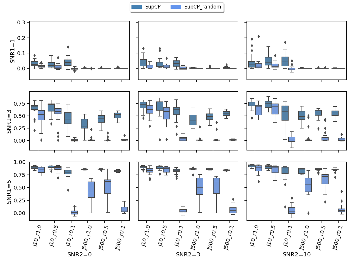
Refer to caption
Figure 7: Reconstruction evaluation of the underlying signal tensor using different initializations in SupCP, measured by the correlations. In each subplot, x axis label indicates different JJ and observing rate, the y axis is the achieved correlation, and the box colors represent different methods. The corresponding subplot column/row name represents the signal-to-noise ratio SNR1/SNR2.

C.2 Signal reconstruction on missing entries

Fig.8 compares the achieved correlations with the signal tensor using different methods, but only on those missing entries. The proposed strategy shows a clear gain in the setting of high missing rate or weak signal. Consistent with Fig.1, SPACO improves over SPACO- with high SNR2, and is much better than SupCP or CP when the signal size SNR1 is weak (but still estimable using SPACO) or when the missing rate is high.
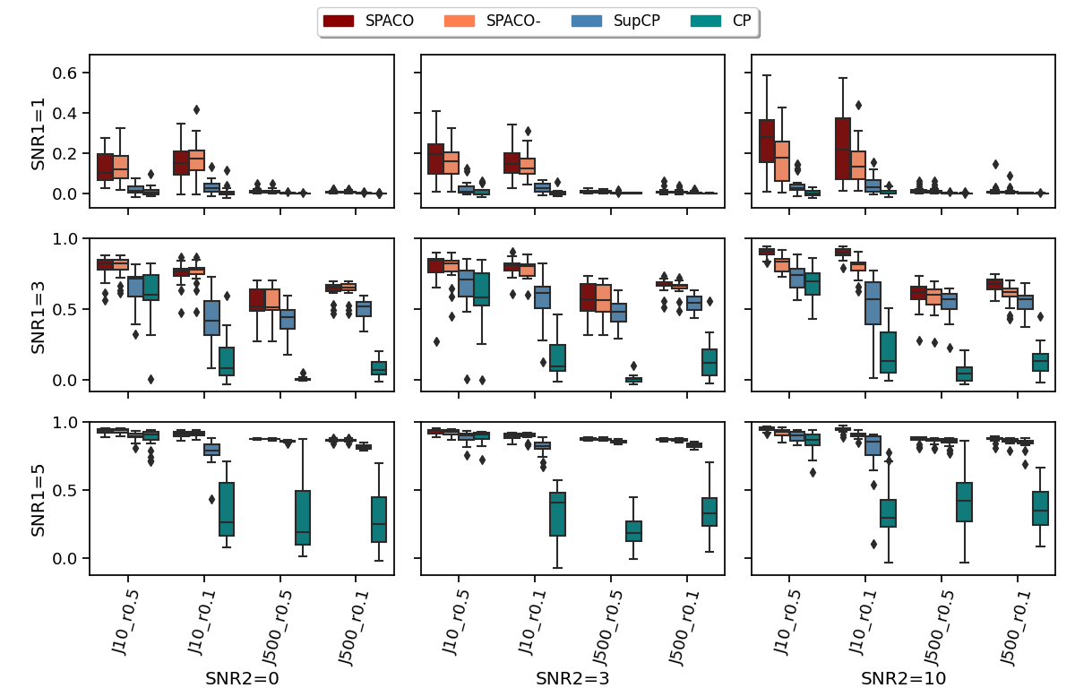
Refer to caption
Figure 8: Reconstruction evaluation on missing entries by the correlations between the estimates and the true signal tensor. In each subplot, x axis label indicates different JJ and observing rate, the y axis is the achieved correlation, and the box colors represent different methods. The corresponding subplot column/row name represents the signal-to-noise ratio SNR1/SNR2.

C.3 Type I error with observing rate r=1.0,0.1r=1.0,0.1
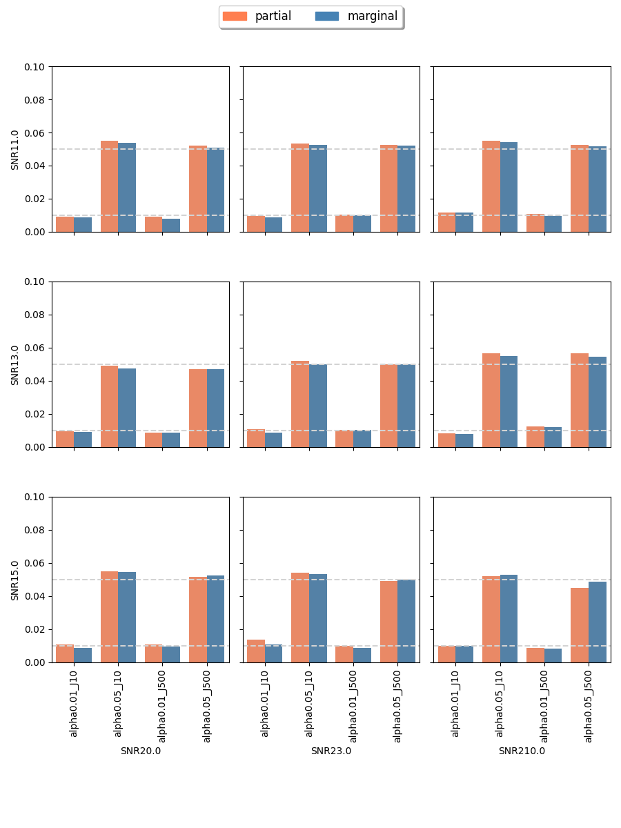
Figure 9: Achieved type I errors at observing rate r=1.0r=1.0. In each subplot, x axis label indicates different combination of feature dimension JJ and targeted level α{0.01,0.05}\alpha\in\{0.01,0.05\}, the y axis is the achieved type I errors. Different bar colors represent different tests (partial or marginal). The two dashed horizontal lines indicate levels 0.01 and 0.05.
Refer to caption
Figure 10: Achieved type I errors at observing rate r=0.1r=0.1. In each subplot, x axis label indicates different combination of feature dimension JJ and targeted level α{0.01,0.05}\alpha\in\{0.01,0.05\}, the y axis is the achieved type I errors. Different bar colors represent different tests (partial or marginal). The two dashed horizontal lines indicate levels 0.01 and 0.05.
Refer to caption

C.4 empirical p-value: cross-fit vs naive fit

In this section, we show qq-plots of the negative log10(pvalue)\log_{10}(\rm{pvalue}) from the null hypotheses against its theoretical values from the uniform distribution. In Fig.11-Fig.13, we show the results from observing rate r=1.0,0.5,0.1r=1.0,0.5,0.1 respectively, and the red/blue points represent those from the cross fit and the full fit with blue diagonal representing the expected theoretical behavior. The sub-title indicates the dimensionality JJ, observing rate r{1.0,0.5,0.1}r\in\{1.0,0.5,0.1\} and the type of estimate: partial_fitted means p values from partial independence test with p-value estimated using nct distribution and marginal_fitted means p values from marginal independence test with p-value estimated using nct distribution. The number of randomization used here is B=200B=200. We observe that direct plug-in of model parameters from full fit leads to poor performance when the signal-to-noise ratio is low. When SNR1=1=1, the log pvalue is severely inflated based on the full fit, the cross-fit provides much uniform null p-value distribution even with only a five-step update.
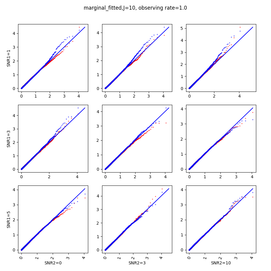
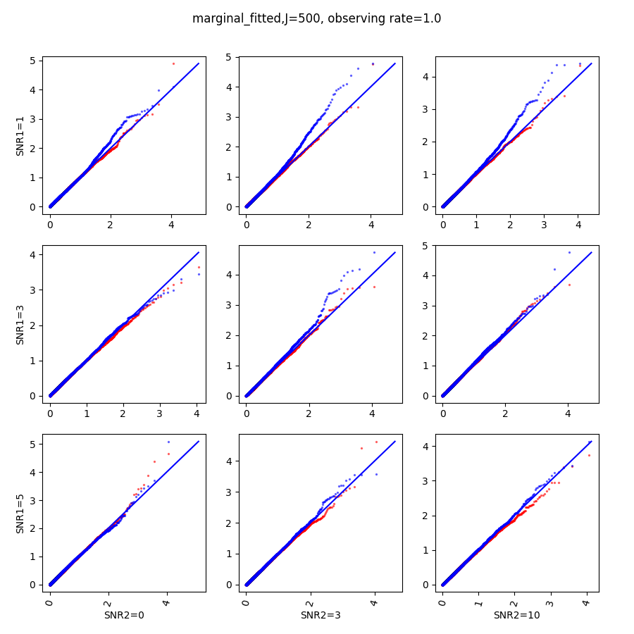
Figure 11: qq-plots of constructed p-values at r=1.0r=1.0. The p values are estimated with nct distribution. The red/blue points represent those from the cross-fit and the naive procedure, with blue diagonal representing the expected theoretical behavior.
Refer to caption
Refer to caption
Refer to caption
Refer to caption
Figure 12: qq-plots of constructed p-values at r=0.5r=0.5. The p values are estimated with nct distribution. The red/blue points represent those from the cross-fit and the naive procedure, with blue diagonal representing the expected theoretical behavior.
Refer to caption
Refer to caption
Refer to caption
Refer to caption
Figure 13: qq-plots of constructed p-values at r=0.1r=0.1. The p values are estimated with nct distribution. The red/blue points represent those from the cross-fit and the naive procedure, with blue diagonal representing the expected theoretical behavior.
Refer to caption
Refer to caption
Refer to caption
Refer to caption

When B=200B=200, the non-parametric estimate of the p values has a lower bound of 1B+1=1201\frac{1}{B+1}=\frac{1}{201}, but the nct-estimated p values do not have such a restriction. Fig.14 shows the non-parametric p value estimates at r=1.0r=1.0, we can easily show that the nct-estimated version provides more details for small p-values.
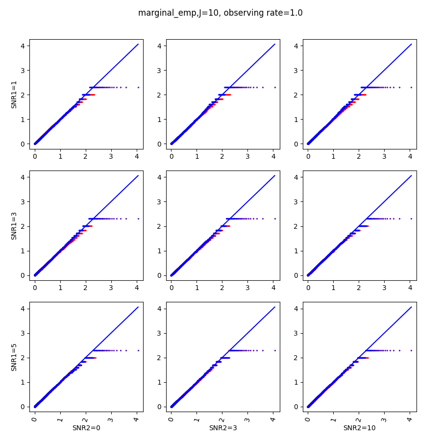
Figure 14: qq-plots of constructed p-values at r=1.0r=1.0. The p values are estimated directly from the empirical distribution. The red/blue points represent those from the cross-fit and the naive procedure, with blue diagonal representing the expected theoretical behavior.
Refer to caption
Refer to caption
Refer to caption
Refer to caption

References

  • Acar and Yener (2008) Acar, E. and B. Yener (2008). Unsupervised multiway data analysis: A literature survey. IEEE transactions on knowledge and data engineering 21(1), 6–20.
  • Argelaguet et al. (2018) Argelaguet, R., B. Velten, D. Arnol, S. Dietrich, T. Zenz, J. C. Marioni, F. Buettner, W. Huber, and O. Stegle (2018). Multi-omics factor analysis—a framework for unsupervised integration of multi-omics data sets. Molecular systems biology 14(6), e8124.
  • Bai and Wang (2016) Bai, J. and P. Wang (2016). Econometric analysis of large factor models. Annual Review of Economics 8, 53–80.
  • Besse and Ramsay (1986) Besse, P. and J. O. Ramsay (1986). Principal components analysis of sampled functions. Psychometrika 51(2), 285–311.
  • Bro and Andersson (1998) Bro, R. and C. A. Andersson (1998). Improving the speed of multiway algorithms: Part ii: Compression. Chemometrics and intelligent laboratory systems 42(1-2), 105–113.
  • Candès et al. (2018) Candès, E., Y. Fan, L. Janson, and J. Lv (2018). Panning for gold:‘model-x’knockoffs for high dimensional controlled variable selection series b statistical methodology.
  • Carroll et al. (1980) Carroll, J. D., S. Pruzansky, and J. B. Kruskal (1980). Candelinc: A general approach to multidimensional analysis of many-way arrays with linear constraints on parameters. Psychometrika 45(1), 3–24.
  • De Lathauwer et al. (2000) De Lathauwer, L., B. De Moor, and J. Vandewalle (2000). A multilinear singular value decomposition. SIAM journal on Matrix Analysis and Applications 21(4), 1253–1278.
  • Dempster et al. (1977) Dempster, A. P., N. M. Laird, and D. B. Rubin (1977). Maximum likelihood from incomplete data via the em algorithm. Journal of the Royal Statistical Society: Series B (Methodological) 39(1), 1–22.
  • Fan et al. (2008) Fan, J., Y. Fan, and J. Lv (2008). High dimensional covariance matrix estimation using a factor model. Journal of Econometrics 147(1), 186–197.
  • Fan et al. (2011) Fan, J., Y. Liao, and M. Mincheva (2011). High dimensional covariance matrix estimation in approximate factor models. Annals of statistics 39(6), 3320.
  • Harshman and Lundy (1994) Harshman, R. A. and M. E. Lundy (1994). Parafac: Parallel factor analysis. Computational Statistics & Data Analysis 18(1), 39–72.
  • Hinrich and Mørup (2019) Hinrich, J. L. and M. Mørup (2019). Probabilistic tensor train decomposition. In 2019 27th European Signal Processing Conference (EUSIPCO), pp.  1–5. IEEE.
  • Huang et al. (2008) Huang, J. Z., H. Shen, A. Buja, et al. (2008). Functional principal components analysis via penalized rank one approximation. Electronic Journal of Statistics 2, 678–695.
  • Imaizumi and Hayashi (2017) Imaizumi, M. and K. Hayashi (2017). Tensor decomposition with smoothness. In International Conference on Machine Learning, pp. 1597–1606. PMLR.
  • Katsevich and Roeder (2020) Katsevich, E. and K. Roeder (2020). Conditional resampling improves sensitivity and specificity of single cell crispr regulatory screens. bioRxiv.
  • Lam et al. (2011) Lam, C., Q. Yao, and N. Bathia (2011). Estimation of latent factors for high-dimensional time series. Biometrika 98(4), 901–918.
  • Li et al. (2016) Li, G., H. Shen, and J. Z. Huang (2016). Supervised sparse and functional principal component analysis. Journal of Computational and Graphical Statistics 25(3), 859–878.
  • Lock and Li (2018) Lock, E. F. and G. Li (2018). Supervised multiway factorization. Electronic journal of statistics 12(1), 1150.
  • Lucas et al. (2020) Lucas, C., P. Wong, J. Klein, T. B. Castro, J. Silva, M. Sundaram, M. K. Ellingson, T. Mao, J. E. Oh, B. Israelow, et al. (2020). Longitudinal analyses reveal immunological misfiring in severe covid-19. Nature 584(7821), 463–469.
  • Mnih and Salakhutdinov (2007) Mnih, A. and R. R. Salakhutdinov (2007). Probabilistic matrix factorization. Advances in neural information processing systems 20, 1257–1264.
  • Phan et al. (2013) Phan, A.-H., P. Tichavskỳ, and A. Cichocki (2013). Candecomp/parafac decomposition of high-order tensors through tensor reshaping. IEEE transactions on signal processing 61(19), 4847–4860.
  • Rendeiro et al. (2020) Rendeiro, A. F., J. Casano, C. K. Vorkas, H. Singh, A. Morales, R. A. DeSimone, G. B. Ellsworth, R. Soave, S. N. Kapadia, K. Saito, et al. (2020). Longitudinal immune profiling of mild and severe covid-19 reveals innate and adaptive immune dysfunction and provides an early prediction tool for clinical progression. medRxiv.
  • Sidiropoulos et al. (2017) Sidiropoulos, N. D., L. De Lathauwer, X. Fu, K. Huang, E. E. Papalexakis, and C. Faloutsos (2017). Tensor decomposition for signal processing and machine learning. IEEE Transactions on Signal Processing 65(13), 3551–3582.
  • Sorkine et al. (2004) Sorkine, O., D. Cohen-Or, Y. Lipman, M. Alexa, C. Rössl, and H.-P. Seidel (2004). Laplacian surface editing. In Proceedings of the 2004 Eurographics/ACM SIGGRAPH symposium on Geometry processing, pp.  175–184.
  • Tibshirani (2011) Tibshirani, R. (2011). Regression shrinkage and selection via the lasso: a retrospective. Journal of the Royal Statistical Society: Series B (Statistical Methodology) 73(3), 273–282.
  • Tipping and Bishop (1999) Tipping, M. E. and C. M. Bishop (1999). Probabilistic principal component analysis. Journal of the Royal Statistical Society: Series B (Statistical Methodology) 61(3), 611–622.
  • Wang et al. (2019) Wang, D., X. Liu, and R. Chen (2019). Factor models for matrix-valued high-dimensional time series. Journal of econometrics 208(1), 231–248.
  • Wang et al. (2021) Wang, D., Y. Zheng, H. Lian, and G. Li (2021). High-dimensional vector autoregressive time series modeling via tensor decomposition. Journal of the American Statistical Association, 1–19.
  • Yao et al. (2005) Yao, F., H.-G. Müller, and J.-L. Wang (2005). Functional data analysis for sparse longitudinal data. Journal of the American statistical association 100(470), 577–590.
  • Yokota et al. (2016) Yokota, T., Q. Zhao, and A. Cichocki (2016). Smooth parafac decomposition for tensor completion. IEEE Transactions on Signal Processing 64(20), 5423–5436.