Smooth convergence to the enveloping cylinder for mean curvature flow of complete graphical hypersurfaces

Wolfgang Maurer funded by the Deutsche Forschungsgemeinschaft (DFG, German Research Foundation) Project number 336454636

Abstract

For a mean curvature flow of complete graphical hypersurfaces $M_{t}=\mathop{\mathrm{graph}}u(\cdot,t)$ defined over domains $\Omega_{t}$ , the enveloping cylinder is $\partial\Omega_{t}\times\mathbb{R}$ . We prove the smooth convergence of $M_{t}-h\,e_{n+1}$ to the enveloping cylinder under certain circumstances. Moreover, we give examples demonstrating that there is no uniform curvature bound in terms of the inital curvature and the geometry of $\Omega_{t}$ . Furthermore, we provide an example where the hypersurface increasingly oscillates towards infinity in both space and time. It has unbounded curvature at all times and is not smoothly asymptotic to the enveloping cylinder. We also prove a relation between the initial spatial asymptotics at the boundary and the temporal asymptotics of how the surface vanishes to infinity for certain rates in the case $\Omega_{t}$ are balls.

1 Introduction

Mean curvature flow is the evolution of a hypersurface that moves with normal velocity equal to the mean curvature. It is described by a particularly appealing geometric evolution equation for the embedding ( $\frac{\mathrm{d}}{\mathrm{d}t}X=\Delta_{t}X$ ), while it is also the negative $L^{2}$ -gradient flow of the area functional.

For hypersurfaces $M_{t}$ that are the graphs of function $u(\cdot,t)$ , they solve mean curvature flow if and only if $u$ solves the quasilinear parabolic partial differential equation

\dot{u}=\left(\delta^{ij}-\frac{u^{i}\,u^{j}}{1+|\nabla u|^{2}}\right)u_{ij}\,.

(We make use of Einstein summation convention.) This equation has been extensively studied. To name a few of these works, that are in line with the present article, the author would like to mention [10], where the case of boundary values on a bounded domain is considered, [5], where the long-time existence of solutions for entire graphs is proven, and [19], where complete graphical hypersurfaces are considered. In the case of complete graphs, the representing functions $u(\cdot,t)$ are defined on open subsets $\Omega_{t}\subset\mathbb{R}^{n}$ and they diverge to infinity toward the boundary $\partial\Omega_{t}$ such that no boundary values occur and the graphs of $u(\cdot,t)$ are in fact complete hypersurfaces. The domains $\Omega_{t}$ must be time dependent in this setting and it turns out that they, or respectively their boundaries $\partial\Omega_{t}$ , form a weak solution of mean curvature flow. This can be understood by the following heuristic. The hypersurfaces $\mathop{\mathrm{graph}}u(\cdot,t)$ are in some sense asymptotic to the cylinder $\partial\Omega_{t}\times\mathbb{R}$ . Therefore, mean curvature flow is also expected for $\partial\Omega_{t}\times\mathbb{R}$ , and hence for $\partial\Omega_{t}$ because the $\mathbb{R}$ -factor does not contribute to the mean curvature or the evolution by mean curvature flow.

The main aim of this article is to prove that $\mathop{\mathrm{graph}}u(\cdot,t)$ is smoothly asymptotic to the cylinder $\partial\Omega_{t}\times\mathbb{R}$ under certain assumptions. For initially bounded curvature and bounded $\Omega_{0}$ the asymptotic is smooth for positive times $t>0$ as long as $\partial\Omega_{t}$ is not singular. It seems to be difficult to apply the method of proof, which relies on local graphical representations and pseudolocality, past singularities. Therefore, we investigate the case of noncollapsed mean curvature flow with a different method (the curvature bound of [9]) that allows going beyond singularities. So for the noncollapsed mean curvature flow of complete graphs the smooth asymptotics holds generally (still assuming initially bounded curvature).

If one drops the assumption of an initial curvature bound, the asymptotic may not be smooth anymore. We provide an interesting example where the asymptotic is non-smooth at any time and instead the graphical hypersurfaces infinitely sheets towards the enveloping cylinder. For the purpose of the construction we explicitely construct a barrier function which is defined over a shrinking annulus. This barrier allows for an estimate of $u$ in terms of the value of $u$ on a surrounding annulus earlier in time. Using this estimate we can prove that there are solutions $u$ over a shrinking ball $\Omega_{t}$ for which $\dot{u}(0,t)$ oscillates infinitely such that there are sequences $t_{k}\to T$ and $\tau_{k}\to T$ with $\dot{u}(0,t_{k})\to+\infty$ and $\dot{u}(0,\tau_{k})\to-\infty$ . The example shows that complicated kinds of singularities can appear at infinity for complete graphical hypersurfaces.

The barrier can also be used to prove a relationship between the spatial asymptotic of $u(x,0)$ as $x\to\partial\Omega_{0}$ and the temporal asymptotic $u(0,t)$ as $t\to T$ for rotationally symmetric graphs. In this context it is mandatory to mention [14, 15] where examples of rotationally symmetric, complete, graphical surfaces with a continuous spectrum of blow-up rates are constructed. The blow-up rates in their examples were intimately connected to the spatial asymptotics, too.

The article is organized as follows. Firstly, we will review the mean curvature flow of complete graphical hypersurfaces, because it is central to this paper and to set up the notation. In Section 3, we prove the smooth asymptotics to the enveloping cylinder up to the first singularity for initially bounded curvature. A curvature bound above some height is central to the proof. Despite this curvature bound above a height, we include in this section a sequence of examples demonstrating that there is no uniform curvature bound (independent of height) depending only on the initial curvature bound and the geometry of $\Omega_{t}$ . In Section 4, we prove the smooth asymptotics for noncollapsed mean curvature flows of complete graphs. The section also provides a construction establishing existence for such flows. Section 5 is devoted to the barrier over an annulus and its applications. The appendix contains invaluable information about normal graphs and noncollapsed mean curvature flow as well as weak mean curvature flows.

The author thanks O. Schnürer for posing the question discussed here and for his supervision of the authors PhD-thesis, where this work originates from. The author is also very grateful for the conversations, stimulations and for O. Schnürer’s patience.

2 Recapitulation of mean curvature flow without singularities

Since this paper builds on the ideas and results of “Mean curvature flow without singularities” ([19]), it is worthwhile to summarize the main points of [19]. This section does not contain new results. (We follow [19], or [17] when we diverge from [19].) Instead, it helps setting the notation and allows us to shorten our exposition lateron when similar steps as here are needed to be taken.

Mean curvature flow without singularities is mainly about the mean curvature flow of complete graphical hypersurfaces.

1.

Initial Data: Let $\Omega_{0}\subset\mathbb{R}^{n}$ be open and let $u_{0}\colon\Omega_{0}\to\mathbb{R}$ be a locally Lipschitz-continuous function. We assume that there is a continuous extension $\overline{u}_{0}\colon\mathbb{R}^{n}\to\overline{\mathbb{R}}=[-\infty,\infty]$ of $u_{0}$ such that $\{x:-\infty<\overline{u}_{0}(x)<\infty\}=\Omega_{0}$ and $\overline{u}_{0}|_{\Omega_{0}}=u_{0}$ hold.
2.

Solution Data: A mean curvature flow without singularities is a pair $(u,\Omega)$ of an relatively open subset $\Omega\subset\mathbb{R}^{n}\times[0,\infty)$ and a continuous function $u\colon\Omega\to\mathbb{R}$ . The zero time slice of $\Omega$ is supposed to be $\Omega_{0}$ , in line with a consistent notation $\Omega_{t}$ for the time slices ( $\Omega=\bigcup_{t\geq 0}\Omega_{t}\times\{t\}$ ). Moreover, we suppose that $u(\cdot,0)=u_{0}$ holds. For this reason, we call $(u_{0},\Omega_{0})$ the initial data for $(u,\Omega)$ .

Maximality condition: We suppose that there exists a continuous function $\overline{u}\colon\mathbb{R}^{n}\times[0,\infty)\to\overline{\mathbb{R}}$ such that $\{(x,t):-\infty<\overline{u}(x,t)<\infty\}=\Omega$ and $u|_{\Omega}=u$ hold.

Equation: The function $u$ is supposed to be smooth and to satisfy the equation of graphical mean curvature flow on $\Omega\setminus(\Omega_{0}\times\{0\})$ , i.e.,

(1) $\partial_{t}u=\left(\delta^{ij}-\frac{u^{i}\,u^{j}}{1+|Du|^{2}}\right)u_{ij}\;.$
3.

Hypersurfaces: We denote by $M_{t}\coloneqq\mathop{\mathrm{graph}}u(\cdot,t)$ the graphical hypersurfaces that move by their mean curvature (locally in a classical sense).
4.

Shadow flow: The family $(\Omega_{t})_{t\geq 0}$ is called the shadow flow.

Theorem 1.

For any such initial data $(u_{0},\Omega_{0})$ , there exists a corresponding mean curvature flow without singularities $(u,\Omega)$ . The shadow flow is a weak solution of mean curvature flow in dimension $n-1$ in a sense explained below (Remark 2 (3)).

Remark 2.

1.

The maximality condition implies $|u(x,t)|\to\infty$ for $(x,t)\to\partial\Omega$ . ( $\partial\Omega$ denotes the relative boundary of $\Omega$ in $\mathbb{R}^{n}\times[0,\infty)$ .) In particular, the hypersurfaces $M_{t}$ are complete. Moreover, the maximality condition implies that the solution is maximal in $t$ ; stopping the flow at an arbitrary time may prevent the maximality condition to hold.

The maximality condition is defined slightly differently in [19]. Only positive and proper functions $u$ are considered there. We follow [17] here, where these assumptions are dropped to some extent and the maximality condition is adapted accordingly.
2.

Although $M_{t}$ is smooth, the formalism allows for changes of the topology of $M_{t}$ . Singularities of $\partial\Omega_{t}$ may be interpreted as singularities of $M_{t}$ at infinity.
3.

In [19], the shadow flow is advertised as a weak solution. They underpin this by showing that (for their solution) $(\Omega_{t})_{t\in[0,\infty)}$ coincides with the level-set flow starting from $\Omega_{0}$ $\mathcal{H}^{n}$ -almost everywhere if the level-set flow is non-fattening.

In [17], for an arbitrary solution $(u,\Omega)$ the shadow flow is interpreted as a weak solution in the sense of a domain flow (cf. Definition 25).

Discussion of the proof of Theorem 1.

One constructs an approximating sequence of functions $v_{k}\colon\mathbb{R}^{n}\times[0,\infty)\to\overline{\mathbb{R}}$ . It needs to satisfy the following form of local equicontinuity: For any $a\in\mathbb{R}$ , any $R\in\mathbb{R}$ , and any $\varepsilon>0$ there is $\delta=\delta(a,R,\varepsilon)>0$ and an index $K=K(a,R,\varepsilon)\in\mathbb{N}$ such that for any $k\geq K$ and any $(x,s),(y,t)\in\mathbb{R}^{n}\times[0,\infty)$ with $|x|<R$ , $|v_{k}(x,s)|<a$ , and $|x-y|+|s-t|<\delta$ we have $|v_{k}(x,s)-v_{k}(y,t)|<\varepsilon$ . A variation on the Arzelà-Ascoli theorem then shows that a subsequence of $(v_{k})_{k\in\mathbb{N}}$ converges pointwise to a continuous function $\overline{u}\colon\mathbb{R}^{n}\times[0,\infty)\to\overline{\mathbb{R}}$ . We set $\Omega\coloneqq\{(x,t):-\infty<\overline{u}(x,t)<\infty\}$ and $u\coloneqq\overline{u}|_{\Omega}$ . The convergence is locally uniform on $\Omega$ .

To be approximating, the sequence needs to satisfy $v_{k}(\cdot,0)\to\overline{u}_{0}$ pointwise, where $\overline{u}_{0}$ is the above extension of the initial function such that $\overline{u}(\cdot,0)=\overline{u}_{0}$ holds. Furthermore, for any $a,R\in\mathbb{R}$ and any $t_{0}>0$ , we suppose that there is an index $K=K(a,R,t_{0})$ such that $v_{k}$ is a smooth solution of (1) on the set $\{(x,t):|v_{k}(x,t)|<a,\,|x|<R,\,t_{0}<|t|<R\}$ . Moreover, we assume uniform estimates of the form $|\partial^{\alpha}v_{k}|\leq C(\alpha,a,R,t_{0})$ for $k\geq K$ and for all multi-indices $\alpha$ on this set. The subsequential convergence $v_{k}\to u$ is then locally smooth on $\Omega\setminus(\Omega_{0}\times\{0\})$ . As a consequence, $u$ solves (1) on $\Omega\setminus(\Omega_{0}\times\{0\})$ and is as asserted.

We have summarized how one obtains a solution from an approximating sequence and what are sufficient conditions on this sequence. One still has to find the approximating sequence and prove the local estimates on the functions and its derivatives. For the approximations one could either solve initial boundary value problems or use the flow of closed hypersurfaces which have graphical parts. These are just two options and one cannot say in general how to approximate; it depends on the given problem.

For example, we can find an approximating sequence in the following way. One considers for $a\in\mathbb{R}_{+}$ the functions $\varphi_{a}\colon\overline{\mathbb{R}}\to\mathbb{R}$ with

(2)

\varphi_{a}(x)\coloneqq\begin{cases}x&|x|<a,\\ a&x\geq a,\\ -a&x\leq-a.\end{cases}

Then one mollifies $\varphi_{a}\circ\overline{u}$ and restricts to a ball. Solving graphical mean curvature flow on this ball with this initial function and holding the boundary values fixed over time, we find an approximator. (It can be extended to all of $\mathbb{R}^{n}$ by an arbitrary value.) An approximating sequence is obtained by taking increasingly larger $a$ , finer mollification parameter, and larger balls.

For the local estimates it is often possible to use the height function to construct a cut-off function.

We don’t say anything about the shadow flow here because the details of that part of the proof are not important to us. ∎

3 Curvature bounds for mean curvature flow of complete graphs

In this section we give hypothesis that render the heuristics rigorous that for a mean curvature flow without singularities $(u,\Omega)$ , the graph of $u(\cdot,t)$ and $\partial\Omega_{t}\times\mathbb{R}$ behave alike in sufficient heights. The first section, however, lowers our expectations towards a curvature bound for mean curvature flow of complete graphs.

3.1 Impossibility of a controlled curvature bound

In the title of this paragraph, one would need to explain what is meant by “controlled”. The issue is, what quantities is the curvature bound allowed to depend on? We will only allow the geometry of $\Omega_{t}$ and the initial curvature here. We cannot exclude curvature bounds that depend on more elaborate quantities.

We are going to construct a sequence of examples with uniformly bounded initial curvature over a domain which is a shrinking ball. Nevertheless, the curvature in these examples becomes arbitrarily large at some fixed time before the ball disappears. This demonstrates that there is no uniform curvature bound for the mean curvature flow without singularities that depends only on the initial curvature and the geometry of $\Omega_{t}$ .

We start with $\Omega_{0}=B_{1}(0)\subset\mathbb{R}^{2}$ . Every solution $(u,\Omega)$ of the mean curvature without singularities has $\Omega$ resemble the shrinking ball solution, which exists up to the time $t=\frac{1}{2}$ when $u$ vanishes to infinity. We start with an initial $u_{0}$ that is sketched in Figure 1. The torus shown in that figure is assumed to close at time $t=\frac{1}{4}$ when moved by its mean curvature. The mean curvature flow without singularities $M_{t}$ stays a smooth graph. So by the avoidance principle $M_{t}$ must have already passed through the torus by the time the torus closes. Now consider a sequence of initial surfaces $M_{0}$ that look essentially the same but have their tip further and further downstairs. These surfaces can be constructed such that their curvature is uniformly bounded among all of them. But at time $t=\frac{1}{4}$ , the tips must have passed through the torus. For this reason, the speeds of the tips must become arbitrarily large because they have to travel increasing distances in the same time. That means the mean curvature becomes arbitrarily large. We conclude that controlling the curvature of $M_{0}$ and the geometry of $\Omega_{t}$ is not sufficient to deduce a curvature bound for $M_{t}$ at later times.

Refer to caption — Figure 1: The torus closes and the solution must have passed through before.

In this counterexample sequence the problem does not arise from infinity. In fact, there everything is well-behaved. Furthermore, none of the members of the sequence actually has unbounded curvature. Therefore, we will keep the hypothesis of initially bounded curvature and of controlled geometry of $\Omega_{t}$ , but we will weaken the assertion. We will only obtain an uncontrolled curvature bound. In accordance with the fact that in our counterexample sequence the problem does not come from infinity, we obtain that under those hypothesis the solution $M_{t}$ is smoothly asymptotic to the cylinder $\Omega_{t}\times\mathbb{R}$ .

3.2 Smooth asymptotics to the cylinder

For interior curvature estimates we rely on the pseudolocality of mean curvature flow. This remarkable property of mean curvature flow means that one has control on solutions by means of local data; the behavior of the solution far out is irrelevant for that control. This is not to be confused with locality because a change far out will have effects everywhere, but these are mild enough such that estimates can still be derived from local data. This should be contrasted to the heat equation, where one can realize any given temperature after any given time at any given point in a room by making the walls of the room sufficiently hot.

We use the interior curvature estimates from [2], but one could also use [16], which is based on the pseudolocality theorem in [13], in conjunction with [5].

Theorem 3.

There exist $0<\varepsilon\leq 1$ and $L>0$ with the following property. Let $r>0$ . Let $(M_{t})_{0\leq t\leq T}$ be a smooth solution of mean curvature flow which is properly embedded in $B_{r}(x_{0})$ with $x_{0}\in M_{0}$ and such that $M_{0}$ is graphical in $B_{r}(x_{0})$ with gradient bounded by $L$ . Then the second fundamental form is estimated by

(3)

|A(x,t)|^{2}\leq\frac{1}{t}+(\varepsilon\,r)^{-2}

for $t\in(0,\min\{(\varepsilon r)^{2},T\}]$ and $x\in B_{\varepsilon r}(x_{0})\cap M_{t}$ .

If, in addition, the second fundamental form of $M_{0}\cap B_{r}(x_{0})$ is bounded by $r^{-1}$ , then

(4)

|A(x,t)|^{2}\leq(\varepsilon\,r)^{-2}

holds for $t\in[0,\min\{(\varepsilon r)^{2},T\}]$ and $x\in B_{\varepsilon r}(x_{0})\cap M_{t}$ .

Theorem 4.

Let $(u,\Omega)$ be a solution of the mean curvature flow without singularities. Suppose that $({\partial}{\Omega}_{t})_{0\leq t\leq T}$ is a smooth and compact solution of the mean curvature flow in dimension $n-1$ for some $T>0$ . Moreover, suppose $M_{0}$ has bounded curvature.

Then $M_{t}-h\,e_{n+1}$ converges for $0<t\leq T$ in $C_{\mathrm{loc}}^{\infty}$ to the cylinder $\partial\Omega_{t}\times\mathbb{R}$ for $h\to\infty$ . In particular, $\sup\limits_{x\in M_{t}}|A|^{2}(x,t)$ is bounded for $0\leq t\leq T$ .

Remark.

Instead of bounded curvature, one can assume that $M_{0}$ admits local graph representations of some radius $r$ with small Lipschitz constant (cf. Definition 17). Then the curvature of $M_{t}$ is bounded for small positive times by Theorem 3.

Proof of Theorem 4.

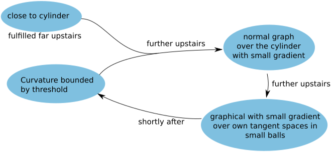
Firstly, we are going to prove a curvature estimate above some height. The asymptotic behavior is then treated afterwards. The idea for the curvature estimate is to alternately use Theorem 3, which provides a curvature estimate from a local graph representation, and that a curvature estimate ensures graph representations, as we are going to explain below. These two complement each other perfectly if done carefully. Essential is that the curvature is below a certain threshold $C_{A}$ so that we can ensure graph representations. Theorem 3 then supplies us with a curvature bound a small, but fixed, time later. If this bound is below $C_{A}$ , we can then repeat the argument. The rough idea is depicted in Figure 2.

We set $Z_{t}\coloneqq\partial\Omega_{t}\times\mathbb{R}$ .

Let $0<\varepsilon$ , $L\leq 1$ be as in Theorem 3. By Proposition 18 there is $r>0$ dependent on

L,\quad\sup_{t\in[0,T]}\sup_{x\in Z_{t}}|A_{Z_{t}}(x,t)|\,,\quad\text{and}\quad\sup_{t\in[0,T]}\sup_{x,y\in Z_{t}}\frac{\mathrm{dist}_{Z_{t}}(x,y)}{|x-y|}

with the following property. If $M$ is any normal graph over $Z_{t}$ with gradient bounded by $L/6$ and which is in a tubular neighborhood of thickness at most half of the maximal tubular neighborhood thickness, then $M$ admits local graph representations of radius $r$ with gradient bounded by $L$ . By decreasing $r$ if necessary, we may assume $r<1$ and $\sup_{M_{0}}|A|\leq r^{-1}$ , where $|A|$ corresponds to $M_{0}$ .

We set $C_{A}\coloneqq 2(\varepsilon\,r)^{-1}$ . This will function as a threshold for the curvature. By Corollary 20 there is $\delta>0$ such that for any two hypersurfaces $M^{\prime}\subset M$ , where $M^{\prime}$ has buffer $1$ in $M$ , with curvature bounded by $C_{A}$ and which lie in a (tubular) neighborhood of $Z_{t}$ of size $\delta$ , can be locally written as a normal graph over $Z_{t}$ with gradient bounded by $L/8$ .

We set

a\coloneqq\sup\{u(x,t)\colon t\in[0,T],\,x\in\Omega_{t},\,\mathrm{dist}(x,\partial\Omega_{t})\geq\delta\}\;,

such that $M_{t}^{a}\coloneqq M_{t}\cap\{x^{n+1}>a\}$ lies in a tubular neighborhood of $Z_{t}$ of size $\delta$ . By Lemma 21, $M_{t}^{a+1}$ is a normal graph over $Z_{t}$ (following Definition 14, where it can be a graph over a subset) if the curvature of $M_{t}^{a}$ is bounded by $C_{A}$ . By our choice of $r$ in the beginning of the proof, this shows that $M_{t}^{a+1}$ admits local graph representations of radius $r$ with gradient bound $L$ if $M_{t}^{a}$ ’s curvature is bounded by $C_{A}$ .

Because of $\sup_{M_{0}}|A|\leq r^{-1}<C_{A}$ , $M_{0}^{a+1}$ admits local graph representations of radius $r$ with gradient bounded by $L$ . The interior estimate (4) yields

(5)

|A(x,t)|^{2}\leq(\varepsilon\,r)^{-2}<(C_{A})^{2}

for $t\in[0,\min\{(\varepsilon r)^{2},T\}]$ and $x\in M_{t}^{a+1+r}\subset M_{t}^{a+2}$ .

From (3) we infer that, in the case that the curvature of $M_{t}^{a^{\prime}}$ ( $a^{\prime}\geq a$ ) is smaller than $C_{A}$ and, therefore, $M_{t}^{a^{\prime}+1}$ admits local graph representations of radius $r$ , like it is demonstrated above, the estimate

(6)

\big{|}A\big{(}x,t+(\varepsilon\,r)^{2}\big{)}\big{|}^{2}\leq 2\,(\varepsilon\,r)^{-2}<(C_{A})^{2}

holds for $x\in M_{t+(\varepsilon\,r)^{2}}^{a^{\prime}+2}$ .

Starting from the bound (5) on the interval $[0,\varepsilon^{2}\,r^{2}]\cap[0,T]$ , the estimate (6) can be applied iteratively to show that the curvature of $M_{t}^{a+2N}$ ( $N$ is some controlled number of steps) cannot reach the threshold $C_{A}$ for any $t\in[0,T]$ . The procedure is demonstrated in Figure 3. Starting with the curvature at the brown dot, (5) establishes the curvature bound depicted by the brown line. Since the curvature stays below the threshold $C_{A}$ , we can apply the curvature bound (6) to obtain the curvature bound in red. In fact, the picture even shows how to obtain (6) from (3). Starting from the red curvature bound, which is below the threshold $C_{A}$ , one can again apply (6) to obtain the orange curvature bound. In this way, we proceed through all the colors of the rainbow (and beyond). We will reach the time $T$ in finitely many steps, providing us with curvature estimates on the whole time interval. However, the region where the estimates hold go up in height by 2 units per step.

Below the height $a+2N$ the curvature is bounded (in a non-controlled fashion) because it is a continuous function on a compact set.

Now that we have curvature estimates, we can work on improving them: Because of the curvature bound, in great heights the solution $M_{t}$ is $C^{1}$ -close to the cylinder $Z_{t}$ . This follows from Lemma 21. We translate the solutions downwards, so we consider $M_{t}-h\,e_{n+1}$ , and by the Arzelà-Ascoli-Theorem we can extract a limit for $h\to\infty$ which must be the enveloping cylinder $Z_{t}$ . For $t>0$ , the convergence is not only uniform ( $C^{0}$ ) but by interior estimates for $|\nabla^{k}A|$ , that hold for mean curvature flows of bounded curvature [5], and interpolation inequalities the uniform convergence expands to smooth convergence. In other words, the solution $M_{t}$ is smoothly asymptotic to the cylinder $Z_{t}$ . ∎

Remark.

In the dimensions $n=1,2$ , the result holds beyond singularities: One can obtain the smooth convergence of $M_{t}-h\,e_{n+1}$ to the cylinder $\partial\Omega_{t}\times\mathbb{R}$ for all positive times $t>0$ provided $\partial\Omega_{t}$ is not singular. We are assuming that $\Omega_{0}$ is smooth and bounded.

In the case $n=1$ , $\Omega_{0}$ is a union of bounded intervals with fixed distances between them and $\Omega_{0}=\Omega_{t}$ holds for all times. Thus, there are no singular times and $M_{t}$ is smoothly asymptotic to $\partial\Omega_{t}\times\mathbb{R}$ for all $t>0$ .

In the case $n=2$ , the Gage-Hamilton-Grayson theorem [7, 8] ensures that any singularity of $(\partial\Omega_{t})_{t}$ looks like a shrinking circle when magnified. Therefore, the connected component of $\partial\Omega_{t}$ on which the singularity appears becomes extinct in that singularity. The proof of Theorem 4 can be carried out on each connected component of $\partial\Omega_{t}$ separately. And none of the connected components have seen singularities in their past. Loosely speaking, when a singularity arises, all problems related to it disappear in that singularity.

4 $\alpha$ -noncollapsed mean curvature flow without singularities

4.1 Asymptotics to the cylinder

Let $(u,\Omega)$ be a mean curvature flow without singularities with $u\geq 0$ . We note that $u(x,t)\to\infty$ as $(x,t)\to\partial\Omega$ . We assume that $\Omega$ is bounded. In particular, any $\Omega_{t}\subset\mathbb{R}^{n}$ is bounded and $\Omega_{t}=\emptyset$ for all $t\geq T$ with some $T>0$ . Furthermore, we suppose that $\Omega_{0}$ is smooth, mean convex, and $\alpha$ -noncollapsed for some $\alpha>0$ (Definition 32). We also assume that $u_{0}=u(\cdot,0)$ is smooth, that $M_{0}$ has bounded curvature, and that $M_{t}=\mathop{\mathrm{graph}}u|_{\Omega_{t}}$ is mean convex and $\alpha$ -noncollapsed for all $t\geq 0$ (if $M_{t}\neq\emptyset$ ).

Our aim in this section is to prove

Theorem 5.

With the above assumptions, if $\partial\Omega_{t}\subset\mathbb{R}^{n}$ is a smooth hypersurface for some $t>0$ then $M_{t}-h\,e_{n+1}$ converges in $C_{\textrm{loc}}^{\infty}$ to the cylinder $\partial\Omega_{t}\times\mathbb{R}$ for $h\to\infty$ .

Like in section 3, establishing a curvature bound is crucial. We exploit the $H$ -dependent curvature bound from Corollary 35. Firstly, we will use it to demonstrate that the mean curvature $H$ behaves continuously at infinity and converges to the mean curvature of $\partial\Omega_{t}$ (Theorem 6). Once we have control on $H$ , we can directly use the $H$ -dependent estimates to bound all the terms $|\nabla^{k}A|$ , $k\in\mathbb{N}$ , for $M_{t}$ .

Proof of Theorem 5.

Let $t>0$ be a time when $\partial\Omega_{t}$ is smooth. Theorem 6 asserts that $H[u](\cdot,t)$ is continuous with boundary values $H[\partial\Omega_{t}]$ (see Theorem 6 for the terminology). The continuity of $H[u](\cdot,t)$ , the compactness of $\overline{\Omega}_{t}$ , and the boundedness of $H[\partial\Omega_{t}]$ together imply the boundedness of $H[u](\cdot,t)$ and therefore the boundedness of the mean curvature $H$ of $M_{t}$ .

Because $M_{t}$ belongs to an $\alpha$ -noncollapsed mean curvature flow, Corollary 35 implies that the whole geometry of $M_{t}$ is bounded, i.e., all terms $|\nabla^{l}A|$ ( $l=0,1,\ldots$ ) are bounded. This applies even for times slightly before. The smooth convergence now follows from Lemma 21, the theorem of Arzelà-Ascoli, and interpolation inequalities. ∎

Theorem 6.

Let $H[u](\cdot,t)$ be the mean curvature of the graph of $u(\cdot,t)$ defined as a function on $\Omega_{t}$ . Then $H[u]$ is continuously extendable to $\overline{\Omega}$ with values in $(0,\infty]$ , and there holds $H[u](x,t)=H[\partial\Omega_{t}](x)$ for $x\in\partial\Omega_{t}$ with $H[\partial\Omega_{t}]$ the mean curvature of the boundary $\partial\Omega_{t}\subset\mathbb{R}^{n}$ (may be infinite).

Proof.

We denote the spacetime track by

(7)

\mathcal{M}\coloneqq\bigcup_{t\in[0,\infty)}M_{t}\times\{t\}\subset\mathbb{R}^{n+1}\times[0,\infty)\;.

In what follows, unspecified geometric quantities refer to $M_{t}$ . Points on $M_{t}$ are tracked in time along the normal direction.

We have

(8)

|\nabla H|=|g^{ij}\,\nabla_{k}h_{ij}|\leq|g^{ij}|\cdot|\nabla_{k}h_{ij}|=\sqrt{n}\,|\nabla A|

and

(9)

|\partial_{t}H|=\big{|}\Delta H+|A|^{2}\,H\big{|}\leq|g^{ij}|\cdot|g^{kl}|\cdot|\nabla_{ij}^{2}h_{kl}|+|A|^{2}\cdot|g^{kl}|\cdot|h_{kl}|=n\,|\nabla^{2}A|+\sqrt{n}\,|A|^{3}\;.

Thus, by Lemma 7 and these inequalities, $|A_{\mathcal{M}}|^{2}$ is bounded by terms of the form $\frac{|\nabla^{l}A|^{2}}{(1+H^{2})^{l+1}}$ with $l=0,1,2$ . By virtue of Corollary 35, the curvature of the spacetime track $\mathcal{M}$ is uniformly bounded for $t\geq t_{0}>0$ . For times $0<t<t_{0}$ , $t_{0}$ sufficiently small, we may use Theorem 4 to see that $\mathcal{M}$ has bounded curvature for these times, too.

By assumption every $M_{t}$ is $\alpha$ -noncollapsed and because $M_{t}$ is not a hyperplane we have $H>0$ everywhere. Because $H$ is the normal speed, this implies that the spacetime track $\mathcal{M}$ is graphical over $\mathbb{R}^{n+1}$ in the time direction. More precisely, the domain is $D\coloneqq\{(x,y)\in\mathbb{R}^{n+1}\colon y\geq u_{0}(x)\}$ . The representation function is the time of arrival function $\tau\colon D\to\mathbb{R}$ . By the $\alpha$ -noncollapsedness of the $M_{t}$ and because of the boundedness of interior balls, the mean curvature is uniformly bounded from below, $H\geq c>0$ . This implies that $|\nabla\tau|$ is uniformly bounded. Together with the curvature bound for $\mathcal{M}=\mathop{\mathrm{graph}}\tau$ , this implies a finite bound for $\|\tau\|_{C^{2}}$ .

The sequence of functions $\tau(x,y+h)$ is monotonically increasing and, by the $C^{2}$ -bound, converges for $h\to\infty$ in $C_{\mathrm{loc}}^{1}$ to a $C^{1,1}$ function $\sigma$ defined on $\Omega_{0}\times\mathbb{R}$ . It is independent of the $y$ -variable and represents $\partial\Omega\times\mathbb{R}$ as a graph.

The mean curvature depends on the gradient of the time of arrival function:

(10)

H[u](x,t)=\left|\nabla\tau(x,u(x,t))\right|^{-1}\,.

For $(x,t)\to\partial\Omega$ we have $u(x,t)\to\infty$ and therefore

(11)

H[u](x,t)=\left|\nabla\tau(x,u(x,t))\right|^{-1}\to\left|\nabla\sigma(x,0)\right|^{-1}=H[\partial\Omega_{t}](x)\;.\qed

Remark.

From the proof one can easily see that $\partial\Omega\in C^{1,1}$ holds.

Remark.

It is worth mentioning that, in contrast to $|A_{\mathcal{M}}|$ , $|\nabla A_{\mathcal{M}}|$ can not be estimated by terms of the form $\frac{|\nabla^{l}A|^{2}}{(1+H^{2})^{l+1}}$ . Therefore, we do not get higher estimates for the spacetime track from Corollary 35.

Lemma 7.

The squared norm of the second fundamental form of the spacetime track $\mathcal{M}$ is given by

(12)

|A_{\mathcal{M}}|^{2}=\frac{|A|^{2}}{1+H^{2}}+2\,\frac{|\nabla H|^{2}}{(1+H^{2})^{2}}+\frac{|\partial_{t}H|^{2}}{(1+H^{2})^{3}}

where the geometric quantities on the right hand side correspond to those of $M_{t}$ .

Proof.

For a point $(x_{0},y_{0},t_{0})\in\mathcal{M}$ ( $x_{0}\in\mathbb{R}^{n}$ , $y_{0}\in\mathbb{R}$ ) we represent $\mathcal{M}$ locally as the graph of a function $v(x,t)$ . By a rotation in $(x,y)$ -space ( $\mathbb{R}^{n+1}$ ) we may assume that $\nabla_{x}v(x_{0},t_{0})=0$ holds. Because $(M_{t})_{t}$ is a mean curvature flow, $v$ solves graphical mean curvature flow, i.e., $\partial_{t}v=\sqrt{1+|\nabla_{x}v|^{2}}\,H$ holds. At the point $(x_{0},t_{0})$ we obtain $\partial_{t}v=H$ , $\nabla_{x}\partial_{t}v=\nabla_{x}H$ , and $\partial_{t}^{2}v=\partial_{t}H$ . Before stating computations with these identities at $(x_{0},y_{0},t_{0})$ , let us briefly fix some notation: $\mathrm{D}_{x}f$ is a linear form and $\nabla_{x}f$ is the gradient of $f$ , which is given by $\nabla_{x}f=g^{-1}\cdot(\mathrm{D}_{x}f)^{\mathsf{T}}$ .

	$\displaystyle h_{\mathcal{M}}$	$\displaystyle=\frac{\mathrm{D}_{(x,t)}^{2}v}{\sqrt{1+\|\nabla_{(x,t)}v\|^{2}}}=\frac{1}{\sqrt{1+\|(0,H)\|^{2}}}\begin{pmatrix}\mathrm{D}_{x}^{2}v&(\mathrm{D}_{x}\partial_{t}v)^{\mathsf{T}}\\ \mathrm{D}_{x}\partial_{t}v&\partial_{t}^{2}v\end{pmatrix}$
		$\displaystyle=\frac{1}{\sqrt{1+H^{2}}}\begin{pmatrix}h&(\mathrm{D}_{x}H)^{\mathsf{T}}\\ \mathrm{D}_{x}H&\partial_{t}H\end{pmatrix}$
	$\displaystyle g_{\mathcal{M}}^{-1}$	$\displaystyle=\left(\left(\delta^{\alpha\beta}\right)-\frac{\nabla_{(x,t)}v\otimes\nabla_{(x,t)}v}{1+\|\nabla_{(x,t)}v\|^{2}}\right)=\begin{pmatrix}\left(\delta^{ij}\right)&0\\ 0&1-\frac{H^{2}}{1+H^{2}}\end{pmatrix}=\begin{pmatrix}g^{-1}&0\\ 0&\frac{1}{1+H^{2}}\end{pmatrix}$
	$\displaystyle A_{\mathcal{M}}$	$\displaystyle=g_{\mathcal{M}}^{-1}\cdot h_{\mathcal{M}}=\frac{1}{\sqrt{1+H^{2}}}\begin{pmatrix}g^{-1}\cdot h&g^{-1}\cdot(\mathrm{D}_{x}H)^{\mathsf{T}}\\ \frac{\mathrm{D}_{x}H}{1+H^{2}}&\frac{\partial_{t}H}{1+H^{2}}\end{pmatrix}$
		$\displaystyle=\frac{1}{\sqrt{1+H^{2}}}\begin{pmatrix}A&\nabla_{x}H\\ \frac{\mathrm{D}_{x}H}{1+H^{2}}&\frac{\partial_{t}H}{1+H^{2}}\end{pmatrix}$
	$\displaystyle\|A_{\mathcal{M}}\|^{2}$	$\displaystyle=\textrm{tr}(A_{\mathcal{M}}^{2})=\frac{1}{1+H^{2}}\mathrm{tr}\begin{pmatrix}A^{2}+\nabla_{x}H\cdot\frac{\mathrm{D}_{x}H}{1+H^{2}}&A\cdot\nabla_{x}H+\nabla_{x}H\cdot\frac{\partial_{t}H}{1+H^{2}}\\ \frac{\mathrm{D}_{x}H}{1+H^{2}}\cdot A+\frac{\partial_{t}H}{1+H^{2}}\,\frac{\mathrm{D}_{x}H}{1+H^{2}}&\frac{\mathrm{D}_{x}H}{1+H^{2}}\cdot\nabla_{x}H+\left(\frac{\partial_{t}H}{1+H^{2}}\right)^{2}\end{pmatrix}$
		$\displaystyle=\frac{1}{1+H^{2}}\left(\|A\|^{2}+2\,\frac{\|\nabla_{x}H\|^{2}}{1+H^{2}}+\frac{(\partial_{t}H)^{2}}{(1+H^{2})^{2}}\right)\;.\qed$

4.2 Construction of an $\alpha$ -noncollapsed mean curvature flow without singularities

Under the presumption that $\Omega_{0}$ is bounded and smooth, $H[\partial\Omega_{0}]>0$ , $|A_{M_{0}}|\leq C$ , and $H_{M_{0}}\geq c>0$ , we will construct a mean curvature flow without singularities that is $\alpha$ -noncollapsed for some $\alpha>0$ and matches these data. Theorem 5 from the last section tells us that this flow is smoothly asymptotic to the cylinder $\partial\Omega_{t}\times\mathbb{R}$ for all times $t$ when $\partial\Omega_{t}$ is smooth.

At first, we describe our approach. We approximate $M_{0}$ by closed hypersurfaces. This is done in a way such that these approximating hypersurfaces are $\alpha$ -noncollapsed. We let flow these by the level-set flow. By the results of [9], the $\alpha$ -noncollapsedness persists along this flow with the same $\alpha$ . The level-set flow will in fact be a smooth graphical flow below a certain height. This height tends in the limit of the approximation to infinity. We can then employ a limit process to obtain a mean curvature flow without singularities which is $\alpha$ -noncollapsed.

Approximation of $M_{0}$ by compact $M_{0}^{\delta}$ .

Let $\delta>0$ (to be thought of being small). The initial surface $M_{0}$ is above a height $a_{\delta}=\max\{u_{0}(x)\colon x\in\Omega_{0},\,\mathrm{dist}(x,\partial\Omega_{0})\geq\delta\}$ in a $\delta$ -neighborhood of $N\coloneqq\partial\Omega_{0}\times\mathbb{R}$ . If $\delta$ is sufficiently small, then Lemma 21 yields that $M_{0}$ is a normal graph over $N$ above the height $a_{\delta}$ (according to our Definition 14 we also speak of a normal graph over $N$ if we have a graph over a subset of $N$ ). Let $v$ be the representation function for this normal graph. We note that we always choose the outward pointing normal. But because we define the tubular diffeomorphism in the form $(p,d)\mapsto p-d\,\nu$ , the function $v$ is positive (cf. Definitions 13 and 14). We have $v=\mathcal{O}(\delta)$ , $|\nabla v|=\mathcal{O}(\sqrt{\delta})$ , and $|\nabla^{2}v|\leq C$ . By Proposition 15 there hold

(13)		$\displaystyle g_{M_{0}}$	$\displaystyle=g_{N}+\mathcal{O}(\delta)$
(14)		$\displaystyle h_{M_{0}}$	$\displaystyle=h_{N}+\nabla^{2}v+\mathcal{O}(\delta)\;.$

We choose a smooth function $\lambda\equiv\lambda_{\delta}\colon\mathbb{R}\to[0,1]$ with $\lambda(x)=0$ for $x\leq a_{\delta}$ and $\lambda(x)=1$ for $x\geq a_{\delta}+\frac{1}{\delta}$ . We can engineer this function in such a way that on $(a_{\delta},a_{\delta}+\frac{1}{\delta})$ we have $\lambda^{\prime}>0$ and that $|\lambda^{\prime}|+|\lambda^{\prime\prime}|^{1/2}=\mathcal{O}(\delta)$ holds. By slight abuse of notation, $\lambda$ becomes a function on $N$ as $\lambda(x^{n+1})$ .

On $N\cap\{a_{\delta}<x^{n+1}\leq a_{\delta}+\frac{2}{\delta}\}$ we define for $0<\varepsilon<\delta^{3}$

(15)

w\coloneqq(1-\lambda)\,v+\lambda\,\frac{\varepsilon}{2}\left(a_{\delta}+\frac{2}{\delta}-x^{n+1}\right)^{2}.

Then we have

(16)	$\displaystyle\begin{split}\nabla_{e_{n+1}}w&=(1-\lambda)\,\nabla_{e_{n+1}}v+\lambda\,\varepsilon\left(x^{n+1}-\left(a_{\delta}+\frac{2}{\delta}\right)\right)\\ &\quad+\lambda^{\prime}\left(\frac{\varepsilon}{2}\left(a_{\delta}+\frac{2}{\delta}-x^{n+1}\right)^{2}-v\right),\end{split}$
(17)	$\displaystyle\nabla_{\partial\Omega_{0}}w$	$\displaystyle=(1-\lambda)\,\nabla_{\partial\Omega_{0}}v\;,$
(18)	$\displaystyle\nabla_{\partial\Omega_{0}}^{2}w$	$\displaystyle=(1-\lambda)\,\nabla_{\partial\Omega_{0}}^{2}v\;,$
(19)	$\displaystyle\nabla_{\partial\Omega_{0}}\nabla_{e_{n+1}}w$	$\displaystyle=\nabla_{e_{n+1}}\nabla_{\partial\Omega_{0}}w=(1-\lambda)\,\nabla_{\partial\Omega_{0}}\nabla_{e_{n+1}}v-\lambda^{\prime}\,\nabla_{\partial\Omega_{0}}v\;,$
(20)	$\displaystyle\begin{split}\nabla_{e_{n+1}}^{2}w&=(1-\lambda)\,\nabla_{e_{n+1}}^{2}v+\lambda\,\varepsilon+2\,\lambda^{\prime}\left(\varepsilon\left(x^{n+1}-\left(a_{\delta}+\frac{2}{\delta}\right)\right)-\nabla_{e_{n+1}}v\right)\\ &\quad+\lambda^{\prime\prime}\left(\frac{\varepsilon}{2}\left(a_{\delta}+\frac{2}{\delta}-x^{n+1}\right)^{2}-v\right)\;.\end{split}$

If $0<\varepsilon<\delta^{3}$ is sufficiently small (depending on $v$ ), we have $0<w<v$ , $\nabla w=(1-\lambda)\nabla v+\mathcal{O}(\delta)$ , and $\nabla^{2}w=(1-\lambda)\,\nabla^{2}v+\mathcal{O}(\delta)$ on $N\cap\{a_{\delta}<x^{n+1}\leq a_{\delta}+\frac{2}{\delta}\}$ .

Let $W$ be the hypersurface that is given as the normal graph over $N$ with representation function $w$ . Then, again by Proposition 15

(21)		$\displaystyle g_{W}$	$\displaystyle=g_{N}+\mathcal{O}(\delta)$
(22)		$\displaystyle\begin{split}h_{W}&=h_{N}+\nabla^{2}w+\mathcal{O}(\delta)=h_{N}+(1-\lambda)\,\nabla^{2}v+\mathcal{O}(\delta)\\ &=(1-\lambda)\,h_{M_{0}}+\lambda\,h_{N}+\mathcal{O}(\delta)\;.\end{split}$

Therefore, if we adjust the constants a little bit and choose $\delta$ sufficiently small, there hold $|A_{W}|^{2}\leq C$ and $H_{W}\geq c>0$ .

The compact approximation $M_{0}^{\delta}$ to $M_{0}$ is now constructed as follows: In the region $\{x^{n+1}\leq a_{\delta}\}$ , it coincides with $M_{0}$ . In the region $\{a_{\delta}<x^{n+1}\leq a_{\delta}+\frac{2}{\delta}\}$ , we set it equal to $W$ . From this part we obtain the part above the height $a_{\delta}+\frac{2}{\delta}$ by reflection at the hyperplane $\{x^{n+1}=a_{\delta}+\frac{2}{\delta}\}$ . By construction, $M_{0}^{\delta}$ is mirror-symmetrical. In fact, its interior is a vain set if $\varepsilon$ is chosen sufficiently small. This stems from the fact that then $\nabla_{e_{n+1}}w<0$ holds, which one can check from (16). Of course, $M_{0}^{\delta}$ is smooth and we have $|A_{M_{0}^{\delta}}|^{2}\leq C$ and $H_{M_{0}^{\delta}}\geq c>0$ .

Uniform $\alpha$ -noncollapsedness of the $M_{0}^{\delta}$ .

Lemma 8.

For $C>0$ , $c>0$ , and $r>0$ there is $\alpha>0$ such that: If a hypersurface $M$ has bounded second fundamental form $|A|\leq C$ , mean curvature $H\geq c$ , and admits local graph representations of radius $r$ , then $M$ is $\alpha$ -noncollapsed.

Proof.

Let $x\in M$ . Then, inside $B_{r}(x)$ , $M$ is a graph over $\textrm{T}_{x}M$ . Let $\rho\coloneqq\min\{\frac{r}{2},\,\frac{1}{C}\}$ . Then, the two closed balls $\overline{B}_{\rho}(x\pm\rho\,\nu(x))$ intersect $M$ only in $x$ . Thus, if we choose $\alpha\coloneqq c\,\rho$ , $x$ admits interior and exterior balls of radius $\frac{\alpha}{H(x)}\leq\frac{\alpha}{c}=\rho$ . Because $\alpha$ does not depend on $x$ , this demonstrates that $M$ is $\alpha$ -noncollapsed. ∎

To apply the lemma it remains to show that the $M_{0}^{\delta}$ admit local graph representations of a radius $r$ that is independent of $\delta$ . To this end, we realize that the $M_{0}^{\delta}$ are normal graphs over $\partial\Omega_{0}\times\mathbb{R}$ for the most part, with two “ $M_{0}$ -caps.” By Proposition 18 the normal graph part of each $M_{0}^{\delta}$ admits local graph representations of a controlled radius independent of $\delta$ . Therefore, Lemma 8 is applicable and yields an $\alpha>0$ such that the $M_{0}^{\delta}$ are $\alpha$ -noncollapsed.

Evolution of the $M_{0}^{\delta}$ and passing to a limit.

So far, we have constructed smooth closed hypersurfaces $M_{0}^{\delta}$ such that

•

$M_{0}^{\delta}$ coincides with $M_{0}$ below the height $a_{\delta}$ ,
•
•

the $M_{0}^{\delta}$ are mean convex and $\alpha$ -noncollapsed with $\alpha>0$ independent of $\delta$ ,
•

The $M_{0}^{\delta}$ are symmetric double graphs with respect to the hyperplanes $\{x:x^{n+1}=a_{\delta}+\frac{2}{\delta}\}$ in the sense of [18].

We can flow $M_{0}^{\delta}$ by the mean curvature flow as in [18]: Singularities only occur on the hyperplane $\{x:x^{n+1}=a_{\delta}+\frac{2}{\delta}\}$ and the surfaces stay symmetric double graphs. In particular, the part below the hyperplane is smooth and graphical.

By Proposition 29, the weak solution is unique. In particular, $(M_{t}^{\delta})_{t}$ coincides with the level-set flow. By Theorem 33, the level-set flow is $\alpha$ -noncollapsed for all $t\geq 0$ with the same $\alpha$ as for $M_{0}^{\delta}$ . Hence, $\left(M_{t}^{\delta}\right)_{t\in[0,\infty)}$ is $\alpha$ -noncollapsed.

We now may use the a priori estimates and the Arzelà-Ascoli argument as employed before in Section 2 to pass to a limit as we let $\delta\to 0$ . The limit is a smooth mean curvature flow $(M_{t})_{t}$ starting from $M_{0}$ that is graphical and provides us with a mean curvature flow without singularities $(u,\Omega)$ with initial value $(u_{0},\Omega_{0})$ . Clearly, the approximation outlined in Section 2 would have given us this result as well. But importantly, the uniform $\alpha$ -noncollapsedness of the approximators carries over to the limit because $M_{t}^{\delta}\to M_{t}$ locally smoothly, proving that $M_{t}$ is $\alpha$ -noncollapsed.

Thus, we have proven the following theorem.

Theorem 9.

Let $\Omega_{0}\subset\mathbb{R}^{n}$ be a bounded, smooth, and mean convex domain. Let $u_{0}\colon\Omega_{0}\to\mathbb{R}$ be a positive and smooth function such that $u_{0}(x)\to\infty$ for $x\to\partial\Omega_{0}$ . Let $M_{0}\coloneqq\mathop{\mathrm{graph}}u_{0}$ . We assume that there are constants $C,c>0$ such that $|A_{M_{0}}|\leq C$ and $H_{M_{0}}\geq c$ . Then there exists a mean curvature flow without singularities $(u,\Omega)$ with initial values $(u_{0},\Omega_{0})$ such that $(M_{t})_{t\in[0,\infty)}$ is $\alpha$ -noncollapsed for some $\alpha>0$ .

5 Barrier over annuli

In the present section we assume $n\geq 2$ .

Central to this section is a barrier which is defined over annuli. This barrier enables us to prove estimates for a mean curvature flow in terms of the height over an annulus earlier in time. This will be exploited to obtain various results.

The upper barrier has the following geometry (Fig. 4.1). Initially start with an annulus in $n$ -dimensional Euclidean space. Over this, we consider a special function which tends to infinity at the boundary of the annulus. As time goes by, the initial annulus shrinks by mean curvature flow and the function is adjusted accordingly to have the shrinking annulus as its domain; while at the same time, the function is shifted upwards.

In the first section, we will write down the barrier and prove that it really functions as a barrier. The upshot is Theorem 11. Afterwards, in the second section, we will utilize the barrier to construct an “ugly” example of mean curvature flow without singularities with wild oscillations which persist up to the vanishing time. As another application of the barrier, we will prove in the third section a certain relationship between the spatial asymptotics of a mean curvature flow without singularities and its temporal asymptotics at the vanishing time.

5.1 Construction of the barrier

The barrier construction starts with a hypersurface that is obtained from a grim reaper curve which is rotated around the $x^{n+1}$ -axis. The grim reaper is a well-known special solution of curve-shortening flow (one-dimensional mean curvature flow). It has the explicit graphical representation ( $\lambda>0$ )

(23)

u_{\mathrm{gr}}(x,t)=-\frac{1}{\lambda}\log\cos(\lambda\,x)+\lambda\,t\qquad\text{for }x\in\left(-\frac{\pi}{2\lambda},\frac{\pi}{2\lambda}\right),\;t\in\mathbb{R}\;.

In this form $\mathop{\mathrm{graph}}u_{\mathrm{gr}}$ translates with speed $\lambda$ upwards.

Our barrier construction is motivated by this solution and initially we start with a grim reaper curve rotated around a vertical axis. Let us have a look at the barrier function now:

(24)

w(x,t)=-\frac{1}{\lambda}\log\cos\left[\lambda\left(\sqrt{|x|^{2}+2(n-1)t}-R\right)\right]+\lambda\,t+f(t)\;,

where $R,\lambda>0$ . As can be seen, $w$ is similar to $u_{\mathrm{gr}}$ . But $x$ is replaced by the term $\sqrt{|x|^{2}+2(n-1)t}$ which is motivated by the radius of an $(n-1)$ -dimensional sphere flowing by its mean curvature. The function $f(t)$ will be adequately chosen to make $w$ satisfy the correct differential inequality. We will give two possible choices for $f$ , one rather simple, the other more elaborate but much smaller as $\lambda$ becomes large. However, we include the second one only for the sake of completeness because in our applications $\lambda\,t$ dominates $f(t)$ for large $\lambda$ in either case.

Before we start proving the differential inequality, we must talk about the domain of definition of $w$ . We set

(25)		$\displaystyle t\in I(R)\coloneqq[0,T(R)]\coloneqq\left[0,\frac{R^{2}}{2(n-1)}\right]$
(26)		$\displaystyle x\in A_{t}(R,\lambda)\coloneqq\left\{x\in\mathbb{R}^{n}\colon\left(R-\frac{\pi}{2\lambda}\right)<\sqrt{\|x\|^{2}+2(n-1)t}<\left(R+\frac{\pi}{2\lambda}\right)\right\}.$

$A_{t}(R,\lambda)$ is an annulus or a ball, depending on $t$ , $R$ , and $\lambda$ .

Differential inequality.

To keep the computations accessible, we will make the abbreviations $\sqrt{\rule{0.0pt}{4.30554pt}\quad}$ for $\sqrt{|x|^{2}+2(n-1)t}$ and $[\;\cdot\;]$ for $\lambda\left(\sqrt{\rule{0.0pt}{4.30554pt}\quad}-R\right)$ .

To show that $w$ is an upper barrier, we must prove

(27)

-\dot{w}+\left(\delta^{ij}-\frac{w^{i}w^{j}}{1+|\nabla w|^{2}}\right)w_{ij}\stackrel{{\scriptstyle!}}{{\leq}}0\;.

First, we determine the derivatives.

(28)	$\displaystyle\dot{w}$	$\displaystyle=\tan[\;\cdot\;]\,\frac{n-1}{\sqrt{\rule{0.0pt}{4.30554pt}\quad}}+\lambda+f^{\prime}(t)\;,$
(29)	$\displaystyle w_{i}$	$\displaystyle=\tan[\;\cdot\;]\,\frac{x_{i}}{\sqrt{\rule{0.0pt}{4.30554pt}\quad}}\;,$
(30)	$\displaystyle w_{ij}$	$\displaystyle=\lambda\left(1+\tan^{2}[\;\cdot\;]\right)\frac{x_{i}\,x_{j}}{\sqrt{\rule{0.0pt}{4.30554pt}\quad}^{2}}+\frac{\tan[\;\cdot\;]}{\sqrt{\rule{0.0pt}{4.30554pt}\quad}}\left(\delta_{ij}-\frac{x_{i}\,x_{j}}{\sqrt{\rule{0.0pt}{4.30554pt}\quad}^{2}}\right).$

Substituting into (27) yields

(31)

\begin{split}&-\dot{w}+\left(\delta^{ij}-\frac{w^{i}w^{j}}{1+|\nabla w|^{2}}\right)w_{ij}\\ &\quad=-\dot{w}+\frac{1}{1+|\nabla w|^{2}}\bigg{(}(1+|\nabla w|^{2})\delta^{ij}-w^{i}w^{j}\bigg{)}w_{ij}\\ &\quad=-\lambda-f^{\prime}(t)-\tan[\;\cdot\;]\,\frac{n-1}{\sqrt{\rule{0.0pt}{4.30554pt}\quad}}\\ &\qquad+\frac{\lambda\,(1+\tan^{2}[\;\cdot\;])}{1+\tan^{2}[\;\cdot\;]\frac{|x|^{2}}{\sqrt{\rule{0.0pt}{3.01389pt}\quad}^{2}}}\left(\left(1+\tan^{2}[\;\cdot\;]\frac{|x|^{2}}{\sqrt{\rule{0.0pt}{4.30554pt}\quad}^{2}}\right)\frac{|x|^{2}}{\sqrt{\rule{0.0pt}{4.30554pt}\quad}^{2}}-\tan^{2}[\;\cdot\;]\frac{|x|^{4}}{\sqrt{\rule{0.0pt}{4.30554pt}\quad}^{4}}\right)\\ &\qquad+\frac{\frac{\tan[\;\cdot\;]}{\sqrt{\rule{0.0pt}{3.01389pt}\quad}}}{1+\tan^{2}[\;\cdot\;]\frac{|x|^{2}}{\sqrt{\rule{0.0pt}{3.01389pt}\quad}^{2}}}\left(\left(1+\tan^{2}[\;\cdot\;]\frac{|x|^{2}}{\sqrt{\rule{0.0pt}{4.30554pt}\quad}^{2}}\right)\left(n-\frac{|x|^{2}}{\sqrt{\rule{0.0pt}{4.30554pt}\quad}^{2}}\right)\right.\\ &\hskip 128.0374pt\left.-\tan^{2}[\;\cdot\;]\left(\frac{|x|^{2}}{\sqrt{\rule{0.0pt}{4.30554pt}\quad}^{2}}-\frac{|x|^{4}}{\sqrt{\rule{0.0pt}{4.30554pt}\quad}^{4}}\right)\right)\\ &\quad=-\lambda-f^{\prime}(t)-\frac{\tan[\;\cdot\;]}{\sqrt{\rule{0.0pt}{4.30554pt}\quad}}(n-1)+\frac{\lambda\,(1+\tan^{2}[\;\cdot\;])}{1+\tan^{2}[\;\cdot\;]\frac{|x|^{2}}{\sqrt{\rule{0.0pt}{3.01389pt}\quad}^{2}}}\left(\frac{|x|^{2}}{\sqrt{\rule{0.0pt}{4.30554pt}\quad}^{2}}\right)\\ &\qquad+\frac{\frac{\tan[\;\cdot\;]}{\sqrt{\rule{0.0pt}{3.01389pt}\quad}}}{1+\tan^{2}[\;\cdot\;]\frac{|x|^{2}}{\sqrt{\rule{0.0pt}{3.01389pt}\quad}^{2}}}\left(\left(1+\tan^{2}[\;\cdot\;]\frac{|x|^{2}}{\sqrt{\rule{0.0pt}{4.30554pt}\quad}^{2}}\right)(n-1)+\left(1-\frac{|x|^{2}}{\sqrt{\rule{0.0pt}{4.30554pt}\quad}^{2}}\right)\right)\\ &\quad=-f^{\prime}(t)+\frac{\left(1-\frac{|x|^{2}}{\sqrt{\rule{0.0pt}{3.01389pt}\quad}^{2}}\right)}{1+\tan^{2}[\;\cdot\;]\frac{|x|^{2}}{\sqrt{\rule{0.0pt}{3.01389pt}\quad}^{2}}}\left(\frac{\tan[\;\cdot\;]}{\sqrt{\rule{0.0pt}{4.30554pt}\quad}}-\lambda\right)\stackrel{{\scriptstyle!}}{{\leq}}0\;.\end{split}

In the case $\frac{\tan[\;\cdot\;]}{\sqrt{\rule{0.0pt}{3.01389pt}\quad}}\leq\lambda$ , the inequality clearly holds. Thus, let us from now on assume $\frac{\tan[\;\cdot\;]}{\sqrt{\rule{0.0pt}{3.01389pt}\quad}}>\lambda$ .

Neglecting terms with the appropriate signs, we aim to show

(32)

\frac{\frac{\tan[\;\cdot\;]}{\sqrt{\rule{0.0pt}{3.01389pt}\quad}}}{1+\frac{\tan^{2}[\;\cdot\;]}{\sqrt{\rule{0.0pt}{3.01389pt}\quad}^{2}}|x|^{2}}\stackrel{{\scriptstyle!}}{{\leq}}f^{\prime}(t)\;.

If we can choose $f$ in such a way then the differential inequality (27) follows.

We are going to utilize the following lemma.

Lemma 10.

Let $J\subset\mathbb{R}_{>0}$ be an interval and $y\colon J\to\mathbb{R}_{>0}$ a monotonically increasing function, which is continuous and surjective. Then

(33)

\frac{y(r)}{1+y^{2}(r)\,r^{2}}\leq\frac{1}{a}

holds for all $r\in J$ , where $a$ is the unique solution of $y(a)=\frac{1}{a}$ .

Proof.

It is not hard to see that there is a unique solution $a$ of $y(a)=\frac{1}{a}$ given the hypothesis on $y$ .

We distinguish two cases. If $r\leq a$ holds, we find

(34)

\frac{y(r)}{1+y^{2}(r)\,r^{2}}\leq y(r)\leq y(a)=\frac{1}{a}\;.

In the case that $r>a$ holds, we have

(35)

\frac{y(r)}{1+y^{2}(r)\,r^{2}}\leq\frac{y(r)}{1+y^{2}(r)\,a^{2}}\;.

The expression $\frac{y}{1+y^{2}a^{2}}$ tends to $0$ for both $y\to 0$ and $y\to\infty$ . Hence, it attains its maximum at an interior point $b$ . We can determine $b$ from the extremality condition

(36)

0=\left.\frac{\mathrm{d}}{\mathrm{d}y}\left(\frac{y}{1+y^{2}a^{2}}\right)\right|_{y=b}=\frac{1+b^{2}a^{2}-2b^{2}a^{2}}{(1+b^{2}a^{2})^{2}}=\frac{1-b^{2}a^{2}}{(1+b^{2}a^{2})^{2}}\;.

We infer that $b=\frac{1}{a}$ is the maximum point. That leads to

(37)

\frac{y}{1+y^{2}a^{2}}\leq\frac{b}{1+b^{2}a^{2}}=\frac{1/a}{1+1}<\frac{1}{a}

for any $y\in\mathbb{R}_{>0}$ . Bringing together (35) and (37), the assertion follows. ∎

Application of the lemma.

We shall derive (32) with the help of Lemma 10. Clearly, $\frac{\tan[\;\cdot\;]}{\sqrt{\rule{0.0pt}{3.01389pt}\quad}}$ , seen as a function of $r\coloneqq|x|$ , will take the role of $y(r)$ . Notice that we fix $t\in I(R)$ here. The interval $J$ is appropriately chosen to be

(38)

J=\left(\sqrt{R^{2}-2(n-1)t},\sqrt{\left(R+\frac{\pi}{2\lambda}\right)^{2}-2(n-1)t}\right),

such that $[\;\cdot\;]\coloneqq\lambda(\sqrt{\rule{0.0pt}{4.30554pt}\quad}-R)\in(0,\frac{\pi}{2})$ . This makes $y(r)=\frac{\tan[\;\cdot\;]}{\sqrt{\rule{0.0pt}{3.01389pt}\quad}}$ well defined on $J$ and surjective onto $\mathbb{R}_{>0}$ .

Now we show, that our choice of $y$ is monotonically increasing. The derivative with respect to $\sqrt{\rule{0.0pt}{4.30554pt}\quad}$ is

(39)

\begin{split}\frac{\mathrm{d}}{\mathrm{d}\sqrt{\rule{0.0pt}{4.30554pt}\quad}}\frac{\tan[\lambda(\sqrt{\rule{0.0pt}{4.30554pt}\quad}-R)]}{\sqrt{\rule{0.0pt}{4.30554pt}\quad}}&=\frac{\lambda}{\sqrt{\rule{0.0pt}{4.30554pt}\quad}\,\cos^{2}[\;\cdot\;]}-\frac{\tan[\;\cdot\;]}{\sqrt{\rule{0.0pt}{4.30554pt}\quad}^{2}}=\frac{\lambda\sqrt{\rule{0.0pt}{4.30554pt}\quad}-\sin[\;\cdot\;]\cos[\;\cdot\;]}{\sqrt{\rule{0.0pt}{4.30554pt}\quad}^{2}\cos^{2}[\;\cdot\;]}\\ &\geq\frac{\lambda\sqrt{\rule{0.0pt}{4.30554pt}\quad}-[\;\cdot\;]}{\sqrt{\rule{0.0pt}{4.30554pt}\quad}^{2}\cos^{2}[\;\cdot\;]}=\frac{\lambda\,R}{\sqrt{\rule{0.0pt}{4.30554pt}\quad}^{2}\cos^{2}[\;\cdot\;]}>0\;.\end{split}

So $\frac{\tan[\;\cdot\;]}{\sqrt{\rule{0.0pt}{3.01389pt}\quad}}$ is increasing as a function of $\sqrt{\rule{0.0pt}{4.30554pt}\quad}$ . And because $\sqrt{\rule{0.0pt}{4.30554pt}\quad}$ is increasing in $r$ , $y(r)=\frac{\tan[\;\cdot\;]}{\sqrt{\rule{0.0pt}{3.01389pt}\quad}}$ is increasing in $r$ as well.

Finally, Lemma 10 is applicable and yields

(40)

\frac{\frac{\tan[\;\cdot\;]}{\sqrt{\rule{0.0pt}{3.01389pt}\quad}}}{1+\frac{\tan^{2}[\;\cdot\;]}{\sqrt{\rule{0.0pt}{3.01389pt}\quad}^{2}}\,|x|^{2}}\leq\frac{1}{a_{t}}\;,

where $a_{t}$ is the unique solution in $J$ of the equation

(41)

\frac{\tan\left[\lambda\left(\sqrt{a_{t}^{2}+2(n-1)t}-R\right)\right]}{\sqrt{a_{t}^{2}+2(n-1)t}}=\frac{1}{a_{t}}\;.

To further estimate $\frac{1}{a_{t}}$ in (40), we must extract information from (41). We will now demonstrate two possible ways to do so.

First choice for $f$ .

We notice that

(42)

\tan\left(\lambda\left(\sqrt{a_{t}^{2}+2(n-1)t}-R\right)\right)=\frac{\sqrt{a_{t}^{2}+2(n-1)t}}{a_{t}}\geq 1=\tan\left(\frac{\pi}{4}\right)\,.

Consequently, and by $2(n-1)t\leq R^{2}$ ,

(43)

a_{t}^{2}\geq\left(\frac{\pi}{4\lambda}+R\right)^{2}-2(n-1)t\geq\frac{\pi R}{2\lambda}\;.

Choosing

(44)

\boxed{f(t)\coloneqq\sqrt{\frac{2\lambda}{\pi R}}\;t}

we infer from (40) and (43)

(45)

\frac{\frac{\tan[\;\cdot\;]}{\sqrt{\rule{0.0pt}{3.01389pt}\quad}}}{1+\frac{\tan^{2}[\;\cdot\;]}{\sqrt{\rule{0.0pt}{3.01389pt}\quad}^{2}}\,|x|^{2}}\leq\frac{1}{a_{t}}\leq\sqrt{\frac{2\lambda}{\pi R}}=f^{\prime}(t)\;.

I.e., (32), and hence (27) hold.

Second choice for $f$ .

We write

(46)

s\coloneqq\sqrt{a_{t}^{2}+2(n-1)t}\;.

We note that $s$ depends on $t$ and lies in the range $\left[R+\tfrac{\pi}{4\lambda},R+\tfrac{\pi}{2\lambda}\right)$ , which can be seen from (42). With $s$ at hand we can rewrite (41) as

(47)

\frac{1}{a_{t}}=\frac{1}{\sqrt{s^{2}-2(n-1)t}}=\frac{\tan(\lambda\,(s-R))}{s}\;.

This can easily be solved for $2(n-1)t$ . We write $\tau(s)$ for $2(n-1)t$ viewed as a function of $s$ :

(48)

\tau(s)\coloneqq s^{2}\left(1-\frac{1}{\tan^{2}(\lambda(s-R))}\right),\qquad s\in\left[R+\tfrac{\pi}{4\lambda},\,R+\tfrac{\pi}{2\lambda}\right)\;.

We continuously extend $\tau$ to the closed interval through $\tau(R+\frac{\pi}{2\lambda})=(R+\frac{\pi}{2\lambda})^{2}$ . We will estimate $\tau(s)$ from below by

(49)

\sigma(s)\coloneqq\left(1-4\lambda\left(R+\frac{\pi}{2\lambda}\right)\right)s^{2}+4\lambda s^{3}\;;

$\sigma$ is the solution of $\sigma^{\prime}(s)=\frac{2}{s}\sigma(s)+4\lambda s^{2}$ with $\sigma\left(R+\tfrac{\pi}{2\lambda}\right)=\tau\left(R+\tfrac{\pi}{2\lambda}\right)=\left(R+\tfrac{\pi}{2\lambda}\right)^{2}$ . The function $\tau$ fulfills the differential inequality

(50)

\begin{split}\tau^{\prime}(s)&=2s\left(1-\frac{1}{\tan^{2}(\lambda\,(s-R))}\right)+2\lambda\,s^{2}\frac{1+\tan^{2}(\lambda\,(s-R))}{\tan^{3}(\lambda\,(s-R))}\\ &\leq\frac{2}{s}\tau(s)+4\lambda\,s^{2}\;.\end{split}

It follows that

(51)

\frac{\mathrm{d}}{\mathrm{d}s}(\tau(s)-\sigma(s))\leq\frac{2}{s}\tau(s)+4\lambda\,s^{2}-\left(\frac{2}{s}\sigma(s)+4\lambda\,s^{2}\right)=\frac{2}{s}(\tau(s)-\sigma(s))\;.

In fact the inequality is strict except for $s=R+\frac{\pi}{4\lambda}$ . Thus, whenever $\tau(s)=\sigma(s)$ for some $s\in(R+\frac{\pi}{4\lambda},R+\frac{\pi}{2\lambda})$ , we have $\tau^{\prime}(s)<\sigma^{\prime}(s)$ and there is an $\varepsilon>0$ such that $\tau>\sigma$ on $(s-\varepsilon,s)$ . Considering $\sup\{s\colon\tau(s)<\sigma(s)\}$ , it is now easy to show that $\tau\geq\sigma$ on the whole interval $\left[R+\frac{\pi}{4\lambda},\,R+\frac{\pi}{2\lambda}\right]$ . So we have shown for $s\in\left[R+\frac{\pi}{4\lambda},\,R+\frac{\pi}{2\lambda}\right]$

(52)	$\displaystyle\tau(s)$	$\displaystyle\geq\left(1-4\lambda\left(R+\frac{\pi}{2\lambda}\right)\right)s^{2}+4\lambda s^{3}\;,$
(53)	$\displaystyle\frac{\tau(s)}{\left(R+\frac{\pi}{4\lambda}\right)^{2}}$	$\displaystyle\geq\frac{\tau(s)}{s^{2}}\geq 1-4\lambda\left(R+\frac{\pi}{2\lambda}\right)+4\lambda\,s\;,$
(54)	$\displaystyle\begin{split}s&\leq R+\frac{\pi}{2\lambda}-\frac{1}{4\lambda}\left(1-\frac{\tau(s)}{\left(R+\frac{\pi}{4\lambda}\right)^{2}}\right)\\ &=R+\frac{1}{\lambda}\left(\frac{\pi}{2}-\frac{1}{4}\left(1-\frac{\tau(s)}{\left(R+\frac{\pi}{4\lambda}\right)^{2}}\right)\right).\end{split}$

Let us return to (46), the value for $s$ we are interested in. Let us also remember that $\tau(s)=2(n-1)t$ holds in this context. With $s\geq R+\frac{\pi}{4\lambda}$ and (54) we can continue from (47)

(55)

\frac{1}{a_{t}}\leq\frac{\tan(\lambda(s-R))}{s}\leq\frac{1}{R+\frac{\pi}{4\lambda}}\,\tan\left(\frac{\pi}{2}-\frac{1}{4}\left(1-\frac{2(n-1)t}{\left(R+\frac{\pi}{4\lambda}\right)^{2}}\right)\right).

We integrate the last term:

(56)

\boxed{f(t)\coloneqq\frac{2\left(R+\frac{\pi}{4\lambda}\right)}{n-1}\left[-\log\sin\left(\frac{1}{4}\left(1-\frac{2(n-1)t}{\left(R+\frac{\pi}{4\lambda}\right)^{2}}\right)\right)+\log\sin\left(\frac{1}{4}\right)\right].}

Then we obtain (32) from (55) and (40). So the differential inequality (27) for $w$ follows with this choice for $f$ .

Asymptotics of $f$ for large $\lambda$ .

The merit of the second choice for $f$ is the milder growth in $\lambda$ . While (44) clearly grows like $\sqrt{\lambda}$ , (56) only grows like $\log(\lambda)$ . To see this let us evaluate $f$ at the final time $T(R)$ of the time interval under consideration ( $T(R)\coloneqq\frac{R^{2}}{2(n-1)}$ ). Let $f_{1}$ be the first choice, (44), and let $f_{2}$ be the second, (56). Then we have

(57)

f_{1}(T(R))=\sqrt{\frac{2\lambda}{\pi\,R}}\;\frac{R^{2}}{2(n-1)}=\frac{R}{4(n-1)}\sqrt{\frac{8R\,\lambda}{\pi}}\;.

On the other hand, for $\lambda\to\infty$ :

(58)

\begin{split}f_{2}(T(R))&=\frac{2\left(R+\frac{\pi}{4\lambda}\right)}{n-1}\left[-\log\sin\left(\frac{1}{4}\frac{\left(R+\frac{\pi}{4\lambda}\right)^{2}-R^{2}}{\left(R+\frac{\pi}{4\lambda}\right)^{2}}\right)+\log\sin(\frac{1}{4})\right]\\ &\simeq-\frac{2R}{n-1}\;\log\sin\left(\frac{1}{4}\frac{\frac{\pi}{2\lambda}R}{R^{2}}\right)\\ &\simeq-\frac{2R}{n-1}\;\log\left(\frac{\pi}{8R\,\lambda}\right)\\ &=\frac{2R}{n-1}\;\log\left(\frac{8R\,\lambda}{\pi}\right)\;.\end{split}

Barrier property and annulus dependent estimate.

So far we have proven that for any choice of $f$ ((44) or (56)) $w$ fulfills the differential inequality (27) for all $t\in I(R)$ and $x\in A_{t}(R,\lambda)\setminus\{0\}$ . For this reason, a mean curvature flow cannot touch $\mathop{\mathrm{graph}}w(\cdot,t)$ from below at any interior point if the flow is disjoint initially. A special case, however, is the point $(0,w(0,t))$ (if defined) because $w$ does not solve (27) at $x=0$ . In fact, $w$ is not even differentiable at $x=0$ . But still, no smooth surface can touch $\mathop{\mathrm{graph}}w$ from below at $(0,w(0,t))$ : All of the directional derivatives of $w$ at zero are defined and they all are strictly negative, and hence there is not even a smooth curve, let alone a hypersurface, that can touch $w$ from below at that point.

It remains to exclude that $\mathop{\mathrm{graph}}w(\cdot,t)$ is crossed at infinity. Then $\mathop{\mathrm{graph}}w(\cdot,t)$ is a barrier and we obtain the following annulus dependent estimate.

Theorem 11.

Let $R,\lambda>0$ . Recall the definition of $A_{t}(R,\lambda)$ in (26). Let $(u,\Omega)$ be a solution of mean curvature flow without singularities in $\mathbb{R}^{n+1}$ ( $n\geq 2$ ). Suppose $A_{0}(R,\lambda)\Subset\Omega_{0}$ and

(59)

u(x,0)\leq-\frac{1}{\lambda}\log\cos\big{[}\lambda(|x|-R)\big{]}\qquad\text{ for all }x\in A_{0}(R,\lambda)\;.

Then for $t\in I(R)=[0,\frac{R^{2}}{2(n-1)}]$ there holds $A_{t}(R,\lambda)\Subset\Omega_{t}$ and

(60)

u(x,t)\leq w(x,t)=-\frac{1}{\lambda}\log\cos\left[\lambda\left(\sqrt{|x|^{2}+2(n-1)t}-R\right)\right]+\lambda\,t+f(t)

holds for all $x\in A_{t}(R,\lambda).$ The expression $f(t)$ can be given by (44) or (56) depending on your preferences.

Proof.

From [17] we know that $A_{t}(R,\lambda)\Subset\Omega_{t}$ for all $t>0$ , because the boundary of $A_{t}(R,\lambda)$ moves by mean curvature flow. In particular, $\mathop{\mathrm{graph}}u(\cdot,t)$ will not touch $\mathop{\mathrm{graph}}w(\cdot,t)$ at infinity. As we have demonstrated above, there will be no touching in the interior, either. Thus, (60) holds and the theorem is proven. ∎

Clearly $-w$ resembles a subsolution, and consequently, $\mathop{\mathrm{graph}}-w(\cdot,t)$ is a lower barrier which cannot be touched from above by any mean curvature flow.

5.2 Example with wild oscillations

We can use Theorem 11 to construct an example of mean curvature flow without singularities which behaves quite badly. The associated domain $\Omega$ simply describes a shrinking ball and the associated function $u$ converges to $+\infty$ at $\partial\Omega$ . So the graphical surface $M_{t}=\mathop{\mathrm{graph}}u(\cdot,t)$ vanishes at $+\infty$ the moment when $\Omega_{t}$ shrinks to a point. Special about the surface is that it does not vanish monotonically to infinity. Instead, $u(0,t)$ increasingly oscillates as $t$ approaches the final time. The surface $M_{t}$ has unbounded curvature at any time, a behavior that is not mirrored by the domain $\Omega_{t}$ . In fact, as we go upwards at a fixed time $t$ , $M_{t}$ has to get closer and closer to $\partial\Omega_{t}\times\mathbb{R}$ . However, $M_{t}$ is not smoothly asymptotic to $\partial\Omega_{t}\times\mathbb{R}$ but $M_{t}$ approaches $\Omega_{t}\times\mathbb{R}$ with more and more sheets. Figure 5 is an attempt to depict $M_{t}$ . For simplicity we will only consider the case $n=2$ , although it is straightforward to generalize to higher $n$ .

For all $k\in\mathbb{N}$ with $k\geq 2$ we define the Intervals $I_{k}\coloneqq\left(\frac{k-2}{k-1},\frac{k-1}{k}\right)$ . The length of $I_{k}$ is given by $\frac{1}{(k-1)k}$ . Let $\lambda_{k}\coloneqq(k-1)k\,\pi$ and let $R_{k}$ be the centers of the $I_{k}$ . Then we define

(61)		$\displaystyle w_{+}(x)$	$\displaystyle\coloneqq\begin{cases}-\frac{1}{\lambda_{k}}\log\cos\big{[}\lambda_{k}\,(\|x\|-R_{k})\big{]}+k&\text{for }\|x\|\in I_{k}\text{ with even }k,\\ +\infty&\text{else},\end{cases}$
(62)		$\displaystyle w_{-}(x)$	$\displaystyle\coloneqq\begin{cases}+\frac{1}{\lambda_{k}}\log\cos\big{[}\lambda_{k}\,(\|x\|-R_{k})\big{]}+k^{3}&\text{for }\|x\|\in I_{k}\text{ with odd }k,\\ -\infty&\text{else.}\end{cases}$

The functions $w_{\pm}$ are continuous and $w_{-}<w_{+}$ holds, in fact, even $w_{+}-w_{-}=\infty$ is true. Figure 6 sketches $w_{+}$ and $w_{-}$ . The different added constants $k$ and $k^{3}$ are there to ensure that the barriers corresponding to $w_{+}$ and $w_{-}$ stay interlocked for all times such that a mean curvature flow between those is bound to oscillate infinitely towards $\partial\Omega_{t}\times\mathbb{R}$ . But we are going to have a closer look at this now.

Let $u_{0}$ be any smooth function on $B_{1}(0)\subset\mathbb{R}^{2}$ with $w_{-}<u_{0}<w_{+}$ and with $u_{0}(x)\to\infty$ for $x\to\partial B_{1}(0)$ . Let $u\colon\Omega\to\mathbb{R}$ be a mean curvature flow without singularities that starts from $u_{0}$ . The solution is defined up to the time $T=\frac{1}{2}$ , at which the balls $\Omega_{t}$ shrink to a point.

Let $T_{k}\coloneqq\frac{R_{k}^{2}}{2}$ . Theorem 11 yields for even $k$

(63)

\begin{split}u(0,T_{k})&\leq k-\frac{1}{\lambda_{k}}\log\cos\left[\lambda_{k}\left(\sqrt{2T_{k}}-R_{k}\right)\right]+\left(\lambda_{k}+\sqrt{\frac{2\lambda_{k}}{\pi\,R_{k}}}\right)T_{k}\\ &=k+\left((k-1)\,k\,\pi+\sqrt{\frac{2(k-1)\,k}{R_{k}}}\right)T_{k}\\ &\simeq\frac{\pi}{2}\,k^{2}\qquad(k\to\infty)\;.\end{split}

Analogously, we obtain for odd $k$

(64)

\begin{split}u(0,T_{k})&\geq k^{3}-\left((k-1)\,k\,\pi+\sqrt{\frac{2(k-1)\,k}{R_{k}}}\right)T_{k}\\ &\simeq k^{3}\qquad(k\to\infty)\;.\end{split}

This says that $u(0,T_{2l+1})$ is larger than $\frac{1}{2}(2l+1)^{3}$ , while $u(0,T_{2l})$ is smaller than $2(2l)^{2}$ if the number $l\in\mathbb{N}$ is large enough. This shows that $u(0,t)$ has no clear rate with which it tends to infinity. Since $T_{k}\to\frac{1}{2}$ it also shows that $u(0,t)$ oscillates more and more on smaller and smaller time intervals and that there must be a sequence $(t_{k})_{k\in\mathbb{N}}$ of times with $t_{k}\to T=\frac{1}{2}$ and $\dot{u}(0,t_{k})\to-\infty$ , while it is clear that there are also sequences $(\tilde{t}_{k})_{k\in\mathbb{N}}$ with $\tilde{t}_{k}\to T$ and $\dot{u}(0,\tilde{t}_{k})\to+\infty$ . In summary, one can say that much of the behavior of $u_{0}$ for $|x|\to R=1$ is transmitted by virtue of Theorem 11 to $u(0,t)$ for $t\to T$ . In the next paragraph we will see more of this.

Remark.

An example of a mean curvature flow without singularities akin to the one we have discussed is defined on a half-space. It also has unbounded curvature for all $t\geq 0$ and it sheets towards a plane. It can be constructed in a similar fashion but instead of the annulus barrier one uses grim reapers cross $\mathbb{R}$ in that case.

5.3 Relation between spatial and temporal asymptotics

Theorem 11 shows that the height of a solution can be estimated by the height of the solution on an annulus at a prior time. This can be used to derive a relationship between temporal and spatial asymptotics.

Theorem 12.

Let $n\geq 2$ and let $u_{0}\colon\mathbb{R}^{n}\supset B_{\rho}(0)\to\mathbb{R}$ be a smooth function and suppose that there are $\alpha>1$ and $C>0$ such that

(65)

u_{0}(x)\simeq C\,(\rho-|x|)^{-\alpha}\qquad(|x|\to\rho)\;.

Let $u\colon\Omega\to\mathbb{R}$ be a mean curvature flow without singularities starting from $u_{0}$ . Then

(66)

\begin{split}u(0,t)&\simeq C\left(\rho-\sqrt{2(n-1)t}\right)^{-\alpha}\qquad(t\to T)\\ &\simeq C\left(\frac{n-1}{\rho}\,(T-t)\right)^{-\alpha}\qquad(t\to T)\end{split}

holds with $T\coloneqq\frac{\rho^{2}}{2(n-1)}$ .

Proof.

The idea is to use the barriers over annuli as depicted in Figure 7.

Let $0<t<T$ , $r_{t}\coloneqq\sqrt{2(n-1)t}$ , and $\lambda_{t}\coloneqq\frac{\pi}{2}\,(\rho-r_{t})^{-\frac{1+\alpha}{2}}$ . We set

(67)

A(t)\coloneqq A_{0}(r_{t},\lambda_{t})=\left\{x\colon r_{t}-\frac{\pi}{2\lambda_{t}}<|x|<r_{t}+\frac{\pi}{2\lambda_{t}}\right\}.

We will assume that $t$ is sufficiently close to $T$ such that $\rho-r_{t}>(\rho-r_{t})^{\frac{1+\alpha}{2}}$ and hence $A(t)\Subset B_{\rho}(0)$ hold.

Theorem 11 yields

(68)

u(0,t)\leq\sup_{x\in A(t)}u_{0}(x)+\left(\lambda_{t}+\sqrt{\frac{2\lambda_{t}}{\pi\,r_{t}}}\right)t\;.

We determine the asymptotic behavior: Let $x_{t}\in\overline{A(t)}$ with $\sup_{x\in A(t)}u_{0}(x)=u_{0}(x_{t})$ . We observe that

(69)

\frac{\rho-r_{t}\pm\frac{\pi}{2\lambda_{t}}}{\rho-r_{t}}=\frac{\rho-r_{t}\pm(\rho-r_{t})^{(1+\alpha)/2}}{\rho-r_{t}}=1\pm(\rho-r_{t})^{\frac{\alpha-1}{2}}\simeq 1\qquad(t\to T)\;.

From this we infer that $\rho-|x_{t}|\simeq\rho-r_{t}$ holds and we deduce

(70)

\sup_{x\in A(t)}u_{0}(x)=u_{0}(x_{t})\simeq C\,(\rho-|x_{t}|)^{-\alpha}\simeq C\,(\rho-r_{t})^{-\alpha}\qquad(t\to T)\;.

Similar to (68) and (70), we find

(71)

u(0,t)\geq\inf_{x\in A(t)}u_{0}(x)-\left(\lambda_{t}+\sqrt{\frac{2\lambda_{t}}{\pi\,r_{t}}}\right)t

and

(72)

\inf_{x\in A(t)}u_{0}(x)\simeq C\,(\rho-r_{t})^{-\alpha}\qquad(t\to T)\;.

Lastly, we note that

(73)

\left(\lambda_{t}+\sqrt{\frac{2\lambda_{t}}{\pi\,r_{t}}}\right)t\simeq\frac{\pi}{2}\,(\rho-r_{t})^{-(1+\alpha)/2}\,T\qquad(t\to T)\;.

Taking together (68), (70), (71), (72), and (73), we find (note $\alpha>\frac{1+\alpha}{2}$ )

(74)

u(0,t)\simeq C\,(\rho-r_{t})^{-\alpha}=C\left(\rho-\sqrt{2(n-1)t}\right)^{-\alpha}\qquad(t\to T)\;.

With a Taylor expansion at $t=T=\frac{\rho^{2}}{2(n-1)}$ , we can also write this as

(75)

u(0,t)\simeq C\left(\frac{n-1}{\rho}(T-t)\right)^{-\alpha}\qquad(t\to T)\;.\qed

Remark.

The assumption on the rate of $u_{0}$ is not expected to be optimal: In [14] and [15] rotational symmetric solutions of the mean curvature flow without singularities that fit into our setting have been constructed. Their solutions have the asymptotics Theorem 12 is concerned with, while Isenberg and Wu only state the asymptotics for blow-ups. Their results concentrate more on the blow-up rate of the curvature and they prove that any blow-up rate $(T-t)^{-\alpha}$ with $\alpha\geq 1$ for the curvature is possible. The case $\alpha=1$ is dealt with in [15] and is beyond the scope of our Theorem 12.

Appendix A Normal graphs

Definition 13 (Tubular Neighborhood).

Let $N$ be a $C^{2}$ -hypersurface of $\mathbb{R}^{n+1}$ and let $\nu$ be a continuous normal to $N$ . If for $\delta>0$ ( $\delta=\infty$ is possible) the map $\Phi\colon(p,d)\mapsto p-d\,\nu$ , defined on $N\times(-\delta,\delta)$ , is a diffeomorphism onto its image, then this image is called a tubular neighborhood of $N$ of thickness $\delta$ and we denote it by $N_{\delta}$ . The diffeomorphism $\Phi$ is called tubular diffeomorphism.

Definition 14 (Normal Graph).

Let $N$ be a $C^{2}$ -hypersurface of $\mathbb{R}^{n+1}$ with tubular diffeomorphism $\Phi\colon N\times(-\delta,\delta)\to N_{\delta}$ . A hypersurface $M$ of $\mathbb{R}^{n+1}$ is called a normal graph over $N$ (or has a normal graph representation over $N$ ) if $M=\Phi(\mathop{\mathrm{graph}}u)$ for some function $u\colon N\supset N^{\prime}\to(-\delta,\delta)$ . This function is called the representation function.

A.1 Geometry of normal graphs

Proposition 15.

Let $M$ be a normal graph over a $C^{3}$ -hypersurface $N^{n}$ of $\mathbb{R}^{n+1}$ with representation function $u$ . We denote the metric and second fundamental form of $N$ by $g_{ij}$ and $h_{ij}$ and the Weingarten map with $A$ . On $M$ we choose the normal $\nu^{M}$ which satisfies $\left\langle\nu^{M},\nu\right\rangle\geq 0$ , where $\nu$ is the normal of $N$ . Then, with $B\coloneqq\sum_{a=0}^{\infty}(u\,A)^{a}$ ,

(76)		$\displaystyle g_{ij}^{M}$	$\displaystyle=g_{ij}+u_{i}\,u_{j}-2\,u\,h_{ij}+u^{2}\,h_{ik}\,h_{j}^{k}\;,$
(77)		$\displaystyle h_{ij}^{M}$	$\displaystyle=\frac{1}{\sqrt{1+\left\|\mathrm{D}u\cdot B\right\|^{2}}}\big{[}h_{ij}+u_{ij}-u\,h_{j}^{k}\,h_{kj}+\big{(}u_{i}\,h_{j}^{k}+u_{j}\,h_{i}^{k}+u\,\nabla_{j}h_{i}^{k}\big{)}\,u_{l}\,B_{k}^{l}\big{]}\;.$

Proof.

We will denote the embedding of $N$ into $\mathbb{R}^{n+1}$ with $N$ , too. A parametrization of $M$ is given by $X(x)=N(x)-u(x)\,\nu(x)$ with $x\in N^{\prime}\subset N$ . We compute derivatives up to the second order while noting $N_{ij}=-h_{ij}\,\nu$ and $\nu_{i}=h_{i}^{k}\,N_{k}$ :

(78)		$\displaystyle X_{i}$	$\displaystyle=N_{i}-u_{i}\,\nu-u\,\nu_{i}=N_{i}-u_{i}\,\nu-u\,h_{i}^{k}\,N_{k}\;,$
	$\displaystyle X_{ij}$	$\displaystyle=N_{ij}-u_{ij}\,\nu-u_{i}\,\nu_{j}-u_{j}\,h_{i}^{k}\,N_{k}-u\,(\nabla_{j}h_{i}^{k})\,N_{k}-u\,h_{i}^{k}\,N_{kj}$
(79)			$\displaystyle=(-h_{ij}-u_{ij}+u\,h_{i}^{k}\,h_{kj})\,\nu-(u_{i}\,h_{j}^{k}+u_{j}\,h_{i}^{k}+u\,\nabla_{j}h_{i}^{k})\,N_{k}\;.$

The asserted identity (76) for $g_{ij}^{M}=\left\langle X_{i},X_{j}\right\rangle$ follows.

For the second identity we compute $h_{ij}^{M}=-\left\langle X_{ij},\nu^{M}\right\rangle.$ To this end, we observe that the submanifold $M$ is given by $d-\tilde{u}=0$ , where $d$ is the distance function to $N$ and $\tilde{u}=u\circ\pi$ is the extension of $u$ to the tubular neighborhood of $N$ which is constant in normal direction; $\pi$ is the projection to the closest point in $N$ . (We actually have $\Phi^{-1}=(\pi,d)$ , where $\Phi$ is the tubular diffeomorphism.) So for $v\in\mathrm{T}_{p}M$ we have $(\mathrm{D}d-\mathrm{D}\tilde{u})|_{p}\cdot v=0$ . From here we see that $(\nabla d-\nabla\tilde{u})\circ X$ is proportional to the normal $\nu^{M}$ of $M$ . It actually points in the direction of $-\nu^{M}$ . Moreover, $|\nabla d-\nabla\tilde{u}|^{2}=1+|\nabla\tilde{u}|^{2}$ since $\nabla d$ and $\nabla\tilde{u}$ are orthogonal and $|\nabla d|=1$ . Using $\nabla d=-\nu\circ\pi$ and $\mathrm{D}\tilde{u}|_{X}\cdot\nu=0$ , we obtain

(80)

\begin{split}h_{ij}^{M}&=-\left\langle X_{ij},\nu^{M}\right\rangle=\left(\frac{\mathrm{D}d-\mathrm{D}\tilde{u}}{\sqrt{1+|\mathrm{D}\tilde{u}|^{2}}}\circ X\right)\cdot X_{ij}\\ &=\frac{1}{\sqrt{1+\left|\nabla\tilde{u}|_{X}\right|^{2}}}\left[h_{ij}+u_{ij}-u\,h_{i}^{k}\,h_{kj}+\left(u_{i}\,h_{j}^{k}+u_{j}\,h_{i}^{k}+u\,\nabla_{j}h_{i}^{k}\right)\,\mathrm{D}\tilde{u}|_{X}\cdot N_{k}\right]\;.\end{split}

Now we turn our attention to $\mathrm{D}\tilde{u}|_{X}=(\mathrm{D}u|_{\pi}\cdot\mathrm{D}\pi)|_{X}=\mathrm{D}u\cdot\mathrm{D}\pi|_{X}$ and focus on $\mathrm{D}\pi|_{X}$ . Because $\textrm{id}=\Phi(\pi,d)=N(\pi)-d\,\nu(\pi)$ holds, we compute, using $\mathrm{D}\nu=\mathrm{D}N\cdot A$ and $\nabla d|_{X}=-\nu$ ,

(81)

\begin{split}\mathrm{id}_{\mathrm{T}N_{\delta}}|_{X}&=\mathrm{D}N\cdot\mathrm{D}\pi|_{X}-d|_{X}\,\mathrm{D}\nu\cdot\mathrm{D}\pi|_{X}-\nu\otimes\mathrm{D}d|_{X}\\ &=\mathrm{D}N\cdot\left(\mathrm{id}_{\mathrm{T}N}-d|_{X}\,A\right)\cdot\mathrm{D}\pi|_{X}+\nu\otimes\nu^{\flat}\;.\end{split}

We observe that $d|_{X}=u$ holds. Because $\nu^{\flat}\cdot\nabla N=\left\langle\nu,\nabla N\right\rangle=0$ , a multiplication of $\nabla N$ from the right and a subsequent cancellation of $\nabla N$ on the left yields

(82)

\mathrm{id}_{\mathrm{T}N}=\left(\mathrm{id}_{\mathrm{T}N}-u\,A\right)\cdot\mathrm{D}\pi|_{X}\cdot\mathrm{D}N\,.

We only mention here that $\|u\,A\|<1$ holds because the thickness of the maximal tubular neighborhood is bounded by the curvature in that way, though there might be global effects further cutting down the maximal thickness. By the Neumann series, $(\mathrm{id}_{\mathrm{T}N}-u\,A)^{-1}=\sum_{a=0}^{\infty}(u\,A)^{a}\eqqcolon B$ . Hence, we obtain the identity

(83)

\mathrm{D}\pi|_{X}\cdot\mathrm{D}N=B\;.

From this equation we deduce

(84)

\mathrm{D}\tilde{u}|_{X}\cdot\mathrm{D}N=\mathrm{D}u\cdot B\;.

Because the metric on $N$ is the metric on $\mathbb{R}^{n+1}$ pulled back via the embedding $N$ , we have

(85)

|\mathrm{D}\tilde{u}_{|X}|_{\mathbb{R}^{n+1}}=|\mathrm{D}\tilde{u}_{|X}\cdot\mathrm{D}N|_{g}=|\mathrm{D}u\cdot B|_{g}\;.

Substituting (84) and (85) into (80) yields (77). ∎

A.2 Normal graphs and local graph representations

Definition 16.

Let $M$ be a Riemannian manifold. We say a point $x\in M$ has buffer $r>0$ in $M$ if any curve $\gamma\colon[0,a)\to M$ of length at most $r$ and with $\gamma(0)=x$ is extendable to a curve $\gamma\colon[0,r]\to M$ .

A subset $M^{\prime}\subset M$ has buffer $r$ in $M$ if every point of $M^{\prime}$ has buffer $r$ in $M$ .

Definition 17.

Let $M$ be a hypersurface. We say $M$ admits local graph representations of radius $r>0$ if $B_{r}(x)\cap M$ is graphical over the tangential hyperplane at $x$ for any point $x\in M$ .

The following lemma says that normal graphs over a given hypersurface admit local graph representations of a controlled radius.

Proposition 18.

Let $N$ be a complete hypersurface and let $\delta$ be the thickness of a tubular neighborhood of $N$ . Let $M$ be a normal graph over $N$ with representation function $u\colon N\to(-\frac{\delta}{2},\frac{\delta}{2})$ . We assume that $|\mathrm{D}u|\leq L<\frac{1}{6}$ holds. Let $N^{\prime}\subset N$ have buffer $\rho>0$ and suppose that the distance functions $\mathrm{dist}_{\mathbb{R}^{n}}$ and $\mathrm{dist}_{N}$ are equivalent on $N$ : $\mathrm{dist}_{N}\leq C_{0}\,\mathrm{dist}_{\mathbb{R}^{n}}$ .

Then there is $r>0$ such that $M$ admits local graph representations of radius $r$ . The radius $r$ depends only on $L$ , $\rho$ , $C_{0}$ , and $\sup|A_{N}|$ . Moreover, the gradients in the local graph representations are bounded by $8L$ .

Proof.

From the proof of Proposition 15 we know that

(86)

\left\langle\nabla d,-\nu_{M}\right\rangle=\frac{1}{\sqrt{1+|\mathrm{D}u\cdot B|^{2}}}

holds with $B=(I-uA)^{-1}=\sum_{k=0}^{\infty}(uA)^{k}$ . Because of $|u|<\frac{\delta}{2}$ the eigenvalues of $uA$ are at most $\frac{1}{2}$ in modulus. So the eigenvalues of $B$ are bounded by $2$ . Thus, from the gradient estimate $|\mathrm{D}u|\leq L$ we obtain

(87)

\left\langle\nabla d,-\nu_{M}\right\rangle\geq\frac{1}{\sqrt{1+(2|\mathrm{D}u|)^{2}}}\geq\frac{1}{\sqrt{1+(2L)^{2}}}\;,

where $d$ is the distance function to $N$ .

Let $x_{0},x\in M$ . Then

(88)

\left\langle\nabla d(x_{0}),-\nu_{M}(x)\right\rangle=\left\langle\nabla d(x),-\nu_{M}(x)\right\rangle+\left\langle\nabla d(x_{0})-\nabla d(x),-\nu_{M}(x)\right\rangle\;.

For a curve $\gamma\colon[0,1]\to M$ with $\gamma(0)=x_{0}$ and $\gamma(1)=x$ , we have

(89)

\nabla d(x)-\nabla d(x_{0})=\int_{0}^{1}\frac{\mathrm{d}}{\mathrm{d}t}\nabla d(\gamma)\,\mathrm{d}t=\int_{0}^{1}\nabla^{2}d(\gamma)\cdot\gamma^{\prime}\,\mathrm{d}t\;,

and therefore

(90)

|\nabla d(x_{0})-\nabla d(x)|\leq\|\nabla^{2}d\|_{L^{\infty}(N_{{\delta}/2})}\,\mathrm{dist}_{M}(x,x_{0})\leq C\,\mathrm{dist}_{\mathbb{R}^{n}}(x,x_{0})\;.

If $\mathrm{dist}_{\mathbb{R}^{n}}(x,x_{0})\leq r$ for sufficiently small $r>0$ , we obtain from (88), (87), and (90)

(91)

\left\langle\nabla d(x_{0}),-\nu_{M}(x)\right\rangle\geq\frac{1}{\sqrt{1+(2L)^{2}}}-C\,\mathrm{dist}_{\mathbb{R}^{n}}(x,x_{0})\geq\frac{1}{\sqrt{1+(3L)^{2}}}\;.

That means that in the ball $B_{r}(x_{0})$ , $M$ is locally graphical over the hyperplane determined by $\nabla d(x_{0})$ . The gradient is bounded by $3L$ because for a hyperplane the corresponding endomorphism $B$ is the identity. Thus, $M$ is also locally graphical over the hyperplane $\textrm{T}_{x_{0}}M$ with gradient bounded by $8L$ . The calculation goes like this: Let $\xi,\eta\in\mathbb{R}^{n+1}$ be two unit-vectors with $\xi^{1},\eta^{1}\geq(1+(3L)^{2})^{-1/2}$ . Then the remaining components $\hat{\xi}=(\xi^{2},\ldots,\xi^{n+1})$ satisfy

\left|\hat{\xi}\right|^{2}=1-(\xi^{1})^{2}\leq 1-\frac{1}{1+(3L)^{2}}=\frac{(3L)^{2}}{1+(3L)^{2}}\;,

and analogous for $\eta$ . Hence,

\left\langle\xi,\eta\right\rangle=\xi^{1}\,\eta^{1}+\left\langle\hat{\xi},\hat{\eta}\right\rangle\geq\frac{1}{1+(3L)^{2}}-\frac{(3L)^{2}}{1+(3L)^{2}}=\frac{1-(3L)^{2}}{1+(3L)^{2}}\;.

We want to write this in the form (compare to (86))

\left\langle\xi,\eta\right\rangle\geq\frac{1-(3L)^{2}}{1+(3L)^{2}}\stackrel{{\scriptstyle!}}{{=}}\frac{1}{\sqrt{1+L^{\prime 2}}}.

We obtain

L^{\prime}=\sqrt{\frac{(1+(3L)^{2})^{2}}{(1-(3L)^{2})^{2}}-1}=\frac{\sqrt{4(3L)^{2}}}{1-(3L)^{2}}\stackrel{{\scriptstyle L<\frac{1}{6}}}{{<}}8L\;.

Now, we need to prove that not only the normals point in the right directions and we have local (on $M$ ) graph representations, but we also need to prove that the projection to the hyperplane $\mathrm{T}_{x_{0}}M$ is one-to-one. Assume that this is not the case and there exist two points whose projections on $\mathrm{T}_{x_{0}}M$ are the same. Let $a>0$ be the Euclidean distance of those points. Because $M$ is a normal graph over $N$ with gradient bounded by $\frac{1}{6}$ and $M$ is in a tubular neighborhood of half the maximal thickness (we are sufficently far away from focal points), we can make the radius $r$ small depending on $\sup|A_{N}|$ , that in this case the projection of the two points to $N$ have $N$ -distance bounded by $\frac{1}{2}a$ . Because $M$ is a normal graph over $N$ with gradient bound $\frac{1}{6}$ , the difference in distance to $N$ of the two points must be bounded by $\frac{1}{12}a$ . But if $r$ is sufficiently small compared $\sup|A_{N}|$ , then the Euclidean squared distance $|p-q|^{2}$ of two points is comparable to $|d(p)-d(q)|^{2}+|\pi_{N}(p)-\pi_{N}(q)|^{2}$ . As we can see, this is not the case for the above points. Therefore, the assumption that there exist two points in $M\cap B_{r}(x_{0})$ whose projections to $\mathrm{T}_{x_{0}}M$ agree is false. We conclude that $M\cap B_{r}(x_{0})$ is graphical over $\mathrm{T}_{x_{0}}M$ . ∎

A.3 Hypersurfaces close to each other

In this paragraph, we show that a hypersurface $M$ with bounded curvature which lies sufficiently close to a hypersurface $N$ can be written as a normal graph over $N$ . In fact, the $C^{1}$ -norm of the graphical representation is small if $M$ is only close enough to $N$ ; very much in the spirit of the interpolation inequality $\|u\|_{C^{1}}^{2}\leq C\,\|u\|_{C^{0}}\,\|u\|_{C^{2}}$ .

Proposition 19.

Let $N\subset\mathbb{R}^{n+1}$ be a hypersurface with bounded curvature $|A_{N}|\leq C<\infty$ . Let $0<\delta<(2\,C)^{-1}$ be chosen such that $\delta$ is the thickness of a tubular neighborhood of $N$ , denoted by $N_{\delta}$ . Let $M\subset N_{\delta}$ be a hypersurface, also of bounded curvature $|A_{M}|\leq C$ . Let $x_{0}\in M$ be a point with buffer $r>0$ in $M$ . Then holds

(92)

|\nabla^{M}d|^{2}(x_{0})\leq\delta\cdot\max\left\{6\,C,\,\left(\frac{\pi}{r}\right)^{2}\delta\right\}\;.

Herein, $d\colon N_{\delta}\to(-\delta,\delta)$ denotes the signed distance to $N$ .

Proof.

Without loss of generality, we assume $d(x_{0})\geq 0$ . Locally around $x_{0}$ , we choose a continuous normal $\nu_{M}$ of $M$ such that $w_{0}\coloneqq w(x_{0})\coloneqq\left\langle\nabla d,-\nu_{M}\right\rangle|_{x_{0}}\geq 0$ . A continuous choice of a normal is always possible in $M$ -balls with radius bounded by $\frac{\pi}{2C}$ . This is because we can join any two points of the ball by a curve through $x_{0}$ of length less than $\frac{\pi}{C}$ . Noting that $C$ bounds the curvature, the direction of a normal is changing along such a curve by an angle less than $\pi$ . But any point admits only two directions for a normal, which are separated by an angle of $\pi$ . Thus, a normal field which is continuously extended along “short” curves starting from $x_{0}$ is continuous.

In what follows, we note that $|\nabla d|=1$ , $\nabla^{2}d(\cdot,\nabla d)=0$ and $|\nabla^{2}d|_{\mathrm{op}}\leq 2\,C\,$ hold, where $|\cdot|_{\mathrm{op}}$ denotes the operator norm (largest eigenvalue in modulus). This inequality follows from $|d|<\delta<(2\,C)^{-1}$ and that the eigenvalues of $\nabla^{2}d$ which correspond to directions perpendicular to $\nabla d$ are given by $-\frac{\kappa_{i}}{1-d\,\kappa_{i}}$ , where $\kappa_{i}$ denote the principal curvatures of $N$ at the closest point on $N$ .

The assertion is trivial if $|\nabla^{M}d(x_{0})|=0$ holds. Therefore, we assume $|\nabla^{M}d(x_{0})|\neq 0$ from now on. Let $x(t)$ be the maximal solution of the initial value problem

(93)

\dot{x}(t)=\frac{\nabla^{M}d(x(t))}{|\nabla^{M}d|(x(t))}=\frac{\nabla d(x(t))+w(x(t))\,\nu_{M}(x(t))}{\sqrt{1-w^{2}(x(t))}}

with $x(0)=x_{0}$ and $w\coloneqq\left\langle\nabla d,-\nu_{M}\right\rangle$ . With the second fundamental form $h$ of $M$ and noting that $|\nabla^{M}d|=\sqrt{1-w^{2}}=|\nu_{M}+w\,\nabla d|$ , along this curve holds

(94)

\begin{split}\left|\frac{\mathrm{d}}{\mathrm{d}t}w(x(t))\right|&=\left|\left\langle\nabla_{\dot{x}}\nabla d,-\nu_{M}\right\rangle+\left\langle\nabla d,-\nabla_{\dot{x}}\nu_{M}\right\rangle\right|\\ &=\left|-\nabla^{2}d(\dot{x},\nu_{M}+w\,\nabla d)-h(\dot{x},\nabla^{M}d)\right|\\ &\leq 3\,C\sqrt{1-w^{2}}\;.\end{split}

It follows for the change in angle $\left|\frac{\mathrm{d}}{\mathrm{d}t}\arccos(w(x(t)))\right|\leq 3\,C$ , and therefore

(95)

\arccos(w(x_{0}))-3\,C\,t\leq\arccos(w(x(t))\leq\arccos(w(x_{0}))+3\,C\,t\;.

Thus, the solution $x(t)$ exists for times $0\leq t<\min\{r,T\}$ , where $T\coloneqq\frac{\arccos(w(x_{0}))}{3\,C}$ . It is important here that $\alpha\coloneqq\arccos(w(x_{0}))\leq\frac{\pi}{2}$ which follows from the choice of the normal such that $w_{0}\coloneqq w(x_{0})\geq 0$ . This is also crucial for the inequality in the third line of the following estimate.

(96)

\begin{split}\delta&\geq d(x(t))-d(x(0))=\int_{0}^{t}\frac{\mathrm{d}}{\mathrm{d}t}d(x(s))\,\mathrm{d}s=\int_{0}^{t}\left\langle\nabla d,\dot{x}\right\rangle\,\mathrm{d}s\\ &=\int_{0}^{t}\sqrt{1-w^{2}(x)}\,\textrm{d}s=\int_{0}^{t}\sin\arccos w(x)\,\textrm{d}s\\ &\geq\int_{0}^{t}\sin(\arccos(w_{0})-3\,C\,s)\,\textrm{d}s=\frac{1}{3\,C}(\cos(\alpha-3\,C\,t)-w_{0})\\ &=\frac{1}{3\,C}\end{split}

From this we infer

(97)

|\nabla^{M}d|^{2}(x_{0})=1-w_{0}^{2}\leq(1+w_{0})\,\frac{\alpha}{t}\,\delta\leq 2\arccos(w_{0})\,\frac{1}{t}\,\delta\;.

In the case that the solution $x(t)$ exists up to time $T$ , we obtain $|\nabla^{M}d|^{2}(x_{0})\leq 6\,C\,\delta$ from the last inequality by $t\to T$ . Otherwise, from $t\to r$ follows (note $\arcsin x\leq\frac{\pi}{2}\,x$ )

(98)

\frac{2}{\pi}\,|\nabla^{M}d|(x_{0})\leq\frac{|\nabla^{M}d|^{2}(x_{0})}{\arcsin(|\nabla^{M}d|(x_{0}))}=\frac{|\nabla^{M}d|^{2}(x_{0})}{\arccos(w_{0})}\leq 2\,\frac{1}{r}\,\delta\;.

The assertion follows. ∎

Corollary 20.

In the situation of Proposition 19, but with $\delta<(24\,C)^{-1}$ and $\delta<\frac{r}{2\pi}$ , we denote the projection from $M$ onto the closest point in $N$ with $p\colon M\to N$ . Let $M^{\prime}$ be a subset of $M$ with buffer $r>0$ . Then $p|_{M^{\prime}}$ is a local diffeomorphism and $M^{\prime}$ is locally graphical over $N$ with gradient bounded by $\max\left\{\sqrt{12\,C\,\delta},\,\sqrt{2}\frac{\pi}{r}\,\delta\right\}$ .

Proof.

From Proposition 19 we have

(99)

|\nabla^{M}d|^{2}\leq\delta\,\max\left\{6\,C,\,\left(\frac{\pi}{r}\right)^{2}\,\delta\right\}<\frac{1}{4}\;,

and it follows that in points of $M^{\prime}$ , $\mathrm{D}p$ is an isomorphism of the corresponding tangential spaces. By the inverse function theorem, $p$ is a local diffeomorphism. The representation function of the local graphical representation of $M^{\prime}$ over $N$ as a normal graph is denoted by $u$ . For the gradient bound we make use of (notice (86)):

(100)

|\nabla^{M}d|^{2}=\frac{|\nabla u\cdot(I-uA)^{-1}|^{2}}{1+|\nabla u\cdot(I-uA)^{-1}|^{2}}\geq\frac{(\frac{6}{7})^{2}|\nabla u|^{2}}{1+(\frac{6}{7})^{2}|\nabla u|^{2}}\,.

This yields

(101)

\begin{split}|\nabla u|^{2}&\leq\left(\frac{7}{6}\right)^{2}\,\frac{|\nabla^{M}d|^{2}}{1-|\nabla^{M}d|^{2}}\leq\left(\frac{7}{6}\right)^{2}\,\frac{4}{3}\,|\nabla^{M}d|^{2}\leq 2\,|\nabla^{M}d|^{2}\\ &\leq\max\left\{12\,C\,\delta,2\left(\frac{\pi}{r}\right)^{2}\,\delta^{2}\right\}\>.\qed\end{split}

In the special situation we face in our applications, we can overcome that the representation as a normal graph is only local. We formulate this as

Lemma 21.

In the situation of Corollary 20, let now be $M$ specifically given as $M=\mathop{\mathrm{graph}}u$ for a smooth function $u\colon\Omega\to\mathbb{R}$ . The set $\Omega\subset\mathbb{R}^{n}$ is assumed to be open, smooth, and bounded and we assume $u(\hat{x})\to\infty$ for $\hat{x}\to\hat{x}_{0}\in\partial\Omega$ . Moreover, let $N$ be specifically given as $N=\partial\Omega\times\mathbb{R}$ .

For $\delta>0$ , chosen like in Corollary 20, there exists $a>0$ such that $M\cap\{x^{n+1}>a\}$ lies in the tubular neighborhood $N_{\delta}$ and $M\cap\{x^{n+1}>a+1\}$ is a normal graph over $N$ with gradient bounded by $\max\left\{\sqrt{12\,C\,\delta},\,\sqrt{2}\,\pi\,\delta\right\}$ .

Proof.

We set $a=\min\{u(x)\colon x\in\Omega,\,\mathrm{dist}(x,\partial\Omega)\geq\delta\}$ . Then $M\cap\{x^{n+1}>a\}$ lies in the tubular neighborhood $N_{\delta}$ .

We rename the hypersurfaces such that $M\cap\{x^{n+1}>a\}$ becomes $M$ and $M\cap\{x^{n+1}>a+1\}$ becomes $M^{\prime}$ . On $M$ we consider the projection $p$ onto $N$ , which by Corollary 20 is a local diffeomorphism on $M^{\prime}$ . Let $X\coloneqq(\mathrm{D}p)^{-1}(e_{n+1})$ and let $\alpha\colon M^{\prime}\times[0,\infty)\to M^{\prime}$ be the flow of the vector field $X$ . Then $p\circ\alpha(x,s)=p(x)+s\,e_{n+1}$ holds because $\partial_{s}(p\circ\alpha)=\mathrm{D}p\cdot\partial_{s}\alpha=\mathrm{D}p\cdot\mathrm{D}p^{-1}(e_{n+1})=e_{n+1}$ and $\alpha(x,0)=x$ .

Let $x=(\hat{x},x^{n+1})\in M^{\prime}$ be arbitrary. We consider $x(s)\coloneqq\alpha(x,s)$ . Without loss of generality, we may assume that $e_{1}$ is the normal vector to $N$ at $p(x)$ and that $p(x)=(0,\ldots,0,h)$ holds. Then $x(s)$ is of the form

(102)

x(s)=\big{(}x^{1}(s),0,\ldots,0,h+s\big{)}=\big{(}x^{1}(s),0,\ldots,0,u(\hat{x}(s))\big{)}\;.

It follows $x^{1}(s)\to 0$ for $s\to\infty$ . Suppose there is another point $y\in M^{\prime}$ with $p(y)=p(x)$ . Then $y=(y^{1},0,\ldots,0,h)$ holds, and we may assume without loss of generality that $y^{1}$ is between $x^{1}=x^{1}(0)$ and $0$ . Because $x^{1}(s)\to 0$ , there is $s^{\prime}>0$ such that $x^{1}(s^{\prime})=y^{1}$ . But then $h=u(\hat{y})=u(\hat{x})=h+s^{\prime}$ , a contradiction.

The argument shows that $p$ is injective on $M^{\prime}$ . So $p$ is an injective local diffeomorphism. As a consequence, $M^{\prime}$ is a normal graph over $N$ .

The gradient bound follows from Corollary 20. ∎

Appendix B Set flow, domain flow, and $\alpha$ -noncollapsed mean curvature flow

We follow [9], which is based on [11, 12, 6, 3]. We also refer to [17].

Definition 22 (Set flow).

Let $I\subset\mathbb{R}$ be an interval and let $(K_{t})_{t\in I}$ be a family of closed subsets of $\mathbb{R}^{n+1}$ . We say that $(K_{t})_{t\in I}$ is a set flow if for any smooth mean curvature flow $(M_{t})_{t\in[t_{0},t_{1}]}$ of closed hypersurfaces and with $[t_{0},t_{1}]\subset I$ , we have

(103)

K_{t_{0}}\cap M_{t_{0}}=\emptyset\quad\Longrightarrow\quad\forall t\in[t_{0},t_{1}]:K_{t}\cap M_{t}=\emptyset\;.

Definition 23 (Level-set flow).

The level-set flow is the maximal set flow, where “maximal” is understood with respect to inclusion of sets.

Proposition 24.

For any compact subset $K_{0}\subset\mathbb{R}^{n+1}$ there exists a unique level-set flow $(K_{t})_{t\in[0,\infty)}$ . It coincides with the level-set flow from the definition of Evans-Spruck and Chen-Giga-Goto.

Definition 25 (Domain flow).

Let $I\subset\mathbb{R}$ be an interval and let $(\Omega_{t})_{t\in I}$ be a family of open subsets of $\mathbb{R}^{n+1}$ . Then $(\Omega_{t})_{t\in I}$ is a domain flow if for any family $(K_{t})_{t\in[a,b]}$ of compact subsets of $\mathbb{R}^{n}$ whose boundaries $(\partial K_{t})_{t\in[a,b]}$ form a classical mean curvature flow, we have $K_{a}\subset\Omega_{a}\Longrightarrow\forall t\in[a,b]\colon K_{t}\subset\Omega_{t}$ ; and the same holds with $\overline{\Omega}^{c}$ instead of $\Omega$ .

Remark 26.

It can be shown with the help of the Jordan-Brouwer separation theorem that for any domain flow $(\Omega_{t})_{t\in I}$ , $(\overline{\Omega_{t}})_{t\geq 0}$ and $(\partial\Omega_{t})_{t\geq 0}$ are set flows. However, we cannot have sudden vanishing, a problem which set flows may exhibit.

Proposition 27.

Let $K\subset\mathbb{R}^{n+1}$ have a mean convex $C^{2}$ -boundary $\partial K$ . Then the level-set flow $(K_{t})_{t\in[0,\infty)}$ starting from $K_{0}=K$ satisfies $K_{t_{1}}\supset K_{t_{2}}$ for any $t_{1}\leq t_{2}$ .

Proposition 28.

If $(K_{t})_{t\in[0,\infty)}$ and $(L_{t})_{t\in[0,\infty)}$ are two set flows which are initially disjoint, then they stay disjoint.

Proposition 29.

If $\Omega_{0}$ is bounded and has a strictly mean convex $C^{2}$ -boundary, then there is a unique domain flow $(\Omega_{t})_{t\in[0,\infty)}$ starting from $\Omega_{0}$ . It satisfies $\Omega_{t_{1}}\Supset\Omega_{t_{2}}$ for $t_{1}<t_{2}$ .

Proof.

For some time, the flow $(\partial\Omega_{t})_{t}$ is smooth before singularities form. For this time, any weak flow is unique. By Proposition 28, for any $\varepsilon>0$ smaller then the first singular time, $\Omega_{t-\varepsilon}\Supset\Omega_{t}\Supset\Omega_{t+\varepsilon}$ holds for $t\geq\varepsilon$ . Any other weak solution is strictly contained between $\Omega_{t\pm\varepsilon}$ for $t\geq\varepsilon$ as well. Note that $\varepsilon>0$ is arbitrary. Let $(\Psi_{t})_{t}$ be another weak solution. Let $t>0$ . If $x\in\Psi_{t}$ then, by openness, there is a closed ball around $x$ that is completely contained inside $\Psi_{t}$ . It takes some time $\tau$ to shrink that ball to half its radius. Hence, $x\in\Psi_{t+\tau}\Subset\Omega_{t}$ . Since $x\in\Psi_{t}$ was arbitrary, $\Psi_{t}\subset\Omega_{t}$ follows. The same argument can be made to show the reverse inclusion. We have just shown $\Psi_{t}=\Omega_{t}$ for arbitrary $t$ . ∎

Definition 30.

A closed subset $K_{0}\subset\mathbb{R}^{n+1}$ is said to be mean convex if $K_{t_{1}}\supset K_{t_{2}}$ for $t_{1}\leq t_{2}$ , where $(K_{t})_{t}$ denotes the level-set flow starting from $K_{0}$ .

Remark.

Adopting this definition, it is obvious that mean convexity is preserved along the level-set flow.

Definition 31.

Let $K\subset\mathbb{R}^{n+1}$ be a closed subset. We define the mean curvature in the viscosity sense in points $x\in\partial K$ by

(104)

H(x)=\inf\big{\{}H_{\partial A}(x)\colon A\subset K\text{ is a smooth domain and }x\in\partial A\big{\}}\;.

The mean curvature in the viscosity sense may be infinite.

Definition 32 ( $\alpha$ -Noncollapsedness).

Let $\alpha>0$ . A closed subset of $\mathbb{R}^{n+1}$ is called $\alpha$ -noncollapsed if for any point $x\in\partial K$ the (viscosity) mean curvature satisfies $H(x)\in[0,\infty]$ and there exist closed balls $\overline{B}_{\mathrm{int}}$ and $\overline{B}_{\mathrm{ext}}$ of radius $r(x)=\frac{\alpha}{H(x)}$ that contain $x$ and such that $\overline{B}_{\mathrm{int}}\subset K$ and $\overline{B}_{\mathrm{ext}}\subset\mathbb{R}^{n+1}\setminus\mathrm{Int}(K)$ (see Fig. 8).

We also say that a mean convex hypersurface $M_{t}$ is $\alpha$ -noncollapsed if the bounded closed region it bounds is $\alpha$ -noncollapsed in the above sense.

A family $(K_{t})_{t\in I}$ is called ${\alpha}$ -noncollapsed if $K_{t}$ is ${\alpha}$ -noncollapsed for all $t\in I$ .

Smooth closed hypersurfaces with positive mean curvature $H>0$ are $\alpha$ -noncollapsed for some $\alpha>0$ . B. Andrews has shown in [1] that the hypersurface stays $\alpha$ -noncollapsed with the same $\alpha$ if one lets flow the hypersurface by its mean curvature. This result holds even in a weak setting:

Theorem 33.

Let $K_{0}\subset\mathbb{R}^{n+1}$ be a compact, smooth, and mean convex domain that is $\alpha$ -noncollapsed for $\alpha>0$ . Then the level-set flow that starts from $K_{0}$ is $\alpha$ -noncollapsed.

Theorem 34.

For any $\alpha>0$ , there are $\rho=\rho(\alpha)>0$ and $C_{l}=C_{l}(\alpha)$ ( $l=0,1,2,\ldots$ ) with the following property. If $(M_{t})_{t\in I}$ is an $\alpha$ -noncollapsed mean curvature flow in a parabolic ball $P(x,t,r)\subset\mathbb{R}^{n+1}\times\mathbb{R}$ with $x\in M_{t}$ and $H(x,t)\leq r^{-1}$ , then

(105)

\sup_{P(x,t,\rho\,r)}|\nabla^{l}A|\leq C_{l}\,r^{-(l+1)}\;.

Idea of the proof.

The theorem is proven with a blow-up argument. One considers a rescaled sequence of counterexamples with $\sup|A|\geq 1$ and $H(0)\to 0$ . Using the $\alpha$ -noncollapsedness, one can show that the sequence converges locally smoothly to a hyperplane. This is the halfspace convergence result of [9]. Contradiction with $\sup|A|\geq 1$ . ∎

Corollary 35.

For an $\alpha$ -noncollapsed mean curvature flow $(M_{t})_{t\in(0,T)}$ , there are constants $C_{l}=C_{l}(\alpha)$ ( $l=0,1,2,\ldots$ ) such that

(106)

|\nabla^{l}A|^{2}(x,t)\leq C_{l}\,\big{(}t^{-1}+H^{2}(x,t)\big{)}^{l+1}\;.

In particular, for $t_{0}>0$ there are constants $C_{l}=C_{l}(\alpha,t_{0})$ such that

(107)

\frac{|\nabla^{l}A|^{2}}{(1+H^{2})^{l+1}}\leq C_{l}(\alpha,t_{0})\qquad\text{holds for }t\geq t_{0}\;.

Proof.

For $x\in M_{t}$ we set $r\coloneqq\big{(}t^{-1}+H^{2}(x,t)\big{)}^{-1/2}$ . Then there hold $r\leq H(x,t)^{-1}$ and $r\leq t^{1/2}$ , which implies $P(x,t,r)\subset\mathbb{R}^{n+1}\times(0,T)$ . By Theorem 34 there are constants $C_{l}(\alpha)$ such that $|\nabla^{l}A|(x,t)\leq C_{l}\,r^{-(l+1)}=C_{l}\,\big{(}t^{-1}+H^{2}(x,t)\big{)}^{\frac{l+1}{2}}$ ( $l=0,1,\ldots$ ) holds. The assertion follows with $C_{l}^{2}$ instead of $C_{l}$ , which is just as fine. ∎

References

[1] Ben Andrews, Noncollapsing in mean -convex mean curvature flow, Geom. Topol. 16 (2012), 1413–1418.
[2] Bing-Long Chen and Le Yin, Uniqeuness and pseudolocality theorems of the mean curvature flow, Comm. Anal. Geom. 15.3 (2007), 435–490.
[3] Yun Gang Chen, Yoshikazu Giga, and Shun’ichi Goto, Uniqueness and existence of viscosity solutions of generalized mean curvature flow equations, J. Differential Geom. 33.3 (1991), 749–786.
[4] Tobias H. Colding and William P. Minicozzi, II., Differentiability of the arrival time, arXiv e-prints (2015), arXiv:1501.07899.
[5] Klaus Ecker and Gerhard Huisken, Interior estimates for hypersurfaces moving by mean curvature, Invent. Math. 105.3 (1991), 547–569.
[6] Lawrence C. Evans and Joel Spruck, Motion of level sets by mean curvature. I, J. Differential Geom. 33.3 (1991), 635–681.
[7] Michael Gage and Richard S. Hamilton, The heat equations shrinking convex plane curves, J. Differential Geom. 23.1 (1986), 69–96.
[8] Matthew A. Grayson, The heat equation shrinks embedded plane curves to round points, J. Differential Geom. 26.2 (1987), 285–314.
[9] Robert Haslhofer and Bruce Kleiner, Mean Curvature Flow of Mean Convex Hypersurfaces, Comm Pure Appl. Math. 70.3 (2016), 511–546.
[10] Gerhard Huisken, Nonparametric mean curvature evolution with boundary conditions, J. Differential Equat. 77.2 (1989), 369–378.
[11] Tom Ilmanen, The Level-set Flow on a Manifold, Proc. Symp. Pure Math. 54.1 (1993), 193–204.
[12] Tom Ilmanen, Elliptic regularization and partial regularity for motion by mean curvature, Mem. Amer. Math. Soc. 108.520 (1994).
[13] Tom Ilmanen, André Neves, and Felix Schulze, On short time existence for the planar network flow, J. Differential Geom. 111.1 (2019), 39–89.
[14] James Isenberg and Haotian Wu, Mean curvature flow of noncompact hypersurfaces with Type-II curvature blow-up, J. Reine Angew. Math. 754 (2019), 225–251.
[15] James Isenberg, Haotian Wu, and Zhou Zhang, Mean curvature flow of non-compact hypersurfaces with Type-II curvature blow-up. II, arXiv e-Prints (2019), arXiv:1911.07282.
[16] Ananda Lahiri, Almost graphical hypersurfaces become graphical under mean curvature flow, arXiv e-Prints (2015), arXiv:1505.00543.
[17] Wolfgang Maurer, Shadows of graphical mean curvature flow, Comm. Anal. Geom. 29.1 (2021), 183–206
[18] Wolfgang Maurer, Mean curvature flow of symmetric double graphs only develops singularities on the hyperplane of symmetry, arXiv e-Prints (2021), arXiv:2103.06072.
[19] Mariel Sáez Trumper and Oliver Schnürer, Mean curvature flow without singularities, J. Differential Geom. 97.3 (2014), 545–570.

Wolfgang A. Maurer, Fachbereich Mathematik und Statistik, Universität Konstanz, 78457 Konstanz, Germany

e-mail: wolfgang.maurer@uni-konstanz.de

Smooth convergence to the enveloping cylinder for mean curvature flow of complete graphical hypersurfaces

Abstract

1 Introduction

2 Recapitulation of mean curvature flow without singularities

Theorem 1.

Remark 2.

Discussion of the proof of Theorem 1.

3 Curvature bounds for mean curvature flow of complete graphs

3.1 Impossibility of a controlled curvature bound

3.2 Smooth asymptotics to the cylinder

Theorem 3.

Theorem 4.

Remark.

Proof of Theorem 4.

Remark.

4 α\alpha-noncollapsed mean curvature flow without singularities

4.1 Asymptotics to the cylinder

Theorem 5.

Proof of Theorem 5.

Theorem 6.

Proof.

Remark.

Remark.

Lemma 7.

Proof.

4.2 Construction of an α\alpha-noncollapsed mean curvature flow without singularities

Approximation of M0M_{0} by compact M0δM_{0}^{\delta}.

Uniform α\alpha-noncollapsedness of the M0δM_{0}^{\delta}.

Lemma 8.

Proof.

Evolution of the M0δM_{0}^{\delta} and passing to a limit.

Theorem 9.

5 Barrier over annuli

5.1 Construction of the barrier

Differential inequality.

Lemma 10.

Proof.

Application of the lemma.

First choice for ff.

Second choice for ff.

Asymptotics of ff for large λ\lambda.

Barrier property and annulus dependent estimate.

Theorem 11.

Proof.

5.2 Example with wild oscillations

Remark.

5.3 Relation between spatial and temporal asymptotics

Theorem 12.

Proof.

Remark.

Appendix A Normal graphs

Definition 13 (Tubular Neighborhood).

Definition 14 (Normal Graph).

A.1 Geometry of normal graphs

Proposition 15.

Proof.

A.2 Normal graphs and local graph representations

Definition 16.

Definition 17.

Proposition 18.

Proof.

A.3 Hypersurfaces close to each other

Proposition 19.

Proof.

Corollary 20.

Proof.

Lemma 21.

Proof.

Appendix B Set flow, domain flow, and α\alpha-noncollapsed mean curvature flow

Definition 22 (Set flow).

Definition 23 (Level-set flow).

Proposition 24.

Definition 25 (Domain flow).

Remark 26.

Proposition 27.

Proposition 28.

Proposition 29.

Proof.

Definition 30.

Remark.

4 $\alpha$ -noncollapsed mean curvature flow without singularities

4.2 Construction of an $\alpha$ -noncollapsed mean curvature flow without singularities

Approximation of $M_{0}$ by compact $M_{0}^{\delta}$ .

Uniform $\alpha$ -noncollapsedness of the $M_{0}^{\delta}$ .

Evolution of the $M_{0}^{\delta}$ and passing to a limit.

First choice for $f$ .

Second choice for $f$ .

Asymptotics of $f$ for large $\lambda$ .

Appendix B Set flow, domain flow, and $\alpha$ -noncollapsed mean curvature flow

Definition 32 ( $\alpha$ -Noncollapsedness).