SN 2013ai: a link between hydrogen-rich and hydrogen-poor core-collapse supernovae
Abstract
We present a study of optical and near-infrared (NIR) spectra along with the light curves of SN 2013ai. These data range from discovery until 380 days after explosion. SN 2013ai is a fast declining type II supernova (SN II) with an unusually long rise time; d in -band and a bright -band peak absolute magnitude of mag. The spectra are dominated by hydrogen features in the optical and NIR. The spectral features of SN 2013ai are unique in their expansion velocities, which when compared to large samples of SNe II are more than 1,000 km s-1 faster at 50 days past explosion. In addition, the long rise time of the light curve more closely resembles SNe IIb rather than SNe II. If SN 2013ai is coeval with a nearby compact cluster we infer a progenitor ZAMS mass of 17 M⊙. After performing light curve modeling we find that SN 2013ai could be the result of the explosion of a star with little hydrogen mass, a large amount of synthesized 56Ni, 0.3-0.4 M⊙, and an explosion energy of ergs. The density structure and expansion velocities of SN 2013ai are similar to that of the prototypical SN IIb, SN 1993J. However, SN 2013ai shows no strong helium features in the optical, likely due to the presence of a dense core that prevents the majority of -rays from escaping to excite helium. Our analysis suggests that SN 2013ai could be a link between SNe II and stripped envelope SNe.
1 Introduction
Core collapse supernovae (CCSNe) are the result of the explosion of massive stars ( M⊙). These explosions are characterized by two main classes: those that show no hydrogen and those that do, type I (SNe I) and type II supernovae (SNe II), respectively (Minkowski, 1941).
Type I CCSNe are produced when a massive star is stripped of most of its outer hydrogen and possibly its helium layers before explosion, thus referred to as stripped envelope SNe (SESNe, Clocchiatti, & Wheeler, 1997). It is believed that the outer layers of the SESNe progenitors are primarily removed either through strong winds (Woosley et al., 1993) or binary interaction (Nomoto et al., 1995; Podsiadlowski et al., 2004). These SESNe are further divided into two general spectroscopic groups, SNe Ib that show strong helium lines in their optical spectra and SNe Ic that do not. SNe Ib and Ic form spectroscopically homogeneous groups with minimal variation (Modjaz et al., 2014). The light curves of SNe Ib and Ic are similar and can be characterized by a slow day rise to maximum followed by a post-maximum decline of magnitudes per 15 days in the -band (e.g. Drout et al., 2011; Taddia et al., 2018; Prentice et al., 2019).
When a massive star retains most of its hydrogen envelope, it explodes as a SN II. SNe II were historically divided into groups based on the shape of their light curves. Those with a slow decline – a plateau – after maximum were classified as IIP and those with no plateau after maximum were classified as IIL (Barbon et al., 1979). However, recent studies have shown that there is likely a continuum in the decline rates and suggest that slow (IIP) and fast decliners (IIL) are not distinct groups (Anderson et al., 2014a; Sanders et al., 2015; Galbany et al., 2016; Valenti et al., 2016; Rubin, & Gal-Yam, 2016; Pessi et al., 2019; de Jaeger et al., 2019). The different decline rates were proposed to correlate with the amount of hydrogen retained by the progenitor (e.g. Popov, 1993; Anderson et al., 2014a; Faran et al., 2014; Gutiérrez et al., 2014; Moriya et al., 2016; Hillier & Dessart, 2019); however, see (Morozova et al., 2017) for an alternative explanation based on interaction with dense circumstellar material. On the contrary, the near-infrared (NIR) shows that there are spectroscopic distinctions between slow and fast decliners in the 1.06 region, which may be due to progenitor differences (Davis et al., 2019).
Pre-explosion images of SNe IIP suggest that most of their progenitors are red supergiants (RSG) (e.g. Smartt et al., 2004; Maund et al., 2005; Smartt et al., 2009, 2015; Van Dyk, 2017; Van Dyk et al., 2019). However, blue supergiants can produce SNe II with longer rising light curves called SN 1987A-like after the famous SN 1987A (see Arnett et al. 1989 for a review). Theory suggests that if a RSG progenitor has most of its hydrogen envelope stripped pre-explosion, it can give rise to a SN IIb; however, the progenitor likely plays a role as it may not be that of a normal SN II (see Bersten et al. 2012). SN IIb show hydrogen at early times and helium in their later spectra that quickly becomes the dominant feature (Filippenko et al., 1993). The required strong mass loss is believed to be due to a binary progenitor (e.g. Podsiadlowski et al., 1993; Aldering et al., 1994).
There is an open question as to whether or not there is a continuum between fast declining SN II and SN IIb. Arcavi et al. (2012) and Pessi et al. (2019) suggest that there is a discrete change between SN II and SN IIb. However, Pessi et al. (2019) discussed a peculiar SN II, SN 2013ai, that presented an unusually large rise time and was systematically “misclasified” as a SN IIb when performing clustering analysis. This, along with the spectral peculiarities discussed later in the current work, encouraged further analysis of SN 2013ai in order to elucidate if the object is in fact some kind of transitional event, in which case, it can provide important clues about the stellar evolutionary pathways leading to CCSNe.
In this paper we present optical and NIR observations and analysis of SN 2013ai. Section 2 outlines the observing techniques and reduction procedures. In Section 3 we describe the processes used to determine the reddening of SN 2013ai. In Sections 4 and 5 we present the photometric and spectroscopic properties of SN 2013ai and make comparisons to other CCSNe. The analysis of the pre-explosion HST images and the possible progenitor scenarios are described in Section 6. In Section 7 the models and their outcomes are reviewed. The discussion of results and conclusions are in Sections 8 and 9, respectively.
2 Observations and Data Reduction
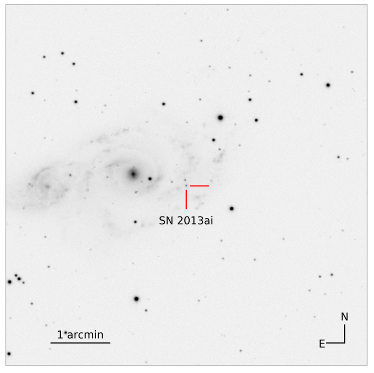
SN 2013ai was discovered at RA(2000), Dec(2000) with the Zadko 1 meter telescope at Gingin Observatory, Australia on 2013 March 1 UT at an apparent -band magnitude of 14.4 mag (Conseil et al., 2013). However, the SN was previously detected in pre-discovery images as early as 2013 February 26 UT and not detected in images taken on 2013 February 21 UT, with a limiting magnitude of from the Panoramic Survey Telescope and Rapid Response System (Pan-STARRS; Chambers et al., 2016). Thus an explosion date of 2013 February 24 UT (56347 MJD) days is adopted for the remainder of this work. The error listed on explosion date is a flat distribution without any obvious bias toward last non-detection or discovery.
The host of SN 2013ai, NGC 2207, is in the process of colliding with another galaxy, IC 2163, which makes any distance measurement based on galaxian properties uncertain. The host is a luminous infrared galaxy with a high star formation rate that produces SNe frequently, e.g. SNe 1975A, 1999ec, 2003H, 2018lab, and AT 2019eez (Kirshner et al., 1976; Jha et al., 1999; Graham et al., 2003; Sand et al., 2018; Stanek, 2019). At a redshift of 0.009, NGC 2207 is too close for a reliable redshift distance as it is not in the Hubble flow.
NGC 2207 was host to SN 1975A, a SN Ia that provides the only redshift-independent distance measurement to the galaxy. Using the GELATO classification tool (Harutyunyan et al., 2008), the best match of the 1975 January 20 spectrum of SN 1975A published by Kirshner et al. (1976) was found to be SN2003du, which had a -band decline rate of (Blondin et al., 2012). Pseudo equivalent width (pEW) measurements of the Si ii 5972 and 6355 lines from this spectrum place SN 1975A in the middle of core-normal SNe in the Branch diagram (Branch et al., 2006, 2009). In addition, the pEW of the λ5972 line is consistent with 1.1 (see Figure 17b of Folatelli et al. 2013). Following the procedures of Riess et al. (1998), and using the reproduced photometry from Kirshner et al. (1976), the SN 1975A light curves were analyzed using SNooPy (Burns et al., 2011) to estimate a distance. Fixing the B-band decline rate in the range (B) yielded a 0.1 mag difference in the distance moduli and a fit error of 0.15 mag from SNooPy. This procedure gives a final distance modulus of for NGC 2207, which we adopt in this paper.
SN 2013ai was classified as a SN II by the Public ESO Spectroscopic Survey of Transient Objects (PESSTO) (Smartt et al., 2015) due to broad H emission in its optical spectrum (Klotz et al., 2013). Archival HST-WFPC2 images are available of the field, obtained using the F336W, F439W, F555W, and F814W filters, which contained the site of SN 2013ai on 1996 May 25 UT. However, no clear single progenitor could be detected (Milisavljevic et al., 2013). These data are reanalyzed in Section 6.
Optical photometric follow up commenced soon after SN 2013ai was discovered, using ESO + EFOSC2, the 1.3 m SMARTS telescope111Operated by the SMARTS Consortium. + ANDICAM, and the 1m Swope telescope + SITe3. Swope + SITe3 images were taken as a part of the Carnegie Supernova Project II (CSP-II) (Phillips et al., 2019; Hsiao et al., 2019). In the NIR, imaging was obtained with NTT + SOFI and the 2.5 m du Pont telescope + RetroCam. A Swope -band image taken at days past explosion is shown in Figure 1.
ANDICAM data were reduced with the dedicated pipeline which subtracts the overscan and bias from each image, followed by flat fielding correction using dome flats. For EFOSC2 data, the reduction was performed using the PESSTO pipeline, as described in Smartt et al. (2015), which trims, debiases, and flat-fields images (using twilight sky flats). In addition, a fringe frame is used to correct the I-band data. The SN magnitude in each frame was measured via Point Spread Function (PSF) fitting photometry using the SNOoPy package222SNOoPy is a package for SN photometry using PSF fitting and/or template subtraction developed by E. Cappellaro. A package description can be found at https://sngroup.oapd.inaf.it/snoopy.html, with errors estimated from artificial star tests. The photometric zero point for each image was determined from aperture photometry of local sequence stars, which in turn were calibrated to Landolt fields (Landolt, 1992) observed on multiple photometric nights. Color terms were applied to the EFOCS2 and ANDICAM magnitudes using the values listed in Smartt et al. (2013) for the former and values listed on the SMARTS consortium webpages for the latter. The reduction of Swope photometry was performed as described in Phillips et al. (2019). Swope PSF photometry was performed in the same process described for ANDICAM and EFOSC2 data with standard fields observed on the same nights as the SN observations when possible. The Swope data have been converted to the standard system using the process outlined in Phillips et al. (2019). The light curves are presented without template subtraction as the SN is well separated from the host. A log of the optical photometry is given in Table 1.
| MJD | UT Date | Phase | () | () | () | () | () | () | Instrument |
|---|---|---|---|---|---|---|---|---|---|
| 56344.33 | 2013/02/21 | 2.7 | - | - | - | - | 20.7 | - | GPC1 |
| 56349.66 | 2013/02/26 | 2.7 | - | - | - | - | 18.3 | - | TAROT |
| 56351.66 | 2013/02/28 | 4.7 | - | - | - | - | 17.6 | - | TAROT |
| 56352.66 | 2013/03/01 | 5.7 | - | - | - | - | 17.4 | - | TAROT |
| 56354.05 | 2013/03/03 | 7.1 | - | - | - | - | 17.23(03) | - | EFOSC2 |
| 56354.25 | 2013/03/03 | 7.2 | 18.43(04) | 18.15(02) | 17.68(02) | 17.80(02) | 17.42(02) | 17.17(02) | SITe3 |
| 56355.08 | 2013/03/04 | 8.1 | 18.22(03) | 18.07(02) | 17.58(02) | 17.80(02) | 17.27(03) | 17.06(02) | SITe3 |
| 56356.09 | 2013/03/05 | 9.1 | - | 18.22(02) | 17.49(02) | - | 16.94(03) | 16.35(04) | ANDICAM |
| 56357.08 | 2013/03/06 | 10.1 | - | 18.09(01) | 17.45(02) | - | 16.83(01) | 16.21(02) | ANDICAM |
| 56362.15 | 2013/03/11 | 15.2 | - | 18.09(03) | 17.30(02) | - | 16.69(03) | 16.06(03) | ANDICAM |
| 56362.15 | 2013/03/11 | 15.2 | - | - | 17.34(04) | - | - | - | EFOSC2 |
| 56364.15 | 2013/03/13 | 17.2 | - | 18.14(03) | 17.29(02) | - | 16.70(03) | 16.05(03) | ANDICAM |
| 56364.15 | 2013/03/13 | 17.2 | - | - | 17.36(03) | - | - | - | EFOSC2 |
| 56368.12 | 2013/03/17 | 21.1 | - | 18.21(02) | 17.36(02) | - | 16.65(02) | 15.98(02) | ANDICAM |
| 56368.08 | 2013/03/17 | 21.1 | - | - | 17.37(03) | - | - | - | EFOSC2 |
| 56371.13 | 2013/03/20 | 24.1 | - | 18.33(03) | 17.34(04) | - | 16.60(01) | 15.93(04) | ANDICAM |
| 56373.14 | 2013/03/22 | 26.1 | - | 18.36(07) | 17.40(04) | - | 16.59(02) | 15.86(02) | ANDICAM |
| 56374.10 | 2013/03/23 | 27.1 | - | 18.46(04) | 17.40(04) | - | 16.54(04) | 15.96(03) | ANDICAM |
| 56378.05 | 2013/03/27 | 31.1 | - | 18.73(06) | 17.47(04) | - | 16.64(02) | 15.95(03) | ANDICAM |
| 56380.12 | 2013/03/29 | 33.1 | - | 18.73(08) | 17.54(04) | - | 16.69(03) | 16.02(03) | ANDICAM |
| 56385.03 | 2013/04/03 | 38.0 | - | - | 17.75(10) | - | - | - | EFOSC2 |
| 56388.07 | 2013/04/06 | 41.1 | - | 19.12(04) | 17.68(03) | - | 16.73(04) | 16.07(02) | ANDICAM |
| 56391.07 | 2013/04/09 | 44.1 | - | 19.25(05) | 17.71(03) | - | 16.79(02) | 16.02(02) | ANDICAM |
| 56394.06 | 2013/04/12 | 47.1 | - | 19.20(42) | 17.81(06) | - | 16.82(04) | 16.06(03) | ANDICAM |
| 56395.00 | 2013/04/13 | 48.0 | - | - | 17.91(03) | - | - | - | EFOSC2 |
| 56397.05 | 2013/04/15 | 50.1 | - | 19.54(08) | 17.80(03) | - | 16.82(03) | 16.17(03) | ANDICAM |
| 56400.06 | 2013/04/18 | 53.1 | - | 19.47(36) | 17.92(05) | - | 16.87(06) | 16.09(04) | ANDICAM |
| 56402.02 | 2013/04/20 | 55.0 | - | - | 18.00(04) | - | - | - | EFOSC2 |
| 56403.03 | 2013/04/21 | 56.0 | - | 19.57(09) | 17.98(05) | - | 17.02(03) | 16.19(02) | ANDICAM |
| 56411.08 | 2013/04/29 | 64.1 | - | 19.60(60) | - | - | 17.10(03) | - | EFOSC2 |
| 56414.51 | 2013/05/02 | 67.5 | - | 19.66(62) | 18.16(17) | - | 17.08(03) | 16.37(03) | ANDICAM |
| 56680.17 | 2014/01/23 | 333.2 | - | - | - | - | - | 21.57(22) | EFOSC2 |
| 56695.16 | 2014/02/07 | 348.2 | - | - | 23.75(63) | - | - | 22.33(41) | EFOSC2 |
| 56708.15 | 2014/02/20 | 361.2 | - | - | 23.21(31) | - | - | - | EFOSC2 |
| 56726.09 | 2014/03/10 | 379.1 | - | - | - | - | - | 21.48(28) | EFOSC2 |
Note. — The MJD column lists the Modified Julian Date of each observation. Phase is listed in days since explosion.
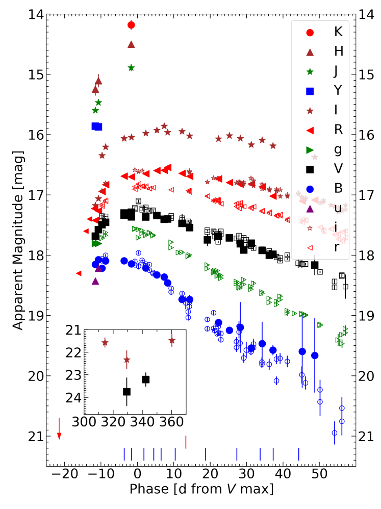
The NIR light curves from Dupont + RetroCam were reduced in the standard manner following Phillips et al. (2019). The NIR NTT + SOFI data were corrected for crosstalk, flat-fielded (using dome flats), and scattered light, performed within the PESSTO pipeline. Separate off-target sky frames were taken as part of the sequence of observations, and these were used to subtract the sky background from the on-target images. The multiple exposures taken in each filter were combined to produce a deep image on which photometry was performed. The log of NIR photometry is given in Table 2. The photometry of SN 2013ai previously published by Valenti et al. (2016) is also included. The light curves in each band, during the photospheric phase, are presented in Figure 2.
| MJD | UT Date | Phase | () | () | () | () | Instrument |
|---|---|---|---|---|---|---|---|
| 56354.25 | 2013/03/03 | 7.1 | 15.86(01) | 15.60(01) | 15.24(11) | - | RetroCam |
| 56355.08 | 2013/03/04 | 8.1 | 15.87(01) | 15.47(01) | 15.11(11) | - | RetroCam |
| 56364.10 | 2013/03/13 | 17.1 | - | 14.89(06) | 14.50(03) | 14.18(08) | SOFI |
Note. — The MJD column lists the Modified Julian Date of each observation. Phase is given in days since explosion.
Through the PESSTO collaboration, an optical spectroscopic time-series was obtained with EFOSC2 on the ESO-NTT (Buzzoni et al., 1984). Complementary, spectra were taken with the Wide-Field Spectrograph (WiFeS; Dopita et al., 2010) on the Australian National University (ANU) 2.3m Telescope as part of the ANU WiFeS Supernova Programme (Childress et al., 2016). The EFOSC2 spectra were reduced, extracted, and calibrated with the PESSTO pipeline using standard techniques (Smartt et al., 2015). All spectra were bias-subtracted and divided by a normalized lamp flat. For the Gr#16 EFOSC2 spectra, flat fields were taken immediately after the spectrum, and at the same position on the sky, to allow for the removal of the strong fringing seen at longer wavelengths. Wavelength calibration was performed with respect to an HeAr arc lamp. After extracting each spectrum the wavelength of the strong night sky emission lines were checked, and if necessary, a linear shift was applied to the dispersion solution. The spectra were flux calibrated using a sensitivity curve constructed from observations of spectrophotometric standard stars, and then telluric absorptions were removed using a scaled synthetic model of atmospheric transmission (Patat et al., 2011). The WiFeS spectra were reduced using the PyWiFeS software (Childress et al., 2013). The late time spectrum taken with Gran Telescopio Canarias (GTC) on October 30 2013 was reduced and extracted using standard IRAF (Tody, 1986) routines and was flux calibrated using a spectrophotometric standard star observed on the same night. A log of the spectroscopic observations is presented in Table 3, and the optical spectra during the photospheric phase are presented in Figure 3.
A NIR spectrum of SN 2013ai was obtained using the Folded-port Infrared Echellette (FIRE; Simcoe et al., 2013) on the Magellan Baade telescope as part CSP-II (Phillips et al., 2019; Hsiao et al., 2019). The spectrum was reduced and telluric corrected following the procedure outlined in Hsiao et al. (2019) and has been previously published in Davis et al. (2019). All observations will be made public via WISeREP (Yaron & Gal-Yam, 2012).
Further observations taken with Swift-XRT 25 days after explosion detected an X-ray source 8′′ from the SN position at a level of erg/s/cm2 (Margutti et al., 2013). Radio observations were taken using the Combined Array for Research in Millimeter-Wave Astronomy (CARMA) 10 and 11 days past explosion at 85 GHz, however, no radio source was detected at either epoch at a limit of 0.6 mJy (Zauderer et al., 2013).
| UT Date | MJD | Instrument | Phase | |
|---|---|---|---|---|
| Optical | ||||
| 2013-03-03 | 56354.1 | NTT + EFOSC2 | 7.1 | 11.3 |
| 2013-03-05 | 56356.1 | NTT + EFOSC2 | 9.1 | 9.3 |
| 2013-03-08 | 56359.5 | ANU + WiFeS | 12.0 | 5.9 |
| 2013-03-11 | 56362.2 | NTT + EFOSC2 | 15.2 | 3.2 |
| 2013-03-13 | 56364.2 | NTT + EFOSC2 | 17.2 | 1.2 |
| 2013-03-17 | 56368.1 | NTT + EFOSC2 | 21.1 | 2.7 |
| 2013-03-25 | 56376.4 | ANU + WiFeS | 29.4 | 11.0 |
| 2013-04-03 | 56385.0 | NTT + EFOSC2 | 38.0 | 19.6 |
| 2013-04-09 | 56391.4 | ANU + WiFeS | 44.4 | 26.0 |
| 2013-04-13 | 56395.0 | NTT + EFOSC2 | 48.0 | 29.6 |
| 2013-04-20 | 56402.0 | NTT + EFOSC2 | 55.0 | 36.6 |
| 2013-05-26 | 56438.3 | ANU + WiFeS | 91.3 | 72.9 |
| 2013-10-30 | 56595.5 | GTC + OSIRIS | 249.5 | 231.1 |
| NIR | ||||
| 2013-03-10 | 56361.5 | Baade + FIRE | 14.5 | 3.9 |
Note. — The MJD column lists the Modified Julian Date of each observation. Phase is given as days since explosion. Time relative to maximum, in days, is denoted .
3 Reddening
Milky Way extinction towards SN 2013ai is taken from (Schlafly & Finkbeiner, 2011). In order to estimate the extinction of SN 2013ai the equivalent width (EW) of the Na I absorption lines at the redshift of the host galaxy NGC 2207 were measured in all available WiFeS spectra as they have the highest resolution of R. Assuming Gaussian profiles for both components, we obtain an average of Å, Å, and Å. Using equation (9) from Poznanski et al. (2012) we obtain an mag. However, according to Phillips et al. (2013) the error associated with this method can be much larger than predicted by relations derived for typical Milky Way dust and gas. As a check for consistency, we used the Balmer decrement to determine the dust extinction by computing the flux ratio of H and H lines using the same WiFes spectra. The Balmer decrement was measured using the narrow host galaxy lines in the spectrum. The obtained color excess was mag. Similar results were obtained using PESSTO low resolution spectra from which we extracted a region near the SN without subtracting the background. The Balmer decrement was measured from a flux calibrated MW extinction corrected spectrum. Errors were determined by a series of Monte Carlo realizations, assuming the uncertainty is dominated by the photometric errors and therefore flux calibration. The Balmer decrement was measured for each realization, with the error taken as the standard deviation. Finally, the diffuse interstellar band (DIB) at 5780 Å was analyzed. This band appears to be very weak or non existent in the available spectra. Thus, for this work we adopt a color excess estimate of mag from the Balmer decrement and Na ID measurements.
4 Photometric Properties
The optical light curves of SN 2013ai have been previously studied by Valenti et al. (2016) and Pessi et al. (2019). The -band light curve was characterized by Davis et al. (2019) using the parameters defined by Anderson et al. (2014a). Here we combine the public data of SN 2013ai along with a previously unpublished data set to further analyze SN 2013ai.
The new data are in agreement with previous results that positioned SN 2013ai among typical fast declining SNe II with a decline rate per 100 days, (Anderson et al., 2014a), of (historically SNe IIL, see Barbon et al., 1979); and an absolute -band maximum of mag. The only photometric difference SN 2013ai displays with respect to normal SNe II is that it presents an atypically long rise time (e.g. Valenti et al., 2016). From the Pessi et al. (2019) sample, the typical rise times of SNe II are days, days, and days in the , , and bands, respectively. For SN 2013ai, the rise times are 13.05.3 days, 18.93.7 days, and 24.44.0 days, in the , , and bands, respectively. On average the rise times of SN 2013ai are 2.4 away from the mean values calculated in Pessi et al. (2019). Note that in Pessi et al. (2019) the computed rise time average for the SN II sample is longer than for other higher cadence samples (e.g. González-Gaitán et al., 2015; Gall et al., 2015; Valenti et al., 2016; Rubin, & Gal-Yam, 2016). Rubin, & Gal-Yam (2016) studied the -band light curves of 44 SNe II and found an average rise time of 7.82.8 days with the slowest rising object, PTF12hsx, taking 16.2 days to reach maximum. SN 2013ai rises significantly more slowly than any SN in the Rubin, & Gal-Yam (2016) sample. The rise time of SN 2013ai is significantly longer than that of a typical SNe II.
Late-time photometric data may be used to estimate the 56Ni mass using the procedure of Hamuy (2003) and the bolometric correction from Bersten & Hamuy (2009). However, the scarce late-time data do not allow for a decay slope to be measured, so only a lower limit of the 56Ni mass can be given as the extent of the -ray trapping can only be estimated. For 100% trapping, we get M⊙ with the error bars including the photometry error but not the reddening and distance uncertainties. There are large uncertainties associated with this lower limit as the light curve decay is highly dependent on the amount of -ray trapping. For the case of SN 1993J (see Hoeflich et al., 1993), which is a good approximation for SN 2013ai at late times (see Section 7), 79% of -rays had escaped at 350 days past explosion. However, 56Co decays in two channels, electron capture and positron capture. Approximately 4% of the decays are positron capture and will remain trapped, giving a total trapping of %. This suggests that the 56Ni mass lower limit from observations could be underestimated by up to a factor of 4, translating to a 56Ni mass of M⊙. Similarly, assuming that the light curve is powered by 56Co decay past 50 days from explosion, i.e. constant slope, the magnitude difference of pure 56Co decay to the observed light curve gives a similar result.
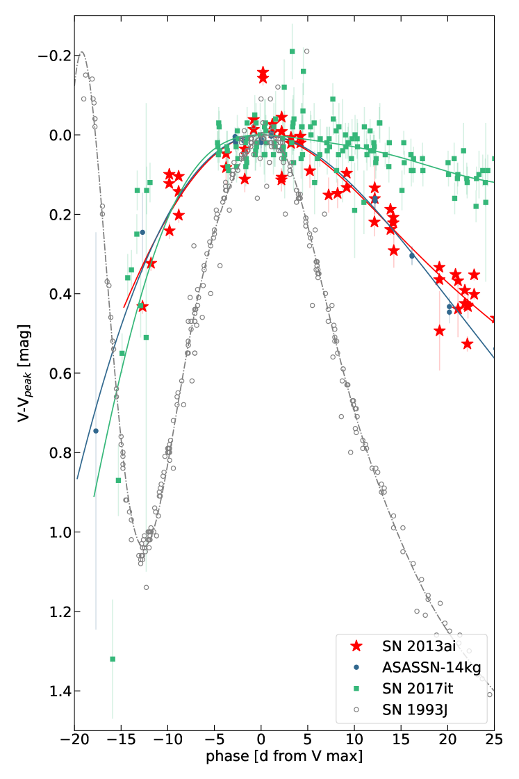
SN 2013ai may be compared with two other SNe II that were found in the literature: ASASSN-14kg (Valenti et al., 2016) and SN 2017it (Afsariardchi et al., 2019). ASASSN-14kg was chosen as it was found to have the most similar light curve to SN 2013ai. SN 2017it was published as a high 56Ni mass SN II with a long rise, so despite its slow decline post-maximum, bears comparison to SN 2013ai. Photometry from Valenti et al. (2016) shows a -band rise time for ASASSN-14kg of 18 days while Afsariardchi et al. (2019) report a -band rise time of 20 days for SN 2017it. In order to recalculate the rise times of these objects in a uniform fashion, the explosion epoch of the comparison SNe is taken as the mid point between the last non-detection and the first detection while considering the error to be half the difference between said epochs. The light curves were then interpolated via a Gaussian process method using the Python library GPy333https://sheffieldml.github.io/GPy/. Finally, the maximum date was obtained from the interpolated light curve and the rise times were calculated. Results are presented in Table 4. It can be seen in Figure 4 that the behavior of SN 2013ai around peak is similar to ASASSN-14kg. SN 2017it, despite the long rise, exhibits a post-maximum decline similar to a normal SN II. For further comparison to the SN IIb subclass, SN 1993J, is added as an example of a typical SN IIb light curve. The rise time of SN 2013ai is similar to a SN IIb, however, the post-maximum decline is much slower.
To calculate the bolometric light curve, the Milky Way and NGC 2207 dust reddening corrected photometry was first converted into AB magnitudes using the spectral energy distribution of Vega. Monochromatic fluxes for each available date were numerically integrated in wavelength, obtaining the pseudo-bolometric flux (Fpbol). For the flux (FUV), a linear extrapolation was used and integrated from the observed flux at the band to zero flux at 2000 Å (see Bersten & Hamuy, 2009; Folatelli et al., 2014, for further details). To estimate the IR flux (FIR) the spectral energy distribution was fit by a grid of temperatures and angular sizes which define a black body for each point of the grid. Using the resultant grid from each black body, a probability distribution to determine the best parameters for each epoch is calculated. Afterwards, the flux was integrated from the effective wavelength of the filter to 100,000 Å, where the flux is considered negligible.
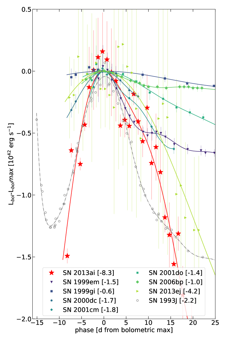
The bolometric flux was calculated as . This bolometric light curve was compared to a subsample of the bolometric light curves presented by Faran et al. (2018). Their sample includes only objects with high quality multiband data and rather good time coverage, which makes it useful for our goal of comparing SN 2013ai to a large sample of bolometric light curves computed in a uniform manner. Note that the bolometric light curves of Faran et al. (2018) were computed differently to the SN 2013ai bolometric light curves as they consider the effects in the bluer and redder wavelengths, e.g. line blanketing. However, given the uncertainties involved in calculating bolometric light curves, the comparisons presented would not significantly change if the bolometrics were recalculated. The subsample was selected such that only objects that show a clear maximum in the light curve, meaning there are data points before maximum, are considered. From the 29 objects presented in Faran et al. (2018), only 8 meet this requirement, although SN 2003hf is much more luminous than the others so it was excluded, giving 7 comparison objects. The bolometric light curve of SN 1993J (Richmond et al., 1994) is also presented for comparison. Figure 5 shows that SN 2013ai is the fastest decliner, except for the SN IIb SN 1993J. Using the explosion dates published by Faran et al. (2018) we obtain a mean bolometric rise time of the subsample of 8.62.0 days while the bolometric rise time of SN 2013ai is 14.34.1 days.
| SN | Last Non-detection | First Detection | Explosion Epoch | Reference | -band Max Epoch | -band Rise Time |
|---|---|---|---|---|---|---|
| ASASSN-14kg | 56972.4 | 56973.5 | 56972.90.5 | Nicolas et al. (2014) | 56991.12.8 | 18.12.9 |
| SN 2013ai | 56344.3 | 56349.7 | 56347.02.7 | Conseil et al. (2013) | 56365.92.6 | 18.93.7 |
| SN 2017it | 57745.5 | 57746.9 | 57746.20.7 | Afsariardchi et al. (2019) | 57762.84.2 | 16.64.3 |
Note. — All dates are given in MJD.
5 Spectral Properties
The optical and NIR spectra of SN 2013ai were analyzed quantitatively by measuring expansion velocities and pEWs for every feature present. These techniques have been implemented succesfully before to study large samples of SNe II and their diversity (e.g. Gutiérrez et al., 2017; Davis et al., 2019; de Jaeger et al., 2019).
5.1 Time Evolution
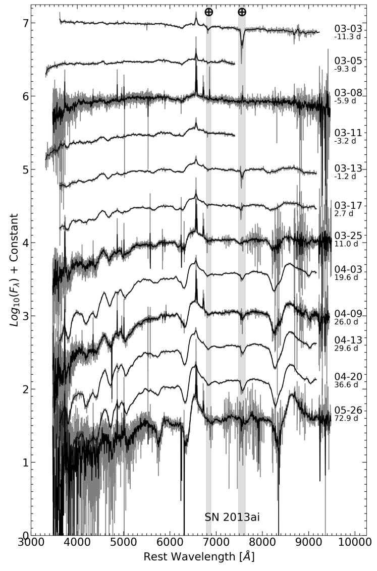
Figure 3 shows the optical spectra of SN 2013ai. In the optical, at all epochs, we see narrow optical emission in H, H, [O ii] 3727, [O iii] 5007 and [S ii] 6717, 6731 at the redshift of NGC 2207. The earliest spectra, taken days before maximum, show only a broad H P Cygni profile with narrow Na I D 5890 and 5896 likely from the interstellar medium (ISM). H is not present until later times, first seen around days before maximum. A montage of the optical spectra is presented in Figure 3.
Starting with the spectrum taken days after maximum, the H absorption becomes split, likely due to Si ii 6355 at these early times (Gutiérrez et al., 2017). Fe-group lines are also present during this epoch, primarily Fe ii 5169, 5267, and 5363. We also see the emergence of the Ca ii NIR triplet as a broad and blended P Cygni line around 8500 Å.
From days after maximum, SN 2013ai became even redder, as more flux is lost to absorption by Cr, Sc, Ba and Fe in the blue. The usual Fe-group lines seen in SNe II are present between 3500-5500 Å; however, these lines are weaker than what are seen in a normal SN II (see Gutiérrez et al. 2017; de Jaeger et al. 2019). H has a strong absorption component in its P Cygni profile, with a minimum at a velocity of 11,000 km s-1, while the second absorption, which was tentatively associated with Si ii, is still present as a “notch” in the feature. There is a lack of absorption from Sc ii and Ba ii on the blue side of the H absorption line.
By days after maximum, the notch in H is no longer present in the spectrum of SN 2013ai, suggesting that the notch was not due to high velocity (HV) H i (see Gutiérrez et al. 2017 for more information on this feature). The spectrum shows relatively little evolution over the following period, from to days post explosion, the continuum continues to become redder, while the most notable change in the lines is an increase in the strength of the Na I D absorption.
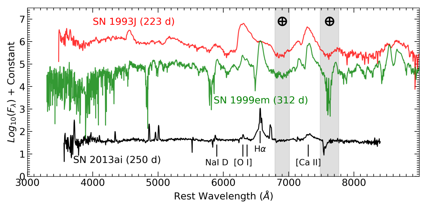
The late time optical spectrum obtained days after maximum with GTC+OSIRIS is shown in Figure 6. This spectrum was taken 250 days from the estimated explosion epoch and is shown in comparison to the SN IIP SNe 1999em and the SN IIb SN 1993J at similar times. The spectrum of SN 2013ai contains very little flux from the SN. Nonetheless, several lines characteristic of core-collapse SNe in their nebular phase are detected, namely broad H emission, [Ca ii] 7291, and possibly [O i] 6300. The reddening corrected [Ca ii] to [O i] line ratio appears approximately similar to that in SN 2004et (see Jerkstrand et al., 2012), suggesting that the core mass of the star which exploded was probably quite similar and not exceptionally massive. However, the weakness of these lines makes it difficult to accurately measure a flux ratio and suggest that the SN is not sufficiently nebular for an accurate progenitor to be assumed using the method of Jerkstrand et al. (2012). The H profile at this epoch is dominated by emission and shows a profile with a wide base and narrow top with no absorption. Together with the early X-ray observations, as noted in Section 2, this suggests interaction with circumstellar material (CSM).
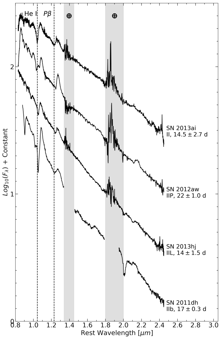
The NIR spectrum of SN 2013ai is shown in Figure 7 and exhibits mostly hydrogen and helium features, such as and and the He i/ blend. In the NIR, SN 2013ai does not exhibit any lack of features like the absence Sc ii and Ba ii in the optical.
5.2 Comparison to Other Core-Collapse SNe
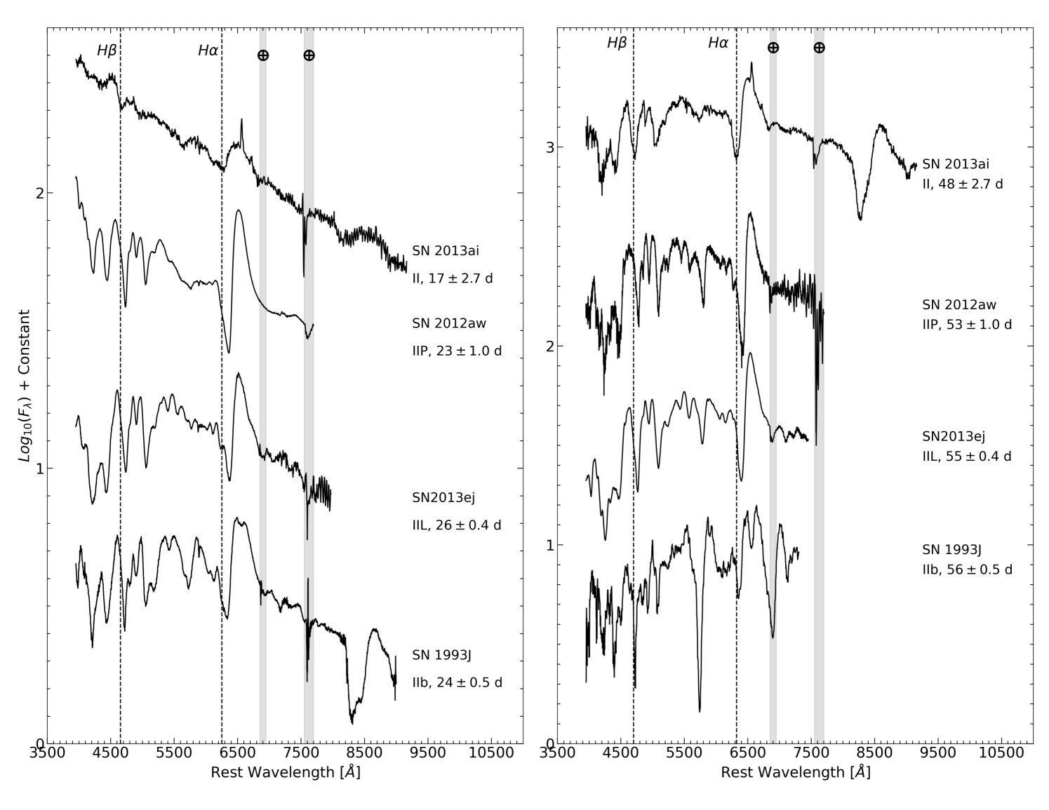
Figure 8 shows optical spectra of SN 2013ai compared to other SNe at similar phases. Included are examples of well-studied SNe IIP, IIL, and IIb. This comparison highlights the uniqueness of SN 2013ai in the features seen, their strengths, and expansion velocities. As previously noted, there is a lack of features on the blue side of H and the Na/He absorption around 5990 Å is significantly shallower than that seen in a normal SN II/IIb.
Figure 7 shows the 14.5 day NIR spectrum of SN 2013ai compared to other SNe II at similar epochs. The SN does not show any signs of being a NIR weak SN II (Davis et al., 2019); however, at such early times it is not always possible to determine a NIR spectroscopic subclass. The He i line is stronger than that of SN 2013hj at a similar phase. Both SNe show a boxy emission profile. Overall, the NIR features of SN 2013ai are much more normal than in the optical. However, similar to the optical, the features in the NIR have much higher velocities than other SNe IIP/L at similar times.
The top row of Figure 9 compares the pEW of all optical features present in the spectra of SN 2013ai with the mean from Gutiérrez et al. (2017) and all data from the de Jaeger et al. (2019) and Liu et al. (2016) samples. The metal lines, from 4500-5500 Å, of SN 2013ai evolve like those of a typical SN II. The 5990 Å He/Na blend is particularly interesting due to its weakness at later times. The pEWs of all features seen in the optical lie amongst normal SNe II values. Similarly, the top row of Figure 10 compares the pEW of all NIR spectral features of SN 2013ai with the sample from Davis et al. (2019). The NIR pEWs, like the optical, lie within the large comparative samples.
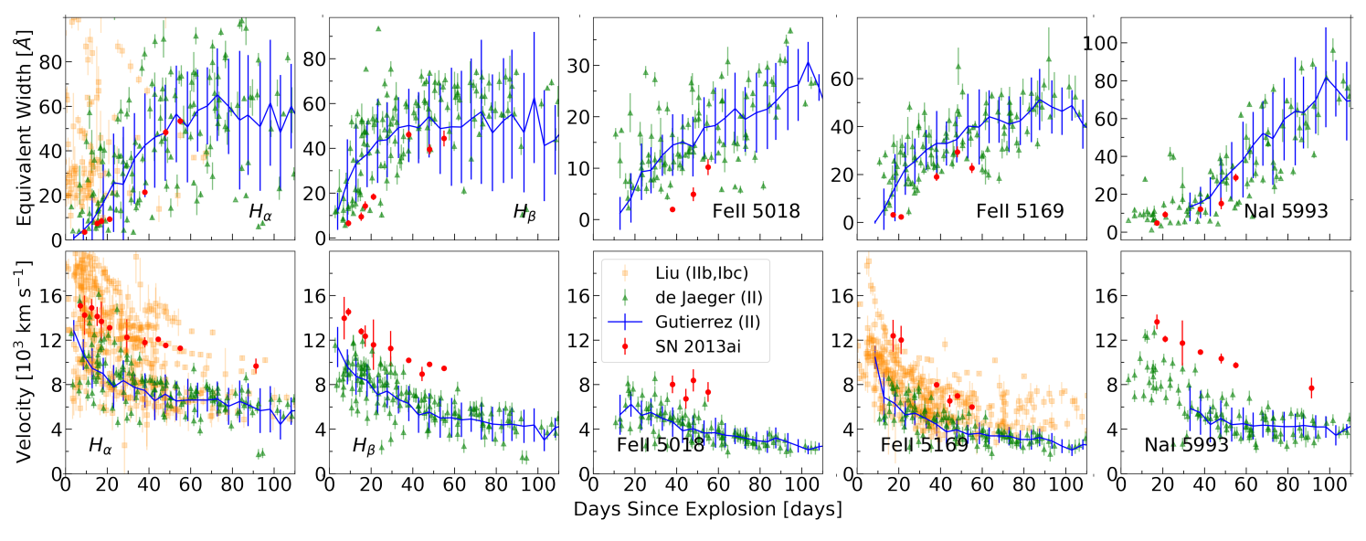
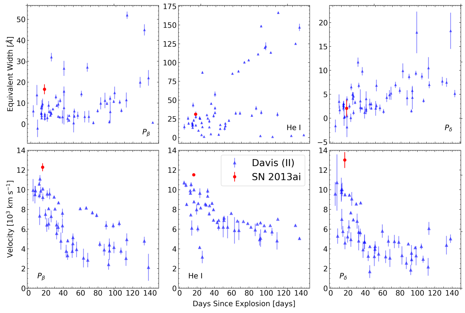
The bottom row of Figure 9 shows the absorption velocities of SN 2013ai compared to the samples of Liu et al. (2016), Gutiérrez et al. (2017), and de Jaeger et al. (2019). SN 2013ai exhibits high velocities in all features observed, for a SN II. The 5990 Å He/Na blend is particularly interesting due to its high velocities if assumed to be Na i , giving velocities over 13,000 km s-1 at early times. While the Fe ii velocities are closer to normal SN II values, they are still noticeably higher than the comparative SN II samples, with the velocities more similar to SESNe. Despite the high velocities, the evolution is decreasing with time, as that of a normal SN II. Figure 10 shows the NIR absorption velocities of SN 2013ai compared to that of the data from Davis et al. (2019). Much like the optical, the velocities are significantly higher than the sample, , with the P and P features around 12,000-13,000 km s-1 and He i around 11,500 km s-1at 22 days past maximum. The offset of velocities from typical SN II values are similar in the optical and NIR. The normal pEWs and high velocities of SN 2013ai suggest that the features are not broad, but are fast, like those of a SN IIb. However, the spectral features present are typical of a SN II.
The optical absorption velocities at 50 days past explosion, the middle of the plateau for a normal SN II, were also compared to the Gutiérrez et al. (2017) and de Jaeger et al. (2019) samples in order to see if any other SNe II have been found with velocities as high as SN 2013ai. No SNe with velocities as high as SN 2013ai were found, except for SN 2007ld from the Gutiérrez et al. (2017) sample, which has a 50 day H velocity over 11,000 km s-1. SN 2007ld has a normal photometric and spectroscopic evolution; however, it shows some contamination in the H emission profile which could be due to He i, a common sign of a SN IIb. Unfortunately, SN 2007ld has no spectra towards the end of its plateau, when a SN IIb can be easily identified. SN 2007ld does not exhibit a long rising light curve or a quick decline after maximum. Super-luminous SNe (e.g. SN 2013fc, SN 2016gsd Kangas et al., 2016; Reynolds et al., 2020) are not included for comparison as SN 2013ai is not super-luminous. However, see SN 2016gsd (Reynolds et al., 2020) for a super-luminous SNe II that exhibits high velocities similar to SN 2013ai.
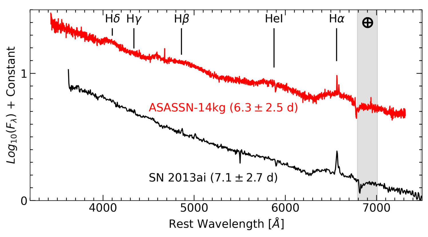
The spectra of SNe with similar rise times to SN 2013ai (see Section 4) were also examined. The classification spectrum of ASASSN-14kg is plotted with the earliest spectrum of SN 2013ai in Figure 11. The spectra look similar at these early times. There are no later spectra taken of ASASSN-14kg. ASASSN-14kg has a well defined explosion date, MJD (Nicolas et al., 2014). Given the similarity of the light curves and early spectra of ASASSN-14g and SN 2013ai, it is likely that SN 2013ai is around the same phase from explosion in the spectra seen in Figure 11. Afsariardchi et al. (2019) presented the H velocity of SN 2017it at 93 days past explosion, which is higher than that of a normal SNe II. However, it is still 1000 km s-1 slower than SN 2013ai. We were unable to find any SN II with expansion velocities comparable to SN 2013ai during the photospheric phase. However, the similarity of the early-time spectra and light curves of ASASSN-14kg and SN 2013ai suggests that they could be alike.
6 Progenitor
6.1 Pre-explosion Observations
Pre-explosion HST observations were available for SN 2013ai, consisting of HST+Wide-Field and Planetary Camera 2 (WFPC2) images taken on 1996 May 25, see Figure 12. The SN location lies on the WF2 chip, which has a pixel scale of 0.1″/pixel. Four exposures, consisting of two cr-split pairs, were taken in each of the F336W, F439W, F555W, and F814W filters, with total exposure times of 2000s, 2000s, 660s, and 720s, respectively. The pipeline reduced _c0f files were downloaded from the Mikulski Archive for Space Telescopes (MAST)444http://archive.stsci.edu/. The images were first masked with their associated _c1f files, and the cr-split pairs were combined to reject cosmic rays using the crmask task within IRAF. Finally, the dithered images in each filter were aligned and coadded.
Unfortunately, the SN position lies very close to the charge transfer trap 2-337 on the WF2 chip in all images (Whitmore & Wiggs, 1995), which gives rise to a bad column artefact. While it is possible to attempt to reconstruct the flux lost due to the trap, as dithered exposures were available, we instead ensured that the bad column was masked in both cr-split pairs for each filter before coadding. As the cr-split pairs in each filter were offset by 3 pixels in the x direction, the defect (when masked) does not contribute to the final image when they are shifted and combined.
We also attempted to use the drizzle algorithm (Fruchter & Hook, 1997) as implemented in astrodrizzle within the drizzlepac package to improve the spatial resolution of the F814W image. Before drizzling, the bad column close to the position of SN 2013ai was flagged in the data quality image. A series of drizzled images were produced, to test the effect of varying the output pixel scale and the size of the drop. However, in all cases a faint artefact was still visible at the position of SN 2013ai in the final image. It is likely that the artefact in the output image results from the interpolation over the masked bad column. Thus the drizzled images were not considered any further.
To identify the position of SN 2013ai in our pre-explosion images, we obtained Ks filter imaging of SN 2013ai with the Nasmyth Adaptive Optics System and Near-Infrared Imager and Spectrograph (NAOS-CONICA; NaCo) on the Very Large Telescope UT4 over 2013 March 3-4. SN 2013ai itself was used as a guide star for NAOS, while the S54 camera was employed on CONICA, yielding a pixel scale of 0.0543″/ pixel, over a field of view of 56″56″. Daytime calibration data consisting of flat fields and long and short exposure darks were reduced with the NaCo pipeline (version 4.3.1), to give a master flat field and a map of aberrant pixels on the detector. Using these, the individual science frames were masked and flat-fielded. All images of SN 2013ai were dithered on-source, facilitating the subtraction of the sky background using the IRAF xdimsum package. After sky-subtraction, the individual frames were aligned and combined to yield a single, deep image with a total exposure time of 5040s.
The NaCo post-explosion image was aligned to the pre-explosion WFPC2 F814W image using a geometric transformation derived from the pixel coordinates of sources common to both images. Two separate sets of sources were used for the alignment: a “good” set of 21 sources which were clearly point-like, detected with good S/N, and which appear to lie within NGC 2207, and a larger superset of 31 sources which we term the “complete” set, where the signal to noise (S/N) of sources were lower, and which also included foreground and slightly extended objects. For both the “good” and “complete” sets, the pixel coordinates of each source were measured in the WFPC2 and NaCo frames, and three separate geometric transformations were then derived using the lists of matched coordinates, one allowing for translation, rotation, and scaling in x and y, and two which also included second and third order polynomial terms, respectively.
The pixel coordinates of SN 2013ai were measured in the NaCo image using three different algorithms (centroid, gauss and ofilter within IRAF), which had a standard deviation of only 0.05 pixels, or 3 mas. The average of the three algorithms was taken as the position of SN 2013ai in the NaCo image. This position was then transformed to the pixel coordinates of the pre-explosion image using each of the transformations derived using both the “good” and “complete” sources. The standard deviation of the transformed positions was 16 mas, and we take this to be indicative of the uncertainty in SN position depending on the geometry or sources used for the alignment. We add this in quadrature with the uncertainty in the SN position in the NaCo observation (3 mas), and the average of the RMS error found when fitting each transformation (58 mas), to obtain the total uncertainty of 60 mas on the location of SN 2013ai in the WFPC2 image.
6.2 Progenitor Age Estimate
The SN falls close to, but is not coincident, with a source in the WFPC2 image, which we designate “Source A”. The centre of Source A (see Fig. 12), as measured using three centering algorithms within IRAF phot, lies 193 mas (1.93 pixels) from the transformed SN position. This offset is a factor 3 greater than the uncertainty in the transformed position of SN 2013ai (60 mas) and so we discount the possibility that this is a single stellar progenitor of SN 2013ai.
By eye, Source A appears to be somewhat extended. To test this, 14 isolated, point-like sources were fit with Moffat profiles to determine their full-width at half maximum (FWHM). The average FWHM of these sources was 1.60.2 pixels. Source A is significantly broader, with a FWHM of 2.5 pixels. On these grounds, it appears that the source may be an unresolved cluster or complex (2.5 WF pixels corresponds to a physical scale of 46 pc at the distance of NGC 2207).
While the position of SN 2013ai lies outside the FWHM of Source A, it still appears to fall within the wings of the PSF. To quantify the degree to which SN 2013ai lies within the position of Source A, the latter was fit with a Moffat profile. Then, we integrated under this profile to determine the flux within an aperture with a radius corresponding to the distance from Source A to SN 2013ai. Assuming that SN 2013ai is associated with a cluster, it was found that 97 percent of the flux of Source A is in the position of SN 2013ai. In the remainder of this section, we consider the implications for the progenitor of SN 2013ai both if it was associated with Source A, and if it was unrelated.
Photometry was performed on Source A using hstphot, (Dolphin, 2000a) a stand-alone photometry package for use with WFPC2 data. hstphot includes corrections for charge transfer efficiency (CTE) losses, aperture corrections, and zeropoints appropriate to WFPC2 (Dolphin, 2000b). While Source A is somewhat broader than most point sources in the field, it is still relatively well fit by a PSF. We measure PSF-fitted magnitudes for Source A in the HST flight system (Holtzman et al., 1995), with updated zeropoints as per Andrew Dolphin’s webpages555http://americano.dolphinsim.com/wfpc2_calib/ of F336W=22.680.12 mag, F439W=23.900.15 mag, F555W=23.400.12 mag, F814W=22.600.13 mag. Transforming to the standard UBVRI system, these correspond to U=22.680.12 mag, B=23.890.15 mag, V=23.380.12 mag, I=22.560.13 mag. As a test of the PSF-fitting results, aperture photometry was also performed using a small (2 WF pixel) aperture. For all four filters, the difference between PSF-fitting and aperture photometry was 0.1 mag, i.e. less than the photometric error.
To estimate an age for Source A, the chorizos SED-fitting package was used (Maíz-Apellániz, 2004). A grid of Starburst99 models was fit (Leitherer et al., 1999) to the measured WFPC2 photometry of the source, constraining the reddening-law parameter R5495 to be 3.1, and the metallicity to the solar value, while allowing the cluster age and extinction to vary. The results of the fitting procedure are shown in Figure 13. The best fitting model (shown in the left panel) has an age of 7.9 Myr and a relatively low extinction of E(4405-5495)=0.12 mag. Comparing to the STARS models666https://people.ast.cam.ac.uk/ stars/ (Eggleton et al., 2011), such a cluster age would imply a progenitor mass of 21 M⊙; however, we note that there are also reasonable fits for 11.2 Myr, giving a lower progenitor mass of 17 M⊙ and higher extinction. The low mass best fit of M⊙ is at the high end of SN II progenitor masses (Smartt et al., 2009; Sukhbold & Adams, 2020).
The extinction towards the cluster inferred by the fit is considerably lower than that seen towards SN 2013ai itself. There is a tail of solutions in the plane which accommodates a reddening of E(4405-5495)=0.7 mag, which is consistent with that seen towards the SN. However, these solutions require the cluster to be younger than 3 Myr, which would in turn lead to a progenitor which is extremely massive, and probably inconsistent with the maximum mass of a star that can maintain its H envelope to the point of core-collapse.
Further analysis was done using the Bayesian fitting technique of Maund (2018), which addresses cluster mass, distances, and filter transformations. Both the WFPC2 photometry and WFPC2 photometry converted to Johnson-Cousins photometry were included as seperate runs. Given the luminosity of the cluster, the mass is constrained to lie in the range . At such masses, individual, luminous stars may have a disproportionate influence on the colour of the cluster that might cause deviations from the expected colour-sequence predicted by STARBURST99 (for much more massive clusters of ).
The progenitor of SN 2013ai could be a single, isolated red supergiant as found for other Type II SNe. The relatively bright cluster nearby makes the identification of such a progenitor difficult, as the flux in the wings of the cluster may mask that of a fainter progenitor close by. The most convincing demonstration of such a progenitor would rely on image subtraction, where a flux deficit in new HST images taken after SN 2013ai has faded would indicate the absence of progenitor flux which was present in pre-explosion images. As demonstrated by Maund et al. (2014) and Folatelli et al. (2015), difference imaging using late-time data can substantially improve the precision and sensitivity of limits placed on SN progenitors. While such a test will have to wait for new observational data, it is still possible to estimate the sensitivity of pre-explosion data to a single red supergiant progenitor. From photometry of point sources close to the SN position, we estimate a limiting magnitude of F814W 24.5 mag for the WFPC2 images. At the distance of NGC 2207, this would imply an absolute magnitude for the progenitor of F814W-9 mag, which unfortunately only allows us to constrain the luminosity of the progenitor to log L/L⊙5.5. For single star models, this luminosity corresponds to a progenitor zero age main sequence mass of 24 M⊙ (Eldridge & Tout, 2004).
7 Modeling
7.1 Modeling Background
Determining the properties of CCSNe poses a challenge due to the wide range of parameters, e.g. progenitor mass, mass loss pre-explosion, explosion mechanism, mixing, and possible interaction, which affect the observational features. However, using a combination of empirical measurements and modeling we attempt to reconstruct these properties for SN 2013ai and motivate the use of a SN 1993J inspired model.
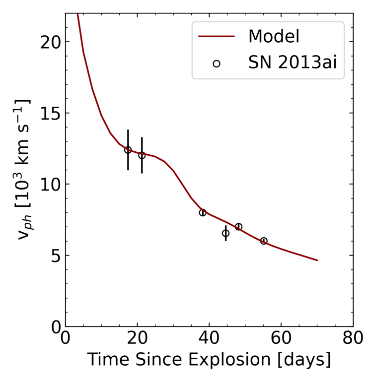
The chemical and density structures of the outer layers of the progenitor are revealed by the spectral evolution. In general, at early epochs, the spectral features are formed at or above the electron scattering photosphere in the H-rich layers. During this time, the photosphere can be traced with measurements of weak lines that form near the photosphere, e.g. Fe ii. The inner edge of the H-rich layers is determined by the point in time when the Doppler shifts of the Balmer lines becomes constant, around 40 days past explosion in SN 2013ai, whereas Fe ii still receeds. At the photosphere, the ejecta density profile of a SN II can be approximated by a power law, much like that of a stellar atmosphere, , with the density slope and the radius at a point in the ejecta (Hoeflich, 1990). Before the recombination phase of H, the differential Doppler shift between Balmer series H-lines can be used to reconstruct the density structure by integration of the density and slope (see Hoeflich, 1988, 1990, for applications to SNe II). The result of applying this technique to SN 2013ai gives a density slope, n, ranging from 12-25. A typical SN II has a density slope of 10 at early times (Hoeflich, 1990), significantly flatter than that of SN 2013ai. The steep density profile, H line profiles, and Doppler shifts are more similar to SN 1993J than the other SNe compared to (see Figures 8 and 10) with both SNe having photospheric velocities of 12,500 km s-1 at the time of the transition between the H- and He-rich layers, suggesting a similar specific energy in the H-rich layers.
Around a week after maximum, Fe ii is used to trace the photosphere. This is around the same time that a sharp drop in the Fe ii velocity is observed, as seen in Figure 9. The drop in velocity is likely caused by the photosphere receding quickly through the He layers into the carbon/oxygen (C/O) core. He i has a high ionization potential and requires high energy nonthermal photons to be observed (Graham, 1988). We see little evidence of He i in the optical which supports the notion that the jump in Fe ii velocity is caused by the photosphere quickly passing through the He layer. In the NIR, He i is seen, however, this He feature is the basis for many other He transitions. Thus, even an object with little He should show NIR He i given its high population.
The light curves are powered by the energy deposition due to the propagating shock wave, the radioactive decay of , and the recombination energy. The rise time is dominated by the diffusion time scales in the optically thick inner layers, and the light curve tail is governed by radioactive decay and, possibly, interaction with the CSM and ISM. The rise time of SN 2013ai is typical of a SN IIb and in particular similar to that of the prototypical SN IIb SN 1993J, which, together with the spectroscopic similarities highlighted above, motivate us to use SN1993J as a starting point to model SN 2013ai. SN 1993J was extensively modeled by Hoeflich et al. (1993) and was found to have a layered He-C/O core of M⊙ with an outer H-rich layer mass of 3 M⊙ originating from a progenitor with a main sequence mass () of 25 M⊙. Note that the final H, He, and C/O core masses depend on the phase of stellar evolution during which mass-loss occurs.
7.2 Modeling Results
For the progenitor evolution of SN 2013ai, we use the stellar evolution code MESA (Paxton et al., 2011). To trigger the explosion, the explosion energy () is put in the inner region as a thermal bomb which causes the ejection of the envelope leaving behind a neutron star or a black hole. For computational efficiency and to cover a sufficiently wide range of parameters, we first used the code developed by Bersten et al. (2011) to model SN 2013ai. To verify and further constrain these models, we then modeled SN 2013ai with the non-LTE hydrodynamical-radiation code HYDRA (Hoeflich, 2003, 2009). A wide range of , , and mixing, including pure C/O cores, were evaluated. We will omit the “failed” attempts.
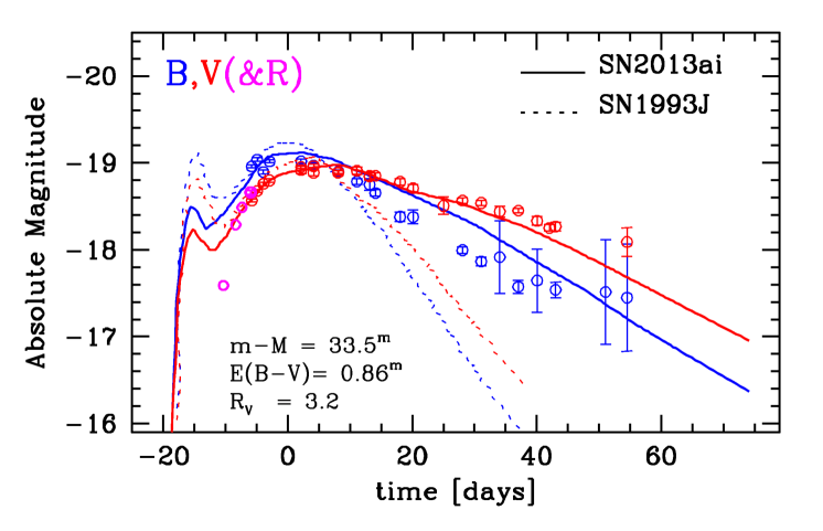
The comparison between a frequency independent model from the code of Bersten et al. (2011) with the photometry is shown in Figure 14 using depth dependent mean opacities based on SN 1993J and originating from a 20 M⊙ star. The resulting models have 0.55 M⊙ of 56Ni. Such a high 56Ni mass is problematic for the explosion of a massive star both from observations and theory (see Thielemann et al. 2018 for a review). The bolometric light curve, in principle, is a sensitive measure of the physical parameters (e.g. Suntzeff et al., 1992; Bersten et al., 2011). Despite the advantage of the bolometric light curve, three problem zones may be identified: 1) the reconstruction of the bolometric light curve, 2) distance uncertainties, and 3) asymmetries. Moreover, using the bolometric light curve reduces the information for finding model parameters. Due to these uncertainties, we use monochromatic light curves based on detailed non-LTE models.
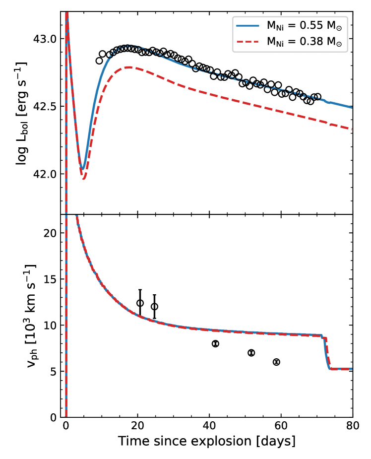
In Figures 15 and 16, we show the results of HYDRA starting with the progenitor of SN 1993J but modifying the explosion energy, the mass of the H-rich layers, the explosion energy, and the 56Ni mass. The H-rich layer mass was adjusted to 0.2 M⊙, and the 56Ni mass to 0.3 M⊙. These models are based on the results from the previously mentioned models, hereafter referred to as “LC models”. The results between best fit models of our simulations, presented as (LC, HYDRA), give consistent results within the uncertainties: M⊙, foe7771 foe = ergs, and M⊙.
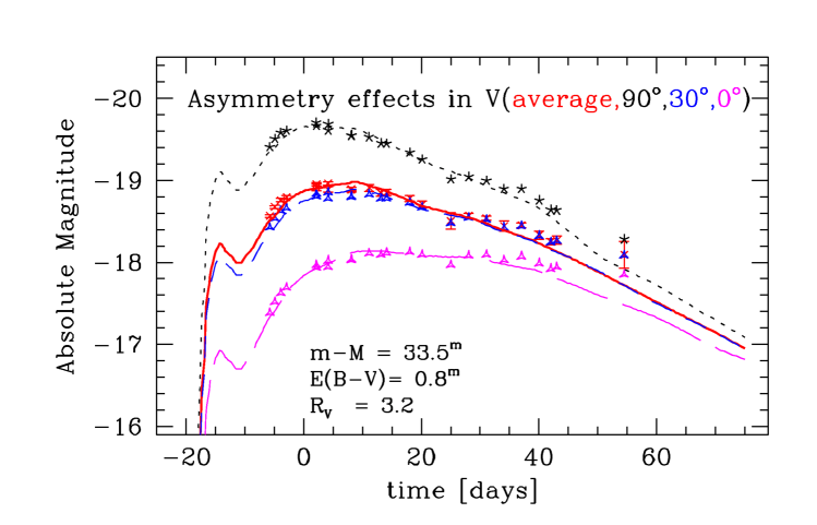
Given the model best fits, the effect of uncertainties on the , , C/O core mass, and distance modulus must be discussed. Linear polarizations give evidence for a symmetry axis and bipolar explosions with indicating axis ratios; a measure of how non-spherical an object is, of 1/2-1/4 (Wang et al., 1998; Maund et al., 2007a, b; Stevance et al., 2016; Reilly et al., 2017). To estimate the uncertainty for the light curves, we use SN 1998bw/GRB980425 as a proxy for the explosion of a massive stripped envelope SN (Hoeflich et al., 1999). Detailed analysis of polarization spectra resulted in an axis ratio of 0.7 for SN 1998bw seen from an angle of (Hoeflich, 1995) but with significant uncertainties as discussed in Stevance et al. (2020). The possible effect of asymmetry on the -band light curve of SN 2013ai is shown in Figure 17. Asymmetry may change the shape of the light curve by varying the maximum brightness up to mag, placing SN 2013ai near superluminous SNe (see Figure 17), and can shift the rise time by about 10 days.
Even for the same model, the light curve rises more slowly and shows a lower maximum brightness that directly translates into uncertainties in , and the C/O core mass. The error for the asymmetry and the shape may be regarded as an upper limit because even for purely jet-driven explosions of CCSNe, an extended outer envelope tends to become more spherical with time (Khokhlov et al., 1999; Hoeflich et al., 2004; Couch et al., 2009). The colors are found to be less sensitive as they are a measure of the physical conditions at the photosphere, namely the flux density rather than the total flux. In either case, the tail of the light curve is less effected by polarization because the luminosity becomes isotropic within mag 1-2 months after the explosion, which translates directly into an error for . For the 56Ni mass, both 0.3 and 0.55 M⊙ fit the data; however, as previously mentioned M⊙ of 56Ni is higher than expected for a massive star explosion.
Though beyond the physics included in our simulations, note that the theoretical -band light curve at 250 days is fainter by 1 mag than observed. This may indicate a significant contribution by interaction between the SN-ejecta and the ISM or a pre-explosion stellar wind. This theory would also be consistent with the multi-tiered H emission profile seen in the nebular spectrum of SN 2013ai, which indicates interaction.
8 Discussion
Given the similar early time light curve timing, expansion velocities, and density structure to SESNe, we suggest that the core of SN 2013ai is closer in physical properties to a SESNe than a normal SN II. This would give SN 2013ai a dense 10 M⊙ C/O core and little hydrogen ( M⊙ from models) in its outer layers, consistent with the quick decline post-maximum. In addition, the explosion energies of SNe 2013ai and 1993J are comparable, 2.5 foe and 2.0 foe, respectively. In this scenario, the progenitor of SN 2013ai would have most of its hydrogen envelope stripped before explosion, much like a SN IIb.
This brings us to the differences between SN 2013ai and SESNe. The first difference is seen in the shape of the early time, 2 weeks pre-maximum, light curve. SN 1993J, for example, shows an initial maximum and subsequent decline in the light curve lasting about one week (see Figure 4) that is powered by the energy deposited by the shock in the very outer layers. This structure of the SN 2013ai theoretical LC is very similar to that observed in SN 1993J but this phase has not been observed in SN 2013ai. In the SN 2013ai HYDRA models, the early peak is much less pronounced because the lower H-shell mass and the longer diffusion times with limited mixing, as predicted by Bersten et al. (2012). Secondly, the 56Ni mass is significantly larger in SN 2013ai than in SN 1993J, which could affect the lack of strong He i seen in the optical. However, in SN 2013ai, the much stronger He i line in the NIR is present and shows the presence of a He layer. To boost the optical He i lines in SN 1993J, models with 56Ni mixed into the outer layers of the ejecta were needed. This is also consistent with the rapid drop in velocity seen at about 1 week after maximum because the continuum opacity is low. Finally, SN 2013ai shows a much slower post-maximum decline rate over 30 days (0.5 mag) compared to the rapid decline in SN1993J, (2 mag). The difference can be attributed to strong 56Ni mixing in SN 1993J that results in a steeply increasing -ray escape, whereas SN 2013ai has almost full trapping. While the models based on Bersten et al. (2011) show general agreement with the observations, the strong mixing needed is not consistent with little He i seen in the optical.
From observations, SN 2013ai seems to be rather unusual but, overall, it fits well within the picture of an energetic explosion of a massive star which lost most (but not all) of its hydrogen envelope, which puts it at the edge of becoming a SN Ib or SN Ic, physically. However, using the observational classification scheme of SNe, SN 2013ai lies between a SN II and a SN IIb as its spectra are that of a SN II and its light curve more similar to SESNe. Explosions of massive stars may appear either as SNe II, IIb, Ib, or Ic depending on the details of the mass loss and the amount of mixing. The open question remains whether the mass loss in SN 2013ai is line driven or the result of a binary evolution. However, given its similarities to a SN IIb we cannot rule out that mass loss pre-explosion occurred in a binary system for SN 2013ai. As such, the current classification scheme may mask diversity and similarity as SN 2013ai has the spectra of a SN II but after analysis of spectra and light curves SN 2013ai lies between SNe II and SNe IIb.
9 Conclusions
SN 2013ai is a rare SN that exhibits a long light curve rise, sustained high expansion velocities, and a light curve decline similar to a SN IIL. Only one SN II was found to have comparable light curves and spectra, ASASSN-14kg. However, the lack of ASASSN-14kg data prevents a more detailed comparison between the two SNe. Some similarities were seen in light curve shape and expansion velocities when comparing SN 2013ai with SNe IIb. The data presented provide a link between different classes of SNe. In the current classification scheme, SN 2013ai lies between SNe II and SESNe with possible signs of interaction seen in the late-time H profile and early X-ray observations. The mass loss during the stellar evolution may be a decisive factor. However, similar data sets for a large number of SNe II are needed to better describe details of the explosion physics and to search for the diversity and address the question of the origin of this mass loss. We demonstrated the importance of the combination of optical and NIR spectra with light curves but, in lack of spectropolarimetry, we had to rely on similarity arguments and were unable to constrain some errors present in the early light curve data due to asymmetry.
References
- Afsariardchi et al. (2019) Afsariardchi, N., Moon, D.-S., Drout, M. R., et al. 2019, ApJ, 881, 22
- Aldering et al. (1994) Aldering, G., Humphreys, R. M., & Richmond, M. 1994, AJ, 107, 662
- Anderson et al. (2014a) Anderson, J. P., González-Gaitán, S., Hamuy, M., et al. 2014, ApJ, 786, 67
- Anderson et al. (2014b) Anderson, J. P., Dessart, L., Gutierrez, C. P., et al. 2014, MNRAS, 441, 671
- Arcavi et al. (2012) Arcavi, I., Gal-Yam, A., Cenko, S. B., et al. 2012, ApJ, 756, L30
- Arnett (1982) Arnett, W. D. 1982, ApJ, 254, 1
- Arnett et al. (1989) Arnett, W. D., Bahcall, J. N., Kirshner, R. P., et al. 1989, ARA&A, 27, 629
- Barbon et al. (1979) Barbon, R., Ciatti, F., & Rosino, L. 1979, A&A, 72, 287
- Barbon et al. (1995) Barbon, R., Benetti, S., Cappellaro, E., et al. 1995, A&AS, 110, 513
- Bersten & Hamuy (2009) Bersten, M. C. & Hamuy, M. 2009, ApJ, 701, 200
- Bersten et al. (2011) Bersten, M. C., Benvenuto, O., & Hamuy, M. 2011, ApJ, 729, 61
- Bersten et al. (2012) Bersten, M. C., Benvenuto, O. G., Nomoto, K., et al. 2012, ApJ, 757, 31. doi:10.1088/0004-637X/757/1/31
- Blondin et al. (2012) Blondin, S., Matheson, T., Kirshner, R. P., et al. 2012, AJ, 143, 126. doi:10.1088/0004-6256/143/5/126
- Branch et al. (2006) Branch, D., Dang, L. C., Hall, N., et al. 2006, PASP, 118, 560. doi:10.1086/502778
- Branch et al. (2009) Branch, D., Chau Dang, L., & Baron, E. 2009, PASP, 121, 238. doi:10.1086/597788
- Burns et al. (2011) Burns, C. R., Stritzinger, M., Phillips, M. M., et al. 2011, AJ, 141, 19. doi:10.1088/0004-6256/141/1/19
- Buzzoni et al. (1984) Buzzoni, B., Delabre, B., Dekker, H., et al. 1984, The Messenger, 38, 9
- Chambers et al. (2016) Chambers, K. C., Magnier, E. A., Metcalfe, N., et al. 2016, arXiv:1612.05560
- Childress et al. (2013) Childress, M. J., Vogt, F. P. A., Nielsen, J., Sharp, R. G., 2013, Ap&SS
- Childress et al. (2016) Childress, M. J., Tucker, B. E., Yuan, F., et al. 2016, PASA, 33, e055
- Clocchiatti, & Wheeler (1997) Clocchiatti, A., & Wheeler, J. C. 1997, ApJ, 491, 375
- Conseil et al. (2013) Conseil, E., Klotz, A., Coward, D., Zadko, J., & Boer, M. 2013, The Astronomer’s Telegram, 4849
- Contreras et al. (2010) Contreras, C., Hamuy, M., Phillips, M. M., et al. 2010, AJ, 139, 519
- Couch et al. (2009) Couch, S. M., Wheeler, J. C., & Milosavljević, M. 2009, ApJ, 696, 953
- Dall’Ora et al. (2014) Dall’Ora, M., Botticella, M. T., Pumo, M. L., et al. 2014, ApJ, 787, 139
- Davis et al. (2019) Davis, S., Hsiao, E. Y., Ashall, C., et al. 2019, ApJ, 887, 4
- de Jaeger et al. (2019) de Jaeger, T., Zheng, W., Stahl, B. E., et al. 2019, MNRAS, 490, 2799
- DeLaney et al. (2010) DeLaney, T., Rudnick, L., Stage, M. D., et al. 2010, ApJ, 725, 2038
- Della Valle (2016) Della Valle, M. 2016, Astronomical and Astrophysical Transactions, 29, 99
- Dessart & Audit (2018) Dessart, L., & Audit, E. 2018, A&A, 613, A5
- Dolphin (2000a) Dolphin A.E., 2000a, PASP, 112, 1383
- Dolphin (2000b) Dolphin A.E., 2000b, PASP, 112, 1397
- Dopita et al. (2010) Dopita, M., Rhee, J., Farage, C., et al. 2010, Ap&SS, 327, 245
- Drout et al. (2011) Drout, M. R., Soderberg, A. M., Gal-Yam, A., et al. 2011, ApJ, 741, 97
- Eggleton et al. (2011) Eggleton, P. P., Tout, C., Pols, O., et al. 2011, Astrophysics Source Code Library
- Eldridge & Tout (2004) Eldridge, J. J., & Tout, C. A. 2004, MNRAS, 353, 87
- Elmhamdi et al. (2003) Elmhamdi, A., Danziger, I. J., Chugai, N., et al. 2003, MNRAS, 338, 939
- Ergon et al. (2014) Ergon, M., Sollerman, J., Fraser, M., et al. 2014, A&A, 562, A17
- Faran et al. (2014) Faran, T., Poznanski, D., Filippenko, A. V., et al. 2014, MNRAS, 445, 554
- Faran et al. (2018) Faran, T., Nakar, E., & Poznanski, D. 2018, MNRAS, 473, 513
- Filippenko et al. (1993) Filippenko, A. V., Matheson, T., & Ho, L. C. 1993, ApJ, 415, L103
- Filippenko (1997) Filippenko, A. V. 1997, ARA&A, 35, 309
- Folatelli et al. (2013) Folatelli, G., Morrell, N., Phillips, M. M., et al. 2013, ApJ, 773, 53. doi:10.1088/0004-637X/773/1/53
- Folatelli et al. (2014) Folatelli, G., Bersten, M. C., Kuncarayakti, H., et al. 2014, ApJ, 792, 7
- Folatelli et al. (2015) Folatelli, G., Bersten, M. C., Kuncarayakti, H., et al. 2015, ApJ, 811, 147. doi:10.1088/0004-637X/811/2/147
- Fruchter & Hook (1997) Fruchter A.S., Hook R.N., 1997, PASP
- Fryxell et al. (1991) Fryxell, B., Mueller, E., & Arnett, D. 1991, ApJ, 367, 619
- Galbany et al. (2016) Galbany, L., Hamuy, M., Phillips, M. M., et al. 2016, AJ, 151, 33
- Gall et al. (2015) Gall, E. E. E., Polshaw, J., Kotak, R., et al. 2015, A&A, 582, A3
- González-Gaitán et al. (2015) González-Gaitán, S., Tominaga, N., Molina, J., et al. 2015, MNRAS, 451, 2212
- Graham (1988) Graham, J. R. 1988, ApJ, 335, L53
- Graham et al. (2003) Graham, J., Li, W., Puckett, T., et al. 2003, IAU Circ., 8045
- Gutiérrez et al. (2014) Gutiérrez, C. P., Anderson, J. P., Hamuy, M., et al. 2014, ApJ, 786, L15.
- Gutiérrez et al. (2017) Gutiérrez, C. P., Anderson, J. P., Hamuy, M., et al. 2017, ApJ, 850, 89
- Gutiérrez et al. (2017) Gutiérrez, C. P., Anderson, J. P., Hamuy, M., et al. 2017, ApJ, 850, 90
- Hack et al. (2012) Hack, W. J., Dencheva, N., Fruchter, A. S., et al. 2012, American Astronomical Society Meeting Abstracts #220
- Hamuy (2003) Hamuy, M. 2003, ApJ, 582, 905
- Harutyunyan et al. (2008) Harutyunyan, A. H., Pfahler, P., Pastorello, A., et al. 2008, A&A, 488, 383. doi:10.1051/0004-6361:20078859
- Hillier & Dessart (2019) Hillier, D. J. & Dessart, L. 2019, A&A, 631, A8
- Hoeflich (1988) Hoeflich, P. 1988, Proceedings of the Astronomical Society of Australia, 7, 434
- Hoeflich (1990) Höflich, P. 1990, A quantitative analysis of type II supernovae atmospheres
- Hoeflich et al. (1993) Hoflich, P., Langer, N., & Duschinger, M. 1993, A&A, 275, L29
- Hoeflich (1995) Höflich, P. 1995, ApJ, 440, 821
- Hoeflich et al. (1996) Hoeflich, P., Khokhlov, A., Wheeler, J. C., et al. 1996, ApJ, 472, L81
- Hoeflich et al. (1999) Höflich, P., Wheeler, J. C., & Wang, L. 1999, ApJ, 521, 179
- Hoeflich (2003) Höflich, P. 2003, Stellar Atmosphere Modeling, 371
- Hoeflich et al. (2004) Höflich, P., Wang, L., & Khoklov, A. 2004, Astrophysics and Space Science Library, 237
- Hoeflich (2009) Höflich, P. 2009, American Institute of Physics Conference Series, 161
- Hoeflich et al. (2017) Hoeflich, P., Hsiao, E. Y., Ashall, C., et al. 2017, ApJ, 846, 58
- Holtzman et al. (1995) Holtzman J.A., Burrows C.J., Casertano S., Hester J.J., Trauger J.T., Watson A.M., Worthey G., 1995, PASP, 107, 1065
- Hsiao et al. (2019) Hsiao, E. Y., Phillips, M. M., Marion, G. H., et al. 2019, PASP, 131, 014002
- Jerkstrand et al. (2012) Jerkstrand, A., Fransson, C., Maguire, K., et al. 2012, A&A, 546, A28
- Jha et al. (1999) Jha, S., Garnavich, P., Challis, P., et al. 1999, IAU Circ., 7269
- Kangas et al. (2016) Kangas, T., Mattila, S., Kankare, E., et al. 2016, MNRAS, 456, 323
- Khokhlov et al. (1999) Khokhlov, A. M., Höflich, P. A., Oran, E. S., et al. 1999, ApJ, 524, L107
- Kippen et al. (1998) Kippen, R. M., Briggs, M. S., Kommers, J. M., et al. 1998, ApJ, 506, L27
- Kirshner et al. (1976) Kirshner, R. P., Arp, H. C., & Dunlap, J. R. 1976, ApJ, 207, 44. doi:10.1086/154465
- Klotz et al. (2013) Klotz, A., Conseil, E., Fraser, M., et al. 2013, Central Bureau Electronic Telegrams, 3431, 1
- Krisciunas et al. (2017) Krisciunas, K., Contreras, C., Burns, C. R., et al. 2017, AJ, 154, 211
- Landolt (1992) Landolt, A. U. 1992, AJ, 104, 340
- Leitherer et al. (1999) Leitherer, C., Schaerer, D., Goldader, J. D., et al. 1999, ApJS, 123, 3
- Liu et al. (2016) Liu, Y.-Q., Modjaz, M., Bianco, F. B., et al. 2016, ApJ, 827, 90
- Maguire et al. (2010) Maguire, K., Di Carlo, E., Smartt, S. J., et al. 2010, MNRAS, 404, 981
- Maíz-Apellániz (2004) Maíz-Apellániz, J. 2004, PASP, 116, 859
- Margutti et al. (2013) Margutti, R., Soderberg, A., & Pooley, D. 2013, The Astronomer’s Telegram, 4901
- Matheson et al. (2000) Matheson, T., Filippenko, A. V., Ho, L. C., et al. 2000, AJ, 120, 1499. doi:10.1086/301519
- Maund et al. (2005) Maund, J. R., Smartt, S. J., & Danziger, I. J. 2005, MNRAS, 364, L33
- Maund et al. (2007a) Maund, J. R., Wheeler, J. C., Patat, F., et al. 2007, ApJ, 671, 1944
- Maund et al. (2007b) Maund, J. R., Wheeler, J. C., Patat, F., et al. 2007, MNRAS, 381, 201
- Maund et al. (2014) Maund, J. R., Reilly, E., & Mattila, S. 2014, MNRAS, 438, 938
- Maund (2018) Maund, J. R. 2018, MNRAS, 476, 2629. doi:10.1093/mnras/sty093
- Meikle et al. (1989) Meikle, W. P. S., Allen, D. A., Spyromilio, J., et al. 1989, MNRAS, 238, 193
- Milisavljevic et al. (2013) Milisavljevic, D., Soderberg, A., Foley, R., et al. 2013, The Astronomer’s Telegram, 4862
- Minkowski (1941) Minkowski, R. 1941, PASP, 53, 224
- Modjaz et al. (2014) Modjaz, M., Blondin, S., Kirshner, R. P., et al. 2014, AJ, 147, 99
- Moriya et al. (2016) Moriya, T. J., Pruzhinskaya, M. V., Ergon, M., et al. 2016, MNRAS, 455, 423
- Morozova et al. (2017) Morozova, V., Piro, A. L., & Valenti, S. 2017, ApJ, 838, 28
- Mueller et al. (1991) Mueller, E., Fryxell, B., & Arnett, D. 1991, A&A, 251, 505
- Nicolas et al. (2014) Nicolas, J., Holoien, T. W.-S., Stanek, K. Z., et al. 2014, The Astronomer’s Telegram 6714, 1
- Nomoto et al. (1995) Nomoto, K. I., Iwamoto, K., & Suzuki, T. 1995, Phys. Rep., 256, 173
- Patat et al. (2001) Patat, F., Cappellaro, E., Danziger, J., et al. 2001, ApJ, 555, 900
- Patat et al. (2011) Patat, F., Moehler, S., O’Brien, K., et al. 2011, A&A, 527, A91
- Paxton et al. (2011) Paxton, B., Bildsten, L., Dotter, A., et al. 2011, ApJS, 192, 3
- Pessi et al. (2019) Pessi, P. J., Folatelli, G., Anderson, J. P., et al. 2019, MNRAS, 488, 4239
- Phillips et al. (2013) Phillips, M. M., Simon, J. D., Morrell, N., et al. 2013, ApJ, 779, 38
- Phillips et al. (2019) Phillips, M. M., Contreras, C., Hsiao, E. Y., et al. 2019, PASP, 131, 014001
- Podsiadlowski et al. (1993) Podsiadlowski, P., Hsu, J. J. L., Joss, P. C., et al. 1993, Nature, 364, 509
- Podsiadlowski et al. (2004) Podsiadlowski, P., Langer, N., Poelarends, A. J. T., et al. 2004, ApJ, 612, 1044
- Popov (1993) Popov, D. V. 1993, ApJ, 414, 712
- Poznanski et al. (2012) Poznanski, D., Prochaska, J. X., & Bloom, J. S. 2012, MNRAS, 426, 1465
- Prentice, & Mazzali (2017) Prentice, S. J., & Mazzali, P. A. 2017, MNRAS, 469, 2672
- Prentice et al. (2019) Prentice, S. J., Ashall, C., James, P. A., et al. 2019, MNRAS, 485, 1559
- Pun et al. (1995) Pun, C. S. J., Kirshner, R. P., Sonneborn, G., et al. 1995, ApJS, 99, 223
- Rayner et al. (2003) Rayner, J. T., Toomey, D. W., Onaka, P. M., et al. 2003, PASP, 115, 362
- Reilly et al. (2017) Reilly, E., Maund, J. R., Baade, D., et al. 2017, MNRAS, 470, 1491
- Reynolds et al. (2020) Reynolds, T. M., Fraser, M., Mattila, S., et al. 2020, MNRAS, 493, 1761
- Richmond et al. (1994) Richmond, M. W., Treffers, R. R., Filippenko, A. V., et al. 1994, AJ, 107, 1022
- Riess et al. (1998) Riess, A. G., Nugent, P., Filippenko, A. V., et al. 1998, ApJ, 504, 935. doi:10.1086/306106
- Rubin, & Gal-Yam (2016) Rubin, A., & Gal-Yam, A. 2016, ApJ, 828, 111
- Sand et al. (2018) Sand, D. J., Valenti, S., Lundquist, M., et al. 2018, Transient Name Server Discovery Report, 2018-2000
- Sanders et al. (2015) Sanders, N. E., Soderberg, A. M., Gezari, S., et al. 2015, ApJ, 799, 208
- Schlafly & Finkbeiner (2011) Schlafly, E. F. & Finkbeiner, D. P. 2011, ApJ, 737, 103
- Shivvers et al. (2017) Shivvers, I., Modjaz, M., Zheng, W., et al. 2017, PASP, 129, 054201
- Simcoe et al. (2013) Simcoe, R. A., Burgasser, A. J., Schechter, P. L., et al. 2013, PASP, 125, 270
- Smartt et al. (2004) Smartt, S. J., Maund, J. R., Hendry, M. A., et al. 2004, Science, 303, 499
- Smartt et al. (2009) Smartt, S.J., Eldridge J.J., Crockett R.M., Maund J.R. 2009, MNRAS, 395, 1409
- Smartt et al. (2013) Smartt, S. J., Valenti, S., Fraser, M., et al. 2013, The Messenger, 154, 50
- Smartt et al. (2015) Smartt, S. J., Valenti, S., Fraser, M., et al. 2015, A&A, 579, A40
- Stanek (2019) Stanek, K. Z. 2019, Transient Name Server Discovery Report, 2019-655
- Stevance et al. (2016) Stevance, H. F., Maund, J. R., Baade, D., et al. 2016, MNRAS, 461, 2019
- Stevance et al. (2020) Stevance, H. F., Baade, D., Bruten, J. R., et al. 2020, MNRAS, 494, 885
- Sukhbold & Adams (2020) Sukhbold, T. & Adams, S. 2020, MNRAS, 492, 2578
- Suntzeff et al. (1992) Suntzeff, N. B., Phillips, M. M., Elias, J. H., et al. 1992, ApJ, 384, L33. doi:10.1086/186256
- Suwa et al. (2019) Suwa, Y., Tominaga, N., & Maeda, K. 2019, MNRAS, 483, 3607
- Taddia et al. (2018) Taddia, F., Stritzinger, M. D., Bersten, M., et al. 2018, A&A, 609, A136
- Thielemann et al. (2018) Thielemann, F.-K., Isern, J., Perego, A., et al. 2018, Space Sci. Rev., 214, 62. doi:10.1007/s11214-018-0494-5
- Tinyanont et al. (2016) Tinyanont, S., Kasliwal, M. M., Fox, O. D., et al. 2016, ApJ, 833, 231
- Tody (1986) Tody, D. 1986, Proc. SPIE, 627, 733
- Tuairisg et al. (2000) Tuairisg, S. Ó., Cami, J., Foing, B. H., et al. 2000, A&AS, 142, 225
- Utrobin et al. (2019) Utrobin, V. P., Wongwathanarat, A., Janka, H.-T., et al. 2019, A&A, 624, A116
- Van Dyk (2017) Van Dyk, S. D. 2017, Handbook of Supernovae, 693.
- Van Dyk et al. (2019) Van Dyk, S. D., Zheng, W., Maund, J. R., et al. 2019, ApJ, 875, 136
- Valenti et al. (2016) Valenti, S., Howell, D. A., Stritzinger, M. D., et al. 2016, MNRAS, 459, 3939
- Wang et al. (1998) Wang, L., Wheeler, J. C., Hoeflich, P., et al. 1998, American Astronomical Society Meeting Abstracts 193, 47.15
- Whitmore & Wiggs (1995) Whitmore B., Wiggs M.S., 1995, Space Telescope WFPC2 Instrument Science Report, 3
- Wongwathanarat et al. (2017) Wongwathanarat, A., Janka, H.-T., Müller, E., et al. 2017, ApJ, 842, 13
- Woosley et al. (1993) Woosley, S. E., Langer, N., & Weaver, T. A. 1993, ApJ, 411, 823
- Yaron & Gal-Yam (2012) Yaron, O. & Gal-Yam, A. 2012, PASP, 124, 668
- Zauderer et al. (2013) Zauderer, A., Kamble, A., Chakraborti, S., et al. 2013, The Astronomer’s Telegram, 4866