Soft-TransFormers for Continual Learning
Abstract
Inspired by Well-initialized Lottery Ticket Hypothesis (WLTH), which provides suboptimal fine-tuning solutions, we propose a novel fully fine-tuned continual learning (CL) method referred to as Soft-TransFormers (Soft-TF). Soft-TF sequentially learns and selects an optimal soft-network or subnetwork for each task. During sequential training in CL, Soft-TF jointly optimizes the weights of sparse layers to obtain task-adaptive soft (real-valued) networks or subnetworks (binary masks), while keeping the well-pre-trained layer parameters frozen. In inference, the identified task-adaptive network of Soft-TF masks the parameters of the pre-trained network, mapping to an optimal solution for each task and minimizing Catastrophic Forgetting (CF) - the soft-masking preserves the knowledge of the pre-trained network. Extensive experiments on Vision Transformer (ViT) and CLIP demonstrate the effectiveness of Soft-TF, achieving state-of-the-art performance across various CL scenarios, including Class-Incremental Learning (CIL) and Task-Incremental Learning (TIL), supported by convergence theory. The public code is available at https://github.com/ihaeyong/Soft-TF.
1 Introduction
Continual Learning (CL), also known as Lifelong Learning (Thrun, 1995; Rusu et al., 2016; Zenke et al., 2017; Hassabis et al., 2017), is a learning paradigm where a series of tasks are learned sequentially. The principle objective of continual learning is to replicate human cognition, characterized by the ability to learn new concepts incrementally throughout one’s lifespan. An optimal continual learning system could facilitate a positive forward and backward transfer, leveraging the knowledge gained from previous tasks to solve new ones, while also updating its understanding of previous tasks with the new knowledge. However, achieving continual learning is challenging due to the occurrence of catastrophic forgetting or catastrophic interference (McCloskey & Cohen, 1989), a phenomenon where the performance of the model on previous tasks deteriorates significantly when it learns new tasks. This can make it challenging to retain the knowledge acquired from previous tasks, ultimately leading to a decrease in overall performance. To address the issue of catastrophic forgetting during continual learning, numerous conventional approaches have been proposed on Convolutional Neural Networks (CNNs), which can be broadly classified as follows: (1) Regularization-based methods (Kirkpatrick et al., 2017a; Chaudhry et al., 2020; Jung et al., 2020; Titsias et al., 2020; Mirzadeh et al., 2021) aim to keep the learned information of past tasks during continual training aided by sophisticatedly designed regularization terms, (2) Rehearsal-based methods (Rebuffi et al., 2017; Riemer et al., 2018; Chaudhry et al., 2019a; b; Saha et al., 2021) utilize a set of real or synthesized data from the previous tasks and revisit them, and (3) Architecture-based methods (Mallya et al., 2018; Serrà et al., 2018; Li et al., 2019; Wortsman et al., 2020; Kang et al., 2022; 2023) propose to minimize the inter-task interference via newly designed architectural components.
Developing neural network models that leverage large-scaled pre-trained models. i.e., Vision Transformer (ViT) (Dosovitskiy et al., 2020) and Contrastive Language-Image Pre-training (CLIP) (Radford et al., 2021) leads to a new paradigm shift referred to as (4) Prompt-based methods in Continual Learning (CL). Prompt-based methods learn continual representations to provide fixed pre-trained transformers with additional instruction. Notably, while L2P (Wang et al., 2022c) stands out as the seminal work that bridges the gap between prompting and continual learning, DualPrompt (Wang et al., 2022b) introduces an innovative approach to affixing complementary prompts to the pre-trained backbone, thereby enabling the acquisition of both task-invariant and task-specific instructions. Additionally, other notable contributions in this field encompass DyTox (Douillard et al., 2022), S-Prompt (Wang et al., 2022a), CODA-P (Smith et al., 2023b), ConStruct-VL (Smith et al., 2023a), ST-Prompt (Pei et al., 2023), and LGCL (Khan et al., 2023). Recently, Qiao et al. (2024) investigated prompt-projection for better generalized continual learners.
With prior developments of representational research, current prompt-based models can be fine-tuned using trained prompts to improve their performance on sequential tasks, and the fixed pre-trained backbone can consistently provide unforgettable base session knowledge. However, prompt-based models come with several disadvantages and limitations. First, the effectiveness of prompt-based CL heavily relies on the quality and design of the sample or task-relevant prompts. Poorly trained prompts could lead to suboptimal performance or tend to be biased. Second, managing and maintaining a large set of prompts can become cumbersome and unmanageable as the number of tasks increases. Lastly, prompt tuning is not as flexible as full fine-tuning. The only prompt-tuning of the pre-trained model cannot capture all the nuances of uncorrelated sequential tasks even though leveraging the frozen well-initialized model pre-trained on large-scale datasets since the only frozen well-initialized model provides global solutions rather than task-specific solution. These disadvantages help make informed decisions about when and how to use prompt-based models and explore alternative methods like full fine-tuning for more robust and flexible prompt-based continual learning performance.
To overcome the limitations of conventional prompt-based methods, the central focus of this work is to pinpoint the most optimal winning ticket or fine-tuning representations of frozen pre-trained networks such as Transformers in continual learning scenarios. We focus on two main issues when sequential full fine-tuning the pre-trained foundation models: (1) Catastrophic Forgetting (CF) and (2) parameter-efficient fine-tuning CL model. To deploy a practical model to deal with the two points, we suggest a new paradigm for Continual Learning (CL), named Well-initialized Lottery Ticket Hypotehesis:
Well-initialized Lottery Ticket Hypothesis (WLTH). A well-initialized dense neural network contains globally minimal solutions that can retain the prior class knowledge while providing room to learn the new class knowledge through isolated fine-tuning of the networks or subnetworks.
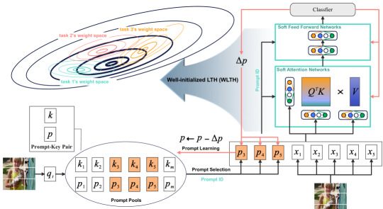
Leveraged by the WLTH, this work proposes a new Soft-TransFormer (Soft-TF) to address fine-tuning with minimal CF, as shown in Figure 1. We could find task-specific soft-networks or subnetworks based on well-trained frozen transformer parameters that incrementally learn task-adaptive weights associated with each task scenario.
Our contributions can be summarized as follows:
-
•
Inspired by Well-initialized Lottery Ticket Hypothesis (WLTH), we propose a novel continual learning method referred to as Soft-TransFormers (Soft-TF), which learns compact task-specific soft-networks or subnetworks from well pre-trained parameters for each task.
-
•
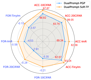
Extensive experiments demonstrate the Soft-TF leads to better generalized continual models than baselines such as DualPrompts, achieving state-of-the-art performances on various class-incremental learning (CIL) and task-incremental learning (TIL) scenarios, as shown in Figure 2.
 |
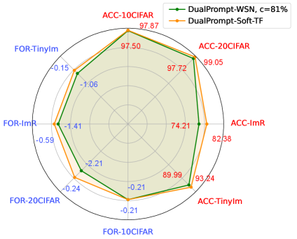 |
| (a) DualPrompt-PGP v.s. Soft-TransFormers (Soft-TF) | (b) DualPrompt-WSN v.s. Soft-TransFormers (Soft-TF) |
2 Related Works
Continual Learning (McCloskey & Cohen, 1989; Thrun, 1995; Kumar & Daume III, 2012; Li & Hoiem, 2016) is the challenge of learning a sequence of tasks continuously while utilizing and preserving previously learned knowledge to improve performance on new tasks. Four major approaches have been proposed to tackle the challenges of continual learning, such as catastrophic forgetting. One such approach is Regularization-based approaches (Kirkpatrick et al., 2017a; Chaudhry et al., 2020; Jung et al., 2020; Titsias et al., 2020; Mirzadeh et al., 2021), which aim to reduce catastrophic forgetting by imposing regularization constraints that inhibit changes to the weights or nodes associated with past tasks. Rehearsal-based approaches (Rebuffi et al., 2017; Chaudhry et al., 2019a; b; Saha et al., 2021; Deng et al., 2021; Sun et al., 2023; Sarfraz et al., 2023; Mai et al., 2021; Lin et al., 2023; Aljundi et al., 2019; Caccia et al., 2021; Chaudhry et al., 2019c; Liang & Li, 2024; Buzzega et al., 2020) store small data summaries to the past tasks and replay them during training to retain the acquired knowledge. Some approaches in this line of work (Shin et al., 2017; Aljundi et al., 2019) accommodate the generative model to construct the pseudo-rehearsals for previous tasks. Architecture-based approaches (Mallya et al., 2018; Serrà et al., 2018; Li et al., 2019; Wortsman et al., 2020; Kang et al., 2022; 2023; 2024b; 2024a) use the additional capacity to expand (Xu & Zhu, 2018; Yoon et al., 2018), dynamic representation (Yan et al., 2021; Singh et al., 2020) or isolate (Rusu et al., 2016) model parameters, preserving learned knowledge and preventing forgetting. Rehearsal and architecture-based methods have shown remarkable efficacy in suppressing catastrophic forgetting but require additional capacity for the task-adaptive parameters (Wortsman et al., 2020) or the replay buffers. Recently, Prompt-based approaches, an emerging transfer learning technique, harnesses a fixed function of pre-trained Transformer models. This empowers the language model to receive additional instructions for enhancing its performance on downstream tasks. Notably, while L2P (Wang et al., 2022c) stands out as the seminal work that bridges the gap between prompting and continual learning, DualPrompt (Wang et al., 2022b) introduces an innovative approach to affixing complementary prompts to the fixed pre-trained backbone. Here, we introduce a new approach to update the fixed pre-trained parameters through learnable sparse networks under the convergence theory, maximumly enabling the acquisition of task-invariant and task-specific instructions.
Prompt-based CL. With recent advances in Vision Transformers (Khan et al., 2022) and prompt-based fine-tuning in NLP (Li & Liang (2021)), Wang et al. (2022c) have shown that interacting with an ImageNet pre-trained model via prompt learning is a promising approach, L2P (Wang et al., 2022c) for continual learning (DualPrompt (Wang et al., 2022b), DyTox (Douillard et al., 2022), S-Prompt Wang et al. (2022a), CODA-P (Smith et al., 2023b), ConStruct-VL Smith et al. (2023a), ST-Prompt (Pei et al., 2023), and LGCL (Khan et al., 2023)). Recently, Prompt Gradient Projection (PGP) (Qiao et al., 2024), a small set of learnable orthogonal parameters, is appended to the input and enables quick adaptation of a frozen ImageNet pre-trained model to new streaming tasks. Their analysis shows that directly leveraging the pre-trained vision-language model without introducing any learnable parameters is a simple yet promising approach to continual learning. The PGP adopted a joint vision-language model like CLIP (Radford et al., 2021) for continual learning, which presents multiple advantages. It enables catering for practical scenarios with no well-defined task identities and boundaries, and the model is required to adapt to streaming data dynamically in a task-agnostic manner. However, prompt-based models come with several disadvantages. Poorly trained prompts could lead to suboptimal performance or tend to be biased. Moreover, prompt tuning could not capture all nuances of uncorrelated sequential tasks. These disadvantages lead to exploring alternative methods like full fine-tuning or hybrid approaches for more robust and flexible prompt-based model performance. In this work, to alleviate these issues, we investigate a fullly fine-tuning of well-pre-trained transformers on training soft networks and finding competitive subnetworks.
3 Prerequisites
We start with conventional prompt-based continual learning methods using Vision Transformer (ViT) (Dosovitskiy et al., 2020) and Contrastive Language-Image Pre-training (CLIP) (Radford et al., 2021) in Class Incremental Learning (CIL) and Task Incremental Learning (TIL) scenarios.
3.1 Preliminaries
Problem Statement. Continual Learning (CL) involves training deep neural networks (DNN) on time-variant data represented as a sequence of tasks, . Each -th task, consists of tuples where is an input sample and is the corresponding label. When a task arrives, a model is trained for the current task, while data from previous tasks is inaccessible. This work focuses primarily on class incremental learning (CIL), in which the task-ID is not given during inference.
Soft & Subnetworks have been explored in continual learning through two notable approaches. One approach, known as supermasks (Wortsman et al., 2020), produces outputs by , where denotes elementwise multiplication. In this method, the weights remain fixed at their initialization, with bias terms set to and other parameters initialized to with equal probability where the constant is the standard deviation of the corresponding Kaiming normal distribution (He et al., 2015). Another line of work includes WSN (Kang et al., 2022) and SoftNet (Kang et al., 2023), which jointly learn the model weights and task-adaptive subnetworks . The parameter-efficient reusable subnetworks are obtained by iteratively selecting the top- of the weights based on an importance score at each layer. WSN has primarily demonstrated its effectiveness in Convolutional Neural Networks (CNNs). However, its pruning mechanism for pre-trained Transformers, such as ViT, remains unexplored. To discover the competitive sparseness in Transformers, we detail the WSN-style task-adaptive fine-tuning and the learnable soft-networks of Transformers, presenting these adaptations for the first time with empirical observations. The soft-networks originate from learned parameters distributed with & various variances, as stated in Figure 6.
3.2 Prompt-based Class Incremental Learning (CIL)
A simple yet effective prompt-based (prompt-tuning) CIL model: Learning to Prompt (L2P) (Wang et al., 2022c) is first proposed. In this model, a prompt , a tiny set of trainable tokens combined with image features, is fed into the Vision Transformer (ViT) to help the model resist forgetting. To select suitable prompts for task-specific training, L2P utilizes a prompt pool containing numerous prompt-key pairs, , where represents the -th task prompt, represents the -th coresponding task key, and is the total number of prompt-key pairs.
Building on L2P, DualPrompt (Wang et al., 2022b) divided the prompts into expert (E-) prompts and general (G-) prompts for distinct features learning. DualPrompt also replaced prompt-tuning with prefix-tuning, which was successfully proven in NLP. DyTox (Douillard et al., 2022) designed a novel task attention block that utilized task tokens to infer task identifiers. Coda-Prompt (Smith et al., 2023b) replaced the prompt pool with a decomposed prompt, represented by a weighted sum of learnable prompt components, which optimized itself in an end-to-end fashion, providing high plasticity. LGCL (Khan et al., 2023) introduced text information into the learning of prompt pool, improving performance without any additional learnable parameters.
Recently, Qiao et al. (2024) introduced Prompt Gradient Projection (PGP), which applies an orthogonal condition on the prompt gradient to reduce forgetting via the self-attention mechanism in ViT effectively. Although various prompt-based continual learners have demonstrated state-of-the-art performance, they do not explicitly model task-specific fine-tuning and forgetting within the continual learning framework. In this work, we address task-specific fine-tuning and gradient-based task identification in CIL and TIL scenarios by leveraging prompt-tuning and learnable sparse networks.
4 Transformer with Learnable Subnetworks
In this section, we explain how Soft-TransFormers (Soft-TF) leverage learnable soft-networks to train sequential tasks while keeping the well-pretrained model parameters fixed. To introduce our novel Soft-TF and provide a clearer understanding, we draw on a partial explanation of DualPrompt.
4.1 Soft-MSA Layers
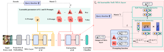
To address the task-specific fine-tuning of the pre-trained model, such as ViT, this work proposes a new Soft-TransFormer (Soft-TF), as illustrated in Figure 1. The proposed Soft-TF consists of a conventional neural network, like a multilayer transformer with multihead attention and forward networks. Using well-trained transformer parameters, we could discover task-specific soft-networks, as depicted in Figure 3. The Soft-TF incrementally learns model weights and task-adaptive soft-masks with well-pre-trained and soft-network parameters .
Given a pre-trained parameter and learnable soft-parameters , Soft-ViT is represented as , consisting of consecutive soft-MSA layers. We extend the notation by denoting the input embedding feature of the -th learnable soft-MSA layer as , where , and can refer to either the G-Prompt layer or the E-Prompt layer . Note that while the pre-trained parameters remain fixed, the soft-parameters are updated to provide task-specific solutions.
G-prompt. with sequence length and embedding dimension , is a shared parameter for all tasks. G-Prompt is attached to the -th MSA layer to transform via a prompting function as follows:
| (1) |
where defines the approach for attaching the prompt to the hidden embeddings.
E-prompt & Soft-networks. is a set of task-dependent parameters, where has as sequence length of and the same embedding dimension as the G-prompt, and is the total number of tasks. Unlike the shared G-prompt, each is associated with a task-specific key , which is also a learnable parameter aimed at capturing representative features of a task. For an input example from the -th task, to attach E-prompt to the -th soft-MSA layer, we apply the prompting function in a similar way:
| (2) |
4.2 Prompts with Learnable Subnetworks
G- and E-prompts, along with learnable soft-networks, encode specific types of instructions during training with the backbone and work together to guide the model’s predictions during inference. We have demonstrated the method for attaching prompts and learnable soft-networks to a single soft-MSA layer. Similarly to the approach taken in DualPrompt (Wang et al., 2022b), we also investigate layers of E-prompts with learnable soft-networks , while utilizing the layers designated for G-prompts.
Layers of G- and E-Prompts. We use the multilayered extension of both types of prompts: , where represents the G-prompt attached to the -th MSA layer. Similarly, we define for the -th conventional MSA layer. In this configuration, the G-prompt is attached from the -th to the -th conventional MSA layers, and the E-prompt is attached to the -th soft-MSA layers, ensuring that there is no overlap between them. In our experiments, we follow the () settings used in DualPrompt and empirically search for the optimal layers for the learnable subnetworks through ablation studies.
Learnable Soft-networks. The prompting function determines how prompts () are combined with fine-tuned soft () embedding features. From another perspective, directly influences the interaction between high-level instructions in the prompts and low-level representations. Therefore, we believe that a well-designed prompting function, along with task-specific parameters, is crucial for optimizing overall continual learning performance.
Specifically, applying a prompting and fine-tuning function can be seen as modifying the inputs to the soft-MSA layers. Let the input to the soft-MSA layer be , and denote the input query, key, and values for the soft-MSA layer as , , and , respectively. A soft-MSA layer is defined by the following equation:
| (3) | ||||
where , and are fixed projection matrices while , and are learnable parameters. is the number of heads. In ViT, . Here, we define a unified prompt parameter with a sequence length of , such as for a single-layered G- or E-prompt.
4.3 Fine-tuning on Well-initialized Parameters
In this framework, we concatenate the prompts and the embedding sequence , i.e., inputs from -th task, along the embedding dimension: . With the weights of , the soft-transformer takes query () and key () as input of the soft-MSA layer. The soft-attention matrix is then given by:
| (4) |
where we focus on and . First, the trainable prompt parameters can be denoted as:
| (5) |
Second, the trainable soft-attention layer’s parameters with and are as follows:
| (6) |
where and are frozen and unchanged during training and test.
4.4 The Optimization of Soft-Transformers
The overall process of the Soft-TransFormers (Soft-TF) during training and testing is described as Algorithm 1 and Algorithm 2. We denote the architecture with attached prompts as . The input of the -th task is transformed using and then passed to the classification head , parameterized by , for prediction. Finally, we train the two prompts, the task keys, the soft-attention parameters, and the newly-initialized classification head in an end-to-end manner:
| (7) |
Here, represents the cross-entropy loss, and denotes the matching loss, where corresponds to the feature vector associated with the [class] token (Dosovitskiy et al., 2020; Wang et al., 2022b), and is the cosine similarity. The scalar serves as a balancing factor between the losses; here, we follow the same DualPrompt setting as a baseline.
Analysis of Soft-TF for Convex-Lipschitz Functions. To analyze the convergence rate of the Soft-Transformer, we focus on the case of convex-Lipschitz functions. Let be any vector, and let be an upper bound on when , or is an initial state. It is helpful to consider as the minimizer of , although the following analysis applies to any .
We derive an upper bound on the sub-optimality of our solution relative to , specifically , where . By the definition of and applying Jensen’s inequality, we obtain the following (see Section A.1 stated in detail):
| (8) | ||||
For every , because of the convexity of , we have that
| (9) |
Combining the preceding, we obtain
| (10) |
To bound the right-hand side of the above formula, we rely on the following lemma:
Lemma 4.1.
Let be an arbitrary sequence of vectors, such as the -th task gradients . Consider any algorithm with a well-initialized (well pre-trained Transformer from WLTH) starting point and an update rule of the form:
| (11) |
satisfies with
| (12) | ||||
where since is learnable parameters in Soft-TransFormers. Specifically, we could assume that and of Equation 6 and are here frozen pre-trained parameters.
Theorem 4.2.
For every where and , if for all we have that and we set with large enough , then for every with we have
| (13) |
5 Experiments
We validate our method on several benchmark datasets against continuous learning baselines in Class-Incremental Learning (CIL) and Task-Incremental Learning (TIL).
5.1 Experimental Settings
Datasets. We evaluate our method mainly on 1) 10/20-Split-CIFAR100 (Krizhevsky et al., 2009), constructed by splitting the 100 classes into 10 tasks/20 tasks. 2) 10-Split-TinyImageNet (Abai & Rajmalwar, 2019), constructed by splitting the 200 classes into 10 tasks. 3) 10-Split-ImageNet-R (Hendrycks et al., 2021), constructed by splitting the 200 classes into 10 tasks. To show our effectiveness, we additionally compare our method with the baselines on 5-Split-CUB200 and 10-Split-TinyImageNet. The detailed experimental settings are depicted in the Supplementary.
Implementation. For fair comparisons, we set L2P (Wang et al., 2022c), DualPrompt (Wang et al., 2022b), CLIP (Radford et al., 2021), and PGP (Qiao et al., 2024) as our baselines. We follow experimental settings Qiao et al. (2024) entirely.
Baselines. To validate the powerfulness of our method, we compare our results with various CIL baselines including ICaRL (Rebuffi et al., 2017), BiC (Wu et al., 2019), DER++ (Buzzega et al., 2020), LWF (Li & Hoiem, 2017), EWC (Kirkpatrick et al., 2017b), DER+MCG (Cai et al., 2023), and DualPrompt-PGP (Qiao et al., 2024). In addition, we investigate subnetwork solutions such as WSN (Kang et al., 2022) (obtained by selecting top- of weight scores while fixing pre-trained parameters) and SoftNet (Kang et al., 2023) (acquired by selecting top- of weight scores as major tickets while setting as minor tickets) in Vision Transformers (ViT) using prompt tuning methods. We adopt average accuracy (ACC) and forgetting (FOR) as our validation metrics (Wang et al., 2022b; Qiao et al., 2024).
Task Inference. At the inference time, we infer task identity for arbitrary pieces of task samples for finding the proper task nuances and demonstrating full fine-tuning results. We summarize the following two methods:
-
•
Prompt ID: For a test example , we simply choose the best matched task index via .
-
•
Gradient ID: To infer the task identity, we follow SupSup’s one-shot task inference (Wortsman et al., 2020). In short, we assign each learned subnetwork a weight such that and when evaluating all seen tasks. Given an example data point of batch to classify, we can compute the loss as where is the pre-trained model which outputs logits and is the entropy function. From here our inferred task is simply .
| 10-Split-CIFAR100 | 20-Split-CIFAR100 | 10-Split-ImageNet-R | ||||||
| Method | Exemplar | Task ID | ACC() | Forget() | ACC() | Forget() | ACC() | Forget() |
| BiC | 5,000 | - | 81.42 | 17.31 | 73.02 | 6.23 | 64.63 | 22.25 |
| DER++ | 5,000 | - | 83.94 | 14.55 | - | - | 66.73 | 20.67 |
| iCaRL | 5,000 | - | 66.00 | 5.33 | 78.02 | 5.80 | - | - |
| DER+MCG | 2,000 | - | 67.62 | 14.64 | 65.84 | 13.72 | - | - |
| BiC | 1,000 | - | 66.11 | 35.24 | 63.12 | 21.89 | 52.14 | 36.70 |
| DER++ | 1,000 | - | 61.06 | 39.87 | - | - | 55.47 | 34.64 |
| iCaRL | 1,000 | - | 61.25 | 14.19 | 71.32 | 15.98 | - | - |
| FT | - | - | 33.61 | 86.87 | 33.52 | 53.69 | 28.87 | 63.80 |
| EWC | - | - | 47.01 | 33.27 | 36.73 | 35.19 | 35.00 | 56.16 |
| LWF | - | - | 60.69 | 27.77 | 39.12 | 57.91 | 38.54 | 52.37 |
| L2P∗ | - | Prompt ID | 83.77 | 6.63 | 71.29 | 13.96 | 60.44 | 9.00 |
| L2P-PGP∗ | - | Prompt ID | 84.34 | 5.59 | 76.12 | 13.26 | 61.40 | 8.03 |
| L2P-PGP-Soft-TF | - | Prompt ID | 86.26 | 4.79 | 76.17 | 15.77 | 69.80 | 5.13 |
| L2P-PGP-Soft-TF | - | Gradient ID | 86.46 | 4.87 | 77.67 | 15.84 | 69.56 | 5.28 |
| DualPrompt-PGP | - | Prompt ID | 86.92 | 5.35 | 83.74 | 7.91 | 69.34 | 4.53 |
| DualPrompt-PGP-Soft-TF | - | Prompt ID | 92.41 | 2.44 | 95.14 | 1.90 | 74.65 | 4.39 |
| DualPrompt-PGP-Soft-TF | - | Gradient ID | 92.92 | 2.34 | 95.89 | 1.64 | 81.45 | 2.89 |
| DualPrompt | - | Prompt ID | 86.50 | 5.77 | 82.98 | 8.20 | 68.13 | 4.46 |
| DualPrompt-Soft-TF | - | Prompt ID | 91.77 | 3.37 | 94.43 | 2.02 | 74.70 | 6.46 |
| DualPrompt-Soft-TF (SOTA) | - | Gradient ID | 97.87 | 0.21 | 99.05 | 0.24 | 82.38 | 0.59 |
| Upper-Bound of Soft-TF | - | - | 93.90 | - | 93.90 | - | 80.21 | - |
| 10-Split-CIFAR100 | 5-Split-CUB200 | |||||
| Method | Pretrained-dataset | Task ID | ACC() | Forget() | ACC() | Forget() |
| DualPrompt | ImageNet-21K | Prompt ID | 86.50 | 5.77 | 82.02 | 4.23 |
| DualPrompt-PGP | ImageNet-21K | Prompt ID | 86.92 | 5.35 | 82.46 | 3.76 |
| DualPrompt | SAM | Prompt ID | 86.11 | 6.08 | 82.02 | 4.73 |
| DualPrompt | DINO | Prompt ID | 64.18 | 23.81 | 50.88 | 10.10 |
| DualPrompt-Soft-TF | ImageNet-21K | Prompt ID | 92.42 | 2.44 | 76.17 | 9.04 |
| DualPrompt-Soft-TF (SOTA) | ImageNet-21K | Gradient ID | 97.87 | 0.21 | 87.93 | 0.66 |
| DualPrompt-Soft-TF (SOTA) | SAM | Gradient ID | 97.87 | 0.21 | 87.93 | 0.66 |
| DualPrompt-Soft-TF | DINO | Gradient ID | 84.50 | 12.27 | 69.79 | 10.93 |
| Upper-Bound of Soft-TF | - | - | 93.90 | - | 85.56 | - |
| Class Incremental | Task Incremental | |||||
| Method | Task ID | ACC() | Forget() | ACC() | Forget() | |
| CLIP | Prompt ID | 73.76 | 5.60 | 92.69 | 2.34 | |
| CLIP-PGP | Prompt ID | 79.47 | 4.23 | 93.00 | 1.58 | |
| CLIP∗ | Prompt ID | 74.60 | 7.75 | 93.59 | 2.80 | |
| CLIP-PGP∗ | Prompt ID | 74.63 | 7.76 | 93.67 | 2.83 | |
| CLIP-Prompt | Prompt ID | 70.27 | 12.95 | 93.36 | 3.07 | |
| CLIP-Prompt-Soft-TF-L[3,4,5] | Prompt ID | 71.58 | 7.73 | 95.29 | 1.12 | |
| CLIP-Prompt-Soft-TF-L[3,4,5] | Gradient ID | 76.77 | 5.59 | 95.29 | 1.12 | |
| CLIP-Prompt-Soft-TF-L[1-12] | Prompt ID | 72.28 | 3.44 | 96.83 | 0.44 | |
| CLIP-Prompt-Soft-TF-L[1-12] (SOTA) | Gradient ID | 85.90 | 3.07 | 96.83 | 0.44 | |
5.2 Performances
Performances of Soft-TF on CIL. We compare our Soft-TransFormers (Soft-TF) with state-of-the-art CIL baselines, as shown in Table 1. Our Soft-TF significantly outperforms all baselines and upper-bounds of Soft-TF, including L2P and DualPrompt, in both accuracy and forgetting measurements. The performance gain of Soft-TF is especially notable in DualPrompt-based learning compared to L2P, suggesting the importance of global prompt-tuning and multi-head attention prompt-tuning in DualPrompt. Additionally, task-identity inference using Gradient-ID is crucial for achieving full fine-tuning results in CIL. To demonstrate the effectiveness of Soft-TF, Figure 2(a) presents a radar chart comparing DualPrompt-PGP and Soft-TransFormers across four benchmark datasets.
Well-initialized LTH (WLTH) on CIL. To demonstrate the efficacy of our proposed method on Well-initialized Lottery Ticket Hypothesis (WLTH) backbones, we evaluate our Soft-TransFormers (Soft-TF) by extending two distinct pre-trained models, ViT-DINO and ViT-SAM (Caron et al., 2021; Chen et al., 2021). As shown in Table 2, we tested our method on the 10-Split-CIFAR100 and 5-Split-CUB200 datasets using three pre-trained ViTs: ImageNet-21K, DINO, and SAM, further validating the effectiveness of our approach on non-ImageNet datasets (Krizhevsky et al., 2009; Wah et al., 2011). Surprisingly, when initialized with ImageNet-21K and SAM, DualPrompt-Soft-TF with ImageNet-21K achieved the same performance levels. Moreover, DualPrompt-Soft-TF outperformed all baselines, i.e., DualPrompt-PGP, on both benchmark datasets, indicating that well-initialized weights provide better generalization in continual learning scenarios.
CLIP on CIL and TIL. We conduct our experiments on the 10-Split-CIFAR100 dataset under both Class Incremental Learning (CIL) and Task Incremental Learning (TIL) settings, as shown in Table 3. The results demonstrate that CLIP-Prompt-Soft-TF-L[1-12] significantly improves performance in both settings, indicating that our Soft-TF with Gradient ID is also effective in vision-language models, thereby broadening its applicability.
5.3 Ablation Studies
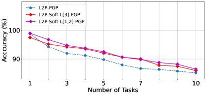
Layer-wise Inspections. We analyze the layer-wise performance of Soft-Transformer with respect to L2P and DualPrompt on the 10-Split-CIFAR100 dataset to identify the optimal configurations, as shown in Figure 4. Our observations reveal that the global prompt in DualPrompt influences Soft-Transformer’s performance differently in L2P and DualPrompt settings. In L2P-PGP, the best performance was achieved with Soft-TransFormers applied to the lower layers ((a) L2P-Soft-TF-L[1,2]-PGP), whereas in DualPrompt, the higher layers ((b) DualPrompt-Soft-TF-L[10,11,12]) yielded the best results. Notably, DualPrompt-Soft-TF-L[10,11,12] without PGP demonstrated impressive performance, achieving almost zero forgetting (0.21). These findings suggest that our approach could significantly enhance the effectiveness of large-scale Transformer models in continual learning scenarios.
 |
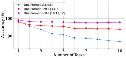 |
| (a) L2P-PGP v.s. Soft-Transformer | (b) DualPrompt v.s. Soft-Transformer |
6 Conclusion
Inspired by Well-initialized Lottery Ticket Hypothesis (WLTH) that provides suboptimal fine-tuning solutions, we proposed a novel fully fine-tuned continual learning (CL) method referred to as Soft-TransFormers (Soft-TF), which sequentially learns and selects an optimal soft-network or subnetwork for each task. In training, Soft-TF jointly learned the sparse layer’s weights in CL to obtain task-adaptive soft(real-valued)-networks or subnetworks (binary masks) while freezing the well-pre-trained layer parameters. In inference, the identified task-adaptive network of Soft-TF, which masks the parameters of the pre-trained network, maps to an optimal solution associated with each task, minimizing Catastrophic Forgetting (CF)—the soft masking was immune to the pre-trained network’s knowledge forgetting. Extensive experiments demonstrated the power of Soft-TF (Vision Transformer and CLIP) and show state-of-the-art performances with convergence theory in various CL scenarios, i.e., Class-Incremental Learning (CIL) and Task-Incremental Learning (TIL).
References
- Abai & Rajmalwar (2019) Zoheb Abai and Nishad Rajmalwar. Densenet models for tiny imagenet classification. arXiv preprint arXiv:1904.10429, 2019.
- Aljundi et al. (2019) Rahaf Aljundi, Eugene Belilovsky, Tinne Tuytelaars, Laurent Charlin, Massimo Caccia, Min Lin, and Lucas Page-Caccia. Online continual learning with maximal interfered retrieval. In Advances in Neural Information Processing Systems (NeurIPS), 2019.
- Buzzega et al. (2020) Pietro Buzzega, Matteo Boschini, Angelo Porrello, Davide Abati, and Simone Calderara. Dark experience for general continual learning: a strong, simple baseline. Advances in neural information processing systems, 33:15920–15930, 2020.
- Caccia et al. (2021) Lucas Caccia, Rahaf Aljundi, Nader Asadi, Tinne Tuytelaars, Joelle Pineau, and Eugene Belilovsky. New insights on reducing abrupt representation change in online continual learning. arXiv preprint arXiv:2104.05025, 2021.
- Cai et al. (2023) Tenghao Cai, Zhizhong Zhang, Xin Tan, Yanyun Qu, Guannan Jiang, Chengjie Wang, and Yuan Xie. Multi-centroid task descriptor for dynamic class incremental inference. In Proceedings of the IEEE/CVF Conference on Computer Vision and Pattern Recognition, pp. 7298–7307, 2023.
- Caron et al. (2021) Mathilde Caron, Hugo Touvron, Ishan Misra, Hervé Jégou, Julien Mairal, Piotr Bojanowski, and Armand Joulin. Emerging properties in self-supervised vision transformers. In Proceedings of the IEEE/CVF international conference on computer vision, pp. 9650–9660, 2021.
- Chaudhry et al. (2019a) Arslan Chaudhry, Marc’Aurelio Ranzato, Marcus Rohrbach, and Mohamed Elhoseiny. Efficient lifelong learning with a-gem. In Proceedings of the International Conference on Learning Representations (ICLR), 2019a.
- Chaudhry et al. (2019b) Arslan Chaudhry, Marcus Rohrbach, Mohamed Elhoseiny, Thalaiyasingam Ajanthan, Puneet K Dokania, Philip HS Torr, and M Ranzato. Continual learning with tiny episodic memories. arXiv preprint arXiv:1902.10486, 2019b.
- Chaudhry et al. (2019c) Arslan Chaudhry, Marcus Rohrbach, Mohamed Elhoseiny, Thalaiyasingam Ajanthan, Puneet K Dokania, Philip HS Torr, and Marc’Aurelio Ranzato. On tiny episodic memories in continual learning. arXiv preprint arXiv:1902.10486, 2019c.
- Chaudhry et al. (2020) Arslan Chaudhry, Naeemullah Khan, Puneet K Dokania, and Philip HS Torr. Continual learning in low-rank orthogonal subspaces. In Advances in Neural Information Processing Systems (NeurIPS), 2020.
- Chen et al. (2021) Xiangning Chen, Cho-Jui Hsieh, and Boqing Gong. When vision transformers outperform resnets without pre-training or strong data augmentations. arXiv preprint arXiv:2106.01548, 2021.
- Deng et al. (2021) Danruo Deng, Guangyong Chen, Jianye Hao, Qiong Wang, and Pheng-Ann Heng. Flattening sharpness for dynamic gradient projection memory benefits continual learning. In Advances in Neural Information Processing Systems (NeurIPS), 2021.
- Dosovitskiy et al. (2020) Alexey Dosovitskiy, Lucas Beyer, Alexander Kolesnikov, Dirk Weissenborn, Xiaohua Zhai, Thomas Unterthiner, Mostafa Dehghani, Matthias Minderer, Georg Heigold, Sylvain Gelly, et al. An image is worth 16x16 words: Transformers for image recognition at scale. arXiv preprint arXiv:2010.11929, 2020.
- Douillard et al. (2022) Arthur Douillard, Alexandre Ramé, Guillaume Couairon, and Matthieu Cord. Dytox: Transformers for continual learning with dynamic token expansion. In Proceedings of the IEEE/CVF Conference on Computer Vision and Pattern Recognition, pp. 9285–9295, 2022.
- Hassabis et al. (2017) Demis Hassabis, Dharshan Kumaran, Christopher Summerfield, and Matthew Botvinick. Neuroscience-inspired artificial intelligence. Neuron, 95(2):245–258, 2017.
- He et al. (2015) Kaiming He, Xiangyu Zhang, Shaoqing Ren, and Jian Sun. Delving deep into rectifiers: Surpassing human-level performance on imagenet classification. In Proceedings of the IEEE international conference on computer vision, pp. 1026–1034, 2015.
- Hendrycks et al. (2021) Dan Hendrycks, Steven Basart, Norman Mu, Saurav Kadavath, Frank Wang, Evan Dorundo, Rahul Desai, Tyler Zhu, Samyak Parajuli, Mike Guo, et al. The many faces of robustness: A critical analysis of out-of-distribution generalization. In Proceedings of the IEEE/CVF international conference on computer vision, pp. 8340–8349, 2021.
- Houlsby et al. (2019) Neil Houlsby, Andrei Giurgiu, Stanislaw Jastrzebski, Bruna Morrone, Quentin De Laroussilhe, Andrea Gesmundo, Mona Attariyan, and Sylvain Gelly. Parameter-efficient transfer learning for nlp. In International conference on machine learning, pp. 2790–2799. PMLR, 2019.
- Hu et al. (2021) Edward J Hu, Yelong Shen, Phillip Wallis, Zeyuan Allen-Zhu, Yuanzhi Li, Shean Wang, Lu Wang, and Weizhu Chen. Lora: Low-rank adaptation of large language models. arXiv preprint arXiv:2106.09685, 2021.
- Jung et al. (2020) Sangwon Jung, Hongjoon Ahn, Sungmin Cha, and Taesup Moon. Continual learning with node-importance based adaptive group sparse regularization. In Advances in Neural Information Processing Systems (NeurIPS), 2020.
- Kang et al. (2022) Haeyong Kang, Rusty John Lloyd Mina, Sultan Rizky Hikmawan Madjid, Jaehong Yoon, Mark Hasegawa-Johnson, Sung Ju Hwang, and Chang D Yoo. Forget-free continual learning with winning subnetworks. In International Conference on Machine Learning, pp. 10734–10750. PMLR, 2022.
- Kang et al. (2023) Haeyong Kang, Jaehong Yoon, Sultan Rizky Hikmawan Madjid, Sung Ju Hwang, and Chang D. Yoo. On the soft-subnetwork for few-shot class incremental learning. In The Eleventh International Conference on Learning Representations, 2023. URL https://openreview.net/forum?id=z57WK5lGeHd.
- Kang et al. (2024a) Haeyong Kang, Jaehong Yoon, Sung Ju Hwang, and Chang D. Yoo. Continual learning: Forget-free winning subnetworks for video representations, 2024a. URL https://arxiv.org/abs/2312.11973.
- Kang et al. (2024b) Haeyong Kang, Jaehong Yoon, DaHyun Kim, Sung Ju Hwang, and Chang D. Yoo. Progressive fourier neural representation for sequential video compilation. In The Twelfth International Conference on Learning Representations, 2024b. URL https://openreview.net/forum?id=rGFrRMBbOq.
- Khan et al. (2023) Muhammad Gul Zain Ali Khan, Muhammad Ferjad Naeem, Luc Van Gool, Didier Stricker, Federico Tombari, and Muhammad Zeshan Afzal. Introducing language guidance in prompt-based continual learning. In Proceedings of the IEEE/CVF International Conference on Computer Vision, pp. 11463–11473, 2023.
- Khan et al. (2022) Salman Khan, Muzammal Naseer, Munawar Hayat, Syed Waqas Zamir, Fahad Shahbaz Khan, and Mubarak Shah. Transformers in vision: A survey. ACM computing surveys (CSUR), 54(10s):1–41, 2022.
- Kirkpatrick et al. (2017a) James Kirkpatrick, Razvan Pascanu, Neil Rabinowitz, Joel Veness, Guillaume Desjardins, Andrei A Rusu, Kieran Milan, John Quan, Tiago Ramalho, Agnieszka Grabska-Barwinska, Demis Hassabis, Claudia Clopath, Dharshan Kumaran, and Raia Hadsell. Overcoming catastrophic forgetting in neural networks. 2017a.
- Kirkpatrick et al. (2017b) James Kirkpatrick, Razvan Pascanu, Neil Rabinowitz, Joel Veness, Guillaume Desjardins, Andrei A Rusu, Kieran Milan, John Quan, Tiago Ramalho, Agnieszka Grabska-Barwinska, et al. Overcoming catastrophic forgetting in neural networks. Proceedings of the national academy of sciences, 114(13):3521–3526, 2017b.
- Krizhevsky et al. (2009) Alex Krizhevsky, Geoffrey Hinton, et al. Learning multiple layers of features from tiny images. 2009.
- Kumar & Daume III (2012) Abhishek Kumar and Hal Daume III. Learning task grouping and overlap in multi-task learning. In Proceedings of the International Conference on Machine Learning (ICML), 2012.
- Li & Liang (2021) Xiang Lisa Li and Percy Liang. Prefix-tuning: Optimizing continuous prompts for generation. arXiv preprint arXiv:2101.00190, 2021.
- Li et al. (2019) Xilai Li, Yingbo Zhou, Tianfu Wu, Richard Socher, and Caiming Xiong. Learn to grow: A continual structure learning framework for overcoming catastrophic forgetting. In Proceedings of the International Conference on Machine Learning (ICML), 2019.
- Li & Hoiem (2016) Zhizhong Li and Derek Hoiem. Learning without forgetting. In Proceedings of the European Conference on Computer Vision (ECCV), 2016.
- Li & Hoiem (2017) Zhizhong Li and Derek Hoiem. Learning without forgetting. IEEE transactions on pattern analysis and machine intelligence, 40(12):2935–2947, 2017.
- Liang & Li (2024) Yan-Shuo Liang and Wu-Jun Li. Loss decoupling for task-agnostic continual learning. Advances in Neural Information Processing Systems, 36, 2024.
- Lin et al. (2023) Huiwei Lin, Baoquan Zhang, Shanshan Feng, Xutao Li, and Yunming Ye. Pcr: Proxy-based contrastive replay for online class-incremental continual learning. In Proceedings of the IEEE/CVF Conference on Computer Vision and Pattern Recognition, pp. 24246–24255, 2023.
- Mai et al. (2021) Zheda Mai, Ruiwen Li, Hyunwoo Kim, and Scott Sanner. Supervised contrastive replay: Revisiting the nearest class mean classifier in online class-incremental continual learning. In Proceedings of the IEEE/CVF Conference on Computer Vision and Pattern Recognition, pp. 3589–3599, 2021.
- Mallya et al. (2018) Arun Mallya, Dillon Davis, and Svetlana Lazebnik. Piggyback: Adapting a single network to multiple tasks by learning to mask weights. In Proceedings of the European Conference on Computer Vision (ECCV), 2018.
- McCloskey & Cohen (1989) Michael McCloskey and Neal J Cohen. Catastrophic interference in connectionist networks: The sequential learning problem. In Psychology of learning and motivation, volume 24, pp. 109–165. Elsevier, 1989.
- Mirzadeh et al. (2021) Seyed Iman Mirzadeh, Mehrdad Farajtabar, Dilan Gorur, Razvan Pascanu, and Hassan Ghasemzadeh. Linear mode connectivity in multitask and continual learning. In Proceedings of the International Conference on Learning Representations (ICLR), 2021.
- Pei et al. (2023) Yixuan Pei, Zhiwu Qing, Shiwei Zhang, Xiang Wang, Yingya Zhang, Deli Zhao, and Xueming Qian. Space-time prompting for video class-incremental learning. In Proceedings of the IEEE/CVF International Conference on Computer Vision (ICCV), pp. 11932–11942, October 2023.
- Qiao et al. (2024) Jingyang Qiao, zhizhong zhang, Xin Tan, Chengwei Chen, Yanyun Qu, Yong Peng, and Yuan Xie. Prompt gradient projection for continual learning. In The Twelfth International Conference on Learning Representations, 2024. URL https://openreview.net/forum?id=EH2O3h7sBI.
- Radford et al. (2021) Alec Radford, Jong Wook Kim, Chris Hallacy, Aditya Ramesh, Gabriel Goh, Sandhini Agarwal, Girish Sastry, Amanda Askell, Pamela Mishkin, Jack Clark, et al. Learning transferable visual models from natural language supervision. In International conference on machine learning, pp. 8748–8763. PMLR, 2021.
- Rebuffi et al. (2017) Sylvestre-Alvise Rebuffi, Alexander Kolesnikov, Georg Sperl, and Christoph H Lampert. icarl: Incremental classifier and representation learning. In Proceedings of the IEEE conference on Computer Vision and Pattern Recognition, pp. 2001–2010, 2017.
- Riemer et al. (2018) Matthew Riemer, Ignacio Cases, Robert Ajemian, Miao Liu, Irina Rish, Yuhai Tu, and Gerald Tesauro. Learning to learn without forgetting by maximizing transfer and minimizing interference. arXiv preprint arXiv:1810.11910, 2018.
- Rusu et al. (2016) Andrei A Rusu, Neil C Rabinowitz, Guillaume Desjardins, Hubert Soyer, James Kirkpatrick, Koray Kavukcuoglu, Razvan Pascanu, and Raia Hadsell. Progressive neural networks. arXiv preprint arXiv:1606.04671, 2016.
- Saha et al. (2021) Gobinda Saha, Isha Garg, and Kaushik Roy. Gradient projection memory for continual learning. In Proceedings of the International Conference on Learning Representations (ICLR), 2021.
- Sarfraz et al. (2023) Fahad Sarfraz, Elahe Arani, and Bahram Zonooz. Error sensitivity modulation based experience replay: Mitigating abrupt representation drift in continual learning. In The Eleventh International Conference on Learning Representations, 2023. URL https://openreview.net/forum?id=zlbci7019Z3.
- Serrà et al. (2018) Joan Serrà, Didac Suris, Marius Miron, and Alexandros Karatzoglou. Overcoming catastrophic forgetting with hard attention to the task. In Proceedings of the International Conference on Machine Learning (ICML), 2018.
- Shalev-Shwartz & Ben-David (2014) Shai Shalev-Shwartz and Shai Ben-David. Understanding machine learning: From theory to algorithms. Cambridge university press, 2014.
- Shin et al. (2017) Hanul Shin, Jung Kwon Lee, Jaehon Kim, and Jiwon Kim. Continual learning with deep generative replay. In Advances in Neural Information Processing Systems (NeurIPS), 2017.
- Singh et al. (2020) Pravendra Singh, Vinay Kumar Verma, Pratik Mazumder, Lawrence Carin, and Piyush Rai. Calibrating cnns for lifelong learning. Advances in Neural Information Processing Systems, 33:15579–15590, 2020.
- Smith et al. (2023a) James Seale Smith, Paola Cascante-Bonilla, Assaf Arbelle, Donghyun Kim, Rameswar Panda, David Cox, Diyi Yang, Zsolt Kira, Rogerio Feris, and Leonid Karlinsky. Construct-vl: Data-free continual structured vl concepts learning. In Proceedings of the IEEE/CVF Conference on Computer Vision and Pattern Recognition (CVPR), pp. 14994–15004, June 2023a.
- Smith et al. (2023b) James Seale Smith, Leonid Karlinsky, Vyshnavi Gutta, Paola Cascante-Bonilla, Donghyun Kim, Assaf Arbelle, Rameswar Panda, Rogerio Feris, and Zsolt Kira. Coda-prompt: Continual decomposed attention-based prompting for rehearsal-free continual learning. In Proceedings of the IEEE/CVF Conference on Computer Vision and Pattern Recognition (CVPR), pp. 11909–11919, June 2023b.
- Sun et al. (2023) Wenju Sun, Qingyong Li, Jing Zhang, Wen Wang, and Yangli-ao Geng. Decoupling learning and remembering: A bilevel memory framework with knowledge projection for task-incremental learning. In Proceedings of the IEEE/CVF Conference on Computer Vision and Pattern Recognition, pp. 20186–20195, 2023.
- Thrun (1995) Sebastian Thrun. A Lifelong Learning Perspective for Mobile Robot Control. Elsevier, 1995.
- Titsias et al. (2020) Michalis K Titsias, Jonathan Schwarz, Alexander G de G Matthews, Razvan Pascanu, and Yee Whye Teh. Functional regularisation for continual learning with gaussian processes. In Proceedings of the International Conference on Learning Representations (ICLR), 2020.
- Wah et al. (2011) Catherine Wah, Steve Branson, Peter Welinder, Pietro Perona, and Serge Belongie. The caltech-ucsd birds-200-2011 dataset. 2011.
- Wang et al. (2022a) Yabin Wang, Zhiwu Huang, and Xiaopeng Hong. S-prompts learning with pre-trained transformers: An occam’s razor for domain incremental learning. Advances in Neural Information Processing Systems, 35:5682–5695, 2022a.
- Wang et al. (2022b) Zifeng Wang, Zizhao Zhang, Sayna Ebrahimi, Ruoxi Sun, Han Zhang, Chen-Yu Lee, Xiaoqi Ren, Guolong Su, Vincent Perot, Jennifer Dy, et al. Dualprompt: Complementary prompting for rehearsal-free continual learning. In European Conference on Computer Vision, pp. 631–648. Springer, 2022b.
- Wang et al. (2022c) Zifeng Wang, Zizhao Zhang, Chen-Yu Lee, Han Zhang, Ruoxi Sun, Xiaoqi Ren, Guolong Su, Vincent Perot, Jennifer Dy, and Tomas Pfister. Learning to prompt for continual learning. In Proceedings of the IEEE/CVF Conference on Computer Vision and Pattern Recognition, pp. 139–149, 2022c.
- Wortsman et al. (2020) Mitchell Wortsman, Vivek Ramanujan, Rosanne Liu, Aniruddha Kembhavi, Mohammad Rastegari, Jason Yosinski, and Ali Farhadi. Supermasks in superposition. In Advances in Neural Information Processing Systems (NeurIPS), 2020.
- Wu et al. (2019) Yue Wu, Yinpeng Chen, Lijuan Wang, Yuancheng Ye, Zicheng Liu, Yandong Guo, and Yun Fu. Large scale incremental learning. In Proceedings of the IEEE/CVF conference on computer vision and pattern recognition, pp. 374–382, 2019.
- Xu & Zhu (2018) Ju Xu and Zhanxing Zhu. Reinforced continual learning. In Advances in Neural Information Processing Systems (NeurIPS), 2018.
- Yan et al. (2021) Shipeng Yan, Jiangwei Xie, and Xuming He. Der: Dynamically expandable representation for class incremental learning. In Proceedings of the IEEE/CVF Conference on Computer Vision and Pattern Recognition, pp. 3014–3023, 2021.
- Yoon et al. (2018) Jaehong Yoon, Eunho Yang, Jeongtae Lee, and Sung Ju Hwang. Lifelong learning with dynamically expandable networks. In Proceedings of the International Conference on Learning Representations (ICLR), 2018.
- Zenke et al. (2017) Friedemann Zenke, Ben Poole, and Surya Ganguli. Continual learning through synaptic intelligence. In International Conference on Machine Learning, pp. 3987–3995. PMLR, 2017.
Appendix A Appendix
A.1 Analysis of Soft-TransFormers (Soft-TF)
Analysis of Soft-TransFormers for Convex-Lipschitz Functions. To analyze the convergence rate of the Soft-TransFormers (Soft-TF), we limit ourselves to the case of convex-Lipshitz functions along with the analysis (Shalev-Shwartz & Ben-David, 2014). Let be any vector or an optimal solution and let be an upper bound on when . It is convenient to think of as the minimizer of , but the analysis that follows holds for every .
We would like to obtain an upper bound on the sub-optimality of our solution with respect to , namely, , where . From the definition of , and using Jensen’s inequality, we have that
| (14) | ||||
For every , because of the convexity of , we have that
| (15) |
Combining the preceeding we obtain
| (16) |
To bound the right-hand side we rely on the following lemma:
Lemma A.1.
Let be an arbitrary sequence of vectors. Any algorithm with an well initialization (pre-trained model) and an update rule of the form
| (17) |
satisfies with
| (18) | ||||
where since is learnable parameters in Soft-TransFormers. Specifically, we could assume that and of Equation 6.
Theorem A.2.
For every where and , if for all we have that and if we set , then for every with we have
| (19) |
Proof.
Using algebraic manipulations (completing the square), we obtain:
| (20) | ||||
where the last equality follows from the definition of the update rule. Summing the equality over , we have
| (21) |
The first sum on the right-hand side is a telescopic sum that collapses to
| (22) |
Plugging this in Equation, we have
| (23) | ||||
where the last equality is due to the definition . This proves the first part of the lemma. The second part follows by upper bounding by , by , deciding by , and plugging in the value of .
In terms of Soft-TransFormers of Equation 6, we have
| (24) | ||||
where is an arbitrary -th vector and since and are pre-trained parameters.
however, in term of prompt , we have
| (25) | ||||
where is an arbitrary -th vector of prompt and since and are pre-trained parameters, and , respectively.
Therefore, we have from
| (26) | ||||
where since all are learnable parameters. For every where and , if for all we have that and if we set with large enough , then for every with we have
| (27) |
∎
A.2 Experimental Details
For fair comparisons with the baselines (Wang et al., 2022c; b; Qiao et al., 2024), we use ViT B/16 (Dosovitskiy et al., 2020) pre-trained on ImageNet-21K as our image encoder, which is kept frozen during training. We train and test on a single Quadro RTX 8000-48GB GPU for baselines and our Soft-TransFormers with Adam optimizer with and .
We adhere to the experimental settings outlined by Qiao et al. (2024) to validate our method’s effectiveness. When comparing our approach with L2P-PGP and Soft-Transformer on the 10/20-Split-CIFAR100 and 10-Split-TinyImageNet datasets, we train the network for 5 epochs with a batch size of 16 and set the prompt length to 5. For the 10-Split-ImageNet-R dataset, we use 50 epochs, a batch size of 16, and a prompt length of 30. In comparison with DualPrompt-PGP and Soft-TransFormers on the 10/20-Split-CIFAR100 dataset, we train the network for 20 epochs with a batch size of 24 and set the expert prompt length to 5. For the 10-Split-TinyImageNet dataset, we use 5 epochs, a batch size of 24, and an expert prompt length of 5. For the 10-Split-ImageNet-R dataset, we set the epochs to 50, the batch size to 24, and the expert prompt length to 20. Additionally, in all benchmark data sets, the general prompt length is set to 5, and the location inserted into the prompt is kept consistent.
For CLIP-PGP and Soft-TransFormers, we configure a single trainable image prompt that is shared across all tasks within the vision encoder. For the text encoder, following the approach of Qiao et al. (2024), we set a trainable text prompt for each class, which is only trained on the corresponding task. In our comparisons with CLIP-PGP and Soft-TransFormers on the 10-Split-CIFAR100 dataset, we set the image prompt length to 5, the number of epochs to 5, and the batch size to 32.
| 10-Split-CIFAR100 | 20-Split-CIFAR100 | 10-Split-ImageNet-R | ||||||
| Method | Exemplar | Task ID | ACC() | Forget() | ACC() | Forget() | ACC() | Forget() |
| BiC | 5,000 | - | 81.42 | 17.31 | 73.02 | 6.23 | 64.63 | 22.25 |
| DER++ | 5,000 | - | 83.94 | 14.55 | - | - | 66.73 | 20.67 |
| iCaRL | 5,000 | - | 66.00 | 5.33 | 78.02 | 5.80 | - | - |
| DER+MCG | 2,000 | - | 67.62 | 14.64 | 65.84 | 13.72 | - | - |
| BiC | 1,000 | - | 66.11 | 35.24 | 63.12 | 21.89 | 52.14 | 36.70 |
| DER++ | 1,000 | - | 61.06 | 39.87 | - | - | 55.47 | 34.64 |
| iCaRL | 1,000 | - | 61.25 | 14.19 | 71.32 | 15.98 | - | - |
| FT | - | - | 33.61 | 86.87 | 33.52 | 53.69 | 28.87 | 63.80 |
| EWC | - | - | 47.01 | 33.27 | 36.73 | 35.19 | 35.00 | 56.16 |
| LWF | - | - | 60.69 | 27.77 | 39.12 | 57.91 | 38.54 | 52.37 |
| L2P∗ | - | Prompt ID | 83.77 | 6.63 | 71.29 | 13.96 | 60.44 | 9.00 |
| L2P-PGP∗ | - | Prompt ID | 84.34 | 5.59 | 76.12 | 13.26 | 61.40 | 8.03 |
| L2P-PGP-Soft-TF | - | Prompt ID | 86.26 | 4.79 | 76.17 | 15.77 | 69.80 | 5.13 |
| L2P-PGP-Soft-TF | - | Gradient ID | 86.46 | 4.87 | 77.67 | 15.84 | 69.56 | 5.28 |
| DualPrompt | - | Prompt ID | 86.50 | 5.77 | 82.98 | 8.20 | 68.13 | 4.46 |
| DualPrompt-Soft-TF-L[3,4,5] | - | Prompt ID | 91.77 | 3.37 | 94.43 | 2.02 | 74.70 | 6.46 |
| DualPrompt-Soft-TF-L[3,4,5] | - | Gradient ID | 93.76 | 1.83 | 95.38 | 1.73 | 82.15 | 2.20 |
| DualPrompt-WSN-L[10,11,12], c=80.0% | - | Gradient ID | 97.41 | 0.18 | 90.25 | 9.08 | 74.83 | 0.91 |
| DualPrompt-WSN-L[10,11,12], c=81.0% | - | Gradient ID | 97.50 | 0.21 | 96.72 | 2.21 | 74.21 | 1.41 |
| DualPrompt-WSN-L[10,11,12], c=82.0% | - | Gradient ID | 97.67 | 0.27 | 96.44 | 1.62 | 75.02 | 0.92 |
| DualPrompt-WSN-L[10,11,12], c=83.0% | - | Gradient ID | 97.62 | 0.25 | 97.77 | 0.63 | 76.33 | 1.77 |
| DualPrompt-WSN-L[10,11,12], c=87.0% | - | Gradient ID | 97.51 | 0.27 | 97.68 | 0.75 | 77.96 | 1.02 |
| DualPrompt-WSN-L[10,11,12], c=90.0% | - | Gradient ID | 97.46 | 0.38 | 98.09 | 0.65 | 78.80 | 0.47 |
| DualPrompt-Soft-TF-L[10,11,12] | - | Gradient ID | 97.87 | 0.21 | 99.05 | 0.24 | 82.38 | 0.59 |
| DualPrompt-PGP | - | Prompt ID | 86.92 | 5.35 | 83.74 | 7.91 | 69.34 | 4.53 |
| DualPrompt-PGP-Soft-TF-L[3,4,5] | - | Prompt ID | 92.41 | 2.44 | 95.14 | 1.90 | 74.65 | 4.39 |
| DualPrompt-PGP-Soft-TF-L[3,4,5] | - | Gradient ID | 92.92 | 2.34 | 95.89 | 1.64 | 81.45 | 2.89 |
| Upper-Bound of DualPrompt | - | - | 90.85 | - | 90.85 | - | 79.13 | - |
| Upper-Bound of Soft-TF | - | - | 93.90 | - | 93.90 | - | 80.21 | - |
| 10-Split-CIFAR100 | |||||
| Method | Pretrained-Dataset | Task ID | Random Initialization | ACC() | Forget() |
| DualPrompt-Soft-TF-L[10,11,12] w/o FF | ImageNet-21K | Prompt ID | Xavier | 90.59 | 3.85 |
| DualPrompt-Soft-TF-L[10,11,12] w/o FF | ImageNet-21K | Prompt ID | Kaiming | 90.72 | 3.63 |
| DualPrompt-Soft-TF-L[10,11,12] w/o FF | ImageNet-21K | Prompt ID | Normal | 90.45 | 3.78 |
| DualPrompt-Soft-TF-L[10,11,12] w/o FF | ImageNet-21K | Prompt ID | Uniform(1.0, 1.0) | 92.35 | 2.98 |
| DualPrompt-Soft-TF-L[10,11,12] w/o FF | ImageNet-21K | Gradient ID | Uniform(1.0, 1.0) | 98.05 | 0.25 |
| Upper-Bound of Soft-TF | 93.90 | - | |||
Random initialization. Random initialization of Soft-Transformer’s weights plays a critical role when leveraging well-pretrained models like Vision Transformers (ViTs). The optimal training point is the parameters of a well-pretrained model. Among the initialization methods, Uniform initialization for Soft-TransFormer satisfies this requirement effectively. To validate these claims, we analyze the impact of common random initialization methods, including Xavier, Kaiming, Normal, and Uniform Initialization, as shown in Table 5. The results demonstrate that the same well-initialization point leads to independent optimal task performance, particularly with Gradient ID inference. Furthermore, this ablation study strengthens our Soft-TF with state-of-the-art-perfomances inspired by the Well-initialized Lottery Ticket Hypothesis (WLTH).
| Method | ViT-B/12 (85.8M) | 10-Split-CIFAR100 | 20-Split-CIFAR100 | 10-Split-ImageNet-R | ||||
| DualPrompt | # Train Params. | Task ID | Train (sec.) | Test (sec.) | Train (sec.) | Test (sec.) | Train (sec.) | Test (sec.) |
| DualPrompt | 0.00M | Prompt ID | 12.12K | 76 | 11.60K | 78 | 13.10K | 47 |
| PGP | 0.00M | Prompt ID | 12.21K | 76 | 13.12K | 78 | 13.33K | 47 |
| Soft-TF-L[12] w/ only ATTN | 1.76M | Gradient ID | 12.18K | 129 | 13.30K | 113 | 13.35K | 65 |
| Soft-TF-L[12] w/ only ATTN | 1.76M | Prompt ID | 12.18K | 78 | 13.30K | 80 | 13.35K | 48 |
| Soft-TF-L[12] w/o FF | 2.31M | Gradient ID | 12.24K | 103 | 13.40K | 132 | 13.42K | 66 |
| Soft-TF-L[11,12] w/o FF | 4.62M | Gradient ID | 12.95K | 115 | 14.38K | 146 | 14.23K | 73 |
| Soft-TF-L[10,11,12] w/o FF | 6.93M | Gradient ID | 13.71K | 130 | 15.51K | 163 | 15.08K | 82 |
| Soft-TF-L[10,11,12] w/o FF | 6.93M | Prompt ID | 13.87K | 80 | 15.60K | 104 | 15.35K | 52 |
| LoRA-L[10,11,12] w/o FF, r=4 | 0.06M | Prompt ID | 11.95K | 77 | 11.71K | 79 | 14.34K | 48 |
| LoRA-L[10,11,12] w/o FF, r=24 | 0.32M | Prompt ID | 12.03K | 78 | 15.10K | 100 | 15.02K | 50 |
| LoRA-L[10,11,12] w/o FF, r=500 | 6.91M | Prompt ID | 13.24K | 79 | 15.89K | 105 | 15.09K | 53 |
| Adapter-L[10,11,12] w/ FF, r=1 | 0.09M | Prompt ID | 12.44K | 84 | 12.40K | 81 | 14.40K | 50 |
| Adapter-L[10,11,12] w/ FF, r=4 | 0.36M | Prompt ID | 12.80K | 85 | 15.35K | 105 | 14.68K | 51 |
| Adapter-L[10,11,12] w/ FF, r=75 | 6.91M | Prompt ID | 13.66K | 88 | 15.72K | 106 | 15.50K | 53 |
| Method | ViT-B/12 (85.8M) | 10-Split-CIFAR100 | 20-Split-CIFAR100 | 10-Split-ImageNet-R | ||||
| DualPrompt | # Train Params. | Task ID | ACC() | Forget() | ACC() | Forget() | ACC() | Forget() |
| DualPrompt | 0.00M | Prompt ID | 86.50 | 5.77 | 82.98 | 8.20 | 68.13 | 4.46 |
| PGP | 0.00M | Prompt ID | 86.92 | 5.35 | 83.74 | 7.91 | 69.34 | 4.53 |
| Soft-TF-L[12] w/ only ATTN | 1.76M | Gradient ID | 97.17 | 0.40 | 98.09 | 0.54 | 72.31 | 3.94 |
| Soft-TF-L[12] w/ only ATTN | 1.76M | Prompt ID | 94.59 | 1.12 | 96.96 | 1.02 | 71.13 | 4.93 |
| Soft-TF-L[12] w/o FF | 2.31M | Gradient ID | 96.84 | 0.55 | 97.81 | 0.57 | 81.18 | 1.31 |
| Soft-TF-L[11,12] w/o FF | 4.62M | Gradient ID | 97.58 | 0.34 | 98.65 | 0.43 | 83.09 | 0.42 |
| Soft-TF-L[10,11,12] w/o FF | 6.93M | Gradient ID | 98.05 | 0.25 | 98.96 | 0.23 | 83.70 | 0.53 |
| Soft-TF-L[10,11,12] w/o FF | 6.93M | Prompt ID | 92.35 | 2.98 | 97.40 | 0.57 | 76.62 | 5.30 |
| LoRA-L[10,11,12] w/o FF, r=4 | 0.06M | Prompt ID | 82.19 | 4.33 | 93.74 | 2.07 | 70.91 | 9.11 |
| LoRA-L[10,11,12] w/o FF, r=24 | 0.32M | Prompt ID | 86.77 | 4.27 | 95.65 | 1.04 | 69.81 | 10.30 |
| LoRA-L[10,11,12] w/o FF, r=500 | 6.91M | Prompt ID | 82.00 | 4.33 | 92.14 | 2.02 | 43.51 | 13.21 |
| Adapter-L[10,11,12] w/ FF, r=1 | 0.09M | Prompt ID | 86.38 | 4.87 | 85.61 | 5.04 | 70.95 | 4.31 |
| Adapter-L[10,11,12] w/ FF, r=4 | 0.36M | Prompt ID | 86.53 | 4.52 | 85.66 | 5.00 | 70.82 | 4.90 |
| Adapter-L[10,11,12] w/ FF, r=75 | 6.91M | Prompt ID | 86.45 | 4.61 | 84.75 | 5.11 | 70.55 | 4.74 |
Training & Test Time. To clearly illustrate the time complexity of Soft-TF, we present the training and testing times for 10/20-Split-CIFAR100 and 10-Split-ImageNet-R, as shown in Table 6. As the number of trainable parameters in Soft-TF increases, training and testing time complexities grow accordingly. While the testing time complexity of Gradient ID increased by approximately 1.6 times across the three benchmark datasets, it consistently improved task performance on all benchmarks. The corresponding performance metrics are detailed in Table 7.
We investigate the most parameter-efficient and gradient-based task inference methods, as shown in Table 8 and Table 9. Our findings reveal that the 3-shot Gradient ID inference cost (using samples within a mini-batch) with the last layer (Soft-TF-L[12]) is approximately 1.1 times that of Prompt ID, maintaining comparable efficiency while delivering superior performance. Note that m-batch denotes mini-batch.
| Method | ViT-B/12 (85.8M) | 10-Split-CIFAR100 | 20-Split-CIFAR100 | 10-Split-ImageNet-R | ||||
| DualPrompt | # Train Params. | Task ID | Train (sec.) | Test (sec.) | Train (sec.) | Test (sec.) | Train (sec.) | Test (sec.) |
| DualPrompt | 0.00M | Prompt ID | 12.12K | 76 | 11.60K | 78 | 13.10K | 47 |
| PGP | 0.00M | Prompt ID | 12.21K | 76 | 13.12K | 78 | 13.33K | 47 |
| Soft-TF-L[12] w/o FF | 2.31M | Prompt ID | 12.24K | 79 | 13.40K | 80 | 13.42K | 48 |
| Soft-TF-L[12] w/o FF | 2.31M | Gradient ID, 3-shot | 12.24K | 88 | 13.40K | 90 | 13.42K | 57 |
| Soft-TF-L[12] w/o FF | 2.31M | Gradient ID, 5-shot | 12.24K | 94 | 13.40K | 98 | 13.42K | 61 |
| Soft-TF-L[12] w/o FF | 2.31M | Gradient ID, 7-shot | 12.24K | 95 | 13.40K | 108 | 13.42K | 62 |
| Soft-TF-L[12] w/o FF | 2.31M | Gradient ID, m-batch | 12.24K | 103 | 13.40K | 132 | 13.42K | 66 |
| Soft-TF-L[10,11,12] w/o FF | 6.93M | Prompt ID | 13.87K | 80 | 15.60K | 104 | 15.35K | 52 |
| Soft-TF-L[10,11,12] w/o FF | 6.93M | Gradient ID, 3-shot | 13.71K | 96 | 15.51K | 106 | 15.08K | 63 |
| Soft-TF-L[10,11,12] w/o FF | 6.93M | Gradient ID, 5-shot | 13.71K | 96 | 15.51K | 109 | 15.08K | 74 |
| Soft-TF-L[10,11,12] w/o FF | 6.93M | Gradient ID, 7-shot | 13.71K | 106 | 15.51K | 119 | 15.08K | 75 |
| Soft-TF-L[10,11,12] w/o FF | 6.93M | Gradient ID, batch | 13.71K | 130 | 15.51K | 163 | 15.08K | 82 |
| Method | ViT-B/12 (85.8M) | 10-Split-CIFAR100 | 20-Split-CIFAR100 | 10-Split-ImageNet-R | ||||
| DualPrompt | # Train Params. | Task ID | ACC() | Forget() | ACC() | Forget() | ACC() | Forget() |
| DualPrompt | 0.00M | Prompt ID | 86.50 | 5.77 | 82.98 | 8.20 | 68.13 | 4.46 |
| PGP | 0.00M | Prompt ID | 86.92 | 5.35 | 83.74 | 7.91 | 69.34 | 4.53 |
| Soft-TF-L[12] w/o FF | 2.31M | Prompt ID | 91.83 | 2.99 | 96.43 | 1.00 | 72.45 | 5.32 |
| Soft-TF-L[12] w/o FF | 2.31M | Gradient ID, 3-shot | 93.12 | 1.82 | 96.43 | 1.00 | 73.55 | 4.80 |
| Soft-TF-L[12] w/o FF | 2.31M | Gradient ID, 5-shot | 96.13 | 0.58 | 96.43 | 1.00 | 75.04 | 4.49 |
| Soft-TF-L[12] w/o FF | 2.31M | Gradient ID, 7-shot | 96.51 | 0.65 | 96.43 | 1.00 | 76.34 | 4.75 |
| Soft-TF-L[12] w/o FF | 2.31M | Gradient ID, batch | 96.84 | 0.55 | 97.81 | 0.57 | 81.18 | 1.31 |
| Soft-TF-L[10,11,12] w/o FF | 6.93M | Prompt ID | 92.35 | 2.98 | 97.40 | 0.57 | 74.62 | 5.30 |
| Soft-TF-L[10,11,12] w/o FF | 6.93M | Gradient ID, 3-shot | 93.92 | 1.62 | 97.40 | 0.57 | 74.99 | 4.21 |
| Soft-TF-L[10,11,12] w/o FF | 6.93M | Gradient ID, 5-shot | 97.37 | 0.53 | 97.40 | 0.57 | 77.40 | 2.91 |
| Soft-TF-L[10,11,12] w/o FF | 6.93M | Gradient ID, 7-shot | 97.76 | 0.51 | 97.40 | 0.57 | 79.33 | 3.57 |
| Soft-TF-L[10,11,12] w/o FF | 6.93M | Gradient ID, m-batch | 98.05 | 0.25 | 98.96 | 0.23 | 83.70 | 0.53 |
Comparisions of Soft-TF with LLMs. To demonstrate the effectiveness of Soft-TF, we compare Soft-TF against LLM fine-tuning methods such as Adapters (Houlsby et al., 2019) and LoRA (Hu et al., 2021), as shown in Table 7. Under identical experimental conditions—including trainable model parameters ( 6.9M per task), layers (L[10,11,12]), and Prompt ID—Soft-TF outperformed other LLM-based fine-tuning approaches. The results highlight that directly updating well-pretrained model parameters and prompt-tuning via Soft-TF is more effective than combining representations through LoRA or learning representations with Adapters. Furthermore, we observed that Soft-TF and the other methods exhibited comparable training and testing time complexity for the same number of trainable parameters. Notably, single-layer fine-tuning using Soft-TF (with L[12]) surpasses the performance of the baselines. These findings firmly establish Soft-TF as the most competitive approach among strong LLM baselines (Adapters and LoRA) in the continual learning (CIL) scenario.
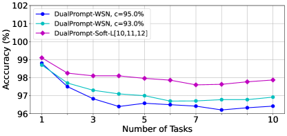
Sparsity of Transformer. We inspect the sparse solution through WSN as shown in Table 4, Table 10, and Table 11. We found a suboptimal sparse solution (c=87.0 % on 10-Split-TinyImageNet) with minimal CF through the inspections. This demonstrates the Rottary Ticket Hypothesis (RTH) in transformers, a competitive sparse subnetwork in DenseNetwork. In addition, DualPrompt is the lower-bound while DualPrompt-Soft-TF- is the upper-bound, close to the optimal performances.
 |
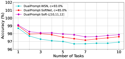 |
| (a) WSN-TransFormers v.s. Soft-TransFormers | (b) WSN v.s. SoftNet |
| TinyImageNet | ||||
| Method | Pretrained-Dataset | Task ID | ACC() | Forget() |
| DualPrompt | - | Prompt ID | 86.50 | 5.77 |
| DualPrompt-WSN-L[10,11,12] | C=80.0% | Gradient ID | 89.95 | 0.98 |
| DualPrompt-WSN-L[10,11,12] | C=81.0% | Gradient ID | 89.99 | 1.06 |
| DualPrompt-WSN-L[10,11,12] | C=82.0% | Gradient ID | 89.59 | 1.18 |
| DualPrompt-WSN-L[10,11,12] | C=83.0% | Gradient ID | 90.60 | 0.72 |
| DualPrompt-WSN-L[10,11,12] | C=85.0% | Gradient ID | 90.09 | 1.07 |
| DualPrompt-WSN-L[10,11,12] | C=87.0% | Gradient ID | 91.91 | 0.38 |
| DualPrompt-WSN-L[10,11,12] | C=90.0% | Gradient ID | 91.28 | 0.42 |
| DualPrompt-WSN-L[10,11,12] | C=93.0% | Gradient ID | 91.41 | 0.40 |
| DualPrompt-WSN-L[10,11,12] | C=95.0% | Gradient ID | 90.91 | 0.83 |
| DualPrompt-Soft-TF-L[10,11,12] | - | Gradient ID | 97.87 | 0.21 |
| Method | ViT-B/12 (85.8M) | 10-Split-CIFAR100 | 20-Split-CIFAR100 | 10-Split-ImageNet-R | ||||
| DualPrompt | # Train Params. | Task ID | ACC() | Forget() | ACC() | Forget() | ACC() | Forget() |
| DualPrompt | 0.00M | Prompt ID | 86.50 | 5.77 | 82.98 | 8.20 | 68.13 | 4.46 |
| PGP | 0.00M | Prompt ID | 86.92 | 5.35 | 83.74 | 7.91 | 69.34 | 4.53 |
| Soft-TF-L[12] w/ only ATTN | 1.76M | Gradient ID | 97.17 | 0.40 | 98.09 | 0.54 | 72.31 | 3.94 |
| Soft-TF-L[12] w/ only ATTN, WSN c=90% | 1.58M | Gradient ID | 96.81 | 0.61 | 97.51 | 1.68 | 71.67 | 3.94 |
Peudo Codes. The overall process of the Soft-TransFormers (Soft-TF) during training and testing is described as Algorithm 1 and Algorithm 2. We denote the architecture with attached prompts as . The input from the -th task is transformed using and then passed to the classification head , parameterized by , for prediction. Finally, we train the two prompts, the task keys, the soft-attention parameters, and the newly-initialized classification head in an end-to-end manner.
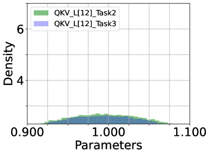
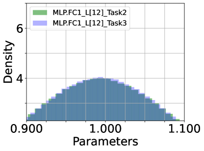
Density of Parameters. We inspect the histogram density estimate of the last (12) layer’s parameters of DualPrompt-Soft-TF: attention of QKV ((a) ATTN.QKV) and Projection ((b) ATTN.PROJ) and multi-layer perception (MLP) of FC1 and FC2, as shown in Figure 6. ATTN’s QKV parameters have the largest variance among the parameter densities, while MLP-FC2’s are the smallest. From this observation, we conclude that fine-tuning ATTN’s QKV is required to achieve optimal task performance. In other words, QKV’s parameters are more critical than others.
 |
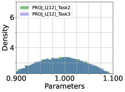 |
| (a) ATTN.QKV () | (b) ATTN.PROJ () |
 |
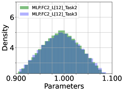 |
| (c) MLP.FC1 () | (d) MLP.FC2 () |
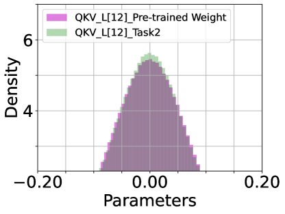
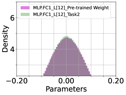
Pre-trained Parameters v.s. Soft-TF. We inspect the histogram density estimate of the last (12) layer’s parameters of pre-trained model and DualPrompt-Soft-TF: attention of QKV ((a) ATTN.QKV) and Projection ((b) ATTN.PROJ) and multi-layer perception (MLP) of FC1 and FC2, as shown in Figure 7. The most parameters of DualPrompt-Soft-TF are trained around zero-values. Particularly, the difference between pre-trained model’s parameters and Soft-TF is distinctive at QKV module.
 |
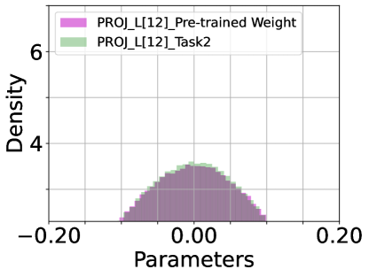 |
| (a) ATTN.QKV ( v.s. ) | (b) ATTN.PROJ ( v.s. ) |
 |
 |
| (c) MLP.FC1 ( v.s. ) | (d) MLP.FC2 ( v.s ) |
Public Source Code. All official source codes will be available soon.